Dynamics of Structures with Distributed Gyroscopes: Modal Discretization Versus Spatial Discretization

Abstract

In this study, two discretization numerical methods, modal discretization and spatial discretization methods, were proposed and compared when applied to the gyroscopic structures. If the distributed gyroscopes are attached, the general numerical methods should be modified to derive the natural frequencies and complex modes due to the gyroscopic effect. The modal discretization method can be used for cases where the modal functions of the base structure can be expressed in explicit forms, while the spatial discretization method can be used in irregular structures without modal functions, but cost more computational time. The convergence and efficiency of both modal and spatial discretization techniques are illustrated by an example of a beam with uniformly distributed gyroscopes. The investigation of this paper may provide useful techniques to study structures with distributed inertial components.

1. Introduction

Modern mechanical structures, especially intelligent flexible mechanical structures, are densely distributed with sensors, processors, and actuators [1]. Some transducers may apply inertial actions to the flexible structure, although they are also parts of the whole structure. In this study, structures with distributed gyroscopes will be studied, which has been verified as applicable in the control of soft structures such as space manipulation arms [2,3,4].

The gyroelastic continua have been proposed by Hughes and D’Eleuterio to describe the mathematical modeling of structures with continuously distributed gyroscopes [5,6]. The dynamics of flexible structures with distributed appendages can be investigated by modal discretization techniques such as the Galerkin method by introducing a set of trial mode functions, which are usually the modal functions of the corresponding structure without appendages [7,8,9]. Modal discretization techniques have shown powerful applications to structures with regular shapes (explicit modal functions) [10,11,12,13,14]. However, modal discretization becomes unpractical when treating structures with irregular or complicated contours. Without analytical modal functions, modal discretization loses the configuration base. Although the base modal shapes can be obtained by the finite element method and transferred to the modal discretization procedure, the manipulations are apparently cumbersome.

Spatial discretization techniques such as the finite element method could tackle the dynamics of structures with arbitrary shapes. However, the available commercial finite element software provides no general modules to treat flexible structures with distributed gyroscopes. The distributed gyroscopes introduce a new dynamic effect to the structures and the most important contribution is the gyroscopic coupling effect, which is usually neglected in low angular momentum examples. With increasing angular momentum, the gyroscopic coupling becomes dominating and varies the frequency and modal motion drastically [15,16,17,18,19,20]. Gyroscopic coupling can be employed as a mechanism of sensor to detect rotating angles, which has been discussed in the literature [21,22,23].

Although gyroscopic continua such as axially moving materials [24] and rotating components [25] have been studied widely, structures with discrete rotors have received less attention. In this study, we propose a spatial discretization technique designed to tackle flexible structures with distributed gyroscopes. The eigenfrequencies are studied and discussed. Both modal discretization and spatial discretization will be studied and compared by an example of gyroscope-distributed beam. The current study may expose the gyroscopic structures to more general numerical techniques.

2. Model Description

To validate the modal discretization and spatial discretization techniques, a beam model with uniformly distributed gyroscopes was studied and the natural frequencies and complex modes extracted and compared.

As described in Figure 1, an Euler beam supported by two hinges is distributed with N gyroscopes. The gyroscopes provide mass and angular momentum, but do not alter the deformation of the beam. The current simple model can be used directly to slender rotor systems [26,27], drill strings [28,29], and gyroscopic structures.

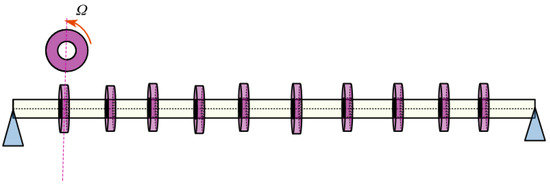
Figure 1. Diagram of an Euler beam with distributed gyroscopes.

3. Modal Discretization

To describe the displacements of the beam elements and gyroscope elements, two reference frames are used: the inertial frame F_b with the origin on one end of the beam on which the displacement of the beam is measured, and the non-inertial frame F_ri on which the rigid rotors are described (Figure 2). The undeformed position vector of an arbitrary small element dm in the beam is ${\overrightarrow{l}}_m$ measured in F_b, the displacement vector is ${\overrightarrow{u}}_m$, and the rotational angular vector is ${\overrightarrow{\beta }}_m$. Similarly, the undeformed position vector and the displacement vector of the element dm^ri on the ith rotor are ${\overrightarrow{l}}_{ri}$, ${\overrightarrow{u}}_{ri}$, and ${\overrightarrow{\beta }}_{ri}$, respectively. Measured on the non-inertial frame F_ri, the position vector of the rotor element is ${\overrightarrow{r}}_{ri}$. The rotating velocity of the rotor is ${\overrightarrow{\omega }}_{ri}={\Omega }_i={\left[{\Omega }_i,0,0\right]}^{\mathrm{T}}$ with respect to the frame F_ri.

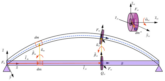
Figure 2. The displacements of the beam and the gyroscopes.

The translational and rotational displacements of the element dm can be cast into the generalized coordinates by using the beam’s modal functions without gyroscopes:

$${\overrightarrow{u}}_m=f_b^{\mathrm{T}}{T}_m{\mathsf{\tau }}_b$$

(1)

$${\overrightarrow{\beta }}_m=f_b^T{R}_m{\mathsf{\tau }}_b$$

(2)

where f_b is the matrix of unit vectors of the F_b basis vectors; T_m and R_m are the translational and rotational displacement vectors, respectively, the values of which are given by the sine functions of the supported beam modes on the element position; and τ_b is the generalized modal coordinate variable vector.

By the geometry of the elements shown in Figure 2, the total displacements of the beam and the ith rotor measured in F_b are

$${\overrightarrow{r}}_{m,b}={\overrightarrow{l}}_m+{\overrightarrow{u}}_m$$

(3)

$${\overrightarrow{r}}_{m,ri}={\overrightarrow{l}}_{ri}+{\overrightarrow{u}}_{ri}+{\overrightarrow{r}}_{ri}$$

(4)

The corresponding velocities are

$${\overrightarrow{v}}_{m,b}={\dot{\overrightarrow{u}}}_m$$

(5)

$${\overrightarrow{v}}_{m,ri}={\dot{\overrightarrow{u}}}_{ri}+{\dot{\overrightarrow{\beta }}}_{ri}\times {\overrightarrow{r}}_{ri}+{\overrightarrow{\omega }}_{ri}\times {\overrightarrow{r}}_{ri}$$

(6)

and the accelerations are

$${\overrightarrow{a}}_{m,b}={\ddot{\overrightarrow{u}}}_{m,b}$$

(7)

$${\overrightarrow{a}}_{m,ri}={\ddot{\overrightarrow{u}}}_{ri}+{\dot{\overrightarrow{\beta }}}_{ri}\times ({\dot{\overrightarrow{\beta }}}_{ri}\times {\overrightarrow{r}}_{m,ri})+{\dot{\overrightarrow{\beta }}}_{ri}\times ({\overrightarrow{\omega }}_{ri}\times {\overrightarrow{r}}_{m,ri})+{\ddot{\overrightarrow{\beta }}}_{ri}\times {\overrightarrow{r}}_{m,ri}+{\dot{\overrightarrow{\omega }}}_{ri}\times {\overrightarrow{r}}_{m,ri}$$

(8)

where ${\dot{\overrightarrow{\beta }}}_{ri}\times ({\dot{\overrightarrow{\beta }}}_{ri}\times {\overrightarrow{r}}_{m,ri})$ is small and ignored in Equation (8).

The velocities and accelerations can be expressed in the modal discretized variables by substituting Equations (1) and (2) into Equations (5)–(8):

$${\overrightarrow{v}}_{m,b}=f_b^T{T}_{m,b}{\dot{\mathsf{\tau }}}_b$$

(9)

$${\overrightarrow{v}}_{m,ri}=f_b^T(T_{ri}-A_{b,ri}{\tilde{r}}_{m,ri}{A}_{ri,b}{R}_{ri}){\dot{\mathsf{\tau }}}_b-f_{ri}^T{\tilde{r}}_{m,ri}{\Omega }_i$$

(10)

$${\overrightarrow{a}}_{m,b}=f_b^T{T}_{m,b}{\ddot{\mathsf{\tau }}}_b(1)$$

(11)

$${\overrightarrow{a}}_{m,ri}=f_b^T(T_{ri}-A_{b,ri}{\tilde{r}}_{m,ri}{A}_{ri,b}{R}_{ri}){\ddot{\mathsf{\tau }}}_b-f_{ri}^T{\dot{\tilde{\beta }}}_{ri}{\tilde{r}}_{m,ri}{\Omega }_i-f_{ri}^T{\tilde{r}}_{m,ri}{\dot{\Omega }}_i$$

(12)

where A_b,ri = f_bf_ri^T is the transform matrix between the two frames F_b and F_ri; f_b and f_ri are the unit vector of the F_b frame and F_ri frame, respectively; and ${\tilde{r}}_{m,ri}$ and ${\tilde{\beta }}_{ri}$ are the tilde matrix of vectors r_m,ri and β_ri, respectively.

To apply Kane’s Equation, the rotating velocity of each gyroscope should be considered as a generalized coordinate. Hence, the generalized coordinates and generalized velocities of the system are ${\left[{\mathsf{\tau }}_b{}^{\mathrm{T}},{\phi }_1,\dots ,{\phi }_i,\dots ,{\phi }_n\right]}^{\mathrm{T}}$ and ${\left[{\dot{\mathsf{\tau }}}_b{}^{\mathrm{T}},{\Omega }_1,\dots ,{\Omega }_i,\dots ,{\Omega }_n\right]}^{\mathrm{T}}$, respectively. If the first k order modes are used in the discretization, the number of generalized coordinates is k + n.

Based on Equation (9), the partial velocities of the beam element dm are

$${}^p\overrightarrow{v}{}_{m,b}^1=\frac{\partial {\overrightarrow{v}}_{m,b}}{\partial {\dot{\mathsf{\tau }}}_b}=f_b^T{T}_{m,b},$$

(13)

$${}^p\overrightarrow{v}{}_{m,b}^{1+i}=\frac{\partial {\overrightarrow{v}}_{m,b}}{\partial {\Omega }_i}=0(i=1,2,\dots ,n)$$

(14)

Based on Equation (10), the partial velocities of the ith gyroscopes are

$${}^p\overrightarrow{v}{}_{m,ri}^1=\frac{\partial {\overrightarrow{v}}_{m,ri}}{\partial {\dot{\mathsf{\tau }}}_b}=f_b^T(T_{ri}-A_{b,ri}{\tilde{r}}_{m,ri}{A}_{ri,b}{R}_{ri})$$

(15)

$${}^p\overrightarrow{v}{}_{m,ri}^{1+i}=\frac{\partial {\overrightarrow{v}}_{m,ri}}{\partial {\Omega }_i}=-f_{ri}^T{\tilde{r}}_{m,ri},(i=1,2,\dots ,n)$$

(16)

The generalized inertial forces of the beam and rotors can be obtained by integrating the product of the partial velocity and acceleration over all of the structure:

$$\begin{array}{ll}\hfill F^I& ={\displaystyle {\int }_{\mathrm{beam}}{}^p\overrightarrow{v}{}_b^1\cdot {\overrightarrow{a}}_{m,b}\mathrm{d}m}+{\displaystyle \sum _{i=1}^n{\displaystyle {\int }_{i\mathrm{th}\mathrm{rotor}}{}^p\overrightarrow{v}{}_{ri}^{1+i}\cdot {\overrightarrow{a}}_{m,ri}\mathrm{d}{m}^{ri}}}\hfill \\ & =E_a{\ddot{\mathsf{\tau }}}_b+{\displaystyle \sum (R_{ri}^T{A}_{b,ri}{\tilde{\dot{\beta }}}_{ri}{J}_{ri}^x{\Omega }_i)}+{\displaystyle \sum (R_{ri}^T{A}_{b,ri}{J}_{ri}^x{\dot{\Omega }}_i)},\hfill \end{array}$$

(17)

where

$$E_a=E_b+{\displaystyle \sum (m_{ri}^{}{T}_{ri}^T{T}_{ri}+R_{ri}^T{\widehat{J}}_{ri}^{}{R}_{ri})},E_b={{\displaystyle {\int }_{\mathrm{beam}}T}}_{m,b}^T{T}_{m,b}\mathrm{d}m$$

(18)

When the normalized modal functions are used, E_b is the identity matrix. Under the small deformation assumption, the transformation matrix A_{b, ri} and A_{ri, b} are approximately identity matrices, which makes the angular momentum vector of the gyroscopes

$${\widehat{J}}_{ri}=A_{b,ri}\cdot J_{ri}\cdot A_{ri,b}\approx J_{ri}=\mathrm{diag}(J_{ri}^x,J_{ri}^y,J_{ri}^z)$$

(19)

On the other hand, the generalized active force due to the nominal stiffness of the structure is

$$F^A={\Lambda }_b{\mathsf{\tau }}_b$$

(20)

where the stiffness matrix is defined as the diagonal array constituted by the square of the circular frequencies of the beam without any attachments,

$${\Lambda }_{\mathrm{b}}=diag({\omega }_1^2,\dots ,{\omega }_i^2,\dots ,{\omega }_m^2)$$

(21)

Substituting Equations (17) and (20) into Kane’s Equation

$$F_i^I+F_i^A=0$$

(22)

and neglecting the angular accelerations of the gyroscopes, one obtains the final ordinary differential equation governing the generalized displacement

$$E_a{\ddot{\mathsf{\tau }}}_b+G{\dot{\mathsf{\tau }}}_b+{\Lambda }_b{\mathsf{\tau }}_b=0$$

(23)

where the skew-symmetric gyroscopic matrix G is

$$G={\displaystyle \sum G_i},G_i=(R_{ri}^{2\mathrm{T}}{R}_{ri}^3-R_{ri}^{3\mathrm{T}}{R}_{ri}^2)J_{ri}^x{\Omega }_i$$

(24)

The superscript numbers in Equation (24) denote the row number of the corresponding matrix. The gyroscopic term expressed in the generalized coordinate in Equation (23) plays a key role, which leads to frequency bifurcation and complex modes.

The linear gyroscopic ordinary governing Equation (23) can be solved numerically and the natural frequencies and complex modes can be obtained by transferring the generalized variables back into physical deformations via relations (1) and (2).

4. Spatial Discretization

Spatial discretization is more adaptable than modal discretization when treating structures with complicated shapes, whose explicit mode functions cannot be obtained in a straightforward manner. In this study, we took the beam model with distributed gyroscopes to show the technique of spatial discretization. The segment of beam and segment of gyroscopes were considered as presented in Figure 3. This spatial discretization technique can also be expanded to other irregular structures.

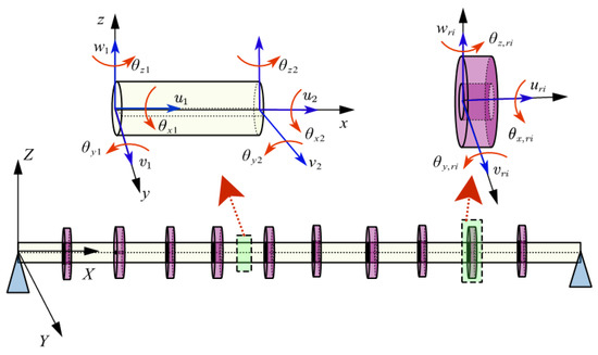
Figure 3. The diagrams of the beam element and gyroscope element.

Every node of the beam element has six DOFs, three translational displacements (u, v, w), and three rotational displacements (θ_x, θ_y, θ_z) along the three coordinates x, y, and z, respectively. The transversal rotational angles are

$${\theta }_y=\frac{\partial v}{\partial x},{\theta }_z=-\frac{\partial w}{\partial x}$$

(25)

The displacement vector of an arbitrary position in element e with length l_e is

$$\left\{{\Delta }^e(x)\right\}={\left[u,v,w,{\theta }_x,{\theta }_y,{\theta }_z\right]}^{\mathrm{T}}$$

(26)

The displacement vector can be expressed using the classical finite element cubic interpolating equation for bending deflections and linear interpolating equation for axial and torsional deflections, so that

$$\left\{{\Delta }^e(x)\right\}=\left[N\right]\left\{{\delta }^e\right\}$$

(27)

where [N] is the shape function matrix of the three-dimensional finite element, and the nodal displacement vector is

$$\left\{{\delta }^e\right\}={\left[u_1,v_1,w_1,{\theta }_{x1},{\theta }_{y1},{\theta }_{z1},u_2,v_2,w_2,{\theta }_{x2},{\theta }_{y2},{\theta }_{z2}\right]}^T$$

(28)

Equation (27) can be written as

$$\left\{\begin{array}{l}u(x)\\ v(x)\\ w(x)\end{array}\right\}=\left[N_T\right]\left\{{\delta }^e\right\},\left\{\begin{array}{l}{\theta }_y(x)\\ {\theta }_z(x)\end{array}\right\}=\left[N_{\theta }\right]\left\{{\delta }^e\right\}\left\{{\theta }_x(x)\right\}=\left[N_{\phi }\right]\left\{{\delta }^e\right\}$$

(29)

where [N_T], [N_θ], and [N_φ] are the translation, bending rotation, and torsional rotation shape function matrices, respectively. The shape function expressions can be found in the available references such as [28,30,31].

The element composed of a rigid gyroscope can be assumed as a distributed elastic beam with additional momentum. The ith gyroscope with finite length l_{e, ri} has the displacements

$$u_{ri}=u,v_{ri}=v,w_{ri}=w,{\theta }_{x,ri}={\theta }_x+\phi ,{\theta }_{y,ri}={\theta }_y,{\theta }_{z,ri}={\theta }_z$$

(30)

The gyroscope elements share the same features with beam elements except the extra gyroscope rotation angle φ. Hence, the kinetic energy an arbitrary element is

$$T=\frac{1}{2}{\displaystyle \underset{0}{\overset{l_{ej}}{\int }}(v_b{}^{\mathrm{T}}{m}_b{v}_b+{\omega }_b{}^{\mathrm{T}}{I}_b{\omega }_b)dx}+{\Delta }_{i,j}\frac{1}{2}{\displaystyle \underset{0}{\overset{l_{e,ri}}{\int }}(v_{ri}{}^{\mathrm{T}}{m}_{ri}{v}_{ri}+{\omega }_{ri}{}^{\mathrm{T}}{I}_{ri}{\omega }_{ri})dx}$$

(31)

where the symbol Δ_i,j denotes if the gyroscope i has been installed on the position j:

$${\Delta }_{i,j}=\{\begin{array}{l}1i=j,\\ 0i\ne j.\end{array}$$

(32)

The variables and parameters in Equation (31) are stated as follows. The mass density of the beam element and the ith gyroscope are m_b and m_ri, respectively. The translational and angular velocity vectors of the beam and gyroscopes are

$$v_b=\left[\begin{array}{l}\dot{u}\\ \dot{v}\\ \dot{w}\end{array}\right],{\omega }_b=\left[\begin{array}{c}{\dot{\theta }}_x-{\theta }_y{\dot{\theta }}_z\\ {\dot{\theta }}_y-{\dot{\theta }}_z{\theta }_x\\ {\dot{\theta }}_z+{\dot{\theta }}_y{\theta }_x\end{array}\right]$$

(33)

$$v_{ri}=\left[\begin{array}{l}\dot{u}\\ \dot{v}\\ \dot{w}\end{array}\right]{\omega }_{ri}=\left[\begin{array}{c}{\dot{\theta }}_x+\dot{\phi }-{\theta }_y\dot{\theta }{}_z\\ {\dot{\theta }}_y\cos ({\theta }_x+\phi )-\dot{\theta }{}_z\sin ({\theta }_x+\phi )\\ {\dot{\theta }}_z\cos ({\theta }_x+\phi )+\dot{\theta }{}_y\sin ({\theta }_x+\phi )\end{array}\right]$$

(34)

The moment of inertia of the beam element and the ith gyroscope are

$$I_b=\left[\begin{array}{ccc}{I}_p& 0& 0\\ 0& I_c& 0\\ 0& 0& I_c\end{array}\right],I_{ri}=\left[\begin{array}{ccc}{I}_{p,ri}& 0& 0\\ 0& I_{c,ri}& 0\\ 0& 0& I_{c,ri}\end{array}\right]$$

(35)

Substituting Equations (33)–(35) to Equation (31), the kinetic energy can simplified as

$$T=\frac{1}{2}{\left\{{\dot{\delta }}^e\right\}}^T\left[M^e\right]\left\{{\dot{\delta }}^e\right\}+{\Delta }_{i,j}\left(\frac{1}{2}{\left\{{\dot{\delta }}^e\right\}}^T\left[M^{e,ri}\right]\left\{{\dot{\delta }}^e\right\}-{\Omega }_i{\left\{{\dot{\delta }}^e\right\}}^T\left[G^{e,ri}\right]\left\{{\delta }^e\right\}\right)$$

(36)

where

$$\begin{array}{l}\left[M^e\right]=\left[M_T^e\right]+\left[M_{\phi }^e\right]+\left[M_{\theta }^e\right],\\ \left[M_T^e\right]={\displaystyle \underset{0}{\overset{l_e}{\int }}{m}_b{\left[N_T\right]}^{\mathrm{T}}\left[N_T\right]\mathrm{d}x},\left[M_{\phi }^e\right]={\displaystyle \underset{0}{\overset{l_e}{\int }}{I}_p{\left[N_{\phi }\right]}^{\mathrm{T}}\left[N_{\phi }\right]\mathrm{d}x},\left[M_{\theta }^e\right]={\displaystyle \underset{0}{\overset{l_e}{\int }}{I}_c{\left[N_{\theta }\right]}^{\mathrm{T}}\left[N_{\theta }\right]dx},\end{array}$$

(37)

$$\begin{array}{l}\left[M^{e,ri}\right]=\left[M_T^{e,ri}\right]+\left[M_{\theta }^{e,ri}\right]+\left[M_{\phi }^{e,ri}\right],\\ \left[M_T^{e,ri}\right]={\displaystyle \underset{0}{\overset{l_{e,ri}}{\int }}{m}_{ri}{\left[N_T\right]}^{\mathrm{T}}\left[N_T\right]\mathrm{d}x},\left[M_{\theta }^{e,ri}\right]={\displaystyle \underset{0}{\overset{l_{e,ri}}{\int }}{I}_{c,ri}{\left[N_{\theta }\right]}^{\mathrm{T}}\left[N_{\theta }\right]\mathrm{d}x,}\left[M_{\phi }^{e,ri}\right]={\displaystyle \underset{0}{\overset{l_{e,ri}}{\int }}{I}_{p,ri}{\left[N_{\phi }\right]}^{\mathrm{T}}\left[N_{\phi }\right]\mathrm{d}x},\end{array}$$

(38)

$$\left[G^{e,ri}\right]=\left[{\displaystyle \underset{0}{\overset{l_{e,ri}}{\int }}{I}_{p,ri}{\left[N_{{\theta }_z}\right]}^T\left[N_{{\theta }_y}\right]dx}\right]$$

(39)

The potential energy of the beam element is

$$U=\frac{1}{2}{\displaystyle \underset{0}{\overset{l_e}{\int }}EA{(\frac{\partial u}{\partial x})}^2\mathrm{d}x}+\frac{1}{2}{\displaystyle \underset{0}{\overset{l_e}{\int }}E{J}_y{(\frac{\partial {\theta }_y}{\partial x})}^2\mathrm{d}x+\frac{1}{2}{\displaystyle \underset{0}{\overset{l_e}{\int }}E{J}_z{(\frac{\partial {\theta }_z}{\partial x})}^2\mathrm{d}x}}+\frac{1}{2}{\displaystyle \underset{0}{\overset{l_e}{\int }}GJ{(\frac{\partial {\theta }_x}{\partial x})}^2\mathrm{d}x}$$

(40)

where A is the cross-sectional area; I_y and I_z are the area of moment of inertia around the y and z axes; and the J polar area moment of inertia. It is assumed that the gyroscopes do not contribute to the total potential energy.

Substituting the kinetic energy and potential energy into Lagrange Equation

$$\frac{\mathrm{d}}{\mathrm{d}t}(\frac{\partial L}{\partial \left\{{\dot{\delta }}^e\right\}})-\frac{\partial L}{\partial \left\{{\delta }^e\right\}}=\left\{Q^e\right\},L=U–T,$$

(41)

the governing equation of the jth element is then

$$\left[M_{ae}\right]\left\{{\ddot{\delta }}^e\right\}+{\Delta }_{i,j}{\Omega }_i\left[G_{ae}\right]\left\{{\dot{\delta }}^e\right\}+\left[K_{ae}\right]\left\{{\delta }^e\right\}=\left\{Q^e\right\}$$

(42)

where $\left\{Q^e\right\}$ is generalized active force, and

$$\left[M_{ae}\right]=\left[M^e\right]+{\Delta }_{i,j}\left[M^{e,ri}\right],\left[G_{ae}\right]={\left[G^{e,ri}\right]}^T-\left[G^{e,ri}\right],\left[K_{ae}\right]=\left[K^e\right].$$

(43)

When the gyroscopic term of Δ_i,j vanishes, the spatial discretized Equation (42) recovers to the classical one of a pure beam case.

By assembling the mass, gyroscopic and stiffness matrices of the individual elements, the global matrices of the entire structure can be obtained:

$$\left[M\right]\left\{\ddot{\delta }\right\}+{\Delta }_{i,j}{\Omega }_i\left[G\right]\left\{\dot{\delta }\right\}+\left[K\right]\left\{\delta \right\}=\left\{Q\right\}$$

(44)

where the N-nodes displacement vector is

$$\left\{\delta \right\}={\left[u_1,v_1,w_1,{\theta }_{x1},{\theta }_{y1},{\theta }_{z1},u_2,v_2,w_2,{\theta }_{x2},{\theta }_{y2},{\theta }_{z2},\dots \dots u_N,v_N,w_N,{\theta }_N,{\theta }_N,{\theta }_N\right]}^{\mathrm{T}}$$

(45)

Further applying the boundary conditions and neglecting the active forces, the final governing equations are

$$\left[M_o\right]\left\{{\ddot{\delta }}_o\right\}+{\Delta }_{i,j}{\Omega }_i\left[G_o\right]\left\{{\dot{\delta }}_o\right\}+\left[K_o\right]\left\{{\delta }_o\right\}=0$$

(46)

The Δ symbol describes the position where the gyroscopes are installed and the gyroscopic effect works in the vicinity of the exact position. While all of the gyroscopes are for the modal discretization case, Equation (23) takes the gyroscopic effect on the whole system.

5. Numerical Results and Comparison

To compare the modal discretization and spatial discretization techniques, a simply supported beam with ten uniformly distributed gyroscopes was studied as a demonstrating example. The length, density, cross section radius, Young’s modulus, and shear modulus were $10\mathrm{m}$, ${1200\mathrm{kg}/\mathrm{m}}^3$, $0.1\mathrm{m}$, ${7.84\times 10}^6\mathrm{Pa}$, ${2.667\times 10}^6\mathrm{Pa}$, respectively. The length, density, inner and outer radius for the each gyroscope were $0.082\mathrm{m}$, ${8000\mathrm{kg}/\mathrm{m}}^3$, 0.1 m, 0.2 m, respectively.

In Figure 4, the first four pairs of natural frequencies computed by 121 order modal discretization and 121-element spatial discretization are presented with varying angular momentum of the uniformly distributed gyroscopes. With the supplement of the gyroscopes, any one of the natural frequencies, denoting the planar modes, bifurcates into two, denoting the lower backward whirling (BW) and the higher forward whirling (FW) of three dimensional complex modes. The first four orders of the complex modes of both backward whirling and forward whirling are demonstrated in Figure 5. Similar phenomena on the frequency and complex mode appeared in [11], but the angular momentum was assumed to be continuously distributed.

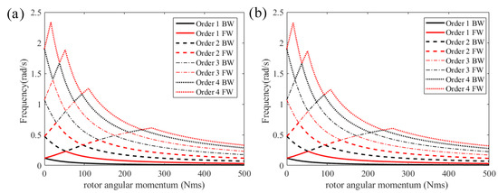
Figure 4. The varying natural frequencies with increasing angular momentum. (a) The results of the modal discretization. (b) The results of the spatial discretization.

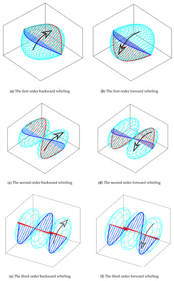
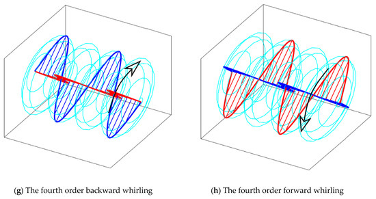
Figure 5. The vibration modes when $h=5\mathrm{Nms}$.

The varying frequencies with zig-zag configurations are related to the veering phenomenon, which has been discussed in gyroscopic structures such as rotors, blades, and gears [17,32,33,34]. In the current study, we did not consider the veering phenomenon, but focused on the numerical methods that have the power to show the gyroscopic dynamics.

To show the convergence of the two methods, the results from the different discretization orders are listed in Table 1, Table 2, Table 3, Table 4, Table 5, Table 6, Table 7, Table 8, Table 9, Table 10, Table 11, Table 12, Table 13, Table 14, Table 15, Table 16 and Table 17. The frequency unit in all tables is expressed as ‘rad/s’. In Table 1, Table 2, Table 3, Table 4, Table 5, Table 6, Table 7, Table 8 and Table 9, the natural frequencies for the different momentum of gyroscopes are presented to show the accuracy with the increasing modal discretization order k. It can be found that the results are satisfactory when the discretization order k is two times higher than the maximum mode being studied. If only lower vibration modes are used, the lower discretization order can be adopted to save computation time consumption. The modal discretization method has been shown to be efficient and powerful when dealing with a regular structure whose modal functions without attachments are explicit.

Table 1. Natural frequencies via modal discretization (h = 0).

	Order	1	2	3	4
K
11		0.119	0.476	1.071	1.904
33		0.119	0.476	1.071	1.904
55		0.119	0.476	1.071	1.903
77		0.119	0.476	1.071	1.903
99		0.119	0.476	1.071	1.903
121		0.119	0.476	1.071	1.903
165		0.119	0.476	1.071	1.903
187		0.119	0.476	1.071	1.903
209		0.119	0.476	1.071	1.903
231		0.119	0.476	1.071	1.903

Table 2. Natural frequencies via modal discretization (h = 100 Nms).

	Order	1 BW	1 FW	2 BW	2 FW	3 BW	3 FW	4 BW	4 FW
K
11		0.0377	0.150	0.340	0.360	0.618	1.005	1.404	3.246
33		0.0376	0.149	0.334	0.353	0.584	0.877	1.187	1.321
55		0.0375	0.147	0.324	0.344	0.558	0.844	1.170	1.223
77		0.0375	0.147	0.324	0.343	0.555	0.828	1.120	1.220
99		0.0374	0.146	0.322	0.341	0.550	0.822	1.116	1.202
121		0.0374	0.146	0.322	0.341	0.549	0.817	1.100	1.201
165		0.0374	0.146	0.321	0.341	0.547	0.812	1.092	1.195
187		0.0374	0.146	0.321	0.340	0.546	0.811	1.091	1.192
209		0.0374	0.146	0.320	0.340	0.546	0.810	1.089	1.192
231		0.0374	0.146	0.320	0.340	0.545	0.810	1.088	1.190

Table 3. Natural frequencies via modal discretization (h = 200 Nms).

	Order	1 BW	1 FW	2 BW	2 FW	3 BW	3 FW	4 BW	4 FW
K
11		0.0203	0.0805	0.185	0.338	0.574	0.632	2.265	4.801
33		0.0203	0.0799	0.181	0.314	0.468	0.576	0.623	0.784
55		0.0202	0.0786	0.174	0.297	0.449	0.536	0.615	0.781
77		0.0202	0.0785	0.174	0.295	0.437	0.534	0.584	0.726
99		0.0202	0.0782	0.173	0.292	0.435	0.526	0.582	0.725
121		0.0202	0.0782	0.173	0.291	0.431	0.526	0.573	0.710
165		0.0201	0.0781	0.172	0.290	0.429	0.523	0.568	0.703
187		0.0201	0.0781	0.172	0.289	0.428	0.522	0.568	0.703
209		0.0201	0.0781	0.172	0.289	0.427	0.521	0.566	0.700
231		0.0201	0.0780	0.172	0.289	0.427	0.521	0.566	0.699

Table 4. Natural frequencies via modal discretization (h = 300 Nms).

	Order	1 BW	1 FW	2 BW	2 FW	3 BW	3 FW	4 BW	4 FW
K
11		0.0138	0.0545	0.126	0.230	0.401	0.898	2.749	5.880
33		0.0137	0.0541	0.123	0.212	0.317	0.420	0.528	0.617
55		0.0137	0.0531	0.118	0.200	0.303	0.415	0.526	0.616
77		0.0137	0.0531	0.118	0.199	0.295	0.393	0.488	0.564
99		0.0136	0.0529	0.117	0.197	0.294	0.391	0.487	0.564
121		0.0136	0.0529	0.117	0.197	0.291	0.385	0.476	0.549
165		0.0136	0.0528	0.116	0.196	0.289	0.382	0.472	0.543
187		0.0136	0.0528	0.116	0.195	0.289	0.382	0.472	0.543
209		0.0136	0.0528	0.116	0.195	0.288	0.380	0.470	0.540
231		0.0136	0.0528	0.116	0.195	0.288	0.380	0.469	0.540

Table 5. Natural frequencies via modal discretization (h = 400 Nms).

	Order	1 BW	1 FW	2 BW	2 FW	3 BW	3 FW	4 BW	4 FW
K
11		0.0104	0.0411	0.0950	0.174	0.308	1.157	2.991	7.246
33		0.0104	0.0408	0.0927	0.160	0.239	0.316	0.397	0.464
55		0.0103	0.0401	0.0891	0.151	0.229	0.312	0.396	0.463
77		0.0103	0.0401	0.0890	0.150	0.223	0.295	0.367	0.424
99		0.0103	0.0399	0.0882	0.148	0.221	0.295	0.367	0.423
121		0.0103	0.0399	0.0882	0.148	0.219	0.290	0.358	0.412
165		0.0103	0.0398	0.0879	0.147	0.218	0.287	0.355	0.408
187		0.0103	0.0398	0.0877	0.147	0.218	0.287	0.355	0.408
209		0.0103	0.0398	0.0877	0.147	0.217	0.286	0.353	0.405
231		0.0103	0.0398	0.0877	0.147	0.217	0.286	0.353	0.405

Table 6. Natural frequencies via modal discretization (h = 500 Nms).

	Order	1 BW	1 FW	2 BW	2 FW	3 BW	3 FW	4 BW	4 FW
K
11		0.00832	0.0330	0.0763	0.140	0.249	1.404	3.144	8.741
33		0.00830	0.0327	0.0744	0.129	0.192	0.253	0.318	0.371
55		0.00827	0.0321	0.0715	0.121	0.184	0.250	0.317	0.370
77		0.00827	0.0321	0.0714	0.120	0.179	0.237	0.294	0.339
99		0.00826	0.0320	0.0708	0.119	0.177	0.236	0.294	0.339
121		0.00826	0.0320	0.0707	0.119	0.176	0.232	0.287	0.330
165		0.00825	0.0319	0.0705	0.118	0.175	0.230	0.284	0.326
187		0.00825	0.0319	0.0704	0.118	0.174	0.230	0.284	0.326
209		0.00825	0.0319	0.0704	0.118	0.174	0.229	0.283	0.324
231		0.00825	0.0319	0.0703	0.118	0.174	0.229	0.283	0.324

Table 7. Natural frequencies via modal discretization (h = 1000 Nms).

	Order	1 BW	1 FW	2 BW	2 FW	3 BW	3 FW	4 BW	4 FW
K
11		0.00418	0.0166	0.0383	0.0703	0.127	2.263	3.984	16.713
33		0.00417	0.0164	0.0374	0.0645	0.0962	0.127	0.159	0.186
55		0.00415	0.0161	0.0359	0.0607	0.0922	0.125	0.159	0.185
77		0.00415	0.0161	0.0358	0.0604	0.0896	0.119	0.147	0.170
99		0.00414	0.0160	0.0355	0.0597	0.0890	0.118	0.147	0.170
121		0.00414	0.0160	0.0355	0.0596	0.0883	0.116	0.144	0.165
143		0.00414	0.0160	0.0354	0.0593	0.0880	0.116	0.144	0.165
165		0.00414	0.0160	0.0354	0.0592	0.0877	0.115	0.142	0.163
187		0.00414	0.0160	0.0353	0.0591	0.0875	0.115	0.142	0.163
209		0.00414	0.0160	0.0353	0.0591	0.0874	0.115	0.142	0.162
231		0.00414	0.0160	0.0353	0.0590	0.0873	0.115	0.142	0.162

Table 8. Natural frequencies via modal discretization (h = 2000 Nms).

	Order	1 BW	1 FW	2 BW	2 FW	3 BW	3 FW	4 BW	4 FW
K
11		0.00209	0.00828	0.0192	0.0352	0.0638	2.618	6.913	33.071
33		0.00209	0.00821	0.0187	0.0323	0.0482	0.0635	0.0798	0.0929
55		0.00208	0.00806	0.0180	0.0304	0.0461	0.0627	0.0796	0.0928
77		0.00208	0.00806	0.0179	0.0302	0.0449	0.0593	0.0737	0.0849
99		0.00207	0.00803	0.0178	0.0299	0.0446	0.0591	0.0736	0.0848
121		0.00207	0.00803	0.0178	0.0298	0.0442	0.0581	0.0719	0.0826
165		0.00207	0.00801	0.0177	0.0296	0.0439	0.0577	0.0712	0.0816
187		0.00207	0.00801	0.0177	0.0296	0.0438	0.0576	0.0712	0.0816
209		0.00207	0.00801	0.0177	0.0296	0.0437	0.0574	0.0709	0.0812
231		0.00207	0.00801	0.0177	0.0295	0.0437	0.0574	0.0709	0.0812

Table 9. Natural frequencies via spatial discretization (h = 0).

	Order	1	2	3	4
Element Number
22		0.117	0.469	1.061	1.897
33		0.118	0.472	1.064	1.895
44		0.118	0.474	1.066	1.897
66		0.119	0.475	1.069	1.899
88		0.119	0.476	1.070	1.900
99		0.118	0.473	1.063	1.886
110		0.119	0.475	1.067	1.894
121		0.119	0.476	1.071	1.901
242		0.119	0.477	1.072	1.903
484		0.119	0.477	1.072	1.903

Table 10. Natural frequencies via spatial discretization (h = 100 Nms).

	Order	1 BW	1 FW	2 BW	2 FW	3 BW	3 FW	4 BW	4 FW
Element Number
22		0.0392	0.150	0.293	0.330	0.556	0.822	1.097	1.127
33		0.0383	0.148	0.317	0.326	0.552	0.820	1.102	1.138
44		0.0380	0.147	0.324	0.327	0.550	0.816	1.096	1.153
66		0.0377	0.146	0.322	0.335	0.547	0.812	1.091	1.170
88		0.0376	0.146	0.321	0.338	0.546	0.810	1.088	1.179
99		0.0354	0.130	0.291	0.347	0.472	0.712	1.032	1.204
110		0.0365	0.139	0.308	0.344	0.507	0.769	1.062	1.206
121		0.0370	0.144	0.316	0.344	0.538	0.797	1.070	1.194
242		0.0373	0.145	0.319	0.344	0.544	0.806	1.082	1.195
484		0.0373	0.145	0.319	0.345	0.543	0.805	1.081	1.199

Table 11. Natural frequencies via spatial discretization (h = 200 Nms).

	Order	1 BW	1 FW	2 BW	2 FW	3 BW	3 FW	4 BW	4 FW
Element Number
22		0.0213	0.0810	0.180	0.299	0.423	0.444	0.584	0.728
33		0.0207	0.0795	0.176	0.294	0.436	0.471	0.576	0.715
44		0.0205	0.0789	0.174	0.292	0.432	0.491	0.572	0.708
66		0.0203	0.0784	0.173	0.290	0.429	0.509	0.567	0.701
88		0.0202	0.0782	0.172	0.289	0.427	0.517	0.565	0.699
99		0.0189	0.0688	0.155	0.249	0.372	0.527	0.536	0.624
110		0.0196	0.0739	0.165	0.267	0.403	0.525	0.551	0.656
121		0.0199	0.0768	0.169	0.284	0.420	0.527	0.555	0.686
242		0.0201	0.0778	0.171	0.288	0.424	0.529	0.562	0.694
484		0.0201	0.0777	0.171	0.287	0.424	0.533	0.561	0.692

Table 12. Natural frequencies via spatial discretization (h = 300 Nms).

	Order	1 BW	1 FW	2 BW	2 FW	3 BW	3 FW	4 BW	4 FW
Element Number
22		0.0145	0.0548	0.123	0.202	0.303	0.396	0.495	0.506
33		0.0140	0.0538	0.119	0.199	0.295	0.388	0.481	0.553
44		0.0139	0.0534	0.118	0.197	0.292	0.384	0.476	0.547
66		0.0138	0.0530	0.117	0.196	0.290	0.381	0.471	0.541
88		0.0137	0.0529	0.117	0.195	0.288	0.380	0.469	0.539
99		0.0128	0.0464	0.105	0.168	0.250	0.360	0.420	0.498
110		0.0133	0.0499	0.112	0.180	0.272	0.370	0.440	0.517
121		0.0134	0.0519	0.114	0.192	0.283	0.373	0.460	0.529
242		0.0136	0.0526	0.116	0.194	0.286	0.377	0.465	0.535
484		0.0136	0.0525	0.115	0.194	0.286	0.377	0.464	0.534

Table 13. Natural frequencies via spatial discretization (h = 400 Nms).

	Order	1 BW	1 FW	2 BW	2 FW	3 BW	3 FW	4 BW	4 FW
Element Number
22		0.0109	0.0414	0.0927	0.153	0.229	0.299	0.374	0.429
33		0.0106	0.0406	0.0901	0.150	0.223	0.292	0.362	0.416
44		0.0105	0.0402	0.0891	0.148	0.220	0.289	0.358	0.411
66		0.0104	0.0400	0.0883	0.147	0.218	0.287	0.354	0.406
88		0.0103	0.0399	0.0879	0.147	0.217	0.286	0.353	0.405
99		0.0096	0.0349	0.0793	0.126	0.189	0.271	0.316	0.374
110		0.0100	0.0376	0.0842	0.136	0.205	0.278	0.331	0.388
121		0.0101	0.0391	0.0863	0.144	0.213	0.281	0.346	0.397
242		0.0103	0.0396	0.0873	0.146	0.216	0.284	0.350	0.401
484		0.0102	0.0396	0.0871	0.146	0.215	0.283	0.349	0.401

Table 14. Natural frequencies via spatial discretization (h = 500 Nms).

	Order	1 BW	1 FW	2 BW	2 FW	3 BW	3 FW	4 BW	4 FW
Element Number
22		0.00876	0.0332	0.0745	0.1226	0.184	0.240	0.300	0.344
33		0.00850	0.0325	0.0723	0.1201	0.179	0.234	0.291	0.333
44		0.00841	0.0323	0.0715	0.1191	0.177	0.232	0.287	0.329
66		0.00832	0.0321	0.0708	0.1182	0.175	0.230	0.284	0.325
88		0.00829	0.0320	0.0705	0.1178	0.174	0.229	0.282	0.324
99		0.00772	0.0280	0.0636	0.1011	0.151	0.217	0.253	0.300
110		0.00802	0.0301	0.0675	0.1088	0.164	0.223	0.265	0.311
121		0.00813	0.0314	0.0692	0.1157	0.171	0.225	0.277	0.318
242		0.00823	0.0318	0.0700	0.1171	0.173	0.227	0.280	0.321
484		0.00821	0.0317	0.0699	0.1169	0.173	0.227	0.280	0.321

Table 15. Natural frequencies via spatial discretization (h = 1000 Nms).

	Order	1 BW	1 FW	2 BW	2 FW	3 BW	3 FW	4 BW	4 FW
Element Number
22		0.00440	0.0167	0.0375	0.0616	0.0928	0.120	0.151	0.172
33		0.00427	0.0163	0.0363	0.0602	0.0898	0.117	0.146	0.167
44		0.00422	0.0162	0.0359	0.0597	0.0887	0.116	0.144	0.164
66		0.00418	0.0161	0.0356	0.0593	0.0878	0.115	0.142	0.163
88		0.00416	0.0160	0.0354	0.0590	0.0874	0.115	0.142	0.162
99		0.00387	0.0140	0.0319	0.0507	0.0758	0.109	0.127	0.150
110		0.00402	0.0151	0.0339	0.0545	0.0824	0.112	0.133	0.155
121		0.00408	0.0157	0.0347	0.0580	0.0858	0.113	0.139	0.159
242		0.00413	0.0159	0.0351	0.0587	0.0868	0.114	0.140	0.161
484		0.00412	0.0159	0.0351	0.0586	0.0866	0.114	0.140	0.160

Table 16. Natural frequencies via spatial discretization (h = 2000 Nms).

	Order	1 BW	1 FW	2 BW	2 FW	3 BW	3 FW	4 BW	4 FW
Element Number
22		0.00220	0.00834	0.0188	0.0308	0.0465	0.0602	0.0756	0.0862
33		0.00214	0.00817	0.0182	0.0301	0.0450	0.0587	0.0729	0.0833
44		0.00211	0.00810	0.0180	0.0299	0.0444	0.0581	0.0719	0.0823
66		0.00209	0.00805	0.0178	0.0296	0.0440	0.0576	0.0711	0.0814
88		0.00208	0.00802	0.0177	0.0295	0.0438	0.0573	0.0708	0.0810
99		0.00194	0.00702	0.0160	0.0254	0.0379	0.0544	0.0634	0.0750
110		0.00201	0.00756	0.0170	0.0273	0.0412	0.0558	0.0665	0.0777
121		0.00204	0.00788	0.0174	0.0290	0.0429	0.0563	0.0695	0.0795
242		0.00207	0.00798	0.0176	0.0294	0.0434	0.0570	0.0702	0.0804
484		0.00206	0.00797	0.0175	0.0293	0.0433	0.0569	0.0701	0.0802

Table 17. Comparison between modal and spatial discretization.

Order		1 BW	1 FW	2 BW	2 FW	3 BW	3 FW	4 BW	4 FW
100 Nms	Modal	0.0374	0.146	0.322	0.341	0.549	0.817	1.100	1.201
	Spatial	0.0370	0.144	0.316	0.344	0.538	0.797	1.070	1.194
	Deviation (%)	1.27	1.51	1.77	−0.82	2.15	2.41	2.70	0.58
200 Nms	Modal	0.0202	0.0782	0.173	0.291	0.431	0.526	0.573	0.710
	Spatial	0.0199	0.0768	0.169	0.284	0.420	0.527	0.555	0.686
	Deviation (%)	1.45	1.77	2.03	2.48	2.70	−0.23	3.01	3.33
300 Nms	Modal	0.0136	0.0529	0.117	0.197	0.291	0.385	0.476	0.549
	Spatial	0.0134	0.0519	0.114	0.192	0.283	0.373	0.460	0.529
	Deviation (%)	1.49	1.83	2.10	2.57	2.77	3.09	3.39	3.68
400 Nms	Modal	0.0103	0.0399	0.0882	0.148	0.219	0.290	0.358	0.412
	Spatial	0.0101	0.0391	0.0863	0.144	0.213	0.281	0.346	0.397
	Deviation (%)	1.51	1.85	2.13	2.61	2.80	3.12	3.41	3.70
500 Nms	Modal	0.00826	0.0320	0.0707	0.119	0.176	0.232	0.287	0.330
	Spatial	0.00813	0.0314	0.0692	0.116	0.171	0.225	0.277	0.318
	Deviation (%)	1.52	1.86	2.14	2.62	2.81	3.14	3.42	3.70
600 Nms	Modal	0.00689	0.0267	0.0590	0.0991	0.147	0.193	0.239	0.275
	Spatial	0.00679	0.0262	0.0578	0.0965	0.143	0.187	0.231	0.265
	Deviation (%)	1.52	1.86	2.15	2.63	2.83	3.15	3.43	3.71
1000 Nms	Modal	0.00414	0.0160	0.0355	0.0596	0.0883	0.116	0.144	0.165
	Spatial	0.00408	0.0157	0.0347	0.0580	0.0858	0.113	0.139	0.159
	Deviation (%)	1.53	1.88	2.16	2.64	2.83	3.16	3.44	3.72
1500 Nms	Modal	0.00276	0.0107	0.0237	0.0397	0.0589	0.0775	0.0959	0.110
	Spatial	0.00272	0.0105	0.0232	0.0387	0.0572	0.0750	0.0926	0.106
	Deviation (%)	1.53	1.88	2.16	2.65	2.84	3.16	3.44	3.72
2000 Nms	Modal	0.00207	0.00803	0.0178	0.0298	0.0442	0.0581	0.0719	0.0826
	Spatial	0.00204	0.00788	0.0174	0.0290	0.0429	0.0563	0.0695	0.0795
	Deviation (%)	1.53	1.88	2.17	2.65	2.84	3.17	3.44	3.72

The spatial discretization method provides an efficient technique to treat irregular structures. In Table 9, Table 10, Table 11, Table 12, Table 13, Table 14, Table 15 and Table 16, the natural frequencies are listed for different angular momentum to show the convergence with increasing element numbers. The power of the spatial discretization has been demonstrated by satisfactory results. With increasing element numbers, the computation time will increase. However, lower order discretization may provide data with sufficient accuracy. Compared to modal discretization, more computational cost is required. Such a drawback opens the chance to deal with structures of irregular shapes.

For both methods, the higher gyroscope momentum requires higher order discretization to ensure accuracy. In Table 17, the results of the modal discretization and spatial discretization were compared with the gyroscope momentum up to 2000 Nms, where the 240 order discretization was used. The deviations between the natural frequencies of the two methods were less than 5%, which validates the accuracy of both methods.

6. Conclusions

In this paper, modal discretization and spatial discretization methods were presented and compared in the study of a flexible structure with distributed gyroscopes. Using the gyroscopic beam example, it was found that the modal discretization was more efficient when dealing with lower order vibration modes and the spatial discretization costs more computation time. The modal discretization method requires explicit mode functions of the base structure, which is not applicable to irregular components. The spatial discretization method allows manipulations of flexible structures of any shape, although the computation cost is higher.

References

- Brocato, M.; Capriz, G. Control of Beams and Chains through Distributed Gyroscopes. AIAA J. 2009, 47, 294–302. [Google Scholar] [CrossRef]
- Damaren, C.J.; Deleuterio, G.M.T. Optimal-Control of Large Space Structures Using Distributed Gyricity. J. Guid. Control Dynam. 1989, 12, 723–731. [Google Scholar] [CrossRef]
- Damaren, C.J.; Deleuterio, G.M.T. Controllability and Observability of Gyroelastic Vehicles. J. Guid. Control Dynam. 1991, 14, 886–894. [Google Scholar] [CrossRef]
- Yamanaka, K.; Heppler, G.R.; Huseyin, K. Stability of gyroelastic beams. AIAA J. 1996, 34, 1270–1278. [Google Scholar] [CrossRef]
- Deleuterio, G.M.T.; Hughes, P.C. Dynamics of Gyroelastic Continua. J. Appl. Mech. 1984, 51, 415–422. [Google Scholar] [CrossRef]
- Hughes, P.C.; D’Eleuterio, G.M. Modal parameter analysis of gyroelastic continua. J. Appl. Mech. 1986, 53, 919–924. [Google Scholar] [CrossRef]
- Hu, Q.; Jia, Y.; Xu, S. Dynamics and vibration suppression of space structures with control moment gyroscopes. Acta Astronaut. 2014, 96, 232–245. [Google Scholar] [CrossRef]
- Hu, Q.; Jia, Y.; Hu, H.; Xu, S.; Zhang, J. Dynamics and Modal Analysis of Gyroelastic Body with Variable Speed Control Moment Gyroscopes. J. Comput. Nonlin. Dyn. 2016, 11, 044506. [Google Scholar] [CrossRef]
- Hu, Q.; Guo, C.D.; Zhang, J. Singularity and steering logic for control moment gyros on flexible space structures. Acta Astronaut. 2017, 137, 261–273. [Google Scholar] [CrossRef]
- Ding, H.; Lu, Z.Q.; Chen, L.Q. Nonlinear isolation of transverse vibration of pre-pressure beams. J. Sound Vib. 2019, 442, 738–751. [Google Scholar] [CrossRef]
- Hassanpour, S.; Heppler, G.R. Dynamics of 3D Timoshenko gyroelastic beams with large attitude changes for the gyros. Acta Astronaut. 2016, 118, 33–48. [Google Scholar] [CrossRef]
- Brake, M.R.; Wickert, J.A. Modal analysis of a continuous gyroscopic second-order system with nonlinear constraints. J. Sound Vib. 2010, 329, 893–911. [Google Scholar] [CrossRef]
- Ding, H.; Ji, J.C.; Chen, L.Q. Nonlinear vibration isolation for fluid-conveying pipes using quasi-zero stiffness characteristics. Mech. Syst. Signal Process. 2019, 121, 675–688. [Google Scholar] [CrossRef]
- Ding, H.; Wang, S.; Zhang, Y.W. Free and forced nonlinear vibration of a transporting belt with pulley support ends. Nonlinear Dyn. 2018, 92, 2037–2048. [Google Scholar] [CrossRef]
- Yang, X.-D.; Yang, J.-H.; Qian, Y.-J.; Zhang, W.; Melnik, R.V.N. Dynamics of a beam with both axial moving and spinning motion: An example of bi-gyroscopic continua. Eur. J. Mech. A/Solids 2018, 69, 231–237. [Google Scholar] [CrossRef]
- Carta, G.; Jones, I.S.; Movchan, N.V.; Movchan, A.B.; Nieves, M.J. Gyro-elastic beams for the vibration reduction of long flexural systems. Proc. R. Soc. A: Math. Phys. Eng. Sci. 2017, 473. [Google Scholar] [CrossRef]
- Cooley, C.G.; Parker, R.G. Eigenvalue sensitivity and veering in gyroscopic systems with application to high-speed planetary gears. Eur. J. Mech. A Solids 2018, 67, 123–136. [Google Scholar] [CrossRef]
- Addari, D.; Aglietti, G.S.; Remedia, M. Dynamic Mass of a Reaction Wheel Including Gyroscopic Effects: An Experimental Approach. AIAA J. 2017, 55, 274–285. [Google Scholar] [CrossRef]
- Shabana, A.A. On the definition of the natural frequency of oscillations in nonlinear large rotation problems. J. Sound Vib. 2010, 329, 3171–3181. [Google Scholar] [CrossRef]
- Liu, T.; Zhang, W.; Mao, J.J.; Zheng, Y. Nonlinear breathing vibrations of eccentric rotating composite laminated circular cylindrical shell subjected to temperature, rotating speed and external excitations. Mech. Syst. Signal Process. 2019, 127, 463–498. [Google Scholar] [CrossRef]
- Acar, C.; Shkel, A. MEMS Vibratory Gyroscopes: Structural Approaches to Improve Robustness; Springer: Boston, MA, USA, 2009. [Google Scholar] [CrossRef]
- Dell’Olio, F.; Ciminelli, C.; Armenise, M.N. Theoretical investigation of indium phosphide buried ring resonators for new angular velocity sensors. Opt. Eng. 2013, 52, p024601. [Google Scholar] [CrossRef]
- Dell’Olio, F.; Tatoli, T.; Ciminelli, C.; Armenise, M.N. Recent advances in miniaturized optical gyroscopes. J. Eur. Opt. Soc. Rapid Publ. 2014, 9. [Google Scholar] [CrossRef]
- Luo, Z.; Hutton, S.G. Formulation of a three-node traveling triangular plate element subjected to gyroscopic and in-plane forces. Comput. Struct. 2002, 80, 1935–1944. [Google Scholar] [CrossRef]
- Özşahin, O.; Özgüven, H.N.; Budak, E. Analytical modeling of asymmetric multi-segment rotor—Bearing systems with Timoshenko beam model including gyroscopic moments. Comput. Struct. 2014, 144, 119–126. [Google Scholar] [CrossRef]
- Mohiuddin, M.A.; Khulief, Y.A. Modal Characteristics of Rotors Using a Conical Shaft Finite-Element. Comput. Methods Appl. Mech. Eng. 1994, 115, 125–144. [Google Scholar] [CrossRef]
- Mohiuddin, M.A.; Khulief, Y.A. Modal characteristics of cracked rotors using a conical shaft finite element. Comput. Methods Appl. Mech. Eng. 1998, 162, 223–247. [Google Scholar] [CrossRef]
- Alsaffar, Y.; Sassi, S.; Baz, A. Band Gap Characteristics of Nonrotating Passive Periodic Drill String. J. Vib. Acoust. 2018, 140. [Google Scholar] [CrossRef]
- Alsaffar, Y.; Sassi, S.; Baz, A. Band gap characteristics of periodic gyroscopic systems. J. Sound Vib. 2018, 435, 301–322. [Google Scholar] [CrossRef]
- Nelson, H.D. A Finite Rotating Shaft Element Using Timoshenko Beam Theory. J. Mech. Des. 1980, 102, 793–803. [Google Scholar] [CrossRef]
- Bazoune, A.; Khulief, Y.A.; Stephen, N.G. Shape functions of three-dimensional Timoshenko beam element. J. Sound Vib. 2003, 259, 473–480. [Google Scholar] [CrossRef]
- Lin, J.; Parker, R.G. Natural frequency veering in planetary gears. Mech. Struct. Mach. 2001, 29, 411–429. [Google Scholar] [CrossRef]
- Vidoli, S.; Vestroni, F. Veering phenomena in systems with gyroscopic coupling. J. Appl. Mech. 2005, 72, 641–647. [Google Scholar] [CrossRef]
- Shi, C.Z.; Parker, R.G. Vibration Modes and Natural Frequency Veering in Three-Dimensional, Cyclically Symmetric Centrifugal Pendulum Vibration Absorber Systems. J. Vib. Acoust. 2014, 136, 011014. [Google Scholar] [CrossRef]
© 2019 by the authors. Licensee MDPI, Basel, Switzerland. This article is an open access article distributed under the terms and conditions of the Creative Commons Attribution (CC BY) license (http://creativecommons.org/licenses/by/4.0/).