Article

Dynamics of Structures with Distributed Gyroscopes: Modal Discretization Versus Spatial Discretization

1
Beijing Key Laboratory of Nonlinear Vibrations and Strength of Mechanical Structures College of Mechanical Engineering, Beijing University of Technology, Beijing 100124, China
2
School of Aerospace Engineering, Beijing Institute of Technology, Beijing 100081, China
*
Author to whom correspondence should be addressed.
Appl. Sci. 2020, 10(1), 160; https://doi.org/10.3390/app10010160
Submission received: 6 November 2019 / Revised: 17 December 2019 / Accepted: 19 December 2019 / Published: 24 December 2019
(This article belongs to the Section Acoustics and Vibrations)

Abstract

:
In this study, two discretization numerical methods, modal discretization and spatial discretization methods, were proposed and compared when applied to the gyroscopic structures. If the distributed gyroscopes are attached, the general numerical methods should be modified to derive the natural frequencies and complex modes due to the gyroscopic effect. The modal discretization method can be used for cases where the modal functions of the base structure can be expressed in explicit forms, while the spatial discretization method can be used in irregular structures without modal functions, but cost more computational time. The convergence and efficiency of both modal and spatial discretization techniques are illustrated by an example of a beam with uniformly distributed gyroscopes. The investigation of this paper may provide useful techniques to study structures with distributed inertial components.

1. Introduction

Modern mechanical structures, especially intelligent flexible mechanical structures, are densely distributed with sensors, processors, and actuators [1]. Some transducers may apply inertial actions to the flexible structure, although they are also parts of the whole structure. In this study, structures with distributed gyroscopes will be studied, which has been verified as applicable in the control of soft structures such as space manipulation arms [2,3,4].
The gyroelastic continua have been proposed by Hughes and D’Eleuterio to describe the mathematical modeling of structures with continuously distributed gyroscopes [5,6]. The dynamics of flexible structures with distributed appendages can be investigated by modal discretization techniques such as the Galerkin method by introducing a set of trial mode functions, which are usually the modal functions of the corresponding structure without appendages [7,8,9]. Modal discretization techniques have shown powerful applications to structures with regular shapes (explicit modal functions) [10,11,12,13,14]. However, modal discretization becomes unpractical when treating structures with irregular or complicated contours. Without analytical modal functions, modal discretization loses the configuration base. Although the base modal shapes can be obtained by the finite element method and transferred to the modal discretization procedure, the manipulations are apparently cumbersome.
Spatial discretization techniques such as the finite element method could tackle the dynamics of structures with arbitrary shapes. However, the available commercial finite element software provides no general modules to treat flexible structures with distributed gyroscopes. The distributed gyroscopes introduce a new dynamic effect to the structures and the most important contribution is the gyroscopic coupling effect, which is usually neglected in low angular momentum examples. With increasing angular momentum, the gyroscopic coupling becomes dominating and varies the frequency and modal motion drastically [15,16,17,18,19,20]. Gyroscopic coupling can be employed as a mechanism of sensor to detect rotating angles, which has been discussed in the literature [21,22,23].
Although gyroscopic continua such as axially moving materials [24] and rotating components [25] have been studied widely, structures with discrete rotors have received less attention. In this study, we propose a spatial discretization technique designed to tackle flexible structures with distributed gyroscopes. The eigenfrequencies are studied and discussed. Both modal discretization and spatial discretization will be studied and compared by an example of gyroscope-distributed beam. The current study may expose the gyroscopic structures to more general numerical techniques.

2. Model Description

To validate the modal discretization and spatial discretization techniques, a beam model with uniformly distributed gyroscopes was studied and the natural frequencies and complex modes extracted and compared.
As described in Figure 1, an Euler beam supported by two hinges is distributed with N gyroscopes. The gyroscopes provide mass and angular momentum, but do not alter the deformation of the beam. The current simple model can be used directly to slender rotor systems [26,27], drill strings [28,29], and gyroscopic structures.

3. Modal Discretization

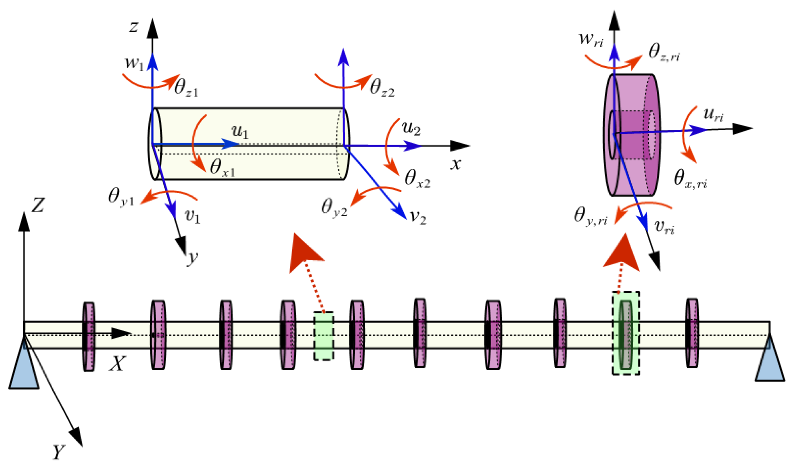
To describe the displacements of the beam elements and gyroscope elements, two reference frames are used: the inertial frame Fb with the origin on one end of the beam on which the displacement of the beam is measured, and the non-inertial frame Fri on which the rigid rotors are described (Figure 2). The undeformed position vector of an arbitrary small element dm in the beam is l m measured in Fb, the displacement vector is u m , and the rotational angular vector is β m . Similarly, the undeformed position vector and the displacement vector of the element dmri on the ith rotor are l r i , u r i , and β r i , respectively. Measured on the non-inertial frame Fri, the position vector of the rotor element is r r i . The rotating velocity of the rotor is ω r i = Ω i = [ Ω i , 0 , 0 ] T with respect to the frame Fri.
The translational and rotational displacements of the element dm can be cast into the generalized coordinates by using the beam’s modal functions without gyroscopes:
u m = f b T T m τ b
β m = f b T R m τ b
where fb is the matrix of unit vectors of the Fb basis vectors; Tm and Rm are the translational and rotational displacement vectors, respectively, the values of which are given by the sine functions of the supported beam modes on the element position; and τb is the generalized modal coordinate variable vector.
By the geometry of the elements shown in Figure 2, the total displacements of the beam and the ith rotor measured in Fb are
r m , b = l m + u m
r m , r i = l r i + u r i + r r i
The corresponding velocities are
v m , b = u ˙ m
v m , r i = u ˙ r i + β ˙ r i × r r i + ω r i × r r i
and the accelerations are
a m , b = u ¨ m , b
a m , r i = u ¨ r i + β ˙ r i × ( β ˙ r i × r m , r i ) + β ˙ r i × ( ω r i × r m , r i ) + β ¨ r i × r m , r i + ω ˙ r i × r m , r i
where β ˙ r i × ( β ˙ r i × r m , r i ) is small and ignored in Equation (8).
The velocities and accelerations can be expressed in the modal discretized variables by substituting Equations (1) and (2) into Equations (5)–(8):
v m , b = f b T T m , b τ ˙ b
v m , r i = f b T ( T r i A b , r i r ˜ m , r i A r i , b R r i ) τ ˙ b f r i T r ˜ m , r i Ω i
a m , b = f b T T m , b τ ¨ b   ( 1 )
a m , r i = f b T ( T r i A b , r i r ˜ m , r i A r i , b R r i ) τ ¨ b f r i T β ˜ ˙ r i r ˜ m , r i Ω i f r i T r ˜ m , r i Ω ˙ i
where Ab,ri = fbfriT is the transform matrix between the two frames Fb and Fri; fb and fri are the unit vector of the Fb frame and Fri frame, respectively; and r ˜ m , r i and β ˜ r i are the tilde matrix of vectors rm,ri and βri, respectively.
To apply Kane’s Equation, the rotating velocity of each gyroscope should be considered as a generalized coordinate. Hence, the generalized coordinates and generalized velocities of the system are [ τ b T , φ 1 , , φ i , , φ n ] T and [ τ ˙ b T , Ω 1 , , Ω i , , Ω n ] T , respectively. If the first k order modes are used in the discretization, the number of generalized coordinates is k + n.
Based on Equation (9), the partial velocities of the beam element dm are
p v m , b 1 = v m , b τ ˙ b = f b T T m , b ,  
p v m , b 1 + i = v m , b Ω i = 0   ( i = 1 , 2 ,   ,   n )
Based on Equation (10), the partial velocities of the ith gyroscopes are
p v m , r i 1 = v m , r i τ ˙ b = f b T ( T r i A b , r i r ˜ m , r i A r i , b R r i )
p v m , r i 1 + i = v m , r i Ω i = f r i T r ˜ m , r i ,   ( i = 1 , 2 ,   ,   n )
The generalized inertial forces of the beam and rotors can be obtained by integrating the product of the partial velocity and acceleration over all of the structure:
F I = beam p v b 1 a m , b d m + i = 1 n i th rotor p v r i 1 + i a m , r i d m r i = E a τ ¨ b + ( R r i T A b , r i β ˙ ˜ r i J r i x Ω i ) + ( R r i T A b , r i J r i x Ω ˙ i ) ,
where
E a = E b + ( m r i T r i T T r i + R r i T J ^ r i R r i ) ,   E b = beam T m , b T T m , b d m
When the normalized modal functions are used, Eb is the identity matrix. Under the small deformation assumption, the transformation matrix Ab, ri and Ari, b are approximately identity matrices, which makes the angular momentum vector of the gyroscopes
J ^ r i = A b , r i J r i A r i , b J r i = diag ( J r i x , J r i y , J r i z )
On the other hand, the generalized active force due to the nominal stiffness of the structure is
F A = Λ b τ b
where the stiffness matrix is defined as the diagonal array constituted by the square of the circular frequencies of the beam without any attachments,
Λ b = d i a g ( ω 1 2 , , ω i 2 , , ω m 2 )
Substituting Equations (17) and (20) into Kane’s Equation
F i I + F i A = 0
and neglecting the angular accelerations of the gyroscopes, one obtains the final ordinary differential equation governing the generalized displacement
E a τ ¨ b + G τ ˙ b + Λ b τ b = 0
where the skew-symmetric gyroscopic matrix G is
G = G i ,   G i = ( R r i 2 T R r i 3 R r i 3 T R r i 2 ) J r i x Ω i
The superscript numbers in Equation (24) denote the row number of the corresponding matrix. The gyroscopic term expressed in the generalized coordinate in Equation (23) plays a key role, which leads to frequency bifurcation and complex modes.
The linear gyroscopic ordinary governing Equation (23) can be solved numerically and the natural frequencies and complex modes can be obtained by transferring the generalized variables back into physical deformations via relations (1) and (2).

4. Spatial Discretization

Spatial discretization is more adaptable than modal discretization when treating structures with complicated shapes, whose explicit mode functions cannot be obtained in a straightforward manner. In this study, we took the beam model with distributed gyroscopes to show the technique of spatial discretization. The segment of beam and segment of gyroscopes were considered as presented in Figure 3. This spatial discretization technique can also be expanded to other irregular structures.
Every node of the beam element has six DOFs, three translational displacements (u, v, w), and three rotational displacements (θx, θy, θz) along the three coordinates x, y, and z, respectively. The transversal rotational angles are
θ y = v x , θ z = w x
The displacement vector of an arbitrary position in element e with length le is
{ Δ e ( x ) } = [ u , v , w , θ x , θ y , θ z ] T
The displacement vector can be expressed using the classical finite element cubic interpolating equation for bending deflections and linear interpolating equation for axial and torsional deflections, so that
{ Δ e ( x ) } = [ N ] { δ e }
where [N] is the shape function matrix of the three-dimensional finite element, and the nodal displacement vector is
{ δ e } = [ u 1 , v 1 , w 1 , θ x 1 , θ y 1 , θ z 1 , u 2 , v 2 , w 2 , θ x 2 , θ y 2 , θ z 2 ] T
Equation (27) can be written as
{ u ( x ) v ( x ) w ( x ) } = [ N T ] { δ e } ,   { θ y ( x ) θ z ( x ) } = [ N θ ] { δ e } { θ x ( x ) } = [ N φ ] { δ e }
where [NT], [Nθ], and [Nφ] are the translation, bending rotation, and torsional rotation shape function matrices, respectively. The shape function expressions can be found in the available references such as [28,30,31].
The element composed of a rigid gyroscope can be assumed as a distributed elastic beam with additional momentum. The ith gyroscope with finite length le, ri has the displacements
u r i = u , v r i = v , w r i = w , θ x , r i = θ x + φ , θ y , r i = θ y , θ z , r i = θ z
The gyroscope elements share the same features with beam elements except the extra gyroscope rotation angle φ. Hence, the kinetic energy an arbitrary element is
T = 1 2 0 l e j ( v b T m b v b + ω b T I b ω b ) d x + Δ i , j 1 2 0 l e , r i ( v r i T m r i v r i + ω r i T I r i ω r i ) d x
where the symbol Δi,j denotes if the gyroscope i has been installed on the position j:
Δ i , j = { 1        i = j , 0        i j .
The variables and parameters in Equation (31) are stated as follows. The mass density of the beam element and the ith gyroscope are mb and mri, respectively. The translational and angular velocity vectors of the beam and gyroscopes are
v b = [ u ˙ v ˙ w ˙ ] ,   ω b = [ θ ˙ x θ y θ ˙ z θ ˙ y θ ˙ z θ x θ ˙ z + θ ˙ y θ x ]
v r i = [ u ˙ v ˙ w ˙ ] ω r i = [ θ ˙ x + φ ˙ θ y θ ˙ z θ ˙ y cos ( θ x + φ ) θ ˙ z sin ( θ x + φ ) θ ˙ z cos ( θ x + φ ) + θ ˙ y sin ( θ x + φ ) ]
The moment of inertia of the beam element and the ith gyroscope are
I b = [ I p 0 0 0 I c 0 0 0 I c ] ,   I r i = [ I p , r i 0 0 0 I c , r i 0 0 0 I c , r i ]
Substituting Equations (33)–(35) to Equation (31), the kinetic energy can simplified as
T = 1 2 { δ ˙ e } T [ M e ] { δ ˙ e } + Δ i , j ( 1 2 { δ ˙ e } T [ M e , r i ] { δ ˙ e } Ω i { δ ˙ e } T [ G e , r i ] { δ e } )
where
[ M e ] = [ M T e ] + [ M φ e ] + [ M θ e ] , [ M T e ] = 0 l e m b [ N T ] T [ N T ] d x , [ M φ e ] = 0 l e I p [ N φ ] T [ N φ ] d x , [ M θ e ] = 0 l e I c [ N θ ] T [ N θ ] d x ,
[ M e , r i ] = [ M T e , r i ] + [ M θ e , r i ] + [ M φ e , r i ] , [ M T e , r i ] = 0 l e , r i m r i [ N T ] T [ N T ] d x , [ M θ e , r i ] = 0 l e , r i I c , r i [ N θ ] T [ N θ ] d x , [ M φ e , r i ] = 0 l e , r i I p , r i [ N φ ] T [ N φ ] d x ,
[ G e , r i ] = [ 0 l e , r i I p , r i [ N θ z ] T [ N θ y ] d x ]
The potential energy of the beam element is
U = 1 2 0 l e E A ( u x ) 2 d x + 1 2 0 l e E J y ( θ y x ) 2 d x + 1 2 0 l e E J z ( θ z x ) 2 d x + 1 2 0 l e G J ( θ x x ) 2 d x
where A is the cross-sectional area; Iy and Iz are the area of moment of inertia around the y and z axes; and the J polar area moment of inertia. It is assumed that the gyroscopes do not contribute to the total potential energy.
Substituting the kinetic energy and potential energy into Lagrange Equation
d d t ( L { δ ˙ e } ) L { δ e } = { Q e } ,   L =   U T ,  
the governing equation of the jth element is then
[ M a e ] { δ ¨ e } + Δ i , j Ω i [ G a e ] { δ ˙ e } + [ K a e ] { δ e } = { Q e }
where { Q e } is generalized active force, and
[ M a e ] = [ M e ] + Δ i , j [ M e , r i ] , [ G a e ] = [ G e , r i ] T [ G e , r i ] , [ K a e ] = [ K e ] .
When the gyroscopic term of Δi,j vanishes, the spatial discretized Equation (42) recovers to the classical one of a pure beam case.
By assembling the mass, gyroscopic and stiffness matrices of the individual elements, the global matrices of the entire structure can be obtained:
[ M ] { δ ¨ } + Δ i , j Ω i [ G ] { δ ˙ } + [ K ] { δ } = { Q }
where the N-nodes displacement vector is
{ δ } = [ u 1 , v 1 , w 1 , θ x 1 , θ y 1 , θ z 1 , u 2 , v 2 , w 2 , θ x 2 , θ y 2 , θ z 2 , u N , v N , w N , θ N , θ N , θ N ] T
Further applying the boundary conditions and neglecting the active forces, the final governing equations are
[ M o ] { δ ¨ o } + Δ i , j Ω i [ G o ] { δ ˙ o } + [ K o ] { δ o } = 0
The Δ symbol describes the position where the gyroscopes are installed and the gyroscopic effect works in the vicinity of the exact position. While all of the gyroscopes are for the modal discretization case, Equation (23) takes the gyroscopic effect on the whole system.

5. Numerical Results and Comparison

To compare the modal discretization and spatial discretization techniques, a simply supported beam with ten uniformly distributed gyroscopes was studied as a demonstrating example. The length, density, cross section radius, Young’s modulus, and shear modulus were 10   m , 1200   kg / m 3 , 0.1   m , 7.84 × 10 6   Pa , 2.667 × 10 6   Pa , respectively. The length, density, inner and outer radius for the each gyroscope were 0.082 m , 8000   kg / m 3 , 0.1 m, 0.2 m, respectively.
In Figure 4, the first four pairs of natural frequencies computed by 121 order modal discretization and 121-element spatial discretization are presented with varying angular momentum of the uniformly distributed gyroscopes. With the supplement of the gyroscopes, any one of the natural frequencies, denoting the planar modes, bifurcates into two, denoting the lower backward whirling (BW) and the higher forward whirling (FW) of three dimensional complex modes. The first four orders of the complex modes of both backward whirling and forward whirling are demonstrated in Figure 5. Similar phenomena on the frequency and complex mode appeared in [11], but the angular momentum was assumed to be continuously distributed.
The varying frequencies with zig-zag configurations are related to the veering phenomenon, which has been discussed in gyroscopic structures such as rotors, blades, and gears [17,32,33,34]. In the current study, we did not consider the veering phenomenon, but focused on the numerical methods that have the power to show the gyroscopic dynamics.
To show the convergence of the two methods, the results from the different discretization orders are listed in Table 1, Table 2, Table 3, Table 4, Table 5, Table 6, Table 7, Table 8, Table 9, Table 10, Table 11, Table 12, Table 13, Table 14, Table 15, Table 16 and Table 17. The frequency unit in all tables is expressed as ‘rad/s’. In Table 1, Table 2, Table 3, Table 4, Table 5, Table 6, Table 7, Table 8 and Table 9, the natural frequencies for the different momentum of gyroscopes are presented to show the accuracy with the increasing modal discretization order k. It can be found that the results are satisfactory when the discretization order k is two times higher than the maximum mode being studied. If only lower vibration modes are used, the lower discretization order can be adopted to save computation time consumption. The modal discretization method has been shown to be efficient and powerful when dealing with a regular structure whose modal functions without attachments are explicit.
The spatial discretization method provides an efficient technique to treat irregular structures. In Table 9, Table 10, Table 11, Table 12, Table 13, Table 14, Table 15 and Table 16, the natural frequencies are listed for different angular momentum to show the convergence with increasing element numbers. The power of the spatial discretization has been demonstrated by satisfactory results. With increasing element numbers, the computation time will increase. However, lower order discretization may provide data with sufficient accuracy. Compared to modal discretization, more computational cost is required. Such a drawback opens the chance to deal with structures of irregular shapes.
For both methods, the higher gyroscope momentum requires higher order discretization to ensure accuracy. In Table 17, the results of the modal discretization and spatial discretization were compared with the gyroscope momentum up to 2000 Nms, where the 240 order discretization was used. The deviations between the natural frequencies of the two methods were less than 5%, which validates the accuracy of both methods.

6. Conclusions

In this paper, modal discretization and spatial discretization methods were presented and compared in the study of a flexible structure with distributed gyroscopes. Using the gyroscopic beam example, it was found that the modal discretization was more efficient when dealing with lower order vibration modes and the spatial discretization costs more computation time. The modal discretization method requires explicit mode functions of the base structure, which is not applicable to irregular components. The spatial discretization method allows manipulations of flexible structures of any shape, although the computation cost is higher.

Author Contributions

Conceptualization, X.-D.Y. and W.Z.; Methodology, B.-Y.X.; Software, B.-Y.X. and Q.H.; Formal analysis, X.-D.Y. and B.-Y.X.; Investigation, X.-D.Y. and W.Z.; Resources, B.-Y.X. and Q.H.; Data curation, B.-Y.X.; Writing—original draft preparation, B.-Y.X.; Writing—review and editing, X.-D.Y.; Visualization, X.-D.Y. and B.-Y.X.; Supervision, X.-D.Y. and W.Z.; Project administration, X.-D.Y.; Funding acquisition, X.-D.Y. All authors have read and agreed to the published version of the manuscript.

Funding

This work was supported in part by the National Natural Science Foundation of China (Project nos. 11972050, 11672007, 11832002), and the Beijing Municipal Natural Science Foundation (Project no. 3172003).

Conflicts of Interest

The authors declare that they have no conflicts of interest.

References

  1. Brocato, M.; Capriz, G. Control of Beams and Chains through Distributed Gyroscopes. AIAA J. 2009, 47, 294–302. [Google Scholar] [CrossRef]
  2. Damaren, C.J.; Deleuterio, G.M.T. Optimal-Control of Large Space Structures Using Distributed Gyricity. J. Guid. Control Dynam. 1989, 12, 723–731. [Google Scholar] [CrossRef]
  3. Damaren, C.J.; Deleuterio, G.M.T. Controllability and Observability of Gyroelastic Vehicles. J. Guid. Control Dynam. 1991, 14, 886–894. [Google Scholar] [CrossRef]
  4. Yamanaka, K.; Heppler, G.R.; Huseyin, K. Stability of gyroelastic beams. AIAA J. 1996, 34, 1270–1278. [Google Scholar] [CrossRef]
  5. Deleuterio, G.M.T.; Hughes, P.C. Dynamics of Gyroelastic Continua. J. Appl. Mech. 1984, 51, 415–422. [Google Scholar] [CrossRef]
  6. Hughes, P.C.; D’Eleuterio, G.M. Modal parameter analysis of gyroelastic continua. J. Appl. Mech. 1986, 53, 919–924. [Google Scholar] [CrossRef]
  7. Hu, Q.; Jia, Y.; Xu, S. Dynamics and vibration suppression of space structures with control moment gyroscopes. Acta Astronaut. 2014, 96, 232–245. [Google Scholar] [CrossRef]
  8. Hu, Q.; Jia, Y.; Hu, H.; Xu, S.; Zhang, J. Dynamics and Modal Analysis of Gyroelastic Body with Variable Speed Control Moment Gyroscopes. J. Comput. Nonlin. Dyn. 2016, 11, 044506. [Google Scholar] [CrossRef]
  9. Hu, Q.; Guo, C.D.; Zhang, J. Singularity and steering logic for control moment gyros on flexible space structures. Acta Astronaut. 2017, 137, 261–273. [Google Scholar] [CrossRef]
  10. Ding, H.; Lu, Z.Q.; Chen, L.Q. Nonlinear isolation of transverse vibration of pre-pressure beams. J. Sound Vib. 2019, 442, 738–751. [Google Scholar] [CrossRef]
  11. Hassanpour, S.; Heppler, G.R. Dynamics of 3D Timoshenko gyroelastic beams with large attitude changes for the gyros. Acta Astronaut. 2016, 118, 33–48. [Google Scholar] [CrossRef]
  12. Brake, M.R.; Wickert, J.A. Modal analysis of a continuous gyroscopic second-order system with nonlinear constraints. J. Sound Vib. 2010, 329, 893–911. [Google Scholar] [CrossRef] [Green Version]
  13. Ding, H.; Ji, J.C.; Chen, L.Q. Nonlinear vibration isolation for fluid-conveying pipes using quasi-zero stiffness characteristics. Mech. Syst. Signal Process. 2019, 121, 675–688. [Google Scholar] [CrossRef]
  14. Ding, H.; Wang, S.; Zhang, Y.W. Free and forced nonlinear vibration of a transporting belt with pulley support ends. Nonlinear Dyn. 2018, 92, 2037–2048. [Google Scholar] [CrossRef]
  15. Yang, X.-D.; Yang, J.-H.; Qian, Y.-J.; Zhang, W.; Melnik, R.V.N. Dynamics of a beam with both axial moving and spinning motion: An example of bi-gyroscopic continua. Eur. J. Mech. A/Solids 2018, 69, 231–237. [Google Scholar] [CrossRef]
  16. Carta, G.; Jones, I.S.; Movchan, N.V.; Movchan, A.B.; Nieves, M.J. Gyro-elastic beams for the vibration reduction of long flexural systems. Proc. R. Soc. A: Math. Phys. Eng. Sci. 2017, 473. [Google Scholar] [CrossRef]
  17. Cooley, C.G.; Parker, R.G. Eigenvalue sensitivity and veering in gyroscopic systems with application to high-speed planetary gears. Eur. J. Mech. A Solids 2018, 67, 123–136. [Google Scholar] [CrossRef]
  18. Addari, D.; Aglietti, G.S.; Remedia, M. Dynamic Mass of a Reaction Wheel Including Gyroscopic Effects: An Experimental Approach. AIAA J. 2017, 55, 274–285. [Google Scholar] [CrossRef]
  19. Shabana, A.A. On the definition of the natural frequency of oscillations in nonlinear large rotation problems. J. Sound Vib. 2010, 329, 3171–3181. [Google Scholar] [CrossRef]
  20. Liu, T.; Zhang, W.; Mao, J.J.; Zheng, Y. Nonlinear breathing vibrations of eccentric rotating composite laminated circular cylindrical shell subjected to temperature, rotating speed and external excitations. Mech. Syst. Signal Process. 2019, 127, 463–498. [Google Scholar] [CrossRef]
  21. Acar, C.; Shkel, A. MEMS Vibratory Gyroscopes: Structural Approaches to Improve Robustness; Springer: Boston, MA, USA, 2009. [Google Scholar] [CrossRef]
  22. Dell’Olio, F.; Ciminelli, C.; Armenise, M.N. Theoretical investigation of indium phosphide buried ring resonators for new angular velocity sensors. Opt. Eng. 2013, 52, p024601. [Google Scholar] [CrossRef]
  23. Dell’Olio, F.; Tatoli, T.; Ciminelli, C.; Armenise, M.N. Recent advances in miniaturized optical gyroscopes. J. Eur. Opt. Soc. Rapid Publ. 2014, 9. [Google Scholar] [CrossRef] [Green Version]
  24. Luo, Z.; Hutton, S.G. Formulation of a three-node traveling triangular plate element subjected to gyroscopic and in-plane forces. Comput. Struct. 2002, 80, 1935–1944. [Google Scholar] [CrossRef]
  25. Özşahin, O.; Özgüven, H.N.; Budak, E. Analytical modeling of asymmetric multi-segment rotor—Bearing systems with Timoshenko beam model including gyroscopic moments. Comput. Struct. 2014, 144, 119–126. [Google Scholar] [CrossRef]
  26. Mohiuddin, M.A.; Khulief, Y.A. Modal Characteristics of Rotors Using a Conical Shaft Finite-Element. Comput. Methods Appl. Mech. Eng. 1994, 115, 125–144. [Google Scholar] [CrossRef]
  27. Mohiuddin, M.A.; Khulief, Y.A. Modal characteristics of cracked rotors using a conical shaft finite element. Comput. Methods Appl. Mech. Eng. 1998, 162, 223–247. [Google Scholar] [CrossRef]
  28. Alsaffar, Y.; Sassi, S.; Baz, A. Band Gap Characteristics of Nonrotating Passive Periodic Drill String. J. Vib. Acoust. 2018, 140. [Google Scholar] [CrossRef]
  29. Alsaffar, Y.; Sassi, S.; Baz, A. Band gap characteristics of periodic gyroscopic systems. J. Sound Vib. 2018, 435, 301–322. [Google Scholar] [CrossRef]
  30. Nelson, H.D. A Finite Rotating Shaft Element Using Timoshenko Beam Theory. J. Mech. Des. 1980, 102, 793–803. [Google Scholar] [CrossRef]
  31. Bazoune, A.; Khulief, Y.A.; Stephen, N.G. Shape functions of three-dimensional Timoshenko beam element. J. Sound Vib. 2003, 259, 473–480. [Google Scholar] [CrossRef] [Green Version]
  32. Lin, J.; Parker, R.G. Natural frequency veering in planetary gears. Mech. Struct. Mach. 2001, 29, 411–429. [Google Scholar] [CrossRef]
  33. Vidoli, S.; Vestroni, F. Veering phenomena in systems with gyroscopic coupling. J. Appl. Mech. 2005, 72, 641–647. [Google Scholar] [CrossRef]
  34. Shi, C.Z.; Parker, R.G. Vibration Modes and Natural Frequency Veering in Three-Dimensional, Cyclically Symmetric Centrifugal Pendulum Vibration Absorber Systems. J. Vib. Acoust. 2014, 136, 011014. [Google Scholar] [CrossRef]
Figure 1. Diagram of an Euler beam with distributed gyroscopes.
Applsci 10 00160 g001
Figure 2. The displacements of the beam and the gyroscopes.
Applsci 10 00160 g002
Figure 3. The diagrams of the beam element and gyroscope element.
Applsci 10 00160 g003
Figure 4. The varying natural frequencies with increasing angular momentum. (a) The results of the modal discretization. (b) The results of the spatial discretization.
Applsci 10 00160 g004
Figure 5. The vibration modes when h = 5   Nms .
Applsci 10 00160 g005aApplsci 10 00160 g005b
Table 1. Natural frequencies via modal discretization (h = 0).
Order1234
K
110.1190.4761.0711.904
330.1190.4761.0711.904
550.1190.4761.0711.903
770.1190.4761.0711.903
990.1190.4761.0711.903
1210.1190.4761.0711.903
1650.1190.4761.0711.903
1870.1190.4761.0711.903
2090.1190.4761.0711.903
2310.1190.4761.0711.903
Table 2. Natural frequencies via modal discretization (h = 100 Nms).
Order1 BW1 FW2 BW2 FW3 BW3 FW4 BW4 FW
K
110.0377 0.150 0.340 0.360 0.618 1.005 1.404 3.246
330.0376 0.149 0.334 0.353 0.584 0.877 1.187 1.321
550.0375 0.147 0.324 0.344 0.558 0.844 1.170 1.223
770.0375 0.147 0.324 0.343 0.555 0.828 1.120 1.220
990.0374 0.146 0.322 0.341 0.550 0.822 1.116 1.202
1210.0374 0.146 0.322 0.341 0.549 0.817 1.100 1.201
1650.0374 0.146 0.321 0.341 0.547 0.812 1.092 1.195
1870.0374 0.146 0.321 0.340 0.546 0.811 1.091 1.192
2090.0374 0.146 0.320 0.340 0.546 0.810 1.089 1.192
2310.0374 0.146 0.320 0.340 0.545 0.810 1.088 1.190
Table 3. Natural frequencies via modal discretization (h = 200 Nms).
Order1 BW1 FW2 BW2 FW3 BW3 FW4 BW4 FW
K
110.0203 0.0805 0.185 0.338 0.574 0.632 2.265 4.801
330.0203 0.0799 0.181 0.314 0.468 0.576 0.623 0.784
550.0202 0.0786 0.174 0.297 0.449 0.536 0.615 0.781
770.0202 0.0785 0.174 0.295 0.437 0.534 0.584 0.726
990.0202 0.0782 0.173 0.292 0.435 0.526 0.582 0.725
1210.0202 0.0782 0.173 0.291 0.431 0.526 0.573 0.710
1650.0201 0.0781 0.172 0.290 0.429 0.523 0.568 0.703
1870.0201 0.0781 0.172 0.289 0.428 0.522 0.568 0.703
2090.0201 0.0781 0.172 0.289 0.427 0.521 0.566 0.700
2310.0201 0.0780 0.172 0.289 0.427 0.521 0.566 0.699
Table 4. Natural frequencies via modal discretization (h = 300 Nms).
Order1 BW1 FW2 BW2 FW3 BW3 FW4 BW4 FW
K
110.0138 0.0545 0.126 0.230 0.401 0.898 2.749 5.880
330.0137 0.0541 0.123 0.212 0.317 0.420 0.528 0.617
550.0137 0.0531 0.118 0.200 0.303 0.415 0.526 0.616
770.0137 0.0531 0.118 0.199 0.295 0.393 0.488 0.564
990.0136 0.0529 0.117 0.197 0.294 0.391 0.487 0.564
1210.0136 0.0529 0.117 0.197 0.291 0.385 0.476 0.549
1650.0136 0.0528 0.116 0.196 0.289 0.382 0.472 0.543
1870.0136 0.0528 0.116 0.195 0.289 0.382 0.472 0.543
2090.0136 0.0528 0.116 0.195 0.288 0.380 0.470 0.540
2310.0136 0.0528 0.116 0.195 0.288 0.380 0.469 0.540
Table 5. Natural frequencies via modal discretization (h = 400 Nms).
Order1 BW1 FW2 BW2 FW3 BW3 FW4 BW4 FW
K
110.0104 0.0411 0.0950 0.174 0.308 1.157 2.991 7.246
330.0104 0.0408 0.0927 0.160 0.239 0.316 0.397 0.464
550.0103 0.0401 0.0891 0.151 0.229 0.312 0.396 0.463
770.0103 0.0401 0.0890 0.150 0.223 0.295 0.367 0.424
990.0103 0.0399 0.0882 0.148 0.221 0.295 0.367 0.423
1210.0103 0.0399 0.0882 0.148 0.219 0.290 0.358 0.412
1650.0103 0.0398 0.0879 0.147 0.218 0.287 0.355 0.408
1870.0103 0.0398 0.0877 0.147 0.218 0.287 0.355 0.408
2090.0103 0.0398 0.0877 0.147 0.217 0.286 0.353 0.405
2310.0103 0.0398 0.0877 0.147 0.217 0.286 0.353 0.405
Table 6. Natural frequencies via modal discretization (h = 500 Nms).
Order1 BW1 FW2 BW2 FW3 BW3 FW4 BW4 FW
K
110.00832 0.0330 0.0763 0.140 0.249 1.404 3.144 8.741
330.00830 0.0327 0.0744 0.129 0.192 0.253 0.318 0.371
550.00827 0.0321 0.0715 0.121 0.184 0.250 0.317 0.370
770.00827 0.0321 0.0714 0.120 0.179 0.237 0.294 0.339
990.00826 0.0320 0.0708 0.119 0.177 0.236 0.294 0.339
1210.00826 0.0320 0.0707 0.119 0.176 0.232 0.287 0.330
1650.00825 0.0319 0.0705 0.118 0.175 0.230 0.284 0.326
1870.00825 0.0319 0.0704 0.118 0.174 0.230 0.284 0.326
2090.00825 0.0319 0.0704 0.118 0.174 0.229 0.283 0.324
2310.00825 0.0319 0.0703 0.118 0.174 0.229 0.283 0.324
Table 7. Natural frequencies via modal discretization (h = 1000 Nms).
Order1 BW1 FW2 BW2 FW3 BW3 FW4 BW4 FW
K
110.00418 0.0166 0.0383 0.0703 0.127 2.263 3.984 16.713
330.00417 0.0164 0.0374 0.0645 0.0962 0.127 0.159 0.186
550.00415 0.0161 0.0359 0.0607 0.0922 0.125 0.159 0.185
770.00415 0.0161 0.0358 0.0604 0.0896 0.119 0.147 0.170
990.00414 0.0160 0.0355 0.0597 0.0890 0.118 0.147 0.170
1210.00414 0.0160 0.0355 0.0596 0.0883 0.116 0.144 0.165
1430.00414 0.0160 0.0354 0.0593 0.0880 0.116 0.144 0.165
1650.00414 0.0160 0.0354 0.0592 0.0877 0.115 0.142 0.163
1870.00414 0.0160 0.0353 0.0591 0.0875 0.115 0.142 0.163
2090.00414 0.0160 0.0353 0.0591 0.0874 0.115 0.142 0.162
2310.00414 0.0160 0.0353 0.0590 0.0873 0.115 0.142 0.162
Table 8. Natural frequencies via modal discretization (h = 2000 Nms).
Order1 BW1 FW2 BW2 FW3 BW3 FW4 BW4 FW
K
110.00209 0.00828 0.0192 0.0352 0.0638 2.618 6.913 33.071
330.00209 0.00821 0.0187 0.0323 0.0482 0.0635 0.0798 0.0929
550.00208 0.00806 0.0180 0.0304 0.0461 0.0627 0.0796 0.0928
770.00208 0.00806 0.0179 0.0302 0.0449 0.0593 0.0737 0.0849
990.00207 0.00803 0.0178 0.0299 0.0446 0.0591 0.0736 0.0848
1210.00207 0.00803 0.0178 0.0298 0.0442 0.0581 0.0719 0.0826
1650.00207 0.00801 0.0177 0.0296 0.0439 0.0577 0.0712 0.0816
1870.00207 0.00801 0.0177 0.0296 0.0438 0.0576 0.0712 0.0816
2090.00207 0.00801 0.0177 0.0296 0.0437 0.0574 0.0709 0.0812
2310.00207 0.00801 0.0177 0.0295 0.0437 0.0574 0.0709 0.0812
Table 9. Natural frequencies via spatial discretization (h = 0).
Order1234
Element Number
220.1170.4691.0611.897
330.1180.4721.0641.895
440.1180.4741.0661.897
660.1190.4751.0691.899
880.1190.4761.0701.900
990.1180.4731.0631.886
1100.1190.4751.0671.894
1210.1190.4761.0711.901
2420.1190.4771.0721.903
4840.1190.4771.0721.903
Table 10. Natural frequencies via spatial discretization (h = 100 Nms).
Order1 BW1 FW2 BW2 FW3 BW3 FW4 BW4 FW
Element Number
220.03920.1500.2930.3300.5560.8221.0971.127
330.03830.1480.3170.3260.5520.8201.1021.138
440.03800.1470.3240.3270.5500.8161.0961.153
660.03770.1460.3220.3350.5470.8121.0911.170
880.03760.1460.3210.3380.5460.8101.0881.179
990.03540.1300.2910.3470.4720.7121.0321.204
1100.03650.1390.3080.3440.5070.7691.0621.206
1210.03700.1440.3160.3440.5380.7971.0701.194
2420.03730.1450.3190.3440.5440.8061.0821.195
4840.03730.1450.3190.3450.5430.8051.0811.199
Table 11. Natural frequencies via spatial discretization (h = 200 Nms).
Order1 BW1 FW2 BW2 FW3 BW3 FW4 BW4 FW
Element Number
220.02130.08100.1800.2990.4230.4440.5840.728
330.02070.07950.1760.2940.4360.4710.5760.715
440.02050.07890.1740.2920.4320.4910.5720.708
660.02030.07840.1730.2900.4290.5090.5670.701
880.02020.07820.1720.2890.4270.5170.5650.699
990.01890.06880.1550.2490.3720.5270.5360.624
1100.01960.07390.1650.2670.4030.5250.5510.656
1210.01990.07680.1690.2840.4200.5270.5550.686
2420.02010.07780.1710.2880.4240.5290.5620.694
4840.02010.07770.1710.2870.4240.5330.5610.692
Table 12. Natural frequencies via spatial discretization (h = 300 Nms).
Order1 BW1 FW2 BW2 FW3 BW3 FW4 BW4 FW
Element Number
220.01450.05480.1230.2020.3030.3960.4950.506
330.01400.05380.1190.1990.2950.3880.4810.553
440.01390.05340.1180.1970.2920.3840.4760.547
660.01380.05300.1170.1960.2900.3810.4710.541
880.01370.05290.1170.1950.2880.3800.4690.539
990.01280.04640.1050.1680.2500.3600.4200.498
1100.01330.04990.1120.1800.2720.3700.4400.517
1210.01340.05190.1140.1920.2830.3730.4600.529
2420.01360.05260.1160.1940.2860.3770.4650.535
4840.01360.05250.1150.1940.2860.3770.4640.534
Table 13. Natural frequencies via spatial discretization (h = 400 Nms).
Order1 BW1 FW2 BW2 FW3 BW3 FW4 BW4 FW
Element Number
220.01090.04140.09270.1530.2290.2990.3740.429
330.01060.04060.09010.1500.2230.2920.3620.416
440.01050.04020.08910.1480.2200.2890.3580.411
660.01040.04000.08830.1470.2180.2870.3540.406
880.01030.03990.08790.1470.2170.2860.3530.405
990.00960.03490.07930.1260.1890.2710.3160.374
1100.01000.03760.08420.1360.2050.2780.3310.388
1210.01010.03910.08630.1440.2130.2810.3460.397
2420.01030.03960.08730.1460.2160.2840.3500.401
4840.01020.03960.08710.1460.2150.2830.3490.401
Table 14. Natural frequencies via spatial discretization (h = 500 Nms).
Order1 BW1 FW2 BW2 FW3 BW3 FW4 BW4 FW
Element Number
220.008760.03320.07450.12260.1840.2400.3000.344
330.008500.03250.07230.12010.1790.2340.2910.333
440.008410.03230.07150.11910.1770.2320.2870.329
660.008320.03210.07080.11820.1750.2300.2840.325
880.008290.03200.07050.11780.1740.2290.2820.324
990.007720.02800.06360.10110.1510.2170.2530.300
1100.008020.03010.06750.10880.1640.2230.2650.311
1210.008130.03140.06920.11570.1710.2250.2770.318
2420.008230.03180.07000.11710.1730.2270.2800.321
4840.008210.03170.06990.11690.1730.2270.2800.321
Table 15. Natural frequencies via spatial discretization (h = 1000 Nms).
Order1 BW1 FW2 BW2 FW3 BW3 FW4 BW4 FW
Element Number
220.00440 0.0167 0.0375 0.0616 0.0928 0.120 0.151 0.172
330.00427 0.0163 0.0363 0.0602 0.0898 0.117 0.146 0.167
440.00422 0.0162 0.0359 0.0597 0.0887 0.116 0.144 0.164
660.00418 0.0161 0.0356 0.0593 0.0878 0.115 0.142 0.163
880.00416 0.0160 0.0354 0.0590 0.0874 0.115 0.142 0.162
990.00387 0.0140 0.0319 0.0507 0.0758 0.109 0.127 0.150
1100.00402 0.0151 0.0339 0.0545 0.0824 0.112 0.133 0.155
1210.00408 0.0157 0.0347 0.0580 0.0858 0.113 0.139 0.159
2420.00413 0.0159 0.0351 0.0587 0.0868 0.114 0.140 0.161
4840.00412 0.0159 0.0351 0.0586 0.0866 0.114 0.140 0.160
Table 16. Natural frequencies via spatial discretization (h = 2000 Nms).
Order1 BW1 FW2 BW2 FW3 BW3 FW4 BW4 FW
Element Number
220.00220 0.00834 0.0188 0.0308 0.0465 0.0602 0.0756 0.0862
330.00214 0.00817 0.0182 0.0301 0.0450 0.0587 0.0729 0.0833
440.00211 0.00810 0.0180 0.0299 0.0444 0.0581 0.0719 0.0823
660.00209 0.00805 0.0178 0.0296 0.0440 0.0576 0.0711 0.0814
880.00208 0.00802 0.0177 0.0295 0.0438 0.0573 0.0708 0.0810
990.00194 0.00702 0.0160 0.0254 0.0379 0.0544 0.0634 0.0750
1100.00201 0.00756 0.0170 0.0273 0.0412 0.0558 0.0665 0.0777
1210.00204 0.00788 0.0174 0.0290 0.0429 0.0563 0.0695 0.0795
2420.00207 0.00798 0.0176 0.0294 0.0434 0.0570 0.0702 0.0804
4840.00206 0.00797 0.0175 0.0293 0.0433 0.0569 0.0701 0.0802
Table 17. Comparison between modal and spatial discretization.
Order1 BW1 FW2 BW2 FW3 BW3 FW4 BW4 FW
100 NmsModal0.03740.1460.3220.3410.5490.8171.1001.201
Spatial0.03700.1440.3160.3440.5380.7971.0701.194
Deviation (%)1.271.511.77−0.822.152.412.700.58
200 NmsModal0.02020.07820.1730.2910.4310.5260.5730.710
Spatial0.01990.07680.1690.2840.4200.5270.5550.686
Deviation (%)1.451.772.032.482.70−0.233.013.33
300 NmsModal0.01360.05290.1170.1970.2910.3850.4760.549
Spatial0.01340.05190.1140.1920.2830.3730.4600.529
Deviation (%)1.491.832.102.572.773.093.393.68
400 NmsModal0.01030.03990.08820.1480.2190.2900.3580.412
Spatial0.01010.03910.08630.1440.2130.2810.3460.397
Deviation (%)1.511.852.132.612.803.123.413.70
500 NmsModal0.008260.03200.07070.1190.1760.2320.2870.330
Spatial0.008130.03140.06920.1160.1710.2250.2770.318
Deviation (%)1.521.862.142.622.813.143.423.70
600 NmsModal0.006890.02670.05900.09910.1470.1930.2390.275
Spatial0.006790.02620.05780.09650.1430.1870.2310.265
Deviation (%)1.521.862.152.632.833.153.433.71
1000 NmsModal0.004140.01600.03550.05960.08830.1160.1440.165
Spatial0.004080.01570.03470.05800.08580.1130.1390.159
Deviation (%)1.531.882.162.642.833.163.443.72
1500 NmsModal0.002760.01070.02370.03970.05890.07750.09590.110
Spatial0.002720.01050.02320.03870.05720.07500.09260.106
Deviation (%)1.531.882.162.652.843.163.443.72
2000 NmsModal0.002070.008030.01780.02980.04420.05810.07190.0826
Spatial0.002040.007880.01740.02900.04290.05630.06950.0795
Deviation (%)1.531.882.172.652.843.173.443.72

