Assessing Coniferous Forest Cover Change and Associated Uncertainty in a Subbasin of the Great Salt Lake Watershed: A Stochastic Approach Using Landsat Imagery and Random Forest Models

Abstract

We present a stochastic method for classifying high-elevation coniferous forest coverage that includes an uncertainty estimate using Landsat images. We evaluate trends in coniferous coverage from 1986 to 2024 in a sub-basin of the Great Salt Lake basin in the western United States This work was completed before the recent release of the extended National Land Cover Database (NLCD) data, so we use the 9 years of NLCD data previously available over the period from 2001 to 2021 for training and validation. We perform 100 draws of 5130 data points each using stratified sampling from the paired NLCD and Landsat data to generate 100 Random Forest Models. Even though extended NLCD data are available, our model is unique as it is trained on high elevation dense coniferous stands and does not classify wester pinyon (Pinus edulis) or Utah juniper (Juniperus osteosperma) shrub trees as “coniferous”. We apply these models, implemented in Google Earth Engine, to the nearly 40-year Landsat dataset to stochastically classify coniferous forest extent to support trend analysis with uncertainty. Model accuracy for most years is better than 94%, comparable to published NLCD accuracy, though several years had significantly worse results. Coniferous area standard deviations for any given year ranged from 0.379% to 1.17% for 100 realizations. A linear fit from 1985 to 2024 shows an increase of 65% in coniferous coverage over 38 years, though there is variation around the trend. The method can be adapted for other specialized land cover categories and sensors, facilitating long-term environmental monitoring and management while providing uncertainty estimates. The findings support ongoing research forest management impacts on snowpack and water infiltration, as increased coniferous coverage of dense fir and spruce increases interception and sublimation, decreasing infiltration and runoff. NLCD data cannot easily be used for this work in the west, as the pinyon (Pinus edulis) and juniper (Juniperus osteosperma) forests are classified as coniferous, but have much lower impact on interception and sublimation.

1. Introduction and Motivation

1.1. Background

Historical Landsat images have been used for long-term longitudinal studies, as global Landsat data are available from 1984 to the present, providing 40 years of data [1,2,3,4]. Wulder et al. [5] provide an overview of 50 years of Landsat science that shows the breadth and extent of these longitudinal studies. One application of Landsat data has been to monitor and analyze spatial land cover dynamics. Recent work includes advancements in land cover classification [6], analysis-ready Landsat data with cloud-free tiles [7], and long-term monitoring and change detection [1,8]. Researchers have developed methods to characterize burned areas [9,10,11], monitor floods [12,13,14,15], identify invasive species and track their growth over time [16,17], study erosion [18,19,20], and quantify anthropologically driven changes in rainforest areas [21,22,23]. These studies all require the acquisition of a time history of satellite images, processing and storage of the data, and the subsequent development of a model to classify the features pertinent to the study. Developing such models and conducting longitudinal analysis can be challenging due to substantial data volumes and issues associated with preprocessing, such as cloud removal, calibration, model training, and model application. Obtaining data for these types of models is both time-consuming and complex, particularly in acquiring sufficient labeled data to fit or train models.

Satellite methods have been applied worldwide to monitor forest change under diverse ecological conditions [2]. For example, long-term Landsat time series have revealed rapid deforestation and regrowth cycles in the Brazilian Amazon [22], forest degradation in central Africa [24], and shifts in boreal forests across Canada and Siberia linked to climate change [2,3]. In Asia, NDVI-based analyses have tracked vegetation responses to warming and precipitation variability on the Tibetan Plateau [25], while in China’s Inner Mongolia, remote sensing has quantified the effects of climate and land use on grassland–forest transitions [26]. These examples highlight the versatility of satellite-based monitoring for assessing forest dynamics globally, providing context for applying such methods in the Great Salt Lake watershed.

Foody [27] provides a perspective on the status and challenges of land cover classification accuracy assessment and emphasizes that stratified sampling is frequently employed to ensure balanced representation of all classes, addressing the common issue of class imbalance. Stehman [28] explored various sampling designs and demonstrated the superiority of stratified approaches for land cover applications. Stratified sampling reduces variance in class-specific accuracy estimates, particularly when classes have unequal spatial extents. He further argues that when land cover types differ significantly in area or spectral properties, stratified random sampling ensures that accuracy metrics are both class-specific and spatially unbiased. Olofsson et al. [29] extend the statistical basis for using stratified sampling in land cover change studies, and this work is particularly influential for integrating stratified sampling into machine learning workflows. Olofsson et al. [29] emphasize that traditional simple random sampling fails to provide robust area estimates, especially in datasets characterized by high spatial heterogeneity. Sulla-Menashe et al. [30] explain that the MODIS Land Cover Collection products rely on stratified random sampling to ensure a representative distribution of land cover classes globally and note that stratified sampling ensures that infrequent land cover types (e.g., wetlands, tundra) are not excluded during sample collection, which would otherwise distort global land cover metrics and trend analyses. Kennedy et al. [31] demonstrated the application of stratified sampling in the temporal segmentation algorithm LandTrendr, which is used in detecting forest disturbances over time. In temporal studies, stratification across both land cover types and time intervals helps maintain consistency in training samples and enhances the detection of temporal patterns like degradation and recovery. Marselis et al. [24] note that stratified sampling enhances both computational efficiency and representation. Their method leverages dense Landsat time series and employs stratified sampling to capture seasonal variability and class-specific land cover dynamics. We generally followed this approach in our stratified sampling as integrated in GEE, but only implemented spatial stratified sampling, not temporal.

Modern remote sensing platforms and cloud-based environments, such as GEE, have scalable implementations of stratified sampling. Patel et al. [32] illustrate how stratified random sampling is integrated into GEE workflows for settlement and population mapping using Landsat imagery.

1.2. Study Approach and Goals

To generate our classification models, we stochastically sampled both the NLCD and the Landsat collection to bypass large-data issues. We used stratified sampling, which addresses class imbalance [29] to create an ensemble of 100 models, which we applied to yearly composite Landsat images to generate a time history of dense coniferous coverage. The 100 ensemble realizations provide a distribution of coniferous forest coverage results, which we use to characterize uncertainty.

We demonstrate this approach in a case study that quantifies the change in dense coniferous coverage for a sub-basin in the Great Salt Lake watershed (Figure 1). The Great Salt Lake is experiencing a significant water shortage driven by long-term consumptive water use that has outpaced precipitation [33,34,35,36]. Increases in coniferous forest coverage can negatively affect available water due to snow interception and resulting sublimation, where the coniferous trees capture the snowfall so it does not reach the ground, melt, and infiltrate into the local system [37,38,39,40,41]. We use the model to quantify trends in coniferous forest coverage of the sub-basin over the 40-year period provided by Landsat. For each year, we use the model ensemble results to characterize the uncertainty in our results.

Figure 1. The extent and location of the Central Bear River subbasin, outlined and shaded light grey, used as the study area. It is located northwest of Bear Lake on the Utah–Idaho–Wyoming border in the United States.

Our goal in developing this method is to support a quantitative study on the impacts of tree cover on infiltration and runoff. Our model classifies a sub-category, dense coniferous forest, of the NCLD coniferous forest end member, while using the NLCD data for training and validation. The model development method can be applied to different landcover subcategories or features of interest to quantify trends and changes for longitudinal studies.

2. Methods

2.1. Study Area

We selected the Central Bear River subbasin (HUC8, 16010102) of the Bear Lake basin, which is located on the Utah–Idaho–Wyoming border in the United States, to demonstrate our method (Figure 1). The larger Bear Lake Basin feeds the Bear River, a major tributary to the Great Salt Lake. The Central Bear River subbasin has a subalpine climate with a maximum elevation of 3287 m, a minimum elevation of 1827 m, and an average elevation of 2185 m with an area of 2160 sq km. Coniferous forest coverage in this basin is mostly spruce and pine at higher elevations, as the pinyon (Pinus edulis) and juniper (Juniperus osteosperma) forests in the mountainous western United States generally do not reach above 1500 m in elevation.

We selected this basin because it is part of a larger study to quantify the possible effects of forest management on snowpack and water supply in the Great Salt Lake Basin. We used a subbasin for this case study to develop and validate our method, as data sizes, storage, and resulting runtimes were reasonable for an area of this size. The subbasin provides a large enough area to create, validate, and demonstrate the method, while being small enough to present, analyze, understand, and discuss the results.

The subbasin is a good demonstration area as it contains coniferous, deciduous, and grassland landcovers and has experienced significant land cover changes over the study period. It receives early snowfall and late snow melt, making it ideal for testing our method, where an anticipated use is to evaluate forest change impacts on water supply. As we are interested in the impacts of coniferous forest coverage on snowpack interception and sublimation, we want to classify pixels as coniferous only if the pixels are fully or nearly fully covered, while the NLCD data classify pinyon (Pinus edulis) and juniper (Juniperus osteosperma) forests as coniferous, even though the area covered by the trees do not typically fill a Landsat pixel.

2.2. Data Sources and Computational Platform

Landsat data have become significantly easier to access and use with the introduction of the Google Earth Engine (GEE) platform, released in 2010 [42]. GEE provides access capabilities to the entire Landsat collection, reaching back to the early 1970s, with continuous global coverage since 1984, on desktop-level computers without the need for gigabytes or terabytes of local storage. GEE provides methods to easily create cloud-free mosaics, stochastically sample the images, and process the results [43,44,45]. Besides Landsat, GEE provides access to a large number of other spatial data sets. GEE has been used extensively as a tool in remote sensing studies that span various environment types, locations, and data sources [46,47,48,49].

We use GEE tools and present a method for using a stratified sample for stochastic model development that accurately uses an ensemble approach to identify annual coniferous forest extents from 1985, the beginning of the Landsat 5 data, until the present. The stochastic model provides an estimated uncertainty for the model results. We use the National Land Cover Database (NLCD) created by the USGS [50,51] to generate training data and to evaluate model accuracy. When this study started, NLCD data were only available for 9 years: 2001, 2004, 2006, 2008, 2011, 2013, 2016, 2019, and 2021. Recently, in late 2024, annual NLCD data from 1984 to the near present were released. We trained the models in our approach using the original NLCD data specifically to classify dense coniferous forests at high altitudes in the Great Salt Lake basin, a more specific subcategory than that used in the NLCD data. We did not extend the training data to include other years, as our metrics indicated that 9 years of NLCD data were sufficient.

2.3. Model Strategy and Selection

Figure 2 provides an overview of the development flow we used for this project. We accessed Landsat images and NLCD images using the GEE platform. We created a GEE image collection of all Landsat images since 1984, which was clipped to the study basin. For the feature image collection, we created two cloud-free mosaics per year, one for summer and one for winter, using 6 Landsat bands (bands 2–7) and an associated computed seasonal NDVI band, resulting in one feature image per year with 14 bands. For the training data, we paired these feature images with the 9 years of NLCD images. We created the classification models using a Random Forest Classifier (RFC), which is an ensemble classification method that determines the most probable classification of a pixel [52]. Because of the large size of the data set, i.e., 2,358,546 pixels in the basin, we use a stochastic stratified sampling to extract 5130 data points for training [29]. We used this training set to determine the hyperparameters for our models using the remaining millions of unselected pixels in the paired feature/NLCD images as the test data. We determined the hyperparameters for the model, then used stratified sampling to perform 100 draws from the feature/NLCD pairs and used the data from each of these 1000 draws, along with the selected hyperparameters, to create 100 separate RFC models. We applied each of these 100 models to the annual feature images to generate ensemble estimates of coniferous forest coverage for each year. This provides a distribution of annual coniferous coverage in which the uncertainty in the estimates varies by year and can be estimated by the variance of the ensemble.

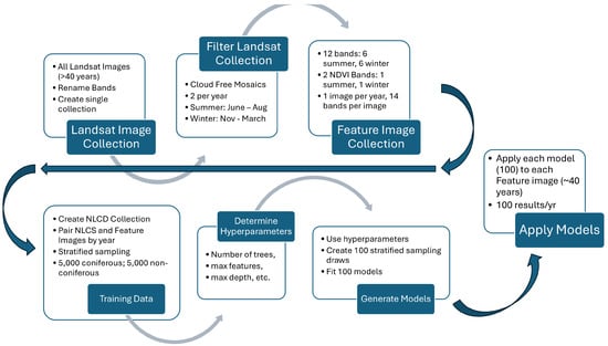
Figure 2. Model creation process chart using 40 years of Landsat images. We created 1 cloud-free mosaic feature image per year with 6 spectral bands and 1 NDVI band for both summer and winter, 14 bands total. We paired feature images with NLCD images and used stratified sampling to generate training data to determine model hyperparameters. We use these hyperparameters with 100 stratified sampling draws to create 100 models, and apply these models to each feature image over the ~40-year study period.

To evaluate changes in coniferous forest coverage for a given year, we sum the pixels classified as coniferous forest class and compute a mean value of the 100 realizations. For discussion and analysis in this paper, we use pixel numbers, though where it is helpful, we provide area values. Pixel numbers can be converted to area measurements by multiplying by the nominal pixel area, 900 m² per pixel (30 m × 30 m).

Our hypothesis is that with sufficient realizations, the area classified as coniferous forest represents the probability distribution of the forest cover in the annual images and provides us with a measure of uncertainty in our modeling. This provides insight into both the extent of coniferous forest coverage as well as the variability and uncertainty in the modeling and classification steps. This approach uses stochastic processes twice, as the RFC model uses stochastically generated decision trees to compute a classification, and we stochastically generate a 100-member ensemble of RFC models based on 100 draws of training data to provide a distribution of pixel classifications for each year.

The following sections provide details on each of the steps and processes.

2.4. Random Forest Classifier

A stochastic process can model physical phenomena where deterministic models are difficult to develop because of natural variation in the process itself, or uncertainty or variation in the driving features of the process. RFCs use a stochastically generated set of decision trees called a “forest” that generally provides higher accuracy than a single, best-fit decision tree model. Each decision tree in the RFC is created using a random subset of features with a random subset of the training data. The RFC aggregates the resulting decision tree models to determine the final classification by majority voting [52]. Each RFC model has five hyperparameters used to fit the model: the number of trees, the maximum number of features considered for splitting a node, the minimum number of leaves to split an internal node, how to split the node, and the maximum number of leaf nodes in each tree.

We created our RFC using a combination of bagging, or stratified stochastic sampling with replacement, to generate the training data. The RFC training process uses random feature selection without replacement to select the features for each tree in the model. As each decision tree in the model only sees a subset of the available features and training data, the individual trees are not prone to overfitting. The majority voting is equally likely to produce a result that is an overestimate of the coniferous forest area as it is to produce an underestimate of the area. We determined the best hyperparameters for our RFC models using randomly selected training data (n = ~5 k) with error metrics computed on the remaining pixels (n = ~2 M). We used these hyperparameters to create a 100-member ensemble of RFC models based on random draws of training data from the 9 years of NCLD/Feature image pairs. We applied these 100 models to each yearly feature image to generate annual estimates of coniferous forest coverage and also to characterize and quantify uncertainty.

We implemented the models using the GEE RFC algorithm, which is part of the GEE platform. As the RFC is part of GEE, we could easily apply the trained models to the complete image collection to generate results, compute the accuracy metrics, and spatially visualize the data. Application of the models within GEE generated a GEE image collection, which contained the model results. We compared these GEE image collections to the NLCD data to compute accuracy estimates. Using GEE allowed us to analyze over 40 years of satellite image data with 100 realizations per year, which is a very large data set, using common computer resources, as the majority of the processing occurred on the GEE.

2.5. Stratified Sampling

Stratified sampling involves dividing the study area data into distinct land cover classes (e.g., forest, urban, water) and then sampling each stratum separately to ensure representative and efficient data collection. The samples are selected from each land cover type (stratum) based on their presence in the study area. This ensures that even rare or less extensive classes (e.g., wetlands) are adequately sampled, preventing them from being underrepresented as they might be in simple random sampling. The number of samples per class can be proportional to class area, equal across classes, or weighted based on specific analysis goals, thereby tailoring representativeness to the study’s objectives. We weighted our samples based on the class area. This approach improves classification accuracy by accounting for variability within each land cover type. We used the GEE stratified sampling algorithms to create our datasets [32].

2.6. Training Image Set

2.6.1. GEE Landsat Images

We accessed Landsat images using the GEE platform. GEE allows users to access and work with large image collections from various sources, including many remote sensing datasets. The available collections include both processed and unprocessed images, along with tools to easily filter image collections. GEE has tools to create mosaics from image collections, including processes that combine images from separate satellite passes or collections, and to build multi-band images where the image bands can include computed data or data from other collections or images. For example, GEE can create a cloud-free mosaic image by selecting image pixels not affected by clouds from all the images in the selected time frame. The user defines the pixel values used in the mosaic; the common methods are either the median cloud-free pixel from the time period or the first cloud-free pixel.

For this study, we wrote a function to collect all the image data from the four Landsat missions (5, 7, 8, and 9) since 1984 into a single GEE image collection [53]. As the missions have slightly different band names, we renamed the bands so that comparable bands across the missions had the same names for ease of processing using approaches from [4,54]. We wrote a preprocessing function to generate cloud-free and snow-free mosaic images for each year, which used the Landsat data quality bands to remove pixels contaminated with either cloud or snow cover. For each year, we created two cloud-free, snow-free mosaic images, one for summer, June to August, and one for winter, September through May. We combined these two mosaic images into a single multi-band image for each year from 1984 to 2024 and added the images to a GEE image collection. This resulted in a new GEE image collection, with one image per year (39 images), each image with 12 bands, i.e., 6 bands for the summer mosaic image and 6 for the winter.

We used Landsat imagery obtained as Level-2 Surface Reflectance products available through GEE. These products are atmospherically corrected and radiometrically calibrated to surface reflectance, ensuring comparability across Landsat missions (Landsat 5 TM, Landsat 7 ETM+, Landsat 8 OLI, and Landsat 9 OLI-2). This preprocessing standardizes spectral values, enabling consistent long-term analysis. Nonetheless, we note known differences in sensor characteristics—particularly between Landsat 7 ETM+ and Landsat 8 OLI—that can affect indices such as NDVI and contribute to variability in results [55,56,57]. Our approach mitigates these differences through calibration inherent in the Level-2 products, but we acknowledge residual discrepancies may remain and discuss their potential influence on our model in the Discussion section. To determine the start and end dates of the summer and winter periods for our study region, we visually examined all the training images for each of the 9 years with NLCD data. We wanted to use these summer and winter periods to better separate coniferous forests from deciduous forests and grasslands by creating image feature data that included both green plants (summer) and dormant plants (winter). We selected cut-off dates that worked well for all 9 years, rather than using year-specific dates, as we wanted to apply these cut-offs to the entire 39-image collection. We visually selected the period from June to August to create the summer mosaic images, and the period from September of the previous year through May of the current year to create the winter mosaic image. This large range allowed two complete cloud-free, snow-free mosaic images to be generated for each year. We used the minimum cloud-free, snow-free pixel value to create the winter mosaics, and we used the maximum cloud-free pixel value for the summer mosaics. This provided good contrasts among the land covers and allowed us to better distinguish coniferous forest coverage.

2.6.2. Labeled Data

The United States Geologic Survey (USGS) has been providing the NLCD every few years since 2001, which classifies land cover over the United States [50]. This dataset is available through GEE. We used these NLCD images to develop labeled data to train our model and to assess model accuracy. The USGS has released 9 datasets that were available as of the initial writing of this paper. NLCD data are available for the years 2001, 2004, 2006, 2008, 2011, 2013, 2016, 2019, and 2021 [51]. The USGS states that their NLCD has varied in accuracy, but is now 91.1% accurate [51]. The NLCD 2016 land cover product achieved improvements in classification accuracy, with Level II and Level I overall accuracies reaching 86.4% and 90.6%, respectively—representing a 5% increase from the 2011 dataset [58]. This high level of accuracy was maintained in the NLCD 2019 release, as confirmed by its own accuracy assessment [59]. The USGS has recently, since the start of our analysis, released a complete NLCD dataset covering the entire Landsat period, back to 1984. Since we are interested in classifying high-elevation coniferous forests and do not want to include sparse cover such as that by pinyon (Pinus edulis) and juniper (Juniperus osteosperma) forests, we used the available 9-year NLCD data and did not redo the analysis with the additional NLCD data. As noted, our models for the high-elevation regions in our study area have similar accuracy to the stated NCLD accuracy. As we are most interested in trends, we hold that our approach is appropriate. Since this work has been completed, the USGS has released NLCD data covering the entire Landsat collection period since 1984. This dataset is not useful for evaluating dense coniferous forest change, as it also includes sparse pinyon (Pinus edulis) and juniper (Juniperus osteosperma) forests in the west. We felt there would be little benefit in extending the training data to include all ~40 years, where the previous NLCD data set for 9 years is approximately 25% of the total—a reasonable training split.

2.6.3. Feature Selection

We needed to select potential model features that could be used to classify dense coniferous forest coverage at higher elevations. By “dense”, we mean that pixels classified as “coniferous” have approximate full pixel coverage of evergreen trees. As noted earlier, pinyon (Pinus edulis) and juniper (Juniperus osteosperma) forests have individual trees often widely dispersed, often with a pixel containing a single tree. These are generally classified as coniferous in the NLCD datasets.

Visually, it is difficult to distinguish between coniferous forest coverage from deciduous trees, shrubs, or grasslands in the summer because they all are fully foliated and appear similar in remote sensing data. Because coniferous trees keep their foliage year-round and deciduous trees, shrubs, and grass lose their leaves or pigment in the winter, we assumed that using a combination of features that included data collected during winter and summer seasons would increase the model’s ability to separate the coniferous from other vegetative classes. To create these features, we created an image for each year built from two cloud-free, snow-free mosaiced Landsat images, one from the summer and one from winter. For each of these mosaic images, we retained six multi-spectral Landsat bands, bands 2–7 (blue, green, red, near-infrared, short-wave infrared 1, and short-wave infrared 2), then combined the two images into a single multi-band image, one image per year. This resulted in an image collection with 1 image per year with 12 bands, 6 bands that represented the summer mosaic, and 6 that represented the winter mosaic.

For feature selection, we created an individual model for each of the 9 years with NLCD data and evaluated the importance of different potential features. For feature selection, we created models with various features using stratified sample data (~100 s of pixels), then evaluated accuracy on the remaining image data (~2 M pixels)

We evaluated many features, including all possible normalized band difference ratios, band ratios, inverse band values, and log band values. Our analysis showed that most of these features did not improve model accuracy. We found that one of the normalized band difference ratios, the Normalized Difference Vegetation Index (NDVI), did improve model accuracy for each of the 9 test years.

NDVI is commonly used in remote sensing to identify vegetation [25,26,60] and is the normalized difference of the red (RED) and near infrared (NIR) bands:

$$\mathrm{N}\mathrm{D}\mathrm{V}\mathrm{I}={\displaystyle \frac{(\mathrm{N}\mathrm{I}\mathrm{R}-\mathrm{R}\mathrm{E}\mathrm{D})}{(\mathrm{N}\mathrm{I}\mathrm{R}+\mathrm{R}\mathrm{E}\mathrm{D})}}$$

(1)

The NDVI can distinguish between different land covers, but with low specificity. We found that including it in our feature set contributed significantly to model accuracy. For example, even in the summer, coniferous trees have a different range of NDVI values than grasslands, but there is enough variation and overlap that it is difficult to separate these two landcover classes based only on NDVI. For our model feature set, we computed NDVI values for both the summer and winter time periods. NDVI seasonal changes are significant for deciduous trees and most plants, as they lose their leaves or chlorophyll in the winter [61,62].

For the final model training image collection, we used GEE to combine the 12-band summer and winter mosaic images along with the summer and winter computed NDVI values into a 14-band image, then added the NCLD land cover band to create the final 15-band training image.

The final image collection, with 9 images, had 12 multi-spectral Landsat bands, 6 bands for summer and 6 for winter, and 2 NDVI bands, one for summer and one for winter. These multi-spectral bands were 2–7 (blue, green, red, near-infrared, short-wave infrared 1, and short-wave infrared 2). This resulted in nine images with 14 feature bands and one training band, 15 bands total. Thus, the 9-image collection included images where the first 14 bands are the model features, and the last band is the model target, one for each year that has NLCD data (i.e., 2001, 2004, 2006, 2008, 2011, 2013, 2016, 2019, and 2021). We used this image collection to determine hyperparameters and then train the 100-member ensemble of RFC models.

For model applications, we created an image collection with one image per year from 1984 to 2024, where each image in the collection contained 14 bands or features.

2.6.4. Model Training Data

Because of the large study area and memory and computational constraints, even using GEE resources, we could not use all the pixels in the selected region to train our models. Rather, we used stratified sampling to stochastically select pixels for the training data set [29,63,64,65]. We applied the stratified sample function from GEE to extract data points within our study area for each of the 9 years in the training data set [32]. Each selected data point contained all 15 band values, i.e., 14 features and one target value. The GEE stratified tool selects pixels that provide a uniform distribution of samples from each of the categories provided. For our data, from each image, we extracted 38 samples from each of the 15 different NLCD landcovers—one of which is our desired landcover, evergreen forest. This gave a total of 513 samples per image, or 5130 training samples over the 9 years of training data. We used the remaining ~2 M pixels per image for accuracy metrics.

We used single draws of 5130 pixels for feature and hyperparameter selection for our model training. For each test run, with either different features or hyperparameters, we computed accuracy across the entire 9-image collection using approximately 20 M pixels.

We recognize that relying solely on NLCD classifications introduces potential biases, as these are themselves satellite-derived products. While no independent field data were available for this study, our approach leverages ensemble modeling and multi-year validation to mitigate these limitations, and future work will incorporate ground-based or higher-resolution reference data (e.g., NAIP imagery) to strengthen calibration.

2.7. Model Development

2.7.1. Hyperparameter Determination

The GEE RFC model requires the selection of six hyperparameters: the number of decision trees, the number of variables per split, the minimum leaf population, the bag fraction, the number of max nodes, and a seed, which allows subsequent model runs to use the same statistical draws. We performed an ad hoc analysis of these parameters with perturbations around the default values. We found that the impact of adjusting the default parameter values on model results was minimal, so we used default values for all the parameters except the number of trees in the model. While the number of trees did have a slight impact on model accuracy, it was not large and was significantly lower than the accuracy variation across the 9 years of training data. For the final models, we selected 20 as the number of trees because it provided good results while still running quickly with all other values as default.

After determining the model hyperparameters, we created 100 different RFC models using the GEE stratified sampling tool to generate 100 draws of 5130 training points per draw from the 9 years of training images. We fit a model on each of these 100 draws. The resulting 100 models used 51,300 stochastically selected training points. The points were selected with replacement, so some may have been duplicated, but the population of potential points was 10 million pixels (~2 M pixels per image with 9 images), so we assume there was little repetition.

2.7.2. Accuracy Assessment

To evaluate the accuracy of the final trained model ensemble, we applied the 100-model ensemble to the complete 9-year image collection and classified each pixel. We then compared our classification with the NLCD landcover image for each year. The subbasin we used for this study is high elevation, and the conifers are generally fir and spruce with dense coverage. This allowed us to use every pixel in the image for accuracy computation. For this validation task, the models were trained on 5130 data points with accuracy evaluated at approximately ~20 M pixels, or ~2 M for each year. As we are only interested in the accuracy of the evergreen class, we evaluated classification accuracy on pixels labeled as evergreen pixels in both the model and NLCD images for each of the 100 ensemble runs. We did not evaluate other classes, as our model was only trained for binary classification.

To help understand model variation and accuracy, we used K-fold cross-validation implemented in GEE and applied it to the final 100-member model ensemble [66,67]. We used 5 folds of the 100-member model ensemble, which meant that the accuracy results are based on 500 model runs. This approach provided good accuracy estimates because of the large number of runs and the large number of pixels used for evaluation (~20 M).

To evaluate model performance, we report several accuracy metrics using the ~20 M pixels from the ensemble runs. These metrics include the Model Average, which is the mean coniferous forest pixel count predicted across the ensemble runs for a given year; the Model Median, which is the central value of those predictions, and is less sensitive to extreme realizations; the Percent Difference, which compares model results (both the average and median values) to the NLCD reference value, indicating relative over- or underestimation; and finally, the Standard Deviation, which quantifies the spread of model predictions across the ensemble, providing a measure of uncertainty for each year

In addition to computing accuracy metrics, we conducted a visual comparison of our model results with the NLCD data to determine if there were spatial trends or patterns in prediction errors between the model and the NLCD data. For the visual analysis, from the 100-member ensemble, we selected the run with the results closest to the ensemble average and generated difference images between the model-generated classification and the NLCD dataset for each of the 9 years. These different images labeled each pixel with one of three values: no-change (our model matched the NLCD data), classified as evergreen by our model but not by the NLCD, or classified as evergreen by the NLCD but not by our model. This allowed us to both assess the accuracy of the model and identify spatial or pattern trends in accuracy.

2.8. Final Model Description

We trained the final 100-model ensemble using 100 draws of stratified samples from the entire 9 years of NLCD data, each draw including data from all 9 years. This generated 100 training sets, with each training dataset containing 5130 samples, with each sample consisting of the 14 features based on Landsat images and the label from the NLCD.

Our final ensemble models used 20 trees, 23 as the maximum number of features considered for splitting a node, 1 as the minimum number of leaves to split an internal node, 0.5 as the fraction of input to bag per tree, and no maximum number of leaf nodes in each tree. We applied the trained 100-member model ensemble on each year of Landsat data from 1984 to 2024, as a “year” in our data goes from September of the previous year to August of the current year; our results start in 1986.

To present the results, we used several methods. We provide box-and-whisker plots for each year to show trends along with model variation. For spatial visualization, we used the 1987 image as the base and computed changes in evergreen coverage from 1987. As shown in later discussions, 1986 seemed anomalous, so we used 1987 as the base year. For visual analysis, we labeled each pixel with the change in coniferous coverage from 1987, with white for no change, red for coniferous in 1987 but not in the current year, and green for coniferous in the current year but not in 1987. This representation allowed us to visually identify and discuss spatial trends in coniferous forest coverage.

3. Results and Discussion

3.1. Accuracy

Figure 3 and Table 1 display the results of the K-fold cross-validation on the 100-member model ensemble applied to the 9 years of NLCD training data. It presents model accuracy as boxplots of predicted coniferous forest cover compared to NLCD reference values, with the spread indicating variability across ensemble runs and red bars showing NLCD estimates. Figure 2 shows the model result distributions for each year, with the NLCD coniferous forest coverage value for the year shown as a red bar. Table 1 provides statistical measures of accuracy for each of the 9 years using average and median predicted pixel counts, percent difference from NLCD reference values, and the standard deviation across ensemble runs as an uncertainty estimate. These results are based on a large test data set, 500 runs per year, with accuracy computed on the remaining ~2 M pixels for each year. We present these results in pixel counts, rather than area, as that provides more insight into model performance.

Figure 3. Cross-validation box plots of model-predicted forest cover vs. the NLCD values for the year in units of pixels. These are based on a 5-fold cross-validation of the 100-member model ensemble. Data are presented in pixel counts rather than area to highlight model performance. Single dots are data outside 1.5 * the interquartile range (1.5*IQR).

Table 1. Model Average, Median, Mean, and Median Percent Difference from NLCD data, and Standard Deviation computed using 5 K-fold cross-validation on the 100-member model ensemble. Data are presented in pixel counts rather than area to highlight model performance.

Year	NLCD	Model Average Values	Percent Difference (Average Values)	Model Median	Percent Difference (Median)	Standard Deviation of Model Values
2001	473,153.0	452,515.9	−4.36%	452,556.5	−4.35%	10,848.7
2004	473,182.0	475,443.1	0.48%	474,701.5	0.32%	9326.2
2006	472,937.0	497,944.3	5.29%	498,435.0	5.39%	8950.7
2008	472,897.0	525,865.0	11.20%	524,915.0	11.00%	13,976.8
2011	469,830.0	496,917.1	5.77%	497,494.0	5.89%	8982.0
2013	470,040.0	444,369.8	−5.46%	444,368.0	−5.46%	9415.5
2016	469,173.0	640,625.8	36.54%	639,515.5	36.31%	27,635.1
2019	469,657.0	612,250.6	30.36%	612,444.5	30.40%	14,019.1

The results from this validation exercise show that the model results from 2001 to 2013 are fairly accurate with small variations, with all but 2008 having differences less than 6%, while 2008 has an 11% difference. However, 2016 and 2019 had poor results, with differences from the NLCD data of approximately 137% and 30%, respectively (Figure 3 and Table 1). The standard deviations for 2001, 2004, 2006, 2008, and 2011 are all between approximately 9000 and 10,000 pixels, while 2008 and 2019 have standard deviations of approximately 14,000 pixels, with 2016 having the largest standard deviation of approximately 27,000 pixels. While these seem large, each image contains over 2,358,546 pixels. From a percentage standpoint, these standard deviation values range from 0.379% to 1.17% of the total pixels for 2006 and 2016, respectively. In general, model differences from the NLCD data for the coniferous class are on the same order of magnitude as those reported for the NLCD dataset [51,58,59].

3.2. Spatial Validation

To visually evaluate spatial accuracy, we produced change maps using the model results for two years, comparing the median 100-member ensemble model results with NLCD data in 2001 and 2019 (Figure 4). We selected these two years as 2001 slightly underpredicts the amount of coniferous forest coverage (Figure 3), while the 2019 model predicts significantly higher coniferous forest coverage than the NLCD data set (Figure 3). In Figure 4, white represents pixels classified the same in both data sets, green represents pixels classified as coniferous forest in our model but not the NLCD data, and red represents pixels classified as coniferous forest in the NLCD data but not in our model.

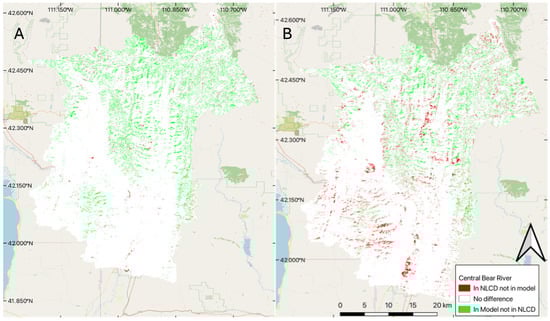
Figure 4. Difference between the NLCD and the model for two selected years: (A) difference for 2001, and (B) difference for 2019.

The differences between the two approaches appear to follow dendritic patterns that we would expect to see, as NLCD data often misclassifies coniferous forest, confusing it with shrubs and deciduous forest, especially for darker pixels on shadowed ridges and steep hillsides, something we tried to address by using features based on winter images in our model feature set. For 2001, we see a few pockets of coniferous forest cover (red) that do not follow this pattern, which could indicate inaccuracy in the trained data, but overall, the trained model performed very well, especially in 2001. Panel B (Figure 4), 2019 comparison, shows larger differences, especially in the southern portion of the basin, which is lower in elevation and has less coniferous forest, and likely many of the areas classified as coniferous forest are pinyon (Pinus edulis) juniper forest, rather than dense spruce/fire forest. These results support Stehman’s [28] findings, where they found the level 1 accuracy of NLCD 1992 to be 80 percent and the level 2 accuracy to be 46 percent. Meaning that the 1992 data was very accurate when it came to identifying forests, but not as accurate at separating the deciduous from the coniferous forest cover. This implies that we would expect to see a consistent dendritic pattern (representing the forest cover in the valleys of the mountains), but large variability between the identification of the forest types (showing up as green and red pixels within the dendritic pattern). This is especially true as we are subdividing coniferous forests to exclude pinyon (Pinus edulis) and juniper (Juniperus osteosperma) stands. We hypothesize that using both summer and winter features addresses that issue in our model and provides more accurate results, but we do not have ground truth to quantify or support that statement.

The right panel (B) of Figure 4 shows that in the bottom (south) part of the basin, the NLCD data indicates a number of coniferous forest pixels classified as coniferous by the NLCD data, but are not classified as forest by our model. This part of the basin does not have a significant amount of coniferous forest (Figure 1) but does have deciduous trees and is lower in elevation, which also includes pinyon (Pinus edulis) and juniper (Juniperus osteosperma) coverage. We attribute the 2019 differences in the southern part of the basin to NLCD data classifying deciduous trees and pinyon (Pinus edulis) and juniper (Juniperus osteosperma) forest as coniferous forest coverage. As this result significantly varies with the year, we expect the main contributing factor to be the deciduous forests being misclassified. While we do not have ground truth, we believe that our model is doing better in this region than the NLCD data. We attribute this to the winter features we used to train the model, which better discriminate coniferous trees, and the fact that we do not consider pinyon (Pinus edulis) and juniper (Juniperus osteosperma) in the dense coniferous class, while the NCLD does include this land cover type in the coniferous forest end member. The training data most likely also included some misclassified pixels from the NLCD dataset, but most of the training data were coniferous, and it is likely the model used the clear differences between deciduous and coniferous forests in the winter to more accurately classify the pixels. These differences in the NLCD data could be a cause of the larger model variability in this time frame, as some of the training data are misclassified.

3.3. Long-Term Coniferous Forest Coverage Change

Figure 5 displays the results of applying our model to the complete 40-year Landsat dataset starting in 1984 and continuing to 2024. The results are labeled from 1986 due to when the year starts, with the winter images from the preceding year. The plots are box-and-whisker plots, where the box ends represent the 25th and 75th percentiles and the whisker ends represent 1.5*IQR (interquartile range) outliers, which are values beyond 1.5*IQR, shown as individual dots. The results generally follow what we would expect: a gradual increase in the coniferous forest cover over time. A linear fit to the data (Figure 5) shows a change from approximately 360 km² (400,000 pixels) of coniferous forest in 1985 to approximately 620 km² (680,000 pixels) in 2024, an increase of 65% over 40 years (Figure 5). If we use 1987 as the base year, as 1986 appears to be too high, the increase from 1987 to 2024 goes from 325 km² (360,000 pixels) to 775 km² (85,000 pixels), which is an increase of about 130%. If we use 1986 as the base year with an area of 425 km² (47,000 pixels), then the increase is about 82%. There are notable outlying years, and the ensemble prediction range in any given year is relatively large. In particular, the estimated coniferous forest coverage in the years 1996 and 1998 is high compared to both previous and subsequent years, while the years 2013 to 2019 have lower results than previous and subsequent years. The results from 2015 and 2016 are well above the linear fit to the data, though they generally follow the expected trend. The variance in the results, as shown by the size of the box-and-whisker symbols in the plots (Figure 5), increases in 2014 with the addition of the Landsat 8 data. We believe this increase in variance is because of the known differences between Landsat 8 and the previous missions. After Landsat 9 data became available in 2021, this variance seems to decrease, and the increasing trend in coniferous coverage is again apparent. While there are anomalous years and variance in the ensemble predictions, the long-term trend is apparent and significant, with coniferous forest coverage approximately doubling over the 40-year study period. While the results show an overall trend of increasing coniferous forest cover, different periods exhibit different rates. These periods are discussed in more detail in Section 3.6.

Figure 5. Model results of coniferous forest cover area through time with a linear trend line included. This is a box-and-whisker plot, where the box ends represent the 25th and 75th percentiles and the whisker ends represent 1.5*IQR (interquartile range).

The box plots show that variance or uncertainty is generally larger for the two anomaly results for the years 1996 and 1998, and since 2014, when Landsat 8 data became available. Some of this variance could be because the annual mosaic images can contain data from either Landsat 7 or Landsat 8, with differences between the two collections. In addition to variance significantly increasing after 2014 with the availability of Landsat 8 data, there is no general trend in variability, with 2014 and 2015 having higher median values than the historical trend and 2018 and 2019 being generally lower, with the intervening years generally following the long-term linear trend. We attribute this increased variance to mixing data from Landsat 7 and Landsat 8. We do not see similar variance increases in 1999, when we have mixed data from Landsat 5 and Landsat 7, or 2018, when we have mixed data from Landsat 7 and Landsat 8. The data after 2021, when Landsat 9 data becomes available, demonstrates large variance or uncertainty in any given year, as shown by the size of the whisker plots, but the year-to-year trend shows a linear trend in the median, with less deviation in the early years of the data.

3.4. Spatial Changes

Because the change quantification methods do not provide a way to characterize or describe spatial distributions and correlations, we spatially compared the model results of change in coniferous forest coverage for selected years (Figure 6). We use 1987 as the base year, and provide change maps for 1994, 2001, 2008, and 2016. In these change maps (Figure 6), a red pixel indicates that evergreens were present in 1987, but not in the later years, representing a decrease in coniferous growth at that pixel. Green is the inverse, indicating the pixel classified as coniferous in the later years and not in 1987, representing an increase in coniferous growth through time. White indicates no change in coniferous classification of the pixel.

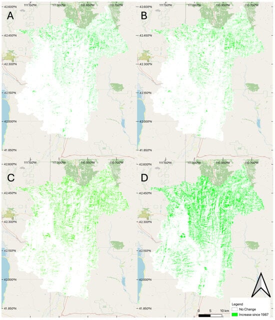
Figure 6. Change maps (differences) between 1987 and selected years. (A) differences from 1987 to 1994. (B) differences between 1987 and 2001. (C) differences between 1987 and 2016. (D) differences between 1987 and 2024.

The change maps from 1987 in Figure 6 show increasing coniferous forest coverage over time, generally with some small areas losing coverage. Figure 6 shows that the differences in 1991 and 2001 are similar. Using 1987 as the base, coniferous forest coverage significantly increased by 2024 (Figure 6 Panel D), with the changes in the mountainous portions of the basin as expected. Most of the increase in coniferous coverage is in the higher elevations in the northern part of the basin. As shown by the sequence from Figure 6A–D, coniferous coverage in the northern portion of the basin shows a visible increase following patterns we expect for forest growth.

3.5. Landcover Change Trends

Figure 7 displays the annual results from the ensemble model classification of coniferous forest cover from 1986 to 2024 as box-and-whisker plots. We visually fit trend lines to this data to identify change periods and how forest coverage changed over these periods. The green lines represent periods with increases in coniferous cover; the red lines are periods with a decrease in coniferous land cover; and the grey lines represent periods with little change in coniferous forest cover. We fit these lines visually. The seven years circled in red are outliers. We consider a year to be an outlier if the whisker (1.5× the interquartile range) does not overlap the results from both the previous and following years’ data. In cases where an outlier was found before or after the point, we looked at the data on the other side of the outlier. For example, we did not consider the year 1997 an outlier because its spread overlapped with 1995 and appears to overlap with 1999, even though it did not overlap with either 1996 or 1998. On the other hand, we considered 1996 and 1998 as outliers because even though they overlap with each other, they do not overlap with 1994 through 2000.

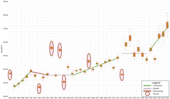
Figure 7. Model-predicted evergreen forest cover by year with apparent trend lines and anomalies. The general trend continues through 2024, but the period from 2013 to 2021, marked as “steady”, shows considerable variation.

Between 1986 and 2012, we identified three periods of increasing coniferous coverage (1986–1991, 2001–2012, and 2021–2024), one period of decreasing coniferous coverage (1991–1995), and two periods of stability (1995–2001 and 2013–2019). We also identified six outliers from 1986 to 2013 (1986, 1993, 1996, 1999, 2005, 2013). The results from 2014–2024 appear to be different than the results from 1986 to 2013 in two ways: (1) they have large spreads or variance in the ensemble model results, many years approaching 100,000 pixels, and (2) they show high variability from year to year but do not meet the standard for an outlier identified earlier because of their large spreads, which overlap previous and post years. We are unsure of the reason for the change, but a few possibilities are worth exploring, such as a mix of satellite data and the images from which pixels were selected for the composite mosaic used for the model features. Though there is large variability, we classified the period from 2013–2019 as steady, and the period from 2019–2024 as increasing.

3.6. Potential Issues

The data contains years that appear to have incorrect data, as they do not fit general trends, and we would not expect large changes in coniferous coverage year to year. Unfortunately, we do not have ground truth to verify issues with the models. The first possibility for these issues is that the model that we trained, which we assumed measured coniferous forest cover, is in reality tracking some other factor that can exhibit large year-to-year changes. For model validation, we compared the results to the NLCD for the available years. We obtained fairly accurate results with an approximate 10 percent difference between our prediction and NLCD’s prediction. We used this to justify our model. The problem is that if our model is predicting a measure that generally correlates with coniferous forest cover but in reality is something else, it would be difficult to identify or quantify this issue unless the predicted results were unreasonable or impossible. For instance, from 1995 to 1997, our model predicted an evergreen cover of ~52.3 km² (~570,000 pixels) in 1995 to ~61.2 km² (~680,000 pixels) in 1996, back to ~50.4 km² (560,000 pixels) in 1997. It is not likely that we would see this pattern in forest cover, but it is possible that we could see this pattern in confusing land cover types, such as shrubs, grasslands, or deciduous forest, which could be caused by changes in precipitation or temperature or selecting different pixels for the composite mosaic used for model features. Weather patterns could also cause issues, such as causing deciduous trees to be green longer or present differently, causing bushes or shrubs to confuse the model. This type of confusion could also occur in warm years when the cloud-free, snow-free mosaic image selected pixels for the training data before the leaves fell. The second possibility is our creation of summer and winter features, where we selected the first “good” pixels in the time period. For years with anomalous weather, this approach could result in anomalous pixels. This could be potentially alleviated by selecting the median pixel, but for years with significant snow coverage, the median pixel may be impacted by snow coverage.

These issues are difficult to characterize without exploring every possible influencing factor. However, one of the most likely causes is precipitation differences or changes over the years. To explore this issue, we evaluated the possibility that the model was predicting precipitation instead of coniferous cover. While Landsat images cannot record precipitation, they can track the effects of precipitation and temperature on the land cover. In times of higher precipitation, we would expect to see more green or greener vegetation in the images. This could directly influence the classification of coniferous forest coverage by creating conditions that reflect the evergreen cover conditions. Alternatively, drought conditions make much of the landscape brown, making the contrast between evergreen and other covers more pronounced, resulting in less area being classified as coniferous forest.

Utah’s Division of Natural Resources (DNR) has tracked the precipitation totals for the basins in Utah and provided charts of the precipitation by year over the study period (Figure 8). Their annual total data runs from October of the previous year to September of the year listed. This time frame follows closely with the dates we used for our predictions, which ran from September of the previous year to August of the year listed. Visually comparing precipitation over time, we do not see a correlation between the precipitation measured during the year and the evergreen forest classification. These data provide no indication of conditions that would result in higher classifications of coniferous forest when less rainfall occurs, as well as no indication of higher coniferous classifications during years of more precipitation. There is no increasing or decreasing trend tied to precipitation above or below the average. There appears to be no correlation between precipitation and our models’ predictions, making it unlikely that the model is reflecting precipitation over evergreen cover.

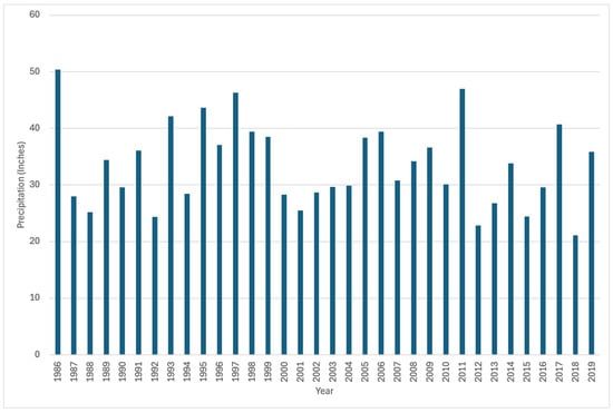
Figure 8. Precipitation in the Bear River Upper Bear. Data from Utah’s Division of Natural Resources (DNR).

Another possibility is that the data from the different Landsat satellites are affecting the model due to differences in sensor behavior. Landsat 8 began collecting data in 2013, which is the same time that our data starts to exhibit increased variability in our predictions, indicating the possibility that the data from Landsat 8 is affecting our results. Landsat 9 started collecting data in 2021, and our data shows more apparent trends and less variability after this period, though this period includes a mix of Landsat 8 and 9 data. A study by Holden and Woodcock explored the differences in images between Landsat 7 and Landsat 8 [55]. They found that the blue, green, and red bands in Landsat 8 were consistently darker than the same bands in Landsat 7. Conversely, they found that the near infrared band was lighter in Landsat 8 than in Landsat 7. This finding could be a major contributing factor to the increased spread we see in the data after 2013, when Landsat 8 data were part of the image collections. Eight of the ten bands that we used as our training data, according to Holden and Woodcock [55], have consistent differences between Landsat 7 and Landsat 8 images [55]. Roy et al. [57] came to similar conclusions, noting that Landsat 8’s bandwidth for its bands is narrower than Landsat 7’s bandwidths for the same bands. This also could play a role in the increased variability of the predictions.

Roy et al. [57] assert that NDVI calculated using Landsat 8 produces higher values for NDVI than using Landsat 7 images. A higher NDVI value would result in more pixels being identified as coniferous, which would result in higher pixel counts using Landsat 8. This is a likely reason that we see an increase in the pixel count in 2014. The decrease in pixel count that we see in 2013 is likely the result of the model using a mixture of Landsat 7 and 8 data. Since the winter values were taken from Landsat 7, they would appear normal to the model but would be smaller than the summer values taken from Landsat 8. This change in NDVI value from winter to summer would reflect what we would expect to see from deciduous trees, thus reducing the number of pixels identified as coniferous forest. Our method of generating cloud-free, snow-free mosaics used pixels from either the Landsat 7 or 8 missions in the feature dataset and did not distinguish between the missions. It is likely that the selection methods preferred pixels from different Landsat missions in the mosaic images, as we used the maximum pixel for the summer mosaic and the minimum pixel for the winter mosaic. This means if there was a cloud-free, snow-free pixel, our method would choose a Landsat 7 pixel for the summer features and a Landsat 8 pixel for the winter features. While variability in the results increases, the general trends remain constant, and we hold that our approach is valid for evaluating long-term change in coniferous forest coverage. In addition, we used calibrated reflectance data (Level 2, Tier 2 data process data available from GEE), which minimizes the differences between the Landsat missions, as the issues with band calibration are considered when creating the processed products.

4. Conclusions

We demonstrate a stochastic framework for classifying high-elevation coniferous forests using Landsat imagery and Random Forest models. By generating a 100-member ensemble, we quantified both long-term forest cover change and associated uncertainty. Results indicate a substantial increase—approximately a doubling—of dense coniferous cover in the Central Bear River subbasin since the mid-1980s, from ~350 km² (1986) to over 750 km² (2024), with standard deviations per year ranging between 0.38% and 1.2%. The greatest expansion occurred at higher elevations in the northeastern basin.

The approach addresses limitations of the NLCD by distinguishing dense spruce–fir forests from sparse pinyon–juniper stands, yielding estimates more relevant for hydrologic analysis. Model accuracy was generally high (>94% in most years), though variability increased after 2013, coinciding with the transition to Landsat 8, highlighting the influence of sensor differences on long time series. We found that the model produced accurate results using images from Landsat 5, 6, and 7. The model did not perform as well when we used images from Landsat 7 and Landsat 8 (starting in 2013) and seemed to do better with mixed Landsat 8 and Landsat 9 data after 2021. The model predicted more forest cover with a wider variability in the predictions using Landsat 8 images than using Landsat 5, 6, and 7 images. We believe that this is because of changes in the sensors between the Landsat 7 and 8 missions.

Our findings have implications for water resources in the Great Salt Lake watershed: a ~65–130% increase in coniferous cover over 38 years suggests greater snow interception and sublimation, and therefore reduced infiltration and runoff. The framework is adaptable to other land-cover classes and regions, providing a scalable method for long-term monitoring with explicit uncertainty estimates.

We hold that our model is more accurate than the NLCD data in classifying dense coniferous forest because we used features based on both summer and winter images, even though we used NLCD data for training labels, which also includes pinyon (Pinus edulis) and juniper (Juniperus osteosperma) forest in this region. We plan to use high-resolution National Agriculture Imagery Program (NAIP) imagery as ground truth in a future study to better analyze and quantify this issue.

References

- Zhu, Z.; Woodcock, C.E. Continuous change detection and classification of land cover using all available Landsat data. Remote Sens. Environ. 2014, 144, 152–171. [Google Scholar] [CrossRef]
- Hansen, M.C.; Loveland, T.R. A review of large area monitoring of land cover change using Landsat data. Remote Sens. Environ. 2012, 122, 66–74. [Google Scholar] [CrossRef]
- Zhao, Y.; Feng, D.; Yu, L.; Cheng, Y.; Zhang, M.; Liu, X.; Xu, Y.; Fang, L.; Zhu, Z.; Gong, P. Long-term land cover dynamics (1986–2016) of Northeast China derived from a multi-temporal Landsat archive. Remote Sens. 2019, 11, 599. [Google Scholar] [CrossRef]
- Tanner, K.B.; Cardall, A.C.; Williams, G.P. A Spatial Long-Term Trend Analysis of Estimated Chlorophyll-a Concentrations in Utah Lake Using Earth Observation Data. Remote Sens. 2022, 14, 3664. [Google Scholar] [CrossRef]
- Wulder, M.A.; Roy, D.P.; Radeloff, V.C.; Loveland, T.R.; Anderson, M.C.; Johnson, D.M.; Healey, S.; Zhu, Z.; Scambos, T.A.; Pahlevan, N. Fifty years of Landsat science and impacts. Remote Sens. Environ. 2022, 280, 113195. [Google Scholar] [CrossRef]
- Phiri, D.; Morgenroth, J. Developments in Landsat land cover classification methods: A review. Remote Sens. 2017, 9, 967. [Google Scholar] [CrossRef]
- Potapov, P.; Hansen, M.C.; Kommareddy, I.; Kommareddy, A.; Turubanova, S.; Pickens, A.; Adusei, B.; Tyukavina, A.; Ying, Q. Landsat analysis ready data for global land cover and land cover change mapping. Remote Sens. 2020, 12, 426. [Google Scholar] [CrossRef]
- Manandhar, R.; Odeh, I.O.; Ancev, T. Improving the accuracy of land use and land cover classification of Landsat data using post-classification enhancement. Remote Sens. 2009, 1, 330–344. [Google Scholar] [CrossRef]
- Hawbaker, T.J.; Vanderhoof, M.K.; Schmidt, G.L.; Beal, Y.-J.; Picotte, J.J.; Takacs, J.D.; Falgout, J.T.; Dwyer, J.L. The Landsat Burned Area algorithm and products for the conterminous United States. Remote Sens. Environ. 2020, 244, 111801. [Google Scholar] [CrossRef]
- Hawbaker, T.J.; Vanderhoof, M.K.; Beal, Y.-J.; Takacs, J.D.; Schmidt, G.L.; Falgout, J.T.; Williams, B.; Fairaux, N.M.; Caldwell, M.K.; Picotte, J.J. Mapping burned areas using dense time-series of Landsat data. Remote Sens. Environ. 2017, 198, 504–522. [Google Scholar] [CrossRef]
- Vanderhoof, M.K.; Fairaux, N.; Beal, Y.-J.G.; Hawbaker, T.J. Validation of the USGS Landsat burned area essential climate variable (BAECV) across the conterminous United States. Remote Sens. Environ. 2017, 198, 393–406. [Google Scholar] [CrossRef]
- DeVries, B.; Huang, C.; Armston, J.; Huang, W.; Jones, J.W.; Lang, M.W. Rapid and robust monitoring of flood events using Sentinel-1 and Landsat data on the Google Earth Engine. Remote Sens. Environ. 2020, 240, 111664. [Google Scholar] [CrossRef]
- Sivanpillai, R.; Jacobs, K.M.; Mattilio, C.M.; Piskorski, E.V. Rapid flood inundation mapping by differencing water indices from pre-and post-flood Landsat images. Front. Earth Sci. 2021, 15, 1–11. [Google Scholar] [CrossRef]
- Markert, K.N.; Williams, G.P.; Nelson, E.J.; Ames, D.P.; Lee, H.; Griffin, R.E. Dense Time Series Generation of Surface Water Extents Through Optical–SAR Sensor Fusion and Gap Filling. Remote Sens. 2024, 16, 1262. [Google Scholar] [CrossRef]
- Rostami, A.; Chang, C.-H.; Lee, H.; Wan, H.-H.; Du, T.L.T.; Markert, K.N.; Williams, G.P.; Nelson, E.J.; Li, S.; Straka, W., III. Forecasting Flood Inundation in US Flood-Prone Regions Through a Data-Driven Approach (FIER): Using VIIRS Water Fractions and the National Water Model. Remote Sens. 2024, 16, 4357. [Google Scholar] [CrossRef]
- De Sa, N.C.; Carvalho, S.; Castro, P.; Marchante, E.; Marchante, H. Using landsat time series to understand how management and disturbances influence the expansion of an invasive tree. IEEE J. Sel. Top. Appl. Earth Obs. Remote Sens. 2017, 10, 3243–3253. [Google Scholar] [CrossRef]
- Valero-Jorge, A.; González-De Zayas, R.; Matos-Pupo, F.; Becerra-González, A.L.; Álvarez-Taboada, F. Mapping and monitoring of the invasive species Dichrostachys cinerea (Marabú) in central Cuba using Landsat imagery and machine learning (1994–2022). Remote Sens. 2024, 16, 798. [Google Scholar] [CrossRef]
- De Jong, S.M. Derivation of vegetative variables from a Landsat TM image for modelling soil erosion. Earth Surf. Process. Landf. 1994, 19, 165–178. [Google Scholar] [CrossRef]
- De Asis, A.M.; Omasa, K. Estimation of vegetation parameter for modeling soil erosion using linear Spectral Mixture Analysis of Landsat ETM data. ISPRS J. Photogramm. Remote Sens. 2007, 62, 309–324. [Google Scholar] [CrossRef]
- Pickup, G.; Nelson, D. Use of Landsat radiance parameters to distinguish soil erosion, stability, and deposition in arid central Australia. Remote Sens. Environ. 1984, 16, 195–209. [Google Scholar] [CrossRef]
- Brandão, A.O., Jr.; Souza, C.M., Jr. Mapping unofficial roads with Landsat images: A new tool to improve the monitoring of the Brazilian Amazon rainforest. Int. J. Remote Sens. 2006, 27, 177–189. [Google Scholar] [CrossRef]
- Souza, C.M., Jr.; Siqueira, J.V.; Sales, M.H.; Fonseca, A.V.; Ribeiro, J.G.; Numata, I.; Cochrane, M.A.; Barber, C.P.; Roberts, D.A.; Barlow, J. Ten-year Landsat classification of deforestation and forest degradation in the Brazilian Amazon. Remote Sens. 2013, 5, 5493–5513. [Google Scholar] [CrossRef]
- De Bem, P.P.; de Carvalho Junior, O.A.; Fontes Guimarães, R.; Trancoso Gomes, R.A. Change detection of deforestation in the Brazilian Amazon using landsat data and convolutional neural networks. Remote Sens. 2020, 12, 901. [Google Scholar] [CrossRef]
- Marselis, S.M.; Tang, H.; Armston, J.D.; Calders, K.; Labrière, N.; Dubayah, R. Distinguishing vegetation types with airborne waveform lidar data in a tropical forest-savanna mosaic: A case study in Lopé National Park, Gabon. Remote Sens. Environ. 2018, 216, 626–634. [Google Scholar] [CrossRef]
- Pang, G.; Wang, X.; Yang, M. Using the NDVI to identify variations in, and responses of, vegetation to climate change on the Tibetan Plateau from 1982 to 2012. Quat. Int. 2017, 444, 87–96. [Google Scholar] [CrossRef]
- Chuai, X.; Huang, X.J.; Wang, W.; Bao, G. NDVI, temperature and precipitation changes and their relationships with different vegetation types during 1998–2007 in Inner Mongolia, China. Int. J. Climatol. 2013, 33, 1696–1706. [Google Scholar] [CrossRef]
- Foody, G.M. Status of land cover classification accuracy assessment. Remote Sens. Environ. 2002, 80, 185–201. [Google Scholar] [CrossRef]
- Stehman, S.V. Sampling designs for accuracy assessment of land cover. Int. J. Remote Sens. 2009, 30, 5243–5272. [Google Scholar] [CrossRef]
- Olofsson, P.; Foody, G.M.; Stehman, S.V.; Woodcock, C.E. Making better use of accuracy data in land change studies: Estimating accuracy and area and quantifying uncertainty using stratified estimation. Remote Sens. Environ. 2013, 129, 122–131. [Google Scholar] [CrossRef]
- Sulla-Menashe, D.; Gray, J.; Friedl, M. User Guide to Collection 6 MODIS Land Cover (MCD12Q1 and MCD12C1) Product; NASA LP DAAC: Sioux Falls, SD, USA, 2019. [Google Scholar]
- Kennedy, R.E.; Yang, Z.; Cohen, W.B. Detecting trends in forest disturbance and recovery using yearly Landsat time series: 1. LandTrendr—Temporal segmentation algorithms. Remote Sens. Environ. 2010, 114, 2897–2910. [Google Scholar] [CrossRef]
- Patel, N.N.; Angiuli, E.; Gamba, P.; Gaughan, A.; Lisini, G.; Stevens, F.R.; Tatem, A.J.; Trianni, G. Multitemporal settlement and population mapping from Landsat using Google Earth Engine. Int. J. Appl. Earth Obs. Geoinf. 2015, 35, 199–208. [Google Scholar] [CrossRef]
- Gu, H.; Zhang, W.; Gillies, R. The Shrinking Great Salt Lake May Exacerbate Droughts by Reducing Local Precipitation: A Case Study. J. Hydrometeorol. 2024, 25, 1099–1109. [Google Scholar] [CrossRef]
- Wurtsbaugh, W.A.; Miller, C.; Null, S.E.; DeRose, R.J.; Wilcock, P.; Hahnenberger, M.; Howe, F.; Moore, J. Decline of the world’s saline lakes. Nat. Geosci. 2017, 10, 816–821. [Google Scholar] [CrossRef]
- Null, S.E.; Wurtsbaugh, W.A. Water development, consumptive water uses, and Great Salt Lake. In Great Salt Lake Biology: A Terminal Lake in a Time of Change; Springer: Berlin/Heidelberg, Germany, 2020; pp. 1–21. [Google Scholar]
- Sowby, R.B. Terminus: A Hydrobiographic Journey of Water Management in the Great Salt Lake Basin; Twin Peaks Press: American Fork, UT, USA, 2025. [Google Scholar]
- Biederman, J.A.; Brooks, P.D.; Harpold, A.A.; Gochis, D.J.; Gutmann, E.; Reed, D.E.; Pendall, E.; Ewers, B.E. Multiscale observations of snow accumulation and peak snowpack following widespread, insect-induced lodgepole pine mortality. Ecohydrology 2014, 7, 150–162. [Google Scholar] [CrossRef]
- Essery, R.; Mazzotti, G.; Barr, S.; Jonas, T.; Quaife, T.; Rutter, N. A Flexible Snow Model (FSM 2.1.0) including a forest canopy. EGUsphere 2024, 1–37. [Google Scholar] [CrossRef]
- Essery, R.; Pomeroy, J.; Parviainen, J.; Storck, P.; Essery, R.; Pomeroy, J.; Parviainen, J.; Storck, P. Sublimation of Snow from Coniferous Forests in a Climate Model. J. Clim. 2003, 16, 1855–1864. [Google Scholar] [CrossRef]
- Musselman, K.N.; Molotch, N.P.; Brooks, P.D. Effects of vegetation on snow accumulation and ablation in a mid-latitude sub-alpine forest. Hydrol. Process. 2008, 22, 2767–2776. [Google Scholar] [CrossRef]
- Storck, P.; Lettenmaier, D.P.; Bolton, S.M. Measurement of snow interception and canopy effects on snow accumulation and melt in a mountainous maritime climate, Oregon, United States. Water Resour. Res. 2002, 38, 5-1–5-16. [Google Scholar] [CrossRef]
- Gorelick, N.; Hancher, M.; Dixon, M.; Ilyushchenko, S.; Thau, D.; Moore, R. Google Earth Engine: Planetary-scale geospatial analysis for everyone. Remote Sens. Environ. 2017, 202, 18–27. [Google Scholar] [CrossRef]
- Ioka, M.; Koda, M. Performance of Landsat-5 TM data in land-cover classification. Int. J. Remote Sens. 1986, 7, 1715–1728. [Google Scholar] [CrossRef]
- Markham, B.L.; Storey, J.C.; Williams, D.L.; Irons, J.R. Landsat sensor performance: History and current status. IEEE Trans. Geosci. Remote Sens. 2004, 42, 2691–2694. [Google Scholar] [CrossRef]
- Wulder, M.A.; White, J.C.; Loveland, T.R.; Woodcock, C.E.; Belward, A.S.; Cohen, W.B.; Fosnight, E.A.; Shaw, J.; Masek, J.G.; Roy, D.P. The global Landsat archive: Status, consolidation, and direction. Remote Sens. Environ. 2016, 185, 271–283. [Google Scholar] [CrossRef]
- Zhao, Q.; Yu, L.; Li, X.; Peng, D.; Zhang, Y.; Gong, P. Progress and trends in the application of Google Earth and Google Earth Engine. Remote Sens. 2021, 13, 3778. [Google Scholar] [CrossRef]
- Huang, H.; Chen, Y.; Clinton, N.; Wang, J.; Wang, X.; Liu, C.; Gong, P.; Yang, J.; Bai, Y.; Zheng, Y. Mapping major land cover dynamics in Beijing using all Landsat images in Google Earth Engine. Remote Sens. Environ. 2017, 202, 166–176. [Google Scholar] [CrossRef]
- Xie, S.; Liu, L.; Zhang, X.; Yang, J.; Chen, X.; Gao, Y. Automatic land-cover mapping using landsat time-series data based on google earth engine. Remote Sens. 2019, 11, 3023. [Google Scholar] [CrossRef]
- Ermida, S.L.; Soares, P.; Mantas, V.; Göttsche, F.-M.; Trigo, I.F. Google earth engine open-source code for land surface temperature estimation from the landsat series. Remote Sens. 2020, 12, 1471. [Google Scholar] [CrossRef]
- Homer, C.G.; Fry, J.A.; Barnes, C.A. The National Land Cover Database; US Geological Survey: Reston, VA, USA, 2012; pp. 2327–6932. [Google Scholar]
- Dewitz, J. National land cover database (NLCD) 2019 products. US Geol. Surv. 2021, 10, P9KZCM54. [Google Scholar]
- Breiman, L. Random forests. Mach. Learn. 2001, 45, 5–32. [Google Scholar] [CrossRef]
- Cardall, A.; Tanner, K.B.; Williams, G.P. Google Earth Engine tools for long-term spatiotemporal monitoring of chlorophyll-a concentrations. Open Water J. 2021, 7, 4. [Google Scholar]
- Cardall, A.C.; Hales, R.C.; Tanner, K.B.; Williams, G.P.; Markert, K.N. LASSO (L1) Regularization for Development of Sparse Remote-Sensing Models with Applications in Optically Complex Waters Using GEE Tools. Remote Sens. 2023, 15, 1670. [Google Scholar] [CrossRef]
- Holden, C.E.; Woodcock, C.E. An analysis of Landsat 7 and Landsat 8 underflight data and the implications for time series investigations. Remote Sens. Environ. 2016, 185, 16–36. [Google Scholar] [CrossRef]
- Flood, N. Continuity of reflectance data between Landsat-7 ETM+ and Landsat-8 OLI, for both top-of-atmosphere and surface reflectance: A study in the Australian landscape. Remote Sens. 2014, 6, 7952–7970. [Google Scholar] [CrossRef]
- Roy, D.P.; Kovalskyy, V.; Zhang, H.; Vermote, E.F.; Yan, L.; Kumar, S.; Egorov, A. Characterization of Landsat-7 to Landsat-8 reflective wavelength and normalized difference vegetation index continuity. Remote Sens. Environ. 2016, 185, 57–70. [Google Scholar] [CrossRef]
- Wickham, J.; Stehman, S.V.; Sorenson, D.G.; Gass, L.; Dewitz, J.A. Thematic accuracy assessment of the NLCD 2016 land cover for the conterminous United States. Remote Sens. Environ. 2021, 257, 112357. [Google Scholar] [CrossRef]
- Wickham, J.; Stehman, S.V.; Sorenson, D.G.; Gass, L.; Dewitz, J.A. Thematic accuracy assessment of the NLCD 2019 land cover for the conterminous United States. GIScience Remote Sens. 2023, 60, 2181143. [Google Scholar] [CrossRef]
- Leprieur, C.; Verstraete, M.M.; Pinty, B. Evaluation of the performance of various vegetation indices to retrieve vegetation cover from AVHRR data. Remote Sens. Rev. 1994, 10, 265–284. [Google Scholar] [CrossRef]
- Rouse, J.W., Jr.; Haas, R.H.; Schell, J.; Deering, D. Monitoring the Vernal Advancement and Retrogradation (Green Wave Effect) of Natural Vegetation. 1973. Available online: https://ntrs.nasa.gov/api/citations/19730017588/downloads/19730017588.pdf (accessed on 15 November 2024).
- Campbell, J.B.; Wynne, R.H.; Thomas, V.A. Introduction to Remote Sensing, 6th ed.; Guilford Press: New York, NY, USA, 2022. [Google Scholar]
- Boschetti, L.; Stehman, S.V.; Roy, D.P. A stratified random sampling design in space and time for regional to global scale burned area product validation. Remote Sens. Environ. 2016, 186, 465–478. [Google Scholar] [CrossRef] [PubMed]
- Strahler, A.H. Stratification of natural vegetation for forest and rangeland inventory using Landsat digital imagery and collateral data. Int. J. Remote Sens. 1981, 2, 15–41. [Google Scholar] [CrossRef]
- Claggett, P.R.; Okay, J.A.; Stehman, S.V. Monitoring Regional Riparian Forest Cover Change Using Stratified Sampling and Multiresolution Imagery 1. JAWRA J. Am. Water Resour. Assoc. 2010, 46, 334–343. [Google Scholar] [CrossRef]
- Anguita, D.; Ghelardoni, L.; Ghio, A.; Oneto, L.; Ridella, S. The ‘K’ in K-fold Cross Validation. In Proceedings of the ESANN, Bruges, Belgium, 25–27 April 2012; pp. 441–446. [Google Scholar]
- Kohavi, R. A study of cross-validation and bootstrap for accuracy estimation and model selection. In Proceedings of the IJCAI, Montreal, QC, Canada, 20–25 August 1995; pp. 1137–1145. [Google Scholar]
Disclaimer/Publisher’s Note: The statements, opinions and data contained in all publications are solely those of the individual author(s) and contributor(s) and not of MDPI and/or the editor(s). MDPI and/or the editor(s) disclaim responsibility for any injury to people or property resulting from any ideas, methods, instructions or products referred to in the content. |
© 2025 by the authors. Licensee MDPI, Basel, Switzerland. This article is an open access article distributed under the terms and conditions of the Creative Commons Attribution (CC BY) license (https://creativecommons.org/licenses/by/4.0/).