Abstract
The grapevine (Vitis vinifera) is widely cultivated for the production of wine and other commodities. Wine is globally traded, with an annual market value of approximately USD 4 billion in Portugal alone. However, climate change is expected to profoundly alter regional temperature and precipitation regimes across the Iberian Peninsula and, thus, in continental Portugal, potentially threatening to impact viticulture. We used boosted regression trees and environmental variables describing the climate, soil, topography, and irrigation with a large number of presences (N = 7002) to estimate grapevine suitability for a baseline (1981–2010) and three future periods spanning from 2011 to 2100 using two climate trajectories (SSP3-7.0 and SSP5-8.5) and irrigation scenarios (continued and ceased). Under SSP3-7.0 with irrigation and SSP5-8.5 without irrigation, our results suggest a decline in suitable viticulture area across continental Portugal of ~20% and ~80% by 2041–2070 and 2011–2041, respectively. Following this decline, our data suggest a potential recovery by 2071–2100 of ~6% and ~186%, respectively. However, regional change is more complex: by 2071–2100, the Região Norte, the Douro wine region, and the Algarve, for example, each would experience future changes in suitable area in the range of approximately −92% to −48%, −86% to −24%, and −59% to 267%, respectively, depending mostly on the practicality of irrigation.
1. Introduction
The global market value of wine (still, sparkling, and fortified) is expected to reach USD 326.6 billion in 2022 and to keep growing at annual rates above 4% [1]. Grapes and wine, in particular, are relevant not only in economic terms but also historically and culturally. There is evidence of grapevine (Vitis vinifera) cultivation (viticulture) and winemaking dating back to at least 5800 BC [2], with recent studies suggesting early grapevine cultivation and winemaking emerging in the Near East before spreading to Europe and—subsequently—other parts of the world [2,3,4,5]. Today, there are thousands of cultivars grown to produce wine, raisins, and table grapes [2], for example, Cabernet Sauvignon, Merlot, Tempranillo, Airén, and Chardonnay—to name just a few of those most commonly cultivated to produce wine.
Viticulture, however, requires certain climatic and edaphic characteristics and is highly sensitive to annual climate variations with potentially disastrous consequences of major deviations [6,7]. Moreover, several studies have pointed out that climatic variations, sometimes even minor or short-term fluctuations, would affect the taste and alcohol content of the resulting wines due to changing concentrations of aromatic compounds and sugars in the grape by increased production or the concentration by evaporative loss [7,8,9,10,11,12,13]. Therefore, both precipitation (e.g., total amount and distribution of precipitation, frequency and duration of dry conditions) and temperature (e.g., growing degree days, average and extreme temperatures) are important climatic factors relevant for viticulture [14,15,16,17,18]. The earth’s climate is expected to further warm up while becoming overall more dynamic, for example, with more severe and prolonged dry spells [19,20,21], more frequent and heavy flooding [22,23], but also redistribution of crop pests, such as locusts or moths [24,25]. Therefore, climate change may cause substantial damage to vineyards, shift suitable areas and latitudinal boundaries, alter both the most suitable varieties for specific regions and the aromatic composition of the grapes, and increase their exposure to pests—all of which would affect global, regional, and local wine production and quality [7,26,27,28]. Predicting and adapting to these changes, however, is complicated by regional and local differences in climate change, for example, due to maritime attenuation along the coasts [29] or topographic buffering [30].
In Portugal, viticulture dates back ~2000 years and significantly influenced the evolution of the landscape. The Douro wine region and its outstanding universal value and its long tradition of winemaking, particularly high-quality port wine (a type of fortified wine) but also other wines, as well as viticulture effects on the cultural environment, have been acknowledged by the World Heritage Convention [31]. This long history is partly explained by highly suitable climatic conditions. Continental Portugal features warm and hot summer Mediterranean climates [32] and large regional variation in both average temperature (ca. 14–20 °C) and precipitation (<600 to over 3000 mm) [29]. This facilitates the cultivation of a broad range of grape varieties [33] in wine regions extending from its very south in the Algarve to its very north in the historical provinces of Minho (northwest) and Trás-os-Montes e Alto Douro (northeast), as well as annual wine production levels and market values of ~680 ML in 2025 and USD 3.7 billion in 2022, respectively, with an expected annual growth rate of ~16% in 2023 [34]. The optimal climatic conditions differ among varieties grown in Portugal—even within the same region. For example, the required growing degree days (GDD) for varieties in the Douro wine region range from approximately 1450 to 2200 °C, with Aragonez (often referred to as Tinta Roriz or—particularly internationally—Tempranillo) and Síria (also referred to as Roupeiro), two of the more commonly planted varieties of red and white grapes, requiring ca. 1550–2050 °C and 1500–2075 °C, respectively [33]. Other commonly planted varieties in Portugal include Touriga-Franca and Castelão (red) and Fernão-Pires (white) [33].
A variety of modeling techniques have been used to analyze grapevine cultivation [35] or predict climate change effects on it (or on other, wild Vitis species [36]), including linear regression [37], input–output model [38], analysis of growing degree days change [33], bioclimatic and extreme indices [39], mechanistic growth models [40], soil–water–atmosphere–plant models [16], and species distribution modeling [26], including the MaxEnt algorithm [41]. Species distribution modeling represents an array of statistical and machine learning algorithms typically used to predict the geographic species distributions from environmental variables and occurrence data [42,43,44,45]. Recent studies of climate change effects on grapevine cultivation in Portugal suggest both positive [37] and negative consequences [39,46], or suggest increased requirements for irrigation [47], at least in the longer run. Given the lacking consensus, the expected degree of warming under the most recent climate models, and an emerging trend toward heatwaves and dry spells in Europe and Portugal [19,20,21,48], we revisit continental Portugal to provide updated estimates of the climate change effects on viticulture at national and regional levels. This is achieved by fitting suitability models of Vitis vinifera across continental Portugal (i.e., excluding any islands) for the baseline period 1981 to 2010 using environmental variables accounting for temperature, precipitation, soil properties, topography, and agricultural practice (irrigation). We provide predictions for the baseline period, as well as the periods 2011 to 2040, 2041 to 2070, and 2071 to 2100, that are used to extrapolate the consequences of climate change on the production of grapes and wine while providing critical information to planners and winemakers. Similar statistical and mechanistic approaches have also been used for major food crops around the world under climate change [49,50,51].
2. Materials and Methods
2.1. Study Area
The study was limited to continental Portugal and to the grapevine (Vitis vinifera). All environmental variables and presence data were clipped to a vector file of the Portuguese administrative borders acquired from the GADM database (https://gadm.org/, accessed on 18 July 2022). For the predictions regarding the Douro wine region, we acquired a shapefile from the Port and Douro Wines Institute (https://www.ivdp.pt/pt/vinha/regiao/limite-da-regiao-demarca-do-douro/, accessed on 18 July 2022). Moreover, we obtained shapefiles for four administrative divisions, Região Norte (Norte), Região Centro (Centro), the Algarve, and Baixo Alentejo, from the GADM database to represent the northern, central, southern, and southeastern regions of Portugal. Together with the Douro wine region, which is encompassed by Norte (mostly) and Centro, these regions are our focal regions. For readers interested in other regions, we provide all ensemble predictions in a repository (https://doi.org/10.6084/m9.figshare.21587229; created on 20 November 2022).
2.2. Occurrence Data
The presence data for grapevine (N = 44,724) were downloaded from the Global Biodiversity Information Facility (GBIF; htpps://gbif.org, accessed on 15 August 2022) using additional filters, year (1981 to 2010), country (Portugal), and coordinate uncertainty in meters (0 to 100) [52]. Presences falling into no data regions (due to inland water bodies or minor mismatches in coastlines and NA regions between environmental variables) were removed (N = 773) along with any remaining duplicates at the raster cell level of the environmental variables (N = 36,948) and a single randomly selected presence to make the total an even number. Thus, a total of 7002 presences were available for modeling. Presences were complemented with an equal number of background points (N = 7002), interpretable as pseudo-absences, that were generated by randomly sampling locations with a minimum distance of 1500 m to avoid sampling regions that are environmentally highly similar to conditions at presences due to spatial autocorrelation [53]; effectively, this approach excludes neighboring cells in the four cardinal directions when assuming a presence right on the center of a cell. This sampling procedure was based on the spatialEco R package [54] and its background function.
2.3. Environmental Data
The environmental variables in a grape or wine context should ideally describe the complete terroir, that is, characteristics of the climate, soil, and topography—as well as winemaking practices. In this study, we focused on the physicochemical environment and accounted for winemaking practices only in terms of irrigation. We acquired three temperature and nine precipitation variables from CHELSA climate (https://chelsa-climate.org/ accessed on 14 December 2022; [55,56]). The former comprised the growing season (≥10 °C) heat sum (GSHS) and the maximum and minimum temperature of the warmest and coldest months, respectively (TMAX and TMIN); the latter consisted of the mean monthly precipitation for the months of February through October. These monthly precipitation variables were aggregated to three variables representing precipitation in spring (PSpring: February—April), summer (PSummer: May—July), and fall (PFall: August—October). Importantly, the high resolution offered by CHELSA is not based on weather station data interpolation or simplistic regression with elevation but semi-mechanistic downscaling [56,57]. Therefore, fewer artifacts, such as high precipitation estimates in cloud-free valleys or negative correlation with precipitation along an elevation gradient, are expected. A large-extent study in the Himalayas, for example, has found superior performance and plausibility of CHELSA over an alternative dataset [58]. The edaphic conditions were downloaded from the European Soil Data Centre [59,60]; accessed on 4 August 2022), which is funded by the European Union, and SoilGrids (https://www.soilgrids.org/ accessed on 14 December 2022; [61]; accessed on 15 August 2022) and described the proportions of the clay and coarse fractions (Clay and Coarse) and the median soil pH (SPH) at 15–30 cm. Specifically, for SPH, we set to NA (no data) all cells with a value of 0 prior to further processing. Topography was accounted for in a single variable, the heat load index (HLI), which represents the combined influence of aspect and slope on incident radiation and temperature [62,63]. The computation of the HLI was based on a digital elevation model acquired from Copernicus (https://land.copernicus.eu/imagery-in-situ/eu-dem/eu-dem-v1.1?tab=mapview; accessed on 15 August 2022) resampled to 500 m. Finally, we acquired the percentage of the area equipped for irrigation (IRRI) from the FAO (https://data.apps.fao.org/catalog/iso/f79213a0-88fd-11da-a88f-000d939bc5d8; [64], accessed on 31 August 2022).This variable was used to account for the local prevalence of agricultural irrigation.
The climate variables were based on two future climate trajectories that were used to generate alternative scenarios: first, IPSL-CM6A-LR, a climate model accounting for changes in and interactions between the atmosphere, geosphere, hydrosphere, and sea ice and featuring a representation also of the carbon cycle [65,66], with the SSP3-7.0 socioeconomic and emission pathway, which represents a trajectory of limited mitigation and high fossil fuel demand under regional rivalry, and, second, the same climate model but with the SSP5-8.5 pathway, which represents an energy- and resource-intensive, fossil-fueled trajectory. The former trajectory was based on recent developments suggesting at least a temporary return to competition between geopolitical blocks and challenges of the energy transition, such as lacking solutions for widespread and large-scale implementation of carbon capture or uncertainties regarding the energy uptake of electric cars [67], while the latter trajectory can be considered as a worst-case scenario in terms of climate change [68]. To explore the trajectories of Portugal and the five focal areas under climate change, we computed the 25th, 50th, and 75th percentiles of six climate variables used (TMIN, TMAX, PSpring, PSummer, and PFall) and performed a principal component analysis to facilitate the discussion of underlying causes of the predicted changes.
The entire study was performed in an equal area coordinate reference system (EPSG:3035) at a resolution of 1 km to avoid latitudinal bias [44] and provide sufficient detail for potential management responses or targeted follow-up studies. This means that all data (occurrences and environmental variables) differing in their coordinate reference system, alignment, or resolution were reprojected for exact matching. The soil properties, topography and irrigation, were considered as constant throughout the study periods; however, we provide two scenarios in terms of irrigation (perpetuation of current practice and no irrigation).
2.4. Modeling Grapevine Suitability
Based on recent benchmarks [43,69,70], we chose boosted regression trees [71,72] (BRT) to train 30 replicate models based on the gbm function in the gbm R package [73]. BRT represents a machine learning algorithm that differs from traditional statistical models by not optimizing a single model but relying on boosting—that is, combining many (in this study, 1000) tree models of relatively limited complexity to improve model performance [71,74,75]. While offering high performance, BRT might lack generalization and exhibit tendencies toward overfitting, that is, representing not only (ecological) signals but also noise in the data [69,71,75,76].
We used the default parameters of the gbm function, except for increasing the number of trees (from 100 to 1000), reducing the shrinking (from 0.1 to 0.075), and allowing two-way interactions between variables to capture the potential synergistic or antagonistic effects between temperature and precipitation, and precipitation and irrigation. Each replicate model was fitted using 50% (N = 3501) of the presences and background points (both randomly sampled) to avoid class imbalance, which can adversely affect random forests and other machine learning algorithms [77,78,79]. For each replicate model, we kept track of the relative variable importance to compute each variable’s mean contribution across all replicates. All models were predicted on the log-odds scale and converted to probability (ranging from 0 to 1) using the plogis R function.
2.5. Model Evaluation
Model predictions for the baseline period were evaluated using the area under the receiver operating characteristic (AUC, ranging from 0 to 1) [80] on both training (AUCtrain) and test (AUCtest) data, which allowed us to compute their difference (AUCdif.) as a measure of overfitting [81]. Moreover, we computed the true skill statistic (TSS, ranging from −1 to 1) [82] on test data after conversion to a presence–absence map. We initially considered and applied (on test data) two alternative thresholding approaches for this conversion: the cutoff that maximizes the sum of sensitivity and specificity (maxSSS) [83,84] and the 10th percentile of suitability at presences, which selects the maximum cutoff that ensures less than 10% omissions. After visual inspection and comparison of the predictions resulting from the two cutoffs, we opted for the 10th percentile approach. Notably, using any other approach than maxSSS for thresholding would suppress subsequently obtained TSS scores since maximizing the sum of sensitivity and specificity also maximizes TSS [83,85]. Where appropriate, we follow Hosmer and colleagues [86] to classify (e.g., into “excellent” or “poor”) AUC and TSS skills. The differing ranges of AUC of TSS were accounted for classification: for example, a TSS score of 0.62 would be equivalent to an AUC score of 0.81, and both would be classified as excellent.
2.6. Ensemble Building, Final Evaluation, and Alternative Irrigation Scenario
Next, we built an ensemble by computing the median suitability across the replicate models. However, we excluded some replicate models from the ensemble in order to improve the performance and limit overfitting. This exclusion was based on the evaluation scores of the replicate models. Specifically, we excluded those replicate models whose TSS and AUCdif. fell below or exceeded the 10th and 90th percentiles across all replicate models, respectively. This approach is conceptually similar to the preselection step adopted in [87], which discarded 50% of the models. The ensemble itself was evaluated using TSS with the full set of presences and background points. Based on this ensemble, we predicted the grapevine suitability for the time periods from 2011 to 2040, 2041 to 2070, and 2071 to 2010. In addition, we prepared an alternative scenario with IRRI being equal to zero across the study area to explore the effect of stopping irrigation practices.
2.7. Extrapolation of Wine Production
Finally, we provided a coarse extrapolation of the combined effects of climate change and irrigation practice on wine production as the ratio of the predicted weighted suitable area divided by the baseline weighted suitable area, with weights equal to local suitability. If, for example, both the area and mean suitability within decrease by 25%, 50%, or 75%, then the wine production would be assumed to decrease by 43.75%, 75%, or 93.75%, respectively.
3. Results
The four ordination plots (Figure 1) visualize the current climate space of Portugal (limited to precipitation in spring, summer, and fall, as well as temperature extremes and the GSHS) together with the centroids of the different regions and their trajectories. In all cases, the more severe SSP5-8.5 scenario translated into larger intensity shifts in climate space. It is apparent that Norte and Centro, on average, represent the cooler and less arid areas in Portugal (Tables S7 and S11; Figure 1a). However, both undergo substantial alteration under climate change, particularly when assuming the more severe SSP5-8.5 scenario (Figure 1c,d). On the other hand, Baixo Alentejo and the Algarve represent the warmer and more arid regions in Portugal (Tables S13 and S15; Figure 1a), but their trajectories under climate change differ in intensity. While Baixo Alentejo exhibits a shift comparable to those of Norte and Centro, the Algarve appears to undergo more limited climatic alteration (Figure 1b–d). Finally, the Douro wine region represents a relatively warm region with dry summers and high maximum temperatures but lower minimum temperatures (Table S9; Figure 1a), which likely will experience an intensity of alteration under climate change comparable to or exceeding that of Norte and Centro (Figure 1c,d).
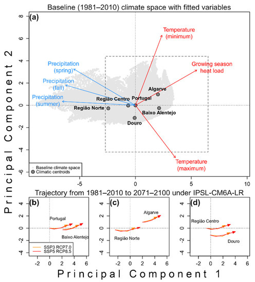
Figure 1.
Ordination plots of Portugal in climate space comprising six variables: precipitation in spring, summer, and fall, temperature extremes (min. and max.), and growing season heat load; (a) the arrows and light gray points represent fitted vectors of precipitation (blue) and heat (red) and the entire baseline climate space, respectively, while the filled circles represent regional centroids; (b–d) climatic trajectories under climate change following SSP3-7.0 (orange) and SSP5-8.5 (red).
In Tables S5 and S6, we provide the 25th, 50th, and 75th percentiles of climate variables computed for the baseline and future time periods across Portugal and for both SSP3-7.0 and SSP5-8.5 to complement Figure 1 and help the interpretation of the predictions. In short, these tables reveal a continuous increase in temperature (both TMIN and TMAX) coupled with a continuous decrease in overall precipitation (not considering winter precipitation). Compared with the baseline (1981–2100), the median temperature increased from 4.7 °C (TMIN) and 28.8 °C (TMAX) to 7.3 °C and 34.4 °C (SSP3-7.0), and 8.1 °C and 35.7 °C (SSP5-8.5) by 2071–2100. The precipitation decrease was found to be mostly driven by a decrease in spring, from 200 mm in 1981–2010 to 157 mm (SSP3-7.0) and 150 mm (SSP5-8.5) in 2071–2100 (Tables S5 and S6). We also provide the same climate variable percentiles for the focal areas (Norte, Douro, Centro, Baixo Alentejo, and Algarve) under both SSP3-7.0 (Tables S7, S9, S11, S13 and S15) and SSP5-8.5 (Tables S8, S10, S12, S14 and S16) but stop short of presenting and discussing these in detail for brevity.
The replicate models were mostly influenced (rounded to one decimal) by TMAX (17.5%), GSHS (14.3%), IRRI (13.3%), and PSummer (12.9%), and least affected by HLI (2.6%), PFall (3.2%), and SPH (5.0%). The mean contribution of HLI was comparatively low but stable (sd = 0.227) and remained above 2.0% across all replicate models. Moreover, PSpring (11.2%), TMIN (8.3%), Clay (6.5%), and Coarse (5.3%) also substantially contributed to the models.
Overall, mean evaluation metrics across all replicates suggested excellent model performance (AUCtrain = 0.932; AUCtest = 0.901; TSS = 0.638) and limited overfitting (AUCdif. = 0.032). Moreover, the replicate models performed in a consistent way, with the minimum AUCtrain, AUCtest, and TSS values being approximately equal to 0.929, 0.894, and 0.628, respectively. Similarly, the maximum AUCdif. value was equal to ~0.041. The TSS and AUCdif. cutoffs representing the 10th and 90th percentiles were approximately equal to 0.630 and 0.037, respectively, and led to the elimination of five replicate models. The resulting ensemble (computed as the median of the remaining 25 replicate models) was evaluated using the median of the retained replicate models’ thresholds and the TSS and achieved a score of ~0.640, which is comparable to an excellent AUC score of ~0.820.
The ensemble predictions of grapevine suitability, clipped to regions above the 10th percentile cutoff, for the baseline period (1981–2100) and both irrigation scenarios (with and without irrigation) are shown in Figure 2. Moreover, we provide Figure 2, Figure 3 and Figure 4, which contrast both irrigation scenarios and climate trajectories for the periods 2011–2040, 2041–2070, and 2071–2100. In addition, Table 1 and Table 2 summarize the expanse and mean suitability of regions predicted as suitable for viticulture, alongside changes relative to the baseline scenario with irrigation. All ensemble predictions are available in a repository (https://doi.org/10.6084/m9.figshare.21587229; created on 20 November 2022) to facilitate analysis of different regions and comparisons between studies.
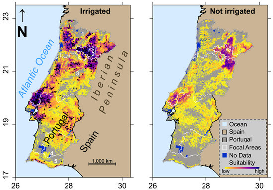
Figure 2.
Predictions (EPSG:3035) for the baseline period (1981–2010) with coordinates in hundreds of kilometers. Darker colors indicate higher suitability; suitability falls short of the 10th percentile threshold, and no data regions are shown in gray and dark blue, respectively. The outlines of the Douro wine region and the other focal areas are displayed in white. In the left panel, we also overlay a systematic subset of 500 out of 7002 presences (black triangles) to allow for a visual assessment of the prediction and numeric labels (1–5) to identify different regions: “1” Norte, “2” Douro wine region, “3” Centro, “4” Baixo Alentejo, and “5” Algarve. (Left) Actual proportions of area equipped for irrigation are used; (Right) the proportion of area equipped for irrigation is assumed zero across the study area. Geographic labels are added in the first panel for faster orientation.
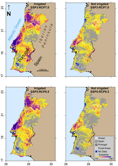
Figure 3.
Predictions (EPSG:3035) for the 2011–2040 period; the figure follows the style of Figure 2. (Left panels) with irrigation, (right panels) without irrigation, (top panels) SSP3-7.0 climate trajectory, (bottom) SSP5-8.5 climate trajectory.
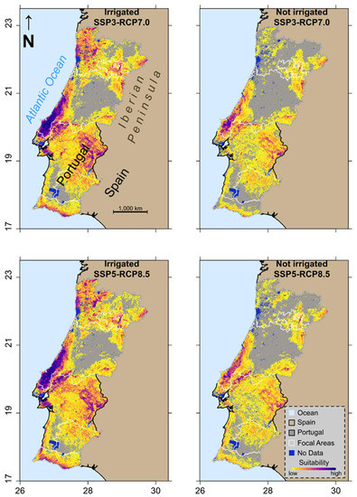
Figure 4.
Predictions (EPSG:3035) for the 2041–2070 period; the figure follows the style of Figure 2. (Left panels) with irrigation, (right panels) without irrigation, (top panels) SSP3-7.0 climate trajectory, (bottom) SSP5-8.5 climate trajectory.

Table 1.
Summary of the most extreme climate change scenario effects under continued irrigation on the suitable area relative to the baseline period (1981–2010) across Portugal and the five focal areas.
Table 2.
Summary of the most extreme climate change scenario effects without irrigation on suitable area relative to the baseline period (1981–2010) across Portugal and the five focal areas.
The baseline scenario with the actual irrigation data suggests widely suitable climates for viticulture across Portugal, with particularly large expanses of high suitability found across the north and west of Portugal (Figure 2 left panel). When considering the same baseline period but without irrigation (Figure 2 right panel), the predicted suitability appeared reduced, and high suitability was mostly confined to regions of limited extent in the northeast (e.g., Douro, Dão, and Bairrada) and the west (mostly around Lisbon in the center-west, e.g., Alenquer and Palmela). The future predictions for the three future periods, 2011–2040 (Figure 3), 2041–2070 (Figure 4), and 2071–2100 (Figure 5), differed both between climate trajectories (top vs. bottom panels) and irrigation scenarios (left vs. right panels) with no irrigation scenarios consistently causing greater apparent reductions in suitable area and suitability, while the distinction between SSP3-7.0 and SSP5-8.5 was less clear. Moreover, there appeared to be a trend of suitable regions shifting to and being associated with coastal areas.
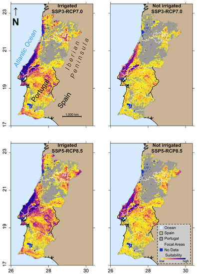
Figure 5.
Predictions (EPSG:3035) for the 2071–2100 period; the figure follows the style of Figure 2. (Left panels) with irrigation, (right panels) without irrigation, (top panels) SSP3-7.0 climate trajectory, (bottom) SSP5-8.5 climate trajectory.
Overall, suitable regions look poised to contract under climate change, although initially stable regarding area and with limited recovery in the 2041–2070 and 2071–2100 periods (depending on the region), and exhibit reduced suitability for viticulture (Figure 2, Figure 3 and Figure 4). Moreover, suitable viticulture regions appeared to generally shift toward the coastal regions. Contractions appeared most severe in the northern half of Portugal, including in the Douro wine region and adjacent regions (e.g., Dão and Bairrada), and least severe in the south and west of Portugal, which appeared to profit from climate change. In western Portugal, suitable regions were predicted to expand and shift into a coastal band shape stretching approximately from Lisbon (38°43′ N, 9°10′ W) to Aveiro (40°38′ N, 8°39′ W). Finally, the influence of the different climate trajectories appeared to show overall lowered suitability under SSP5-8.5 relative to SSP3-7.0 but not necessarily a reduction in suitable area to a similar degree and strong regional differences (Figure 2, Figure 3 and Figure 4).
Table 1 and Table 2 and summaries of Tables S1–S4 which detail the estimated expanses of the suitable area and mean suitability within the former across Portugal and within the five focal areas for perpetuated (Table S1 and Table S3) and no irrigation (Table S2 and Table S4) under climate trajectories SSP3-7.0 (Table S1 and Table S2) and SSP5-8.5 (Table S2 and Table S3), respectively.
The largest loss of suitable area across Portugal occurred in the 2041–2070 period under SSP3-7.0; without irrigation, however, an almost fourfold larger loss is expected for the 2011–2040 period under SSP5-8.5. The largest predicted gains occurred in the Algarve and Baixo Alentejo, where the suitable areas could more than triple and almost double under SSP5-8.5—provided that irrigation patterns do not change (Table 1). Without irrigation, however, each of these two areas would have experienced almost complete losses of suitable area in the baseline period (Table 2). Large losses (>40%) are also expected for the Douro wine region, Norte, and Centro—and even with irrigation.
Finally, our coarse extrapolation suggests that wine production would decrease by approximately 21% or 1.5 million hectoliters (SSP3-7.0 with irrigation), 69% or 5.0 million hectoliters (SSP3-7.0 without irrigation), and 48% or 3.5 million hectoliters (SSP5-8.5 without irrigation), but would—overall—remain stable (plus ~0.7% or ~51 thousand hectoliters) under SSP5-8.5 with irrigation when compared with the 1995 wine production in Portugal of ~7.3 million hectoliters according to the OIV database (https://www.oiv.int/en/statistiques/recherche; [88]; accessed on 15 August 2022).
4. Discussion
In this study, we have analyzed the climatic shifts in Portugal and modeled regional grapevine suitability across the study area and in five focal areas to estimate national and regional climate change effects on the suitable area and mean suitability of grapevine cultivation. The models were mostly driven by temperature (TMAX and GSHS) and water availability (IRRI and PSummer). Given the expectations of succinctly rising median TMAX (>5 °C) and declining precipitation in spring (>20%) and overall (Tables S5 and S6), with little reason to expect betterment of global climate trends in the near future [67], it is not surprising that our predictions suggest major losses across Portugal and in most focal areas, particularly when assuming a halt to irrigation (Table 1, Table 2 and Tables S1–S4). This is, since plants face a trade-off between photosynthetic activity and water conservation as temperatures rise with increasing CO2 levels, even if water-use efficiency would increase [89]. Consequently, the trends toward drier and warmer climates in Portugal would promote water conservation and, thus, reduced photosynthetic activity. For plants in drier regions, it is generally expected that elevated CO2 would contribute to increasing greenness and leaf area; however, the increased sensitivity to water availability would make the plants more susceptible to droughts [90]. Specifically for grapevine, however, elevated CO2 was shown to accelerate berry ripening while reducing production [91] and contribute to increased net photosynthetic rate, water-use efficiency, and grapevine yield under current temperature regimes, without significant stomatal conductance responses under drought conditions [92]. According to the same study, the latter could be attributed to the experimental drought conditions not being severe enough to trigger such a response [92], and another study observed such stomatal acclimation responses and reduced photosynthetic capacity under elevated CO2, at least 20 days after treatments were imposed—even when temperature and water availability were not modified and more so if this was the case [93]. This makes the expected tendencies toward increasing drought frequency and severity in the region troubling [21].
Consistently high evaluation scores on test data and relatively low overfitting suggest that our results are both robust and suitable for deriving future predictions [81,94]. However, since we did not differentiate between varieties, the estimated niche of grapevine would represent the union of all individual varietal niches, which may differ in their requirements for water, growing degree days [33], and other factors. Such intraspecific variability is known in grapevine cultivars, for example, in terms of growing degree requirements [33], and has also been reported for other taxa, such as grasses [87]. Therefore, the effect of climate change in individual wine regions, which typically cultivate one or a few dominant varieties that are well adapted to the local conditions, might also be underestimated. Since human-facilitated dispersal, that is, the planting of different, better-adapted varieties [33], is highly likely, however, we may also overestimate on-the-ground climate change impacts due to the buffering effect of intraspecific variability [95]. In addition, management responses including shading [96], especially with novel photo-selective materials [97], adjusted pruning times [98], and improved irrigation [47,99], for example, carbonated irrigation [100], and other emerging technologies would reduce the predicted impacts. Our results, thus, have to be seen as a prediction of what could happen when no changes are made to current practice (other than irrigation, for which we provide an alternative scenario), which in our opinion, represents the best information to identify regions where management responses to climate change are required. Moreover, our no irrigation scenario shows the potential ramifications of failing to maintain (let alone expand) current irrigation practices under a drying climate. Since lowered precipitation (Tables S5 and S6) would lead to reduced water tables, stream flows, and reservoir storage levels, less water would be available for agriculture. As we have demonstrated, this could cause dramatic consequences for the cultivation of not just grapevines but also similarly drought-tolerant crops, such as olives (Olea europaea), and generally (even more so) for other (less drought tolerant) crops grown in the region, including rice, which typically requires inundation.
Our results are not in line with the findings of Gouveia and colleagues [37], who predicted favorable consequences of climate change for the Douro wine region, but largely agree with those of Blanco-Ward and colleagues [39] about future climate change effects on wine production; overall, we suggest a negative outcome with substantial net losses of suitable area, particularly in the 2041–2070 and 2011–2040 periods and, regarding specific focal areas, in the Região Norte, the Douro wine region, and the Região Centro (Table 1, Table 2 and Tables S1–S4, Figure 2, Figure 3 and Figure 4). While potential recoveries are expected in some regions, they might not be realistic, considering that grapevines bear no fruit for several years after planting and might not reach peak product until after a decade [7]. A similar trajectory under climate change, that is, a large decline of suitable area by 2041–2070 with a subsequent partial recovery, has been reported for southern Italy due to the combined effects of increasing temperature and prolonged dry spells [16].
Our results are concerning, given the economic and cultural relevance of grapevine cultivation and winemaking in Portugal and—specifically—the Douro wine region [31]. Considering that the predicted losses were most and least severe in the north and south of Portugal, respectively—in fact, regions in the south might greatly, albeit most likely in theory only, profit from climate change given continuing irrigation (Table 1 and Table 2; Figure 2, Figure 3 and Figure 4)—the predicted pattern suggests a shift from northern to southern viticulture areas. This trend contrasts large-scale poleward boundary shifts of viticulture [27,101] and suggests that the grapevine is locally and regionally subject to complex interactions between individual aspects of terroir [14]. In addition, we observed a clear tendency of higher suitability shifting toward the coast (Figure 2, Figure 3 and Figure 4), which could partly be explained by the mediating effect of the Atlantic Ocean on extreme temperatures. In the Algarve, which resembles a band along the southern coast, for example, the median TMAX is predicted to increase only by 2.9 °C (SSP3-7.0) to 3.7 °C (SSP5-8.5) by 2071–2100 (Tables S15 and S16), whereas the same increase would be equal to 5.6 °C (SSP3-7.0) to 6.9 °C (SSP5-8.5) across continental Portugal (Tables S5 and S6). Finally, increasing temperatures early in the season could affect the grapevine phenology and result in hastened berry maturation and potentially reduce production [91].
Moreover, assuming that wine production volume is dependent on the product of suitable area and mean suitability, our results suggested mostly major reductions in production volume relative to the baseline period of roughly 21% to 69% by 2071–2100, except for the SSP5-8.5 scenario with irrigation, which caused a marginal increase (0.7%). Our extrapolation is, of course, rough. While suitability is known to be generally positively correlated with abundance [102] and thence biomass, our assumptions are unlikely to withstand rigorous tests, in particular due to negligence of many factors (including market mechanics and mitigation measures) and the nonlinearity of the suitability–abundance relationship [103]. Nevertheless, our extrapolation helps to appreciate the potential magnitude of a crisis that is at least partly preventable.
Surprisingly, suitability for grapevine or viticulture decreased in the north, most severely in the Douro wine region and the Região Norte, and—less extreme—in the Região Centro, but not in the south, where suitable area was actually found to potentially increase, especially in the Algarve (Table 1 and Table 2). This represents an inversion of the typical climate change impacts since Portugal, together with Spain, Italy, and Greece, sits at or close to the northern hemisphere’s southern limit of grape cultivation and winemaking. Therefore, an overall northward shift would have been expected given the geographic position of Portugal in the northern hemisphere, in line with large-scale responses to climate change of viticulture [27,28] and many species [104]. For example, wine is now grown in northern countries, such as Latvia, Denmark, Sweden, and even Finland and Norway [27,101,105]. Similarly, global “breadbaskets” are likely required to shift poleward to avoid severe yield shortages [106]; however, crop pests, such as locusts or moths, are expected to expand their ranges poleward [24,25] too. Moreover, losses were exacerbated, and potential increases in suitable area, that is, in the Algarve and Baixo Alentejo, were turned into losses when irrigation was assumed to stop (Table 2). Therefore, our study highlights the complexities of viticulture responses to climate change when considering the potential effects of climate variable interactions, changing agricultural practices, and potential mitigation.
While the viticulture outlook for many regions in Portugal is bleak, well-established and emerging management adaptation and mitigation strategies are available. Potential pathways to ameliorate or mitigate climate change effects on wine quantity and quality [28] include adjusted pruning times, improved irrigation [100], water nebulization to limit peak heat stress [107], selection of more suitable varieties [7,33], and shading or kaolin (Al4Si4O10(OH)8) coating against radiation and heat [33,96,97,98,99,107,108]. Depending on the exact makeup of shading, however, it might reduce plant biomass by affecting the carbon balance, as shown for apple [109], while installation costs (or lacking water resources) might prevent the widespread use of nebulization [107], or even irrigation. Kaolin coating, similarly, can be effective against the impacts of radiation and heat and thus can maintain yields but might slightly decrease sugar content in berries [107]. In addition, new varieties can be bred that are more resilient to climate change (e.g., tolerant to higher temperatures and more frequent droughts, or with longer maturation periods), particularly when harnessing genetic methods [110,111] that can also improve pathogen resistance [112]. Moreover, plant-growth-promoting microbes (PGPMs) could help to further improve the tolerance of grapevines to climatic stress or disease [113,114,115], yet more research will be required, including on the biosafety of such approaches. As a last resort, vineyards could be moved to cooler sites, for example, on north-facing slopes or higher elevations [39], although such climate change adaptation strategies would also come with their own challenges, such stressful levels of UV-B radiation at higher elevation [116], and, thus, require additional mitigation. Moreover, planting new varieties or establishing new vineyards at cooler sites, or to reclaim regions lost before due to climate change, also takes time since grapevines do not produce crop for several years after planting and may reach peak production after a decade or later [7].
Altogether, these limitations and complications suggest the need for substantial investments for adaptation or, in some regions, to facilitate transition to other, more favorable crops or land uses. Finally, given the critical importance of irrigation, adaptation strategies aiming to preserve or provide additional water resources, for example, by partly covering reservoirs, canals, aquaculture ponds, and other water bodies with floating solar panels [117,118,119] or by desalination and reusing wastewater [120,121], would likely also be required alongside a range of policy changes regulating water use [122] and encouraging collective action [123] for resilient food production systems under an increasingly drier climate, which might cause competition [124] for increasingly scarce irrigation water resources.
5. Conclusions
Climate change has the potential to expand viticulture poleward by elevating average temperatures. In most traditional viticulture regions, however, this potentially positive effect of rising temperature is offset by increased water requirements (i.e., irrigation), while droughts tend to become more frequent and longer. In this study, we found that climate change would have overall negative consequences for viticulture in Portugal, and potentially devastating consequences for the Região Norte, the Douro wine region, and the Região Centro (except its westernmost coastal areas), unless intensive mitigation strategies are pursued, particularly when irrigation becomes limited or impossible. While increased and improved irrigation might mitigate some of these impacts, it remains questionable whether freshwater sources for irrigation are readily available under an increasingly drier climate. In summary, climate change will likely have broad and mostly negative effects on Portugal’s viticulture, while hypothetically presenting opportunities (if water is available) in some regions, such as the Algarve, and will make necessary a range of adaptive mitigation strategies, including cultivar selection and breeding, inoculation with PGPMs, improved irrigation, and other techniques, such as shading. However, PGPMs for grapevine are still in their infancy, and water for irrigation might be lacking in the near future, making regional transitions to even more drought-tolerant crops or agricultural systems potentially inevitable if traditional mitigation measures fall short of mitigating worsening climate change impacts.
Supplementary Materials
The following supporting information can be downloaded at: https://www.mdpi.com/article/10.3390/environments10010005/s1, Table S1: Expanses of suitable area and mean suitability in Portugal and five focal areas for the baseline period and three future predictions under SSP3-7.0 with irrigation remaining unchanged; Table S2: Expanses of suitable area and mean suitability in Portugal and five focal areas for the baseline period and three future predictions under SSP3-7.0 with irrigation being stopped; Table S3: Expanses of suitable area and mean suitability in Portugal and five focal areas for the baseline period and three future predictions under SSP5-8.5 with irrigation remaining unchanged; Table S4: Expanses of suitable area and mean suitability in Portugal and five focal areas for the baseline period and three future predictions under SSP5-8.5 with irrigation being stopped; Table S5: 25th, 50th, and 75th percentiles across Portugal of the six climate variables, growing season (10 °C) heat sum, minimum and maximum temperature (TMIN and TMAX), GSHS, and the precipitation in spring, summer, and fall (PSpring, PSummer, PFall), for the baseline (1981–2010) and three future periods spanning from 2011 to 2100 under SSP3-7.0; Table S6: 25th, 50th, and 75th percentiles across Portugal of the six climate variables, growing season (10 °C) heat sum, minimum and maximum temperature (TMIN and TMAX), and the precipitation in spring, summer, and fall (PSpring, PSummer, PFall), for the baseline (1981–2010) and three future periods spanning from 2011 to 2100 under SSP5-8.5; Table S7: 25th, 50th, and 75th percentiles in Região Norte of the six climate variables, growing season (10 °C) heat sum, minimum and maximum temperature (TMIN and TMAX), and the precipitation in spring, summer, and fall (PSpring, PSummer, PFall), for the baseline (1981–2010) and three future periods spanning from 2011 to 2100 under SSP3-7.0; Table S8: 25th, 50th, and 75th percentiles in Região Norte of the six climate variables, growing season (10 °C) heat sum, minimum and maximum temperature (TMIN and TMAX), and the precipitation in spring, summer, and fall (PSpring, PSummer, PFall), for the baseline (1981–2010) and three future periods spanning from 2011 to 2100 under SSP5-8.5; Table S9: 25th, 50th, and 75th percentiles in the Douro wine region of the six climate variables, growing season (10 °C) heat sum, minimum and maximum temperature (TMIN and TMAX), and the precipitation in spring, summer, and fall (PSpring, PSummer, PFall), for the baseline (1981–2010) and three future periods spanning from 2011 to 2100 under SSP3-7.0; Table S10: 25th, 50th, and 75th percentiles in the Douro wine region of the six climate variables, growing season (10 °C) heat sum, minimum and maximum temperature (TMIN and TMAX), and the precipitation in spring, summer, and fall (PSpring, PSummer, PFall), for the baseline (1981–2010) and three future periods spanning from 2011 to 2100 under SSP5-8.5; Table S11: 25th, 50th, and 75th percentiles in Região Centro of the six climate variables, growing season (10 °C) heat sum, minimum and maximum temperature (TMIN and TMAX), and the precipitation in spring, summer, and fall (PSpring, PSummer, PFall), for the baseline (1981–2010) and three future periods spanning from 2011 to 2100 under SSP3-7.0; Table S12: 25th, 50th, and 75th percentiles in Região Centro of the six climate variables, growing season (10 °C) heat sum, minimum and maximum temperature (TMIN and TMAX), and the precipitation in spring, summer, and fall (PSpring, PSummer, PFall), for the baseline (1981–2010) and three future periods spanning from 2011 to 2100 under SSP5-8.5; Table S13: 25th, 50th, and 75th percentiles in Baixo Alentejo of the six climate variables, growing season (10 °C) heat sum, minimum and maximum temperature (TMIN and TMAX), and the precipitation in spring, summer, and fall (PSpring, PSummer, PFall), for the baseline (1981–2010) and three future periods spanning from 2011 to 2100 under SSP3-7.0; Table S14: 25th, 50th, and 75th percentiles in Baixo Alentejo of the six climate variables, growing season (10 °C) heat sum, minimum and maximum temperature (TMIN and TMAX), and the precipitation in spring, summer, and fall (PSpring, PSummer, PFall), for the baseline (1981–2010) and three future periods spanning from 2011 to 2100 under SSP5-8.5; Table S15: 25th, 50th, and 75th percentiles in the Algarve of the six climate variables, growing season (10 °C) heat sum, minimum and maximum temperature (TMIN and TMAX), and the precipitation in spring, summer, and fall (PSpring, PSummer, PFall), for the baseline (1981–2010) and three future periods spanning from 2011 to 2100 under SSP3-7.0; Table S16: 25th, 50th, and 75th percentiles in the Algarve of the six climate variables, growing season (10 °C) heat sum, minimum and maximum temperature (TMIN and TMAX), and the precipitation in spring, summer, and fall (PSpring, PSummer, PFall), for the baseline (1981–2010) and three future periods spanning from 2011 to 2100 under SSP5-8.5.
Author Contributions
Conceptualization, R.F.W. and Y.-P.L.; methodology, R.F.W.; software, R.F.W.; validation, Y.-P.L. and A.A.; formal analysis, R.F.W.; data curation, R.F.W.; writing—original draft preparation, R.F.W.; writing—review and editing, Y.-P.L. and A.A.; visualization, R.F.W. and A.A.; supervision, Y.-P.L. All authors have read and agreed to the published version of the manuscript.
Funding
This research received no external funding.
Data Availability Statement
This research was based entirely on openly available datasets. Results and code are available upon reasonable request from the authors.
Acknowledgments
We are grateful to all scholars having provided comments on earlier versions of this manuscript.
Conflicts of Interest
The authors declare no conflict of interest.
References
- Research And Markets Wine—Global Market Trajectory & Analytics. Available online: https://www.researchandmarkets.com/reports/338680/ (accessed on 1 August 2022).
- McGovern, P.; Jalabadze, M.; Batiuk, S.; Callahan, M.P.; Smith, K.E.; Hall, G.R.; Kvavadze, E.; Maghradze, D.; Rusishvili, N.; Bouby, L.; et al. Early Neolithic wine of Georgia in the South Caucasus. Proc. Natl. Acad. Sci. USA 2017, 114, E10309–E10318. [Google Scholar] [CrossRef] [PubMed]
- Vavilov, N.I. From Bulletin of Applied Botany and Plant Breeding, 16, 2, 1926, Leningrad. Bull. Appl. Bot. Plant Breed. 1926, 16. [Google Scholar]
- Vouillamoz, J.F.; McGovern, P.E.; Ergul, A.; Söylemezoğlu, G.; Tevzadze, G.; Meredith, C.P.; Grando, M.S. Genetic characterization and relationships of traditional grape cultivars from Transcaucasia and Anatolia. Plant Genet. Resour. 2006, 4, 144–158. [Google Scholar] [CrossRef]
- Myles, S.; Boyko, A.R.; Owens, C.L.; Brown, P.J.; Grassi, F.; Aradhya, M.K.; Prins, B.; Reynolds, A.; Chia, J.M.; Ware, D.; et al. Genetic structure and domestication history of the grape. Proc. Natl. Acad. Sci. USA. 2011, 108, 3530–3535. [Google Scholar] [CrossRef] [PubMed]
- Chloupek, O.; Hrstkova, P.; Schweigert, P. Yield and its stability, crop diversity, adaptability and response to climate change, weather and fertilisation over 75 years in the Czech Republic in comparison to some European countries. F. Crop. Res. 2004, 85, 167–190. [Google Scholar] [CrossRef]
- Goode, J. Viticulture: Fruity with a hint of drought. Nature 2012, 492, 351–352. [Google Scholar] [CrossRef] [PubMed][Green Version]
- Yamane, T.; Seok, T.J.; Goto-Yamamoto, N.; Koshita, Y.; Kobayashi, S. Effects of temperature on anthocyanin biosynthesis in grape berry skins. Am. J. Enol. Vitic. 2006, 57, 54–59. [Google Scholar] [CrossRef]
- Mori, K.; Goto-Yamamoto, N.; Kitayama, M.; Hashizume, K. Loss of anthocyanins in red-wine grape under high temperature. J. Exp. Bot. 2007, 58, 1935–1945. [Google Scholar] [CrossRef]
- Downey, M.O.; Dokoozlian, N.K.; Krstic, M.P. Cultural practice and environmental impacts on the flavonoid composition of grapes and wine: A review of recent research. Am. J. Enol. Vitic. 2006, 57, 257–268. [Google Scholar] [CrossRef]
- Mira de Orduña, R. Climate change associated effects on grape and wine quality and production. Food Res. Int. 2010, 43, 1844–1855. [Google Scholar] [CrossRef]
- Teslić, N.; Zinzani, G.; Parpinello, G.P.; Versari, A. Climate change trends, grape production, and potential alcohol concentration in wine from the “Romagna Sangiovese” appellation area (Italy). Theor. Appl. Climatol. 2018, 131, 793–803. [Google Scholar] [CrossRef]
- Venios, X.; Korkas, E.; Nisiotou, A.; Banilas, G. Grapevine responses to heat stress and global warming. Plants 2020, 9, 1754. [Google Scholar] [CrossRef] [PubMed]
- Gladstones, J. Wine, Terroir and Climate Change; Wakefield Press: Adelaide, Australia, 2011; ISBN 9781862549241. [Google Scholar]
- Fraga, H.; Malheiro, A.C.; Moutinho-Pereira, J.; Santos, J.A. Climate factors driving wine production in the Portuguese Minho region. Agric. For. Meteorol. 2014, 185, 26–36. [Google Scholar] [CrossRef]
- Bonfante, A.; Monaco, E.; Langella, G.; Mercogliano, P.; Bucchignani, E.; Manna, P.; Terribile, F. A dynamic viticultural zoning to explore the resilience of terroir concept under climate change. Sci. Total Environ. 2018, 624, 294–308. [Google Scholar] [CrossRef] [PubMed]
- Jones, G.V.; Reid, R.; Vilks, A. Climate, Grapes, and Wine: Structure and Suitability in a Variable and Changing Climate BT—The Geography of Wine: Regions, Terroir and Techniques; Dougherty, P.H., Ed.; Springer Netherlands: Dordrecht, The Netherlands, 2012; pp. 109–133. ISBN 978-94-007-0464-0. [Google Scholar]
- Ramos, M.C.; Jones, G.V.; Martínez-Casasnovas, J.A. Structure and trends in climate parameters affecting winegrape production in northeast Spain. Clim. Res. 2008, 38, 1–15. [Google Scholar] [CrossRef]
- Spinoni, J.; Vogt, J.V.; Naumann, G.; Barbosa, P.; Dosio, A. Will drought events become more frequent and severe in Europe? Int. J. Climatol. 2018, 38, 1718–1736. [Google Scholar] [CrossRef]
- Büntgen, U.; Urban, O.; Krusic, P.J.; Rybníček, M.; Kolář, T.; Kyncl, T.; Ač, A.; Koňasová, E.; Čáslavský, J.; Esper, J.; et al. Recent European drought extremes beyond Common Era background variability. Nat. Geosci. 2021, 14, 190–196. [Google Scholar] [CrossRef]
- García-Valdecasas Ojeda, M.; Gámiz-Fortis, S.R.; Romero-Jiménez, E.; Rosa-Cánovas, J.J.; Yeste, P.; Castro-Díez, Y.; Esteban-Parra, M.J. Projected changes in the Iberian Peninsula drought characteristics. Sci. Total Environ. 2021, 757, 143702. [Google Scholar] [CrossRef]
- Rojas, R.; Feyen, L.; Watkiss, P. Climate change and river floods in the European Union: Socio-economic consequences and the costs and benefits of adaptation. Glob. Environ. Chang. 2013, 23, 1737–1751. [Google Scholar] [CrossRef]
- Alfieri, L.; Burek, P.; Feyen, L.; Forzieri, G. Global warming increases the frequency of river floods in Europe. Hydrol. Earth Syst. Sci. 2015, 19, 2247–2260. [Google Scholar] [CrossRef]
- Peng, W.; Ma, N.L.; Zhang, D.; Zhou, Q.; Yue, X.; Khoo, S.C.; Yang, H.; Guan, R.; Chen, H.; Zhang, X.; et al. A review of historical and recent locust outbreaks: Links to global warming, food security and mitigation strategies. Environ. Res. 2020, 191, 110046. [Google Scholar] [CrossRef] [PubMed]
- Svobodová, E.; Trnka, M.; Dubrovský, M.; Semerádová, D.; Eitzinger, J.; Štěpánek, P.; Žalud, Z. Determination of areas with the most significant shift in persistence of pests in Europe under climate change. Pest Manag. Sci. 2014, 70, 708–715. [Google Scholar] [CrossRef] [PubMed]
- Hannah, L.; Roehrdanz, P.R.; Ikegami, M.; Shepard, A.V.; Shaw, M.R.; Tabor, G.; Zhi, L.; Marquet, P.A.; Hijmans, R.J. Climate change, wine, and conservation. Proc. Natl. Acad. Sci. USA 2013, 110, 6907–6912. [Google Scholar] [CrossRef] [PubMed]
- Schultz, H.R.; Jones, G.V. Climate Induced Historic and Future Changes in Viticulture. J. Wine Res. 2010, 21, 137–145. [Google Scholar] [CrossRef]
- Jones, G.V.; White, M.A.; Cooper, O.R.; Storchmann, K. Climate Change and Global Wine Quality. Clim. Change 2005, 73, 319–343. [Google Scholar] [CrossRef]
- Mora, C.; Vieira, G. The Climate of Portugal. In World Geomorphological Landscapes; Vieira, G., Zêzere, J.L., Mora, C., Eds.; Springer International Publishing: Cham, Switzerland, 2020; pp. 33–46. ISBN 978-3-319-03641-0. [Google Scholar]
- Lenoir, J.; Hattab, T.; Pierre, G. Climatic microrefugia under anthropogenic climate change: Implications for species redistribution. Ecography 2017, 40, 253–266. [Google Scholar] [CrossRef]
- UNESCO. Alto Douro Wine Region. Available online: https://whc.unesco.org/en/list/1046/ (accessed on 1 August 2022).
- Kottek, M.; Grieser, J.; Beck, C.; Rudolf, B.; Rubel, F. World map of the Köppen-Geiger climate classification updated. Meteorol. Zeitschrift 2006, 15, 259–263. [Google Scholar] [CrossRef]
- Fraga, H.; Santos, J.A.; Malheiro, A.C.; Oliveira, A.A.; Moutinho-Pereira, J.; Jones, G.V. Climatic suitability of Portuguese grapevine varieties and climate change adaptation. Int. J. Climatol. 2016, 36, 1–12. [Google Scholar] [CrossRef]
- Statista Wine: Portugal. Available online: https://www.statista.com/outlook/cmo/alcoholic-drinks/wine/portugal (accessed on 1 August 2022).
- Jiménez-Ballesta, R.; Bravo, S.; Amorós, J.A.; Pérez-de-los-Reyes, C.; García-Pradas, J.; Sánchez, M.; García-Navarro, F.J. An Environmental Approach to Understanding the Expansion of Future Vineyards: Case Study of Soil Developed on Alluvial Sediments. Environments 2021, 8, 96. [Google Scholar] [CrossRef]
- Aguirre-Liguori, J.A.; Morales-Cruz, A.; Gaut, B.S. Evaluating the persistence and utility of five wild Vitis species in the context of climate change. Mol. Ecol. 2022, 31, 6457–6472. [Google Scholar] [CrossRef]
- Gouveia, C.; Liberato, M.; DaCamara, C.; Trigo, R.; Ramos, A. Modelling past and future wine production in the Portuguese Douro Valley. Clim. Res. 2011, 48, 349–362. [Google Scholar] [CrossRef]
- Hristov, J. An Exploratory Analysis of the Impact of Climate Change on Macedonian Agriculture. Environments 2017, 5, 3. [Google Scholar] [CrossRef]
- Blanco-Ward, D.; Monteiro, A.; Lopes, M.; Borrego, C.; Silveira, C.; Viceto, C.; Rocha, A.; Ribeiro, A.; Andrade, J.; Feliciano, M.; et al. Climate change impact on a wine-producing region using a dynamical downscaling approach: Climate parameters, bioclimatic indices and extreme indices. Int. J. Climatol. 2019, 39, 5741–5760. [Google Scholar] [CrossRef]
- Bindi, M.; Fibbi, L.; Gozzini, B.; Orlandini, S.; Miglietta, F. Modelling the impact of future climate scenarios on yield and yield variability of grapevine. Clim. Res. 1996, 7, 213–224. [Google Scholar] [CrossRef]
- Bai, H.; Sun, Z.; Yao, X.; Kong, J.; Wang, Y.; Zhang, X.; Chen, W.; Fan, P.; Li, S.; Liang, Z.; et al. Viticultural Suitability Analysis Based on Multi-Source Data Highlights Climate-Change-Induced Decrease in Potential Suitable Areas: A Case Analysis in Ningxia, China. Remote Sens. 2022, 14, 3717. [Google Scholar] [CrossRef]
- Guisan, A.; Zimmermann, N.E. Predictive habitat distribution models in ecology. Ecol. Modell. 2000, 135, 147–186. [Google Scholar] [CrossRef]
- Valavi, R.; Guillera-Arroita, G.; Lahoz-Monfort, J.J.; Elith, J. Predictive performance of presence-only species distribution models: A benchmark study with reproducible code. Ecol. Monogr. 2022, 92, e1486. [Google Scholar] [CrossRef]
- Elith, J.; Phillips, S.J.; Hastie, T.; Dudík, M.; Chee, Y.E.; Yates, C.J. A statistical explanation of MaxEnt for ecologists. Divers. Distrib. 2011, 17, 43–57. [Google Scholar] [CrossRef]
- Peterson, A.T. Predicting Species’ Geographic Distributions Based on Ecological Niche Modeling. Condor 2001, 103, 599–605. [Google Scholar] [CrossRef]
- Rodrigues, P.; Pedroso, V.; Reis, S.; Yang, C.; Santos, J.A. Climate change impacts on phenology and ripening of cv. Touriga Nacional in the Dão wine region, Portugal. Int. J. Climatol. 2022, 42, 7117–7132. [Google Scholar] [CrossRef]
- Fraga, H.; García de Cortázar Atauri, I.; Santos, J.A. Viticultural irrigation demands under climate change scenarios in Portugal. Agric. Water Manag. 2018, 196, 66–74. [Google Scholar] [CrossRef]
- Martins, J.; Fraga, H.; Fonseca, A.; Santos, J.A. Climate Projections for Precipitation and Temperature Indicators in the Douro Wine Region: The Importance of Bias Correction. Agronomy 2021, 11, 990. [Google Scholar] [CrossRef]
- Ansari, A.; Lin, Y.-P.; Lur, H.-S. Evaluating and Adapting Climate Change Impacts on Rice Production in Indonesia: A Case Study of the Keduang Subwatershed, Central Java. Environments 2021, 8, 117. [Google Scholar] [CrossRef]
- Ngoy, K.I.; Shebitz, D. Potential impacts of climate change on areas suitable to grow some key crops in New Jersey, USA. Environments 2020, 7, 76. [Google Scholar] [CrossRef]
- Kourat, T.; Smadhi, D.; Madani, A. Modeling the Impact of Future Climate Change Impacts on Rainfed Durum Wheat Production in Algeria. Climate 2022, 10, 50. [Google Scholar] [CrossRef]
- GBIF Occurrence Download. Available online: https://www.gbif.org/occurrence/download/0422779-210914110416597 (accessed on 15 August 2022).
- Iturbide, M.; Bedia, J.; Herrera, S.; del Hierro, O.; Pinto, M.; Gutiérrez, J.M. A framework for species distribution modelling with improved pseudo-absence generation. Ecol. Modell. 2015, 312, 166–174. [Google Scholar] [CrossRef]
- Evans, J.S. spatialEco 2020; R Foundation for Statistical Computing: Vienna, Austria, 2020. [Google Scholar]
- Brun, P.; Zimmermann, N.E.; Hari, C.; Pellissier, L.; Karger, D.N. CHELSA-BIOCLIM+ A novel set of global climate-related predictors at kilometre-resolution. EnviDat. 2022. [Google Scholar] [CrossRef]
- Brun, P.; Zimmermann, N.E.; Hari, C.; Pellissier, L.; Karger, D.N. Global climate-related predictors at kilometre resolution for the past and future. Earth Syst. Sci. Data Discuss. 2022, 14, 5573–5603. [Google Scholar] [CrossRef]
- Karger, D.N.; Conrad, O.; Böhner, J.; Kawohl, T.; Kreft, H.; Soria-Auza, R.W.; Zimmermann, N.E.; Linder, H.P.; Kessler, M. Climatologies at high resolution for the earth’s land surface areas. Sci. Data 2017, 4, 170122. [Google Scholar] [CrossRef]
- Bobrowski, M.; Schickhoff, U. Why input matters: Selection of climate data sets for modelling the potential distribution of a treeline species in the Himalayan region. Ecol. Modell. 2017, 359, 92–102. [Google Scholar] [CrossRef]
- Ballabio, C.; Panagos, P.; Monatanarella, L. Mapping topsoil physical properties at European scale using the LUCAS database. Geoderma 2016, 261, 110–123. [Google Scholar] [CrossRef]
- Panagos, P.; Van Liedekerke, M.; Jones, A.; Montanarella, L. European Soil Data Centre: Response to European policy support and public data requirements. Land Use Policy 2012, 29, 329–338. [Google Scholar] [CrossRef]
- Hengl, T.; De Jesus, J.M.; Heuvelink, G.B.M.; Gonzalez, M.R.; Kilibarda, M.; Blagotić, A.; Shangguan, W.; Wright, M.N.; Geng, X.; Bauer-Marschallinger, B.; et al. SoilGrids250m: Global gridded soil information based on machine learning. PLoS ONE 2017, 12, e0169748. [Google Scholar] [CrossRef] [PubMed]
- McCune, B.; Keon, D. Equations for potential annual direct incident radiation and heat load. J. Veg. Sci. 2002, 13, 603–606. [Google Scholar] [CrossRef]
- McCune, B. Improved estimates of incident radiation and heat load using non- parametric regression against topographic variables. J. Veg. Sci. 2007, 18, 751–754. [Google Scholar] [CrossRef]
- Siebert, S.; Henrich, V.; Frenken, K.; Burke, J. Update of the Digital Global Map of Irrigation Areas to Version 5; Food and Agriculture Organization of the United Nations: Rome, Italy, 2013; Available online: https://www.researchgate.net/publication/264556183 (accessed on 1 August 2022).
- Boucher, O.; Servonnat, J.; Albright, A.L.; Aumont, O.; Balkanski, Y.; Bastrikov, V.; Bekki, S.; Bonnet, R.; Bony, S.; Bopp, L.; et al. Presentation and Evaluation of the IPSL-CM6A-LR Climate Model. J. Adv. Model. Earth Syst. 2020, 12, e2019MS002010. [Google Scholar] [CrossRef]
- Bonnet, R.; Boucher, O.; Deshayes, J.; Gastineau, G.; Hourdin, F.; Mignot, J.; Servonnat, J.; Swingedouw, D. Presentation and Evaluation of the IPSL-CM6A-LR Ensemble of Extended Historical Simulations. J. Adv. Model. Earth Syst. 2021, 13, e2021MS002565. [Google Scholar] [CrossRef]
- Horton, R. Offline: The fairy tale of Paris. Lancet 2022, 399, 2002. [Google Scholar] [CrossRef]
- O’Neill, B.C.; Kriegler, E.; Ebi, K.L.; Kemp-Benedict, E.; Riahi, K.; Rothman, D.S.; van Ruijven, B.J.; van Vuuren, D.P.; Birkmann, J.; Kok, K.; et al. The roads ahead: Narratives for shared socioeconomic pathways describing world futures in the 21st century. Glob. Environ. Chang. 2017, 42, 169–180. [Google Scholar] [CrossRef]
- Wunderlich, R.F.; Mukhtar, H.; Lin, Y.P. Comprehensively evaluating the performance of species distribution models across clades and resolutions: Choosing the right tool for the job. Landsc. Ecol. 2022, 37, 2045–2063. [Google Scholar] [CrossRef]
- Norberg, A.; Abrego, N.; Blanchet, F.G.; Adler, F.R.; Anderson, B.J.; Anttila, J.; Araújo, M.B.; Dallas, T.; Dunson, D.; Elith, J.; et al. A comprehensive evaluation of predictive performance of 33 species distribution models at species and community levels. Ecol. Monogr. 2019, 89, e01370. [Google Scholar] [CrossRef]
- Elith, J.; Leathwick, J.R.; Hastie, T. A working guide to boosted regression trees. J. Anim. Ecol. 2008, 77, 802–813. [Google Scholar] [CrossRef] [PubMed]
- Friedman, J.H. Greedy Function Approximation: A Gradient Boosting Machine. Ann. Stat. 2001, 29, 1189–1232. [Google Scholar] [CrossRef]
- Greenwell, B.; Boehmke, B.; Cunningham, J. GBM Developers gbm: Generalized Boosted Regression Models; R Foundation for Statistical Computing: Vienna, Austria, 2020. [Google Scholar]
- Leathwick, J.; Elith, J.; Francis, M.; Hastie, T.; Taylor, P. Variation in demersal fish species richness in the oceans surrounding New Zealand: An analysis using boosted regression trees. Mar. Ecol. Prog. Ser. 2006, 321, 267–281. [Google Scholar] [CrossRef]
- Aertsen, W.; Kint, V.; van Orshoven, J.; Özkan, K.; Muys, B. Comparison and ranking of different modelling techniques for prediction of site index in Mediterranean mountain forests. Ecol. Modell. 2010, 221, 1119–1130. [Google Scholar] [CrossRef]
- Bahn, V.; McGill, B.J. Testing the predictive performance of distribution models. Oikos 2013, 122, 321–331. [Google Scholar] [CrossRef]
- Valavi, R.; Elith, J.; Lahoz-Monfort, J.J.; Guillera-Arroita, G. Modelling species presence-only data with random forests. Ecography 2021, 44, 1731–1742. [Google Scholar] [CrossRef]
- Mazurowski, M.A.; Habas, P.A.; Zurada, J.M.; Lo, J.Y.; Baker, J.A.; Tourassi, G.D. Training neural network classifiers for medical decision making: The effects of imbalanced datasets on classification performance. Neural Netw. 2008, 21, 427–436. [Google Scholar] [CrossRef]
- Barbet-Massin, M.; Jiguet, F.; Albert, C.H.; Thuiller, W. Selecting pseudo-absences for species distribution models: How, where and how many? Methods Ecol. Evol. 2012, 3, 327–338. [Google Scholar] [CrossRef]
- Fielding, A.H.; Bell, J.F. A review of methods for the assessment of prediction errors in conservation presence/absence models. Environ. Conserv. 1997, 24, 38–49. [Google Scholar] [CrossRef]
- Warren, D.L.; Seifert, S.N. Ecological niche modeling in Maxent: The importance of model complexity and the performance of model selection criteria. Ecol. Appl. 2011, 21, 335–342. [Google Scholar] [CrossRef] [PubMed]
- Allouche, O.; Tsoar, A.; Kadmon, R. Assessing the accuracy of species distribution models: Prevalence, kappa and the true skill statistic (TSS). J. Appl. Ecol. 2006, 43, 1223–1232. [Google Scholar] [CrossRef]
- Liu, C.; White, M.; Newell, G. Selecting thresholds for the prediction of species occurrence with presence-only data. J. Biogeogr. 2013, 40, 778–789. [Google Scholar] [CrossRef]
- Liu, C.; Newell, G.; White, M. On the selection of thresholds for predicting species occurrence with presence-only data. Ecol. Evol. 2016, 6, 337–348. [Google Scholar] [CrossRef] [PubMed]
- Wunderlich, R.F.; Lin, Y.P.; Anthony, J.; Petway, J.R. Two alternative evaluation metrics to replace the true skill statistic in the assessment of species distribution models. Nat. Conserv. 2019, 35, 97–116. [Google Scholar] [CrossRef]
- Hosmer, D.W., Jr.; Lemeshow, S.; Sturdivant, R.X. Applied Logistic Regression, 3rd ed.; John Wiley & Sons: Hoboken, NJ, USA, 2013; Volume 398, ISBN 0470582472. [Google Scholar]
- Marmion, M.; Parviainen, M.; Luoto, M.; Heikkinen, R.K.; Thuiller, W. Evaluation of consensus methods in predictive species distribution modelling. Divers. Distrib. 2009, 15, 59–69. [Google Scholar] [CrossRef]
- International Organisation of Vine and Wine Advanced Search on Database. Available online: https://www.oiv.int/en/statistiques/recherche (accessed on 15 August 2022).
- Adams, M.A.; Buckley, T.N.; Turnbull, T.L. Diminishing CO2-driven gains in water-use efficiency of global forests. Nat. Clim. Chang. 2020, 10, 466–471. [Google Scholar] [CrossRef]
- Zhang, Y.; Gentine, P.; Luo, X.; Lian, X.; Liu, Y.; Zhou, S.; Michalak, A.M.; Sun, W.; Fisher, J.B.; Piao, S.; et al. Increasing sensitivity of dryland vegetation greenness to precipitation due to rising atmospheric CO2. Nat. Commun. 2022, 13, 4875. [Google Scholar] [CrossRef]
- Arrizabalaga-Arriazu, M.; Gomès, E.; Morales, F.; Irigoyen, J.J.; Pascual, I.; Hilbert, G. High temperature and elevated carbon dioxide modify berry composition of different clones of grapevine (Vitis vinifera L.) cv. Tempranillo. Front. Plant Sci. 2020, 11, 603687. [Google Scholar] [CrossRef]
- Moutinho-Pereira, J.; Goncalves, B.; Bacelar, E.; Cunha, J.B.; Coutinho, J.; Correia, C.M. Effects of elevated C02 on grapevine (Vitis vinifera L.): Physiological and yield attributes. Vitis-J. Grapevine Res. 2009, 48, 159–165. [Google Scholar]
- Salazar-Parra, C.; Aranjuelo, I.; Pascual, I.; Erice, G.; Sanz-Sáez, Á.; Aguirreolea, J.; Sánchez-Díaz, M.; Irigoyen, J.J.; Araus, J.L.; Morales, F. Carbon balance, partitioning and photosynthetic acclimation in fruit-bearing grapevine (Vitis vinifera L. cv. Tempranillo) grown under simulated climate change (elevated CO2, elevated temperature and moderate drought) scenarios in temperature gradient gre. J. Plant Physiol. 2015, 174, 97–109. [Google Scholar] [CrossRef] [PubMed]
- Warren, D.L.; Wright, A.N.; Seifert, S.N.; Shaffer, H.B. Incorporating model complexity and spatial sampling bias into ecological niche models of climate change risks faced by 90 California vertebrate species of concern. Divers. Distrib. 2014, 20, 334–343. [Google Scholar] [CrossRef]
- Oney, B.; Reineking, B.; O’Neill, G.; Kreyling, J. Intraspecific variation buffers projected climate change impacts on Pinus contorta. Ecol. Evol. 2013, 3, 437–449. [Google Scholar] [CrossRef] [PubMed]
- Greer, D.H.; Weedon, M.M.; Weston, C. Reductions in biomass accumulation, photosynthesis in situ and net carbon balance are the costs of protecting Vitis vinifera “Semillon” grapevines from heat stress with shade covering. AoB Plants 2011, 11, plr023. [Google Scholar] [CrossRef] [PubMed]
- Marigliano, L.E.; Yu, R.; Torres, N.; Tanner, J.D.; Battany, M.; Kurtural, S.K. Photoselective Shade Films Mitigate Heat Wave Damage by Reducing Anthocyanin and Flavonol Degradation in Grapevine (Vitis vinifera L.) Berries. Front. Agron. 2022, 4, 898870. [Google Scholar] [CrossRef]
- Duchêne, E.; Schneider, C. Grapevine and climatic changes: A glance at the situation in Alsace. Agronomie 2005, 25, 93–99. [Google Scholar] [CrossRef]
- Flexas, J.; Galmés, J.; Gallé, A.; Gulías, J.; Pou, A.; Ribas-Carbo, M.; Tomàs, M.; Medrano, H. Improving water use efficiency in grapevines: Potential physiological targets for biotechnological improvement. Aust. J. Grape Wine Res. 2010, 16, 106–121. [Google Scholar] [CrossRef]
- Lampreave, M.; Mateos, A.; Valls, J.; Nadal, M.; Sánchez-Ortiz, A. Carbonated Irrigation Assessment of Grapevine Growth, Nutrient Absorption, and Sugar Accumulation in a Tempranillo (Vitis vinifera L.) Vineyard. Agriculture 2022, 12, 792. [Google Scholar] [CrossRef]
- Karvonen, J.I. Northern European viticulture compared to central European high altitude viticulture: Annual growth cycle of grapevines in the years 2012-2013. Int. J. Wine Res. 2014, 6, 1–7. [Google Scholar] [CrossRef]
- Weber, M.M.; Stevens, R.D.; Diniz-Filho, J.A.F.; Grelle, C.E.V. Is there a correlation between abundance and environmental suitability derived from ecological niche modelling? A meta-analysis. Ecography 2017, 40, 817–828. [Google Scholar] [CrossRef]
- VanDerWal, J.; Shoo, L.P.; Johnson, C.N.; Williams, S.E. Abundance and the environmental niche: Environmental suitability estimated from niche models predicts the upper limit of local abundance. Am. Nat. 2009, 174, 282–291. [Google Scholar] [CrossRef] [PubMed]
- Hickling, R.; Roy, D.B.; Hill, J.K.; Fox, R.; Thomas, C.D. The distributions of a wide range of taxonomic groups are expanding polewards. Glob. Chang. Biol. 2006, 12, 450–455. [Google Scholar] [CrossRef]
- Karvonen, J. Northern Viticulture: Reviews and Studies; BoD-Books on Demand: Helsinki, Finland, 2016; ISBN 9523308289. [Google Scholar]
- Franke, J.A.; Müller, C.; Minoli, S.; Elliott, J.; Folberth, C.; Gardner, C.; Hank, T.; Izaurralde, R.C.; Jägermeyr, J.; Jones, C.D.; et al. Agricultural breadbaskets shift poleward given adaptive farmer behavior under climate change. Glob. Chang. Biol. 2022, 28, 167–181. [Google Scholar] [CrossRef] [PubMed]
- Oliveira, M. Viticulture in Warmer Climates: Mitigating Environmental Stress in Douro Region, Portugal. In Grapes and Wines—Advances in Production, Processing, Analysis and Valorization; Jordão, A.M., Cosme, F., Eds.; IntechOpen: Rijeka, Croatia, 2018; p. 4. ISBN 978-953-51-3834-1. [Google Scholar]
- Brillante, L.; Belfiore, N.; Gaiotti, F.; Lovat, L.; Sansone, L.; Poni, S.; Tomasi, D. Comparing kaolin and pinolene to improve sustainable grapevine production during drought. PLoS ONE 2016, 11, e0156631. [Google Scholar] [CrossRef]
- Morandi, B.; Zibordi, M.; Losciale, P.; Manfrini, L.; Pierpaoli, E.; Grappadelli, L.C. Shading decreases the growth rate of young apple fruit by reducing their phloem import. Sci. Hortic. 2011, 127, 347–352. [Google Scholar] [CrossRef]
- Duchêne, E.; Butterlin, G.; Dumas, V.; Merdinoglu, D. Towards the adaptation of grapevine varieties to climate change: QTLs and candidate genes for developmental stages. Theor. Appl. Genet. 2012, 124, 623–635. [Google Scholar] [CrossRef]
- Vezzulli, S.; Doligez, A.; Bellin, D. Molecular Mapping of Grapevine Genes BT. In The Grape Genome; Cantu, D., Walker, M.A., Eds.; Springer International Publishing: Cham, Swirtzerland, 2019; pp. 103–136. ISBN 978-3-030-18601-2. [Google Scholar]
- Zyprian, E.; Ochßner, I.; Schwander, F.; Šimon, S.; Hausmann, L.; Bonow-Rex, M.; Moreno-Sanz, P.; Grando, M.S.; Wiedemann-Merdinoglu, S.; Merdinoglu, D.; et al. Quantitative trait loci affecting pathogen resistance and ripening of grapevines. Mol. Genet. Genomics 2016, 291, 1573–1594. [Google Scholar] [CrossRef]
- Jiao, J.; Ma, Y.; Chen, S.; Liu, C.; Song, Y.; Qin, Y.; Yuan, C.; Liu, Y. Melatonin-producing endophytic bacteria from grapevine roots promote the abiotic stress-induced production of endogenous melatonin in their hosts. Front. Plant Sci. 2016, 7, 1387. [Google Scholar] [CrossRef]
- Velivelli, S.L.S.; De Vos, P.; Kromann, P.; Declerck, S.; Prestwich, B.D. Biological control agents: From field to market, problems, and challenges. Trends Biotechnol. 2014, 32, 493–496. [Google Scholar] [CrossRef]
- Fernandez, O.; Theocharis, A.; Bordiec, S.; Feil, R.; Jacquens, L.; Clément, C.; Fontaine, F.; Barka, E.A. Burkholderia phytofirmans PsJN acclimates grapevine to cold by modulating carbohydrate metabolism. Mol. Plant-Microbe Interact. 2012, 25, 496–504. [Google Scholar] [CrossRef]
- Arias, L.A.; Berli, F.; Fontana, A.; Bottini, R.; Piccoli, P. Climate Change Effects on Grapevine Physiology and Biochemistry: Benefits and Challenges of High Altitude as an Adaptation Strategy. Front. Plant Sci. 2022, 13, 835425. [Google Scholar] [CrossRef] [PubMed]
- Santafé, M.R.; Ferrer Gisbert, P.S.; Sánchez Romero, F.J.; Torregrosa Soler, J.B.; Ferrán Gozálvez, J.J.; Ferrer Gisbert, C.M. Implementation of a photovoltaic floating cover for irrigation reservoirs. J. Clean. Prod. 2014, 66, 568–570. [Google Scholar] [CrossRef]
- Château, P.-A.; Wunderlich, R.F.; Wang, T.-W.; Lai, H.-T.; Chen, C.-C.; Chang, F.-J. Mathematical modeling suggests high potential for the deployment of floating photovoltaic on fish ponds. Sci. Total Environ. 2019, 687, 654–666. [Google Scholar] [CrossRef] [PubMed]
- McKuin, B.; Zumkehr, A.; Ta, J.; Bales, R.; Viers, J.H.; Pathak, T.; Campbell, J.E. Energy and water co-benefits from covering canals with solar panels. Nat. Sustain. 2021, 4, 609–617. [Google Scholar] [CrossRef]
- Caldera, U.; Breyer, C. Assessing the potential for renewable energy powered desalination for the global irrigation sector. Sci. Total Environ. 2019, 694, 133598. [Google Scholar] [CrossRef]
- Ramirez, C.; Almulla, Y.; Fuso Nerini, F. Reusing wastewater for agricultural irrigation: A water-energy-food Nexus assessment in the North Western Sahara Aquifer System. Environ. Res. Lett. 2021, 16, 044052. [Google Scholar] [CrossRef]
- Uhlenbrook, S.; Yu, W.; Schmitter, P.; Smith, D.M. Optimising the water we eat—Rethinking policy to enhance productive and sustainable use of water in agri-food systems across scales. Lancet Planet. Health 2022, 6, e59–e65. [Google Scholar] [CrossRef]
- Iglesias, A.; Santillán, D.; Garrote, L. On the Barriers to Adaption to Less Water under Climate Change: Policy Choices in Mediterranean Countries. Water Resour. Manag. 2018, 32, 4819–4832. [Google Scholar] [CrossRef]
- Pérez, I.; Janssen, M.A.; Anderies, J.M. Food security in the face of climate change: Adaptive capacity of small-scale social-ecological systems to environmental variability. Glob. Environ. Chang. 2016, 40, 82–91. [Google Scholar] [CrossRef][Green Version]
Disclaimer/Publisher’s Note: The statements, opinions and data contained in all publications are solely those of the individual author(s) and contributor(s) and not of MDPI and/or the editor(s). MDPI and/or the editor(s) disclaim responsibility for any injury to people or property resulting from any ideas, methods, instructions or products referred to in the content. |
© 2022 by the authors. Licensee MDPI, Basel, Switzerland. This article is an open access article distributed under the terms and conditions of the Creative Commons Attribution (CC BY) license (https://creativecommons.org/licenses/by/4.0/).