


Abstract
We have proposed the reduction in triple integral to double integral that is used in multiple shear mechanism model for faster 3D nonlinear ground motion analysis. In this study, we propose reformulation of the mechanism which results in the expression of an elasto-plastic tensor as the product of strain and 4th-, 6th- and higher-order tensors. Storing these high-order tensors in a database, we can eliminate numerical computation required for the triple or double integration. Because the database is stored in the memory of a computational node, it is necessary to design the database considering the trade-off relation between the database size and the accuracy of computing the elasto-plasticity tensor. We carried out numerical experiments to verify the reformulation that uses the database for high-order tensors and to examine the performance of using the database. It is shown that the computational time is reduced to approximately 2% by using the reformulation and the database.
1. Introduction
The multiple shear mechanism model, originally proposed by Towhata and Ishihara [1] and further developed by Iai [2], is a nonlinear constitutive model for soils. This model is developed based on the Hardin–Drnevich model [3], which is a one-dimensional nonlinear spring model. By integrating the responses of all springs, an elastoplasticity tensor can be evaluated. Model parameters are readily determined from laboratory tests, and the model is usually applied to nonlinear ground motion analysis including liquefaction.
In the seismic assessment of underground structures, it is essential to evaluate soil–structure interaction rigorously [4,5,6]. The applicability of the decoupled approach [7] is limited, and consequently, in practical design two-dimensional coupled analyses of soil–structure systems are often employed [8]. Recently, however, the number of studies addressing three-dimensional coupled soil–structure analyses has increased [9,10]. Although three-dimensional analyses incur substantially larger computational costs than two-dimensional ones, parallel finite element method implementations have been proposed to accelerate their solution [11,12].
In soil–structure interaction analyses, the application of accurate nonlinear constitutive models for the soil is important; therefore, the multiple shear mechanism model is frequently employed. When the multiple shear mechanism model is applied to three-dimensional problems [13], triple integration is needed to compute nonlinear spring responses in all possible directions. High computational cost of triple integration is a major hinge. Nevertheless, only a limited number of studies have addressed this issue [14]. Resolving this bottleneck in the constitutive model is of great significance for accelerating three-dimensional finite element analyses.
We proposed a reformulation of computing the multiple shear mechanism model [15]. The reformulation changes the order of computation, i.e., while the present formulation computes the product of strain rate and spring direction and the integration of the product, the reformulation computes the integration of spring directions and the product of strain rate and the integrated spring directions. The integration of spring directions is computed before the ground motion analysis and can be stored in a database. Thus, we can eliminate triple integration required in the present formulation.
In this study, we complete the reformulation so that it is implemented into a parallel finite element method and focus on its performance of nonlinear ground motion analysis. First, we present the reformulation of the multiple shear mechanism model in a more sophisticated form than in the previous study. Next, we design a database that stores all results of the integration of spring directions. We explain the usage of the database to compute the elastoplasticity tensor. Finally, we carry out numerical experiments and verify the accuracy and the reduction in computational time achieved by the parallel finite element method to which the reformulation is implemented together with the database.
2. Methods
2.1. Reformulation of Multiple Shear Mechanism Model
The reformulation of the multiple shear mechanism model presented below follows the previously proposed formulation [15]. Hereafter, vectors and tensors are expressed in component form, and the summation convention is employed.
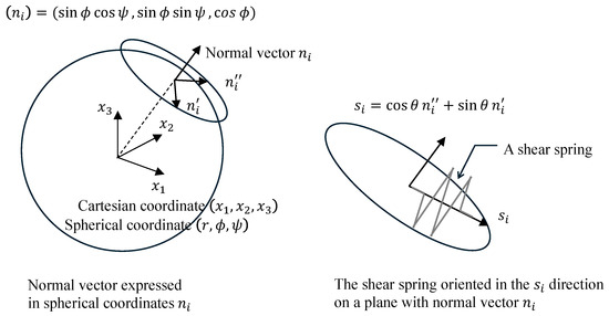
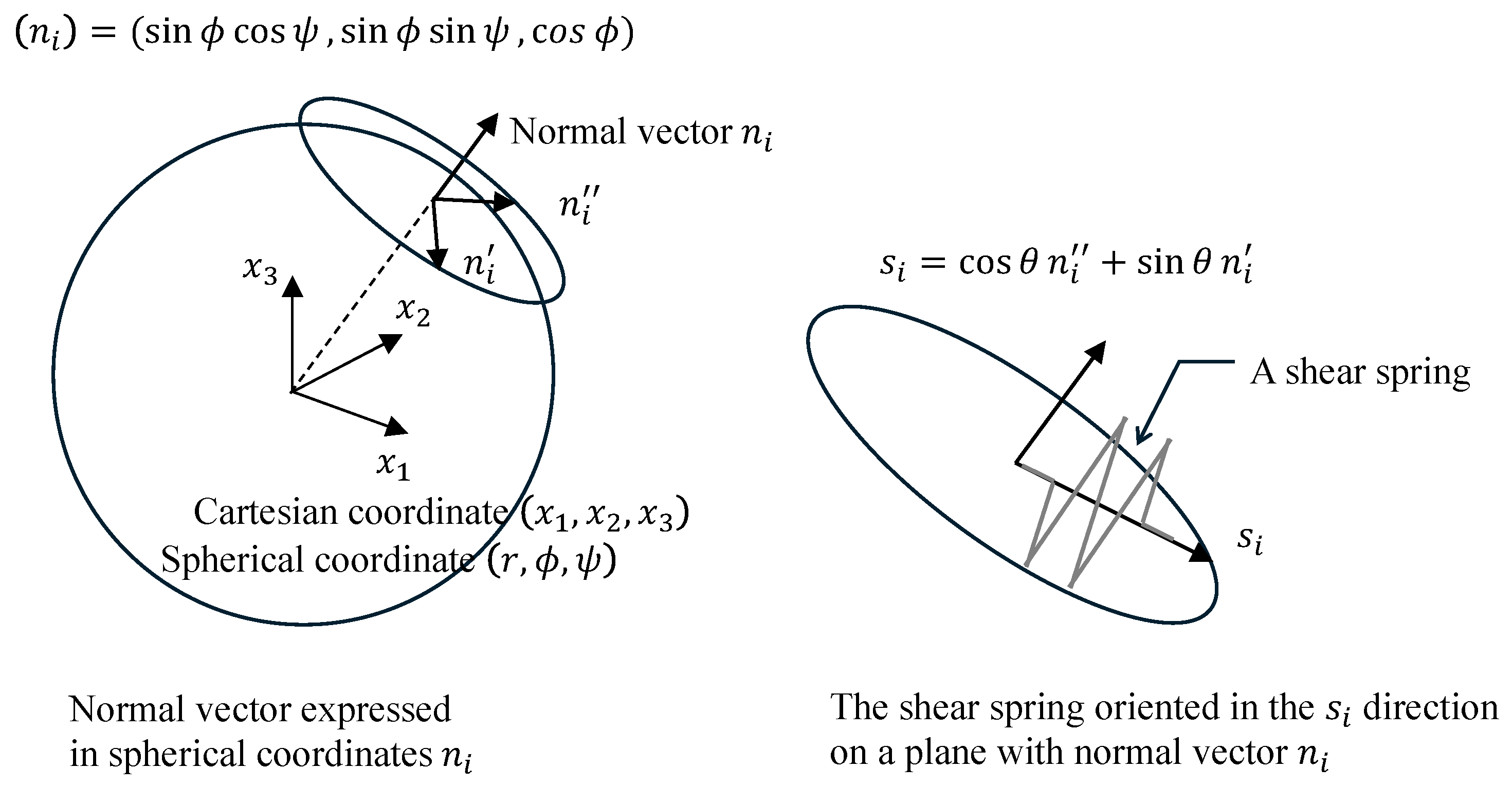
As shown in Figure 1, a cartesian coordinate system is introduced, and a plane with a normal direction given by the unit vector is considered, together with a shear spring lying on this plane. The unit vector representing the axial direction of the shear spring is denoted by . By introducing spherical coordinates , the normal vector is expressed as . A unit vector lying on the plane with normal is defined as , and another unit vector is defined as the cross product of and . The in-plane unit vector is then expressed as . Accordingly, the normal vector is represented by two variables and , while the in-plane vector is represented by a single variable .
Figure 1.
One-dimensional shear spring; Cartesian and spherical coordinate systems employed are presented.
Strain and stress tensors are denoted by and , respectively. On a plane with normal , a nonlinear spring parallel to has shear strain and stress of and . Their increments, denoted by and , satisfy the following relation:
Here, denotes the shear stiffness, which is a nonlinear function of . Note that and are expressed in terms of and , the stain and stress increment, as and . In the conventional formulation of the multiple shear mechanism model, the elasto-plasticity tensor that links to as is computed as follows:
where stands for the triple integral,
Note that the reduced model [14] is a formulation in which the one-dimensional shear spring defined by is used only once. This formulation is expressed as a double integral over and .
The reformulation of the multiple shear mechanism model starts from defining an error function of the stress increment for a given strain increment . The error of the − relationship in Equation (1) is given as . Thus, we define error function as the triple integral of the square of this error, as
that minimizes is readily determined by solving , i.e,
where and are fourth-order tensors given as
where “sym” denotes the symmetric part with respect to the index pairs and .
in Equation (6) have the following two characteristics: (1) because the triple integral is performed over all possible directions, has no directional bias and is isotropic; (2) consists only of deviatoric components derived from . Accordingly, in Equation (6) is given as
where denotes the Kronecker delta and . Note that a 4th-order tensor in the parenthesis is an isotropic tensor mapping to any 2nd-order tensor to its deviatoric tensor (that has zero volumetric part).
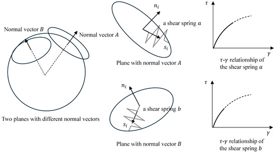
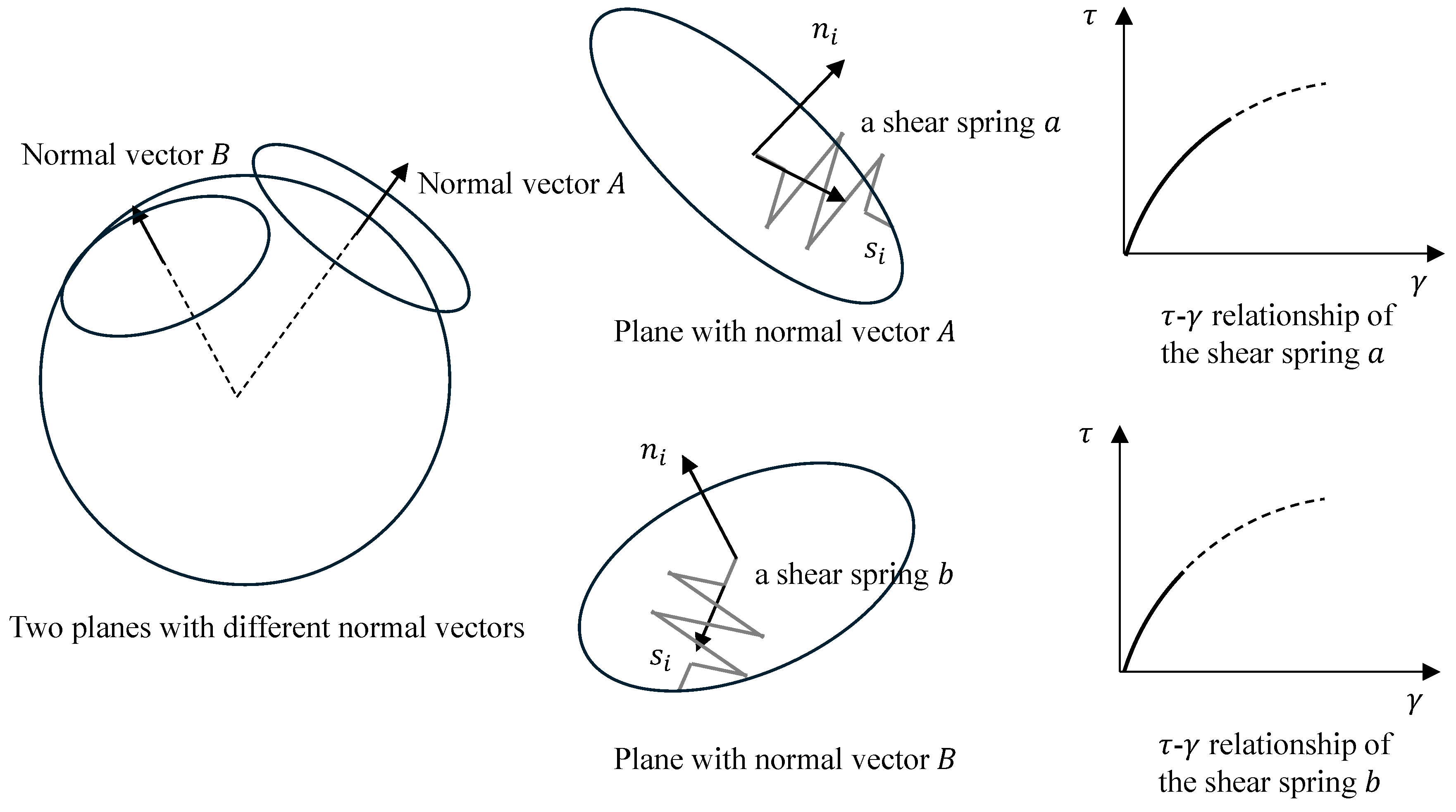
Because is a nonlinear function of , the value of differs among shear springs as shown in Figure 2. We take advantage of Taylor series expansion of at, say, . That is,
where , and . Substituting Equation (8) into Equation (6), we rewrite as
Figure 2.
Schematic illustration of the - relationships used in the multiple shear mechanism model; while the relationships is the same, the location of changes depending on the spring.
The first term on the right-hand side of Equation (9) is identical to in Equation (6). The sixth-order tensor included in the second term, , also consists of only deviatoric components derived from . Therefore, it can be evaluated analytically using isotropic tensors.
Since and are determined by Equations (7) and (9), respectively, we can compute the following elasto-plastic tensor that gives :
As shown in Equation (9), the triple integral is applied to the spring direction expressed in terms of and , unlike Equation (2) in which the product of the spring direction and of Equation (8) is triply integrated. This implies that the integrals can be evaluated analytically, in contrast to Equation (2) and to the reduced model.
Equation (10) is based on the assumption that all the springs are in loading state or unloading state. When springs in loading state and unloading state are mixed, we must separate springs since the stiffness is different. To explicitly distinguish between the loading and unloading states, the shear stiffness in Equation (1) is redefined as
where and denote the shear stiffness in the loading and unloading states, respectively. Denoting by an the domain of springs in the loading and unloading, respectively, we decompose the triple integral of Equation (3) as
For a given plane of the normal vector, we can determine the range of the spring direction on the plane for the spring in the loading and unloading states. Thus, we can compute as
where is the range of the springs in the loading and unloading states.
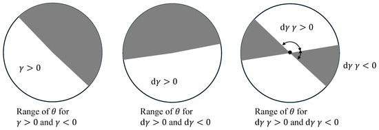
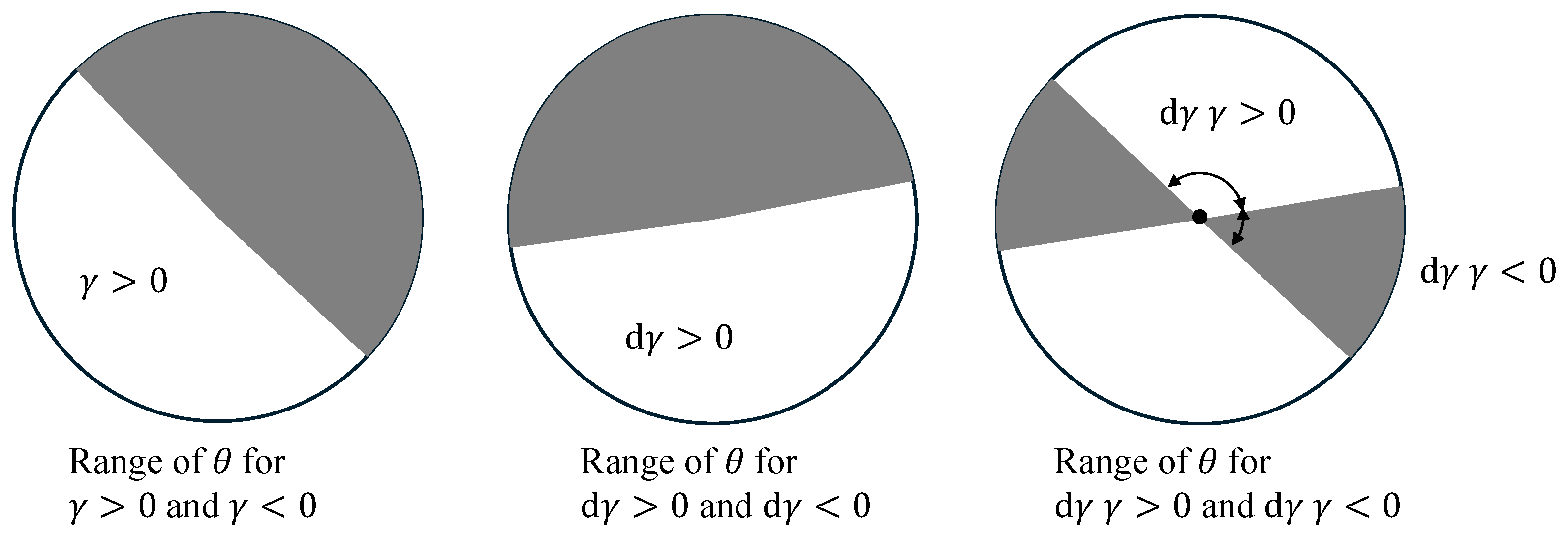
Figure 3 illustrates the classification of loading and unloading states using the range of . In the left panel, the range of is divided into and based on the sign of the shear strain computed from . In the middle panel, the range of is divided into and based on the sign of the shear strain increment computed from . In the right panel, the regions of and are superimposed, yielding the ranges of for which and . The stiffness is integrated over the range of where , whereas is integrated over the range of where . The value of at or vanishes is computed as
is thus determined by using and of Equation (14), for given and . We define and as
and obtain for the case where springs in loading and unloading coexist as
Figure 3.
Schematic illustration of and that is determined from the sign of .
Note that and are used when a Taylor series expansion is taken at . It should be noted that if a reference shear strain is adopted as the expansion point of the Taylor series, the expressions are modified as follows.
2.2. Design of Database for Triple Integral of Spring Direction
We rewrite given by Equation (15) in the following form:
where , and are 4th-, 6th- and 8th-order tensors that are computed by using triple integral,
Recall that consists of which is determined by and through Equation (14). We can rewrite in a form similar to Equation (18); 4th-, 6th- and 8th-order tensors for are determined from and of Equation (19) since , and are analytically computed.
By definition, and are computed by using the triple integral for the spring directions. If we store these 4th- and 6th-order tensors in a certain database, we can extract suitable data depending on and and compute without carrying out the triple integral at all.
The database includes the tensors for pre-determined and , and suitable interpolation is needed for the stored data to compute the right tensors for a given and As a larger number of pre-determined and is stored in the database, the interpolation gives a more accurate evaluation of and for a given and However, it requires a larger memory space in the computer node. We must design a suitable database considering the trade-off relation between the accuracy and the memory.
To reduce the size of the database, we minimize the number of indices used in the database. It is natural to use 12 components of and as the database indices, but we can reduce the number from 12 to 5. First, is transformed into a coordinate system aligned with its principal directions. Furthermore, we use only deviatoric strain and normalize it as the maximum of the absolute value of components becomes 1; if is multiplied by a positive number, of Equation (14) does not change and so does . Thus, the index number for becomes 1. Denoting the transformed component by , we introduce a three-dimensional vector and define
adding a condition of . Next, we reduce the index number for . For the transformed tensor, we use its deviatoric part and normalize it. Thus, the index number for becomes 4. Denoting the transformed component by , we introduce a six-dimensional vector and define
adding a condition of . While they are three- and six-dimensional vectors, we can assign 1 index and 4 indices to and , respectively. The range of and is and ; we presume and the second largest value of lies between 0.5 and 1. We equally divide the range of and by , and choose sets of and for which and are computed. A five-dimensional integer vector, denoted by , is determined for each set; its component ranges from 1 to .
We also reduce the number of components of and considering its symmetry. This reduction is important for memory storage, since the total number of these tensors’ component is . As for , we correspond 6 independent combinations for of to an index , so that corresponds to a six-dimensional 2nd-order tensor . Due to , satisfies and its 21 components need to be stored. Similarly, and correspond to six-dimensional 3rd- and 4th-order tensors, and , respectively. Their 56 and 126 components need to be stored due to their symmetry such as and . The sum of the stored components for , and is .
We consider the interpolation scheme for and using data extracted from the database. First, we need to extract data from the database. For given strain and strain increment, and , we compute and using Equations (19) and (20), respectively. For and , we can determine a five-dimensional real number, denoted by vector using the division of their range, and identify sets of five-dimensional integer vectors , so that is located within a five-dimensional domain determined by the sets of . For each , we extract the components of , and from the database.
A linear interpolation scheme is the simplest. The components of and for given and are computed as a linear combination of sets of the components of , and . The weight of the linear combination for each set is the product of or where denotes the discretization interval of the real-valued vectors, which is determined from the ranges of and and the number of divisions . For instance, the linear interpretation of is schematically expressed as
where and are the data and weight associated with ; or corresponds to or , respectively. If sets of the components of , and are extracted for , quadratic interpretation scheme is applicable. The weight of the linear combination needs slightly complicated computation, but and are computed more accurately.
3. Results and Discussion
3.1. Verification of Reformulated Multiple Shear Mechanism Model
In the previous study [15], we have verified the elastoplasticity tensor derived from the reformulation of the multiple shear mechanism model. A more sophisticated expression is given in this study. Therefore, we first verify the reformulated multiple shear mechanism model that uses 4th, 6th and 8th-order tensors, and , which are computed for the spring directions.
The original multiple shear mechanism model was used as a reference; the effective stress analysis program FLIP ROSE 3D was employed. A dynamic analysis of a single element was first conducted using the original model. The input ground motion was extracted from the east–west component recorded at Kurikoma, Kurihara City, Miyagi Prefecture, the 2008 Iwate–Miyagi Nairiku Earthquake; the observed strong motion data was provided by the Japan Meteorological Agency [16]. The material parameters of the multiple shear mechanism model are listed in Table 1. The material properties were determined assuming sandy soil, following the method proposed by Morita et al. [17]. The reformulated model computed a stress tensor time series for an input strain tensor time series which was calculated by the original model, and the stress tensor time series was compared with that of the original model.
Table 1.
Parameters of the multiple shear mechanism model.
In the reformulated model, the Taylor series expansion in is taken to second order and Equation (17) is thus adopted. The expansion point is chosen as the maximum shear strain among all shear springs at the previous time step. Accordingly, both and are updated at every time step.
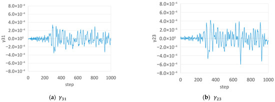
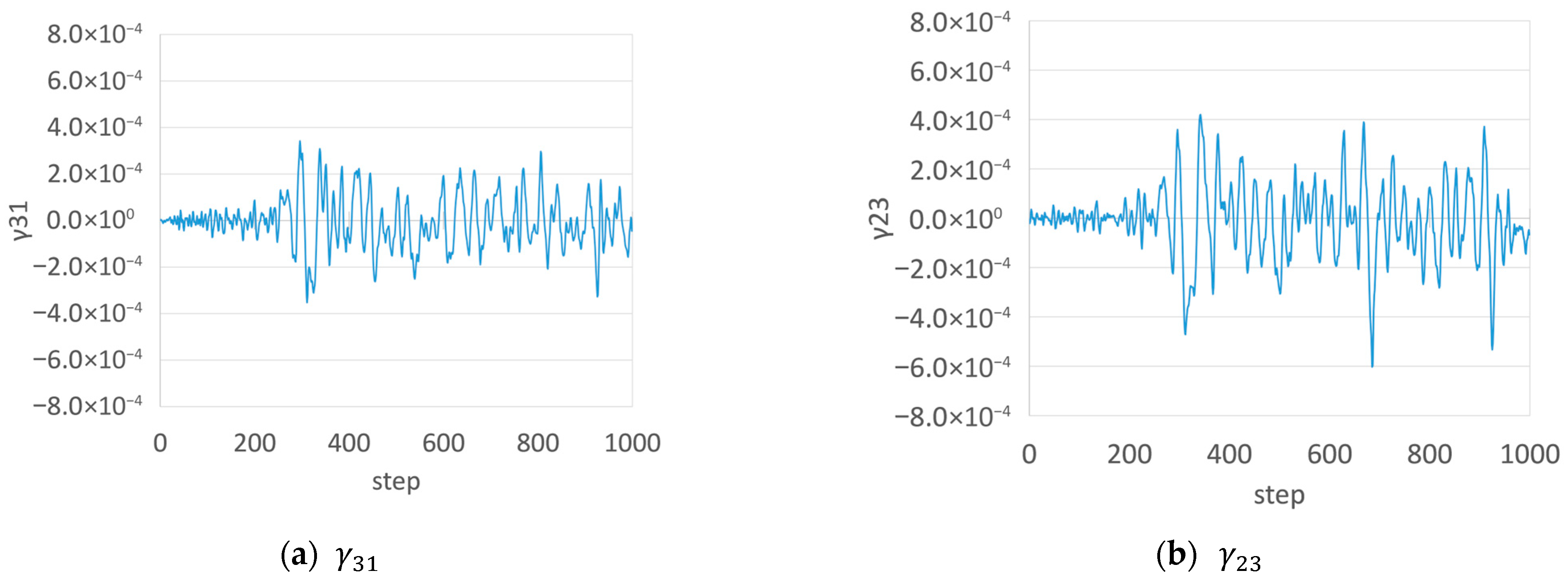
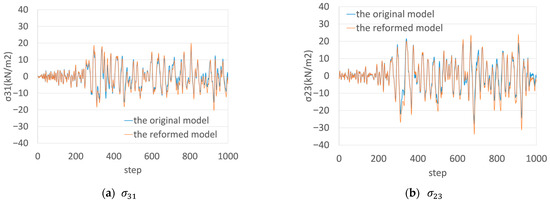
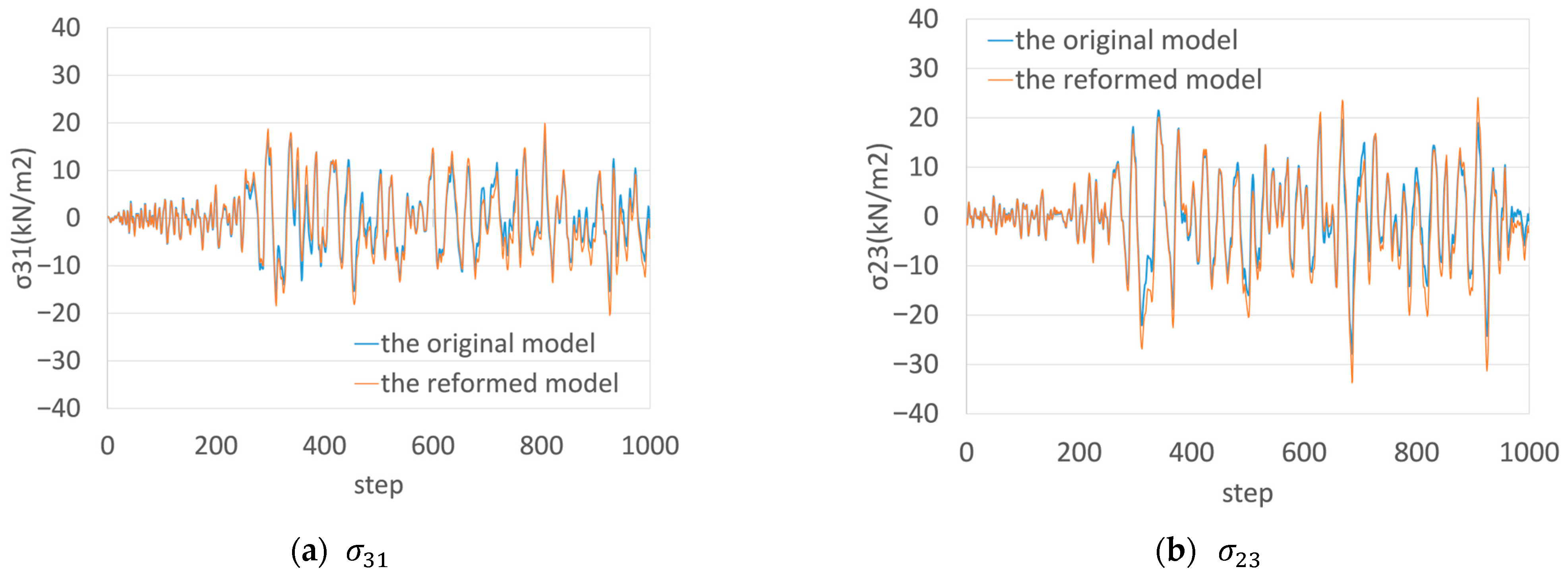
Figure 4 shows the input strain tensor time histories; two horizontal shear components are used. Figure 5 presents the stress tensor time histories for the original and reformlated models. The agreement is satisfactory.
Figure 4.
Time histories of the strain tensor input to the constitutive module.
Figure 5.
Time histories of the stress components.
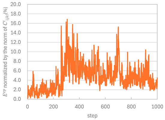
We evaluate the accuracy of the reformulated model using the norm of the difference between the elastoplasticity tensor, which is defined as
where and are the elastoplasticity tensor of the reformed and original model, respectively, and the norm is computed as . Figure 6 shows the time history of , which is normalized by the norm of .
Figure 6.
Time histories of normalized by the norm of , the error of the reformlated model’s elastoplasticity tensor.
3.2. Database Construction
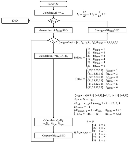
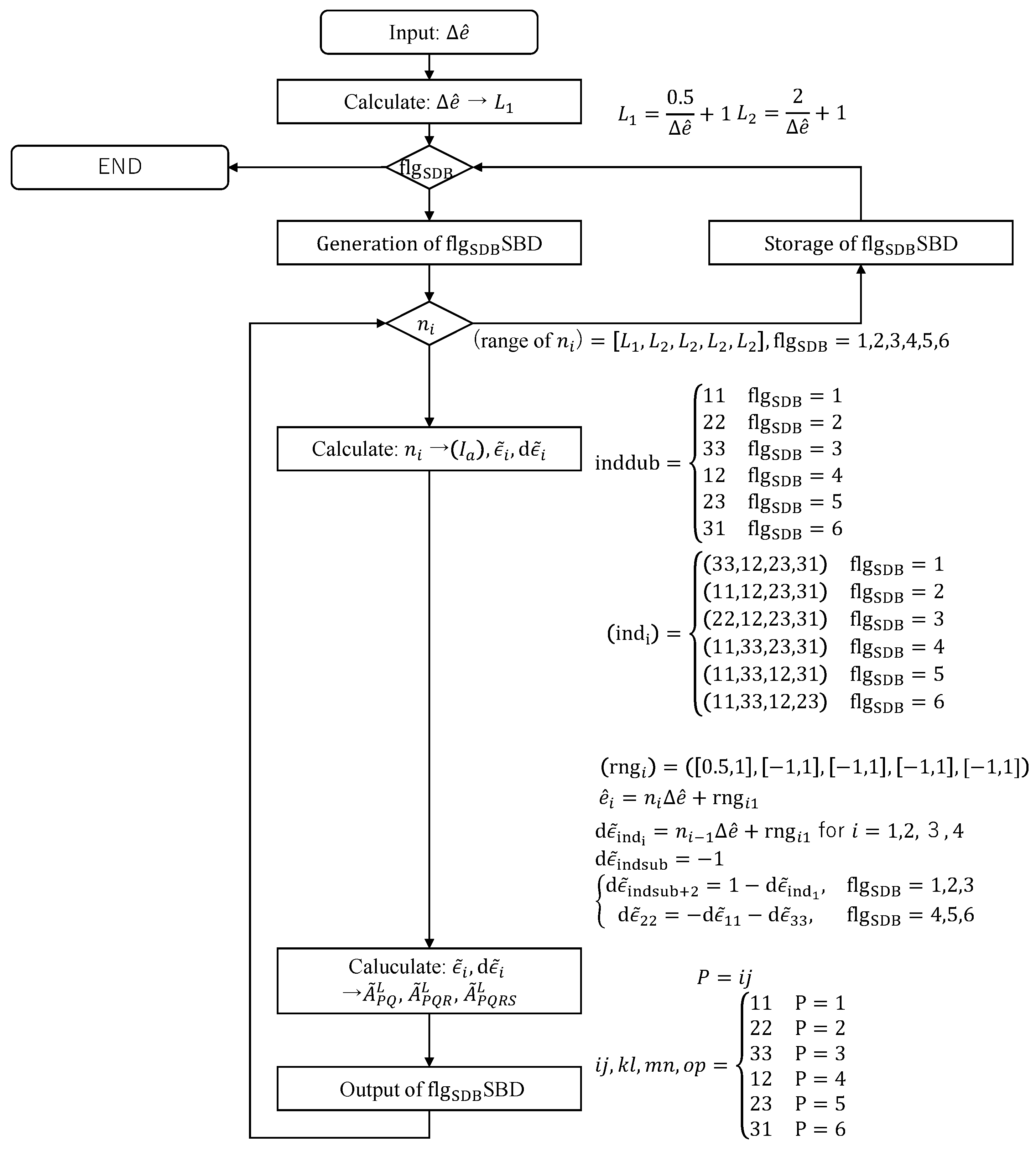
The database designed in Section 2.2 is constructed in this study. Figure 7 shows the flow of constructing database of , and . First, the number of domain division, , is transformed to the increment of and , denoted by . Corresponding to a five-dimensional integer vector, , we make five loops of generating components of and . When and are determined, we compute , and for them and store their independent components.
Figure 7.
Flow of database construction.
For more transparency, we introduce two flags, namely for a key component of and for the sign of the key component. The key component of is the component that takes on the value of or , and is the number of the key component. A sub-database is constructed for each key component. is either or , depending on the value of the key element. The sub-database is computed for the case when the key component is . Thus, for , the loading and unloading domain are whipped.
Table 2 lists the size of the database for three values of the number of domain division, or the increment of and , . The size of Database No. 1 is approximately 400 MB, which is acceptable for computer nodes with 100 ~ 200 GB memory. Note that if the twelve components of and d were used as database indices, the total number of stored tensor combinations would grow as . For (the same resolution as Database No. 1), this corresponds to tensor combinations. By reducing the number of indices, we were able to construct a database that is feasible to implement within the assumed computing environment. Due to the design studied in Section 2.2, we can locate a database for each computer node when a parallel FEM program is used in a parallel computer consisting of non-memory shared computer nodes.
Table 2.
Specifications of the database.
3.3. Database Searching and Referencing
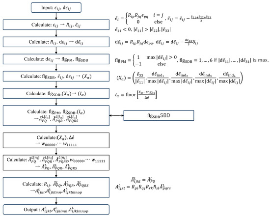
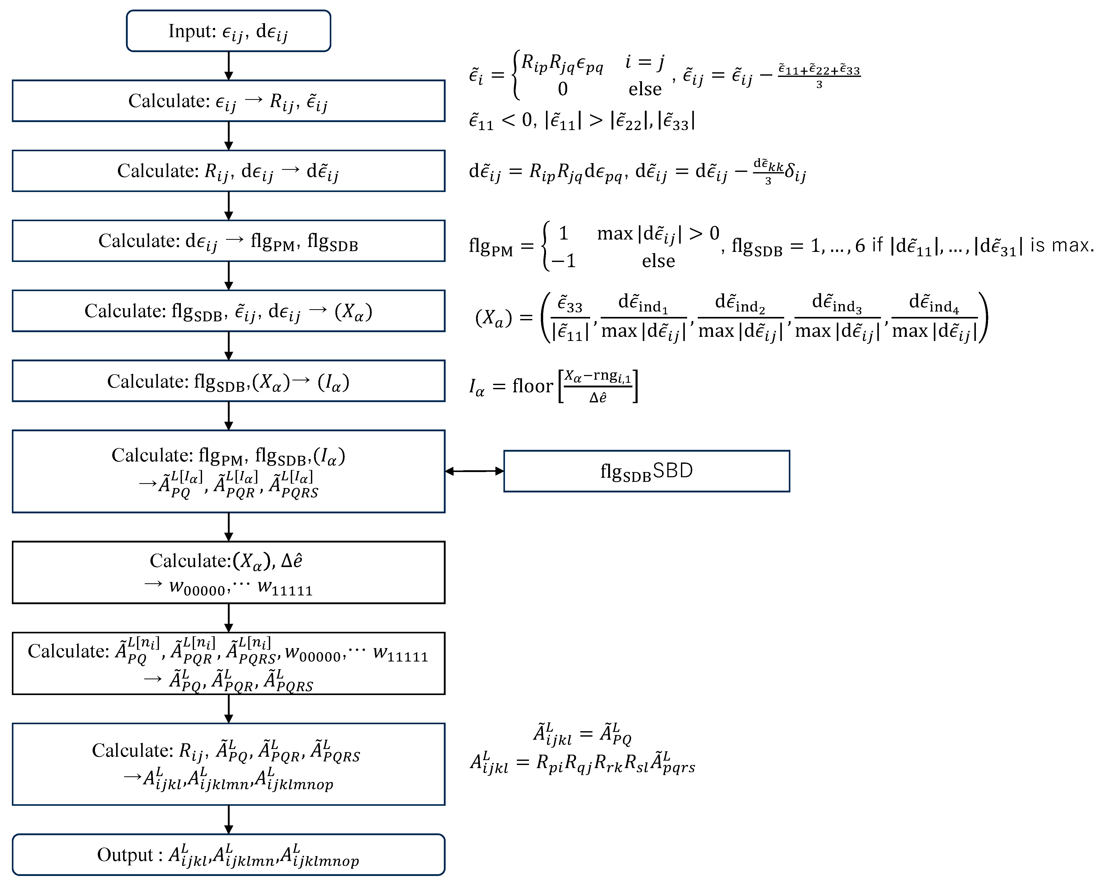
Figure 8 shows the flow of database searching and referencing. For given and , the flow shows a sequence of arriving at a five-dimensional real number vector , from which a set of five-dimensional integer vectors are obtained by applying floor or ceiling functions to . Each is used as a search parameter of the database. As described previously, the database is implemented as sub-databases. Note that the sub-database is first selected by determining , a flag for the key component of , together with , a flag for the sign of the key component.
Figure 8.
Flow of database searching and referencing.
Because a five-dimensional integer vector is used as a search parameter for the database, the location of data can be hashed, and a hash table is adopted as the data structure of the database [18]. The computational complexity required for searching a hash table is , which significantly reduces the computational cost of database searches.
3.4. Examination of Computational Performance Increase Using Database
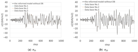
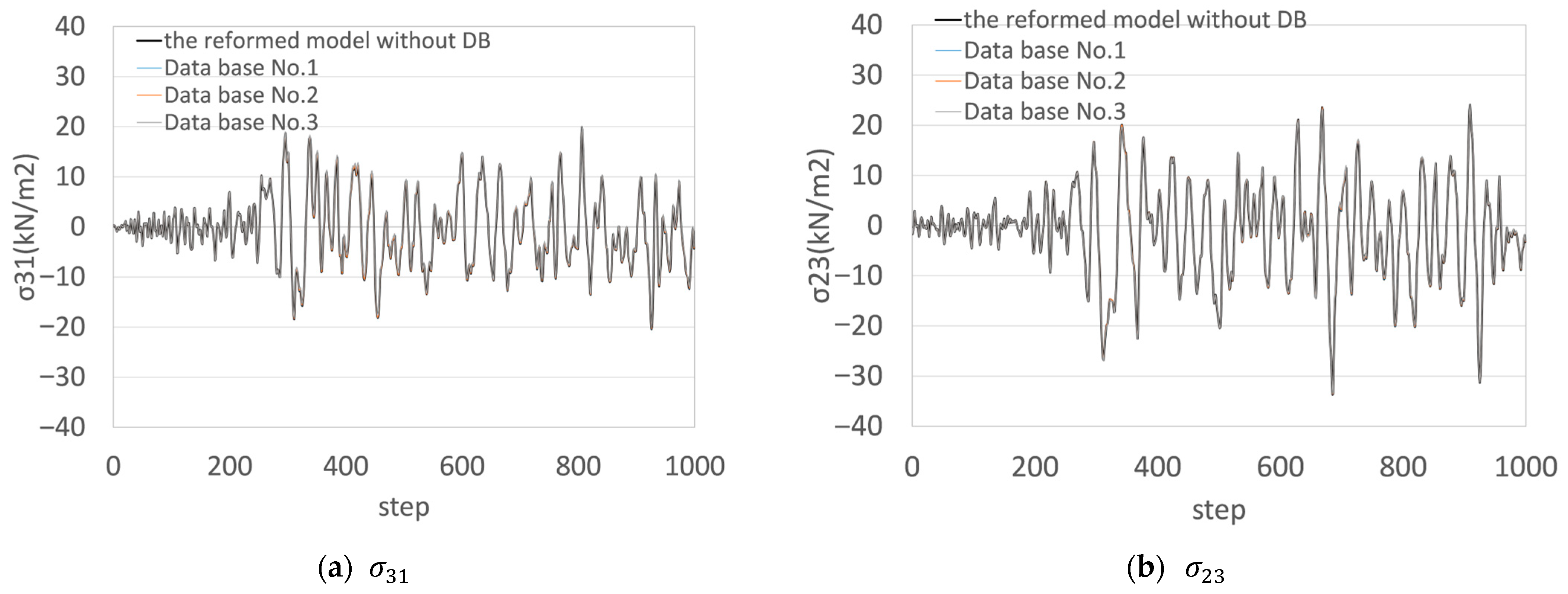
Figure 9 shows the time histories of the stress components. The numerical experiments were conducted on a workstation equipped with an Intel Xeon Gold 6246 CPU (Santa Clara, CA, USA). The system memory consisted of DDR4-2933 RAM. Data storage was provided by SATA-connected solid-state drives with a nominal read speed of 540 MB/s, configured in a RAID 5 array.
Figure 9.
Time histories of the stress components.
The results obtained using the reformulated model with the database are in good agreement with those of the reformulated model without DB. No significant differences in the results were observed among the databases with different resolutions.
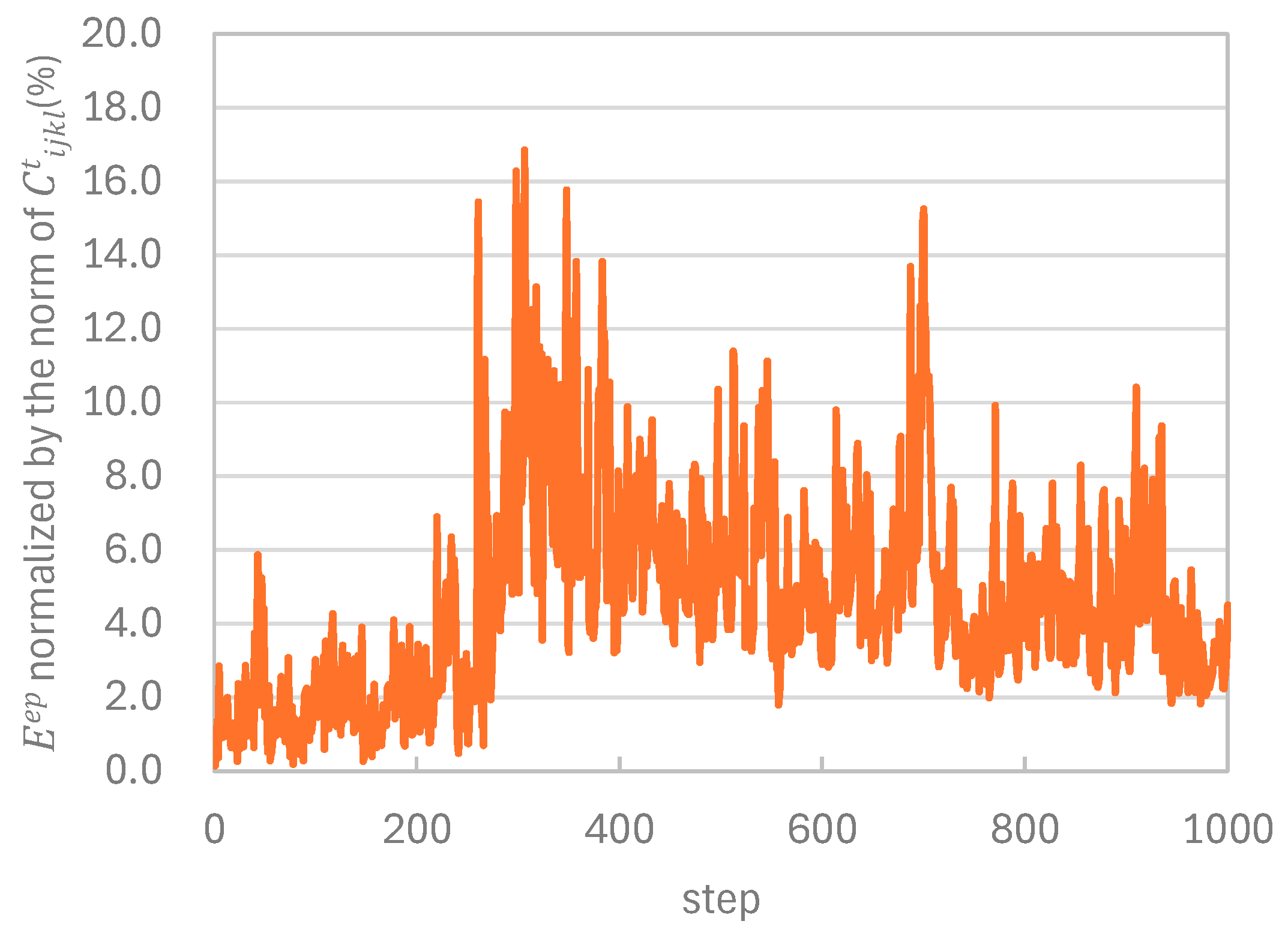
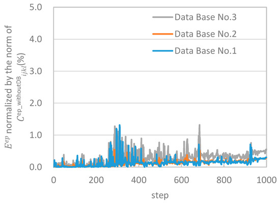
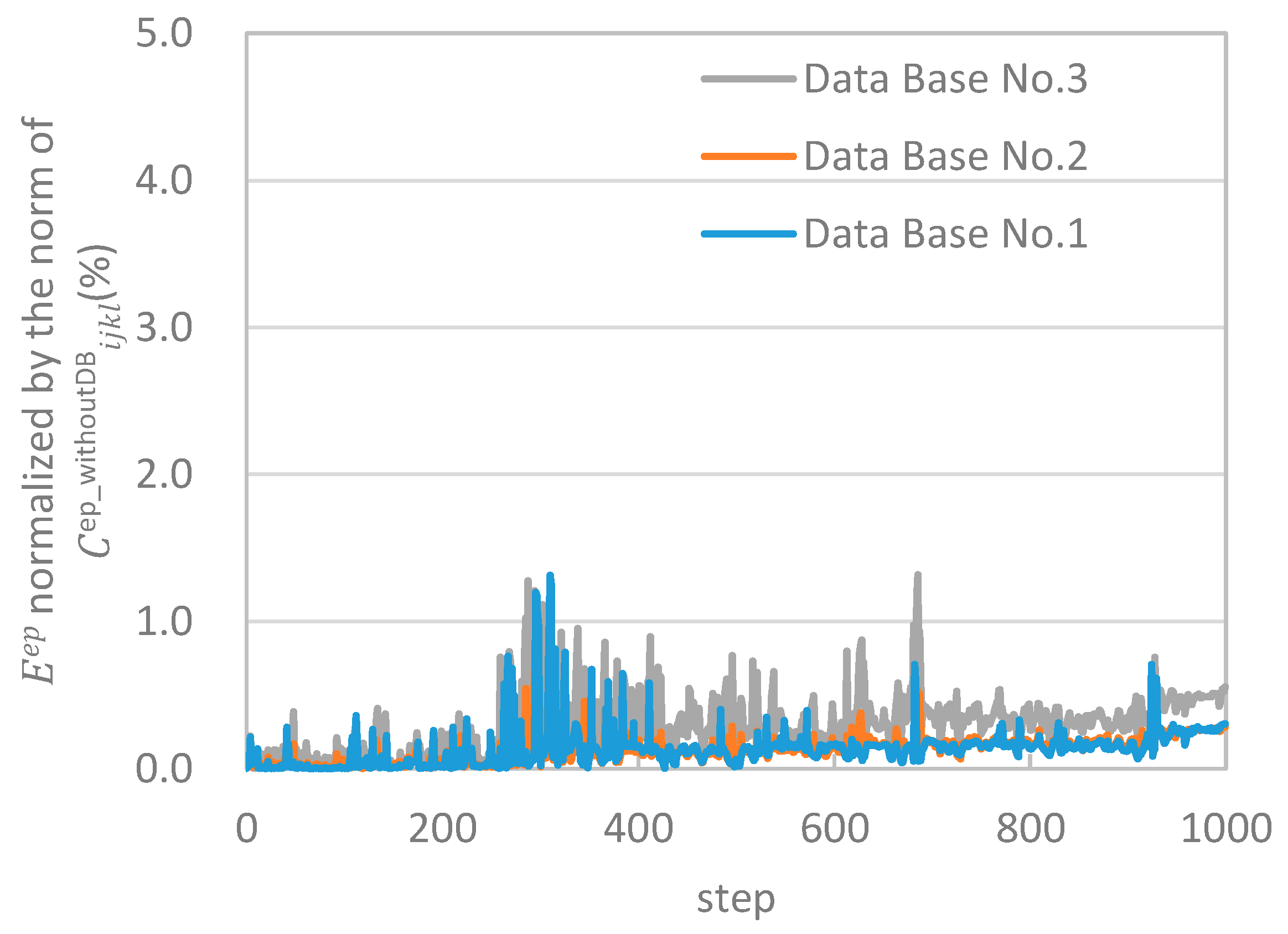
Figure 10 shows the time histories of the relative error computed from the norm of the difference between the elastoplasticity tensors. The approximation accuracy of the database-based computation was evaluated in terms of the relative error with respect to the reformulated model without the database. The relative error reached a maximum of approximately +1%. On the other hand, for Database No. 3, which has the lowest resolution, the relative error with respect to the reference solution tended to exhibit stronger discontinuities. The observed discontinuities in the relative error coincide with times at which the magnitude of the response change increases sharply. When the change in response is large, the integration range for the springs changes abruptly, causing the tensor components based on triple integrals of to vary suddenly as well. Database No. 3, which has relatively low resolution, could not smoothly track these rapid changes in the tensor components; this inability is therefore considered to be the cause of the pronounced discontinuities in the error.
Figure 10.
Time histories of normalized by the norm of .
In all cases, the error showed a tendency to accumulate in the latter part of the loading process. However, the magnitude of the relative error was sufficiently small that it did not explicitly appear in the time histories of the stress components. Its practical influence is therefore considered negligible. In particular, the relative error for Database No. 1 remained approximately constant. This indicates that the accumulation of error was relatively suppressed. The final error was also less than 0.5%.
Table 3 compares the computational times of the reformulated model without the database and the reformulated model with the database.
Table 3.
Comparison of computational time.
The computational time of the reformulated model with the database was reduced to approximately 2% of that of the reformulated model without the database. The difference between the two models lies in the treatment of the higher-order tensors required for the Taylor expansion. In one case, these tensors are computed sequentially by the CPU, whereas in the other case they are retrieved from the database stored in memory. By eliminating the computation of triple integrals, the CPU computational load is reduced, resulting in a significant reduction in computational time.
On the other hand, a comparison among the reformulated models using different database resolutions was conducted. The computational time tended to increase as the database resolution increased. This difference is attributed to the time required to load the database from storage into memory at the beginning of the computation. When the database loading time is excluded, the computational time is almost the same regardless of the database size.
Based on the above results, the database reformed in this study has the following characteristics.
First, as the database resolution increases, the database loading time increases. However, the loading process is performed only once, and the required time is on the order of a few seconds. This time is negligibly small compared with the computational time required for three-dimensional analyses.
Second, because a hash table is adopted for the database search algorithm, the computational complexity of searching is always . The computational cost of database searching does not depend on the database resolution. Therefore, the computational time required to evaluate the elastoplasticity tensor is independent of the database resolution.
3.5. Applicability and Future Work
In this study, the verification was conducted using a database in which interpolation was performed by linear interpolation. Among the databases examined, Database No. 1 (with an increment of 0.25) exhibited the smallest interpolation error. At the same time, a sufficient reduction in computational time was achieved. Under these conditions, the influence of the database size on the computational time is considered to be small.
In future work, the reformulated model will be implemented in a parallel finite element method for further verification. We will initially implement the model using MPI-based distributed-memory parallelization. In this implementation, the database will be stored in a simple replicated fashion, with each MPI process maintaining its own copy. This straightforward replication strategy simplifies data access during tensor retrieval and avoids inter-process communication [19]. Under the assumed computing environment, Database No. 1 (≈400 MB) can be operated without difficulty.
If the resolution of Database No. 1 is doubled (i.e., the number of discretization points is doubled), the database size increases to approximately 5 GB. At a resolution of 2.5 times ( = 0.1), the database size increases to approximately 20 GB. When implemented with MPI-based distributed-memory parallelization, the database is replicated according to the number of parallel processes. As a result, even with a moderate degree of parallelism, the replicated databases may occupy a substantial portion of the available memory on a computing node. Considering the additional memory required for storing stiffness matrices and other data structures in large-scale finite element analyses, databases on the order of GB become difficult to implement in practice. From a practical viewpoint, Database No. 1 is therefore considered to provide the best balance between approximation accuracy and memory efficiency within the range of available computing environments. In higher-performance computing environments, this limitation may be alleviated. Moreover, when implemented using OpenMP with shared memory, a larger database can be used because replication across processes is not required [20].
The objective of this study is to verify the effectiveness of the database in reducing the computational time. A comparison with the conventional formulation of the multiple shear mechanism model is left for future work. Such a comparison can be conducted by implementing the constitutive module used in this study into a finite element method framework. In Appendix A, we present a comparative verification between the original model and the reformulated model under the limited condition of a single parallel process and a single finite element. Under this constrained configuration, the reformulation reduces computational time compared with the original formulation.
4. Conclusions
The conclusions of this study are summarized as follows:
- In a previous study, a reformulation of the multiple shear mechanism model was proposed. In this reformulation, the triple integrals are expressed using integrals of . In the present study, a database-based method was proposed, in which the strain tensor and the strain increment tensor were used as search parameters. In the database, tensors obtained from the integrals of under various conditions are stored;
- To minimize the database size, methods for reducing the number of search parameters and the number of stored tensor components were proposed. In addition, interpolation was applied to the tensor computation to maintain sufficient accuracy. The procedures for database construction and database searching were also organized;
- The size of the designed database was approximately 400 MB. This database size satisfies the performance requirements of the target computing environment. The applicability of the reformed methods for reducing the number of search parameters and stored tensor components was demonstrated;
- The reformulated model successfully reproduced the time histories of stress obtained by the reformulated model without the database. The relative error of the norm of the difference between the elastoplasticity tensors was approximately 1%. These results demonstrate that the proposed method has sufficient approximation accuracy;
- The reformulated model reduced the computational time to approximately 2% of that required by the reformulated model without the database. In this case, the influence of the database size on the total computational time was shown to be small. The results demonstrate that computational acceleration was achieved by using a database in which tensors obtained from the integrals of under various conditions are stored;
- This study focuses on verification at the level of the constitutive module. Implementation into a finite element method framework and comparison with the conventional formulation of the multiple shear mechanism model are left for future work. The reformulated model, constructed as a constitutive module, can be readily implemented into finite element analyses. It should be noted that, as demonstrated in Appendix A, the reformulated model produced results indicating that it can reduce computational time relative to the conventional formulation.
- It should be noted that this investigation was carried out under the limited condition of a single parallel process and a single finite element. The assembly of the stiffness matrix and the processing of boundary conditions are expected to account for a large proportion of the computation time. Comparative verification at model scales representative of practical engineering applications remains a subject for future work.
Author Contributions
Conceptualization: M.H.; methodology, M.H.; software, Y.S.; validation, Y.S.; formal analysis, Y.S.; writing—original draft preparation, Y.S. and W.H.; project administration, M.H. and W.H. All authors have read and agreed to the published version of the manuscript.
Funding
This research received no external funding.
Data Availability Statement
Data are contained within the article.
Conflicts of Interest
Authors Yoshihiro Shishikura and Wataru Hotta were employed by the company TAISEI CORPORATION. The remaining authors declare that the research was conducted in the absence of any commercial or financial relationships that could be construed as a potential conflict of interest.
Appendix A
The reformulated model was implemented into a finite element method and verified against the original model. The verification focuses on a comparison of computational time and response results. Both models were implemented using the E-FrontISTR finite element method. Note that the tests were executed using a single parallel process (i.e., no parallel computation was performed). The numerical experiments were conducted on a computing system (compute nodes equipped with Intel Xeon Gold 6246 CPUs and DDR4-2933 system memory).
The dynamic analysis target was a single finite element representing a 1 m cubic specimen. Material properties are the same as those used in Section 3.1. The analysis procedure consisted of an initial stress analysis to introduce a mean effective stress of , followed by a dynamic analysis.
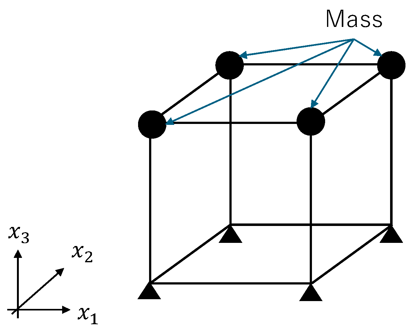
Boundary conditions for the dynamic analysis are shown in Figure A1. The bottom face of the element was fully fixed. The four nodes on the top face were constrained in the vertical direction, while horizontal displacements in the two lateral directions were constrained to be identical. To simulate seismic response under full-stress conditions, lumped masses were attached to the four top nodes so that the maximum shear strain arising in the element is approximately . The total mass of the lumped particles was 3 t.
Figure A1.
Schematic of the 1 m cubic single-element test model and boundary conditions.
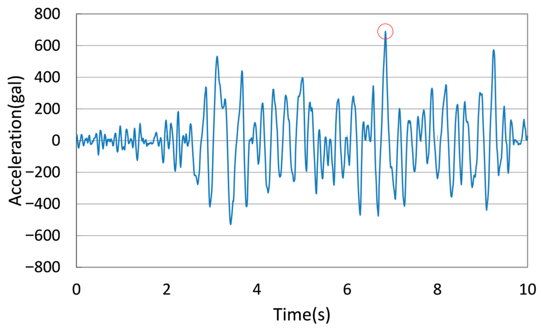
The input seismic motion is a 10 s segment extracted from the strong-motion record at Kurikoma, Kurihara City, Miyagi Prefecture, during the 2008 Iwate–Miyagi Nairiku Earthquake (strong-motion data provided by the Japan Meteorological Agency). The seismic motion was applied in a single horizontal direction. The time step was 0.01 sec/sec, and the total number of steps was 1000 (Figure A2).
Figure A2.
Input seismic motion (horizontal). The red circle indicates the time at which the peak acceleration occurs.
Settings for the reformulated model are as follows. Database No. 1 was used and interpolation was linear. The Taylor series expansion in was taken to zeroth order (constant term only), and the expansion point was chosen as the maximum shear strain among all springs at the previous time step. Accordingly, both and were updated at every time step.
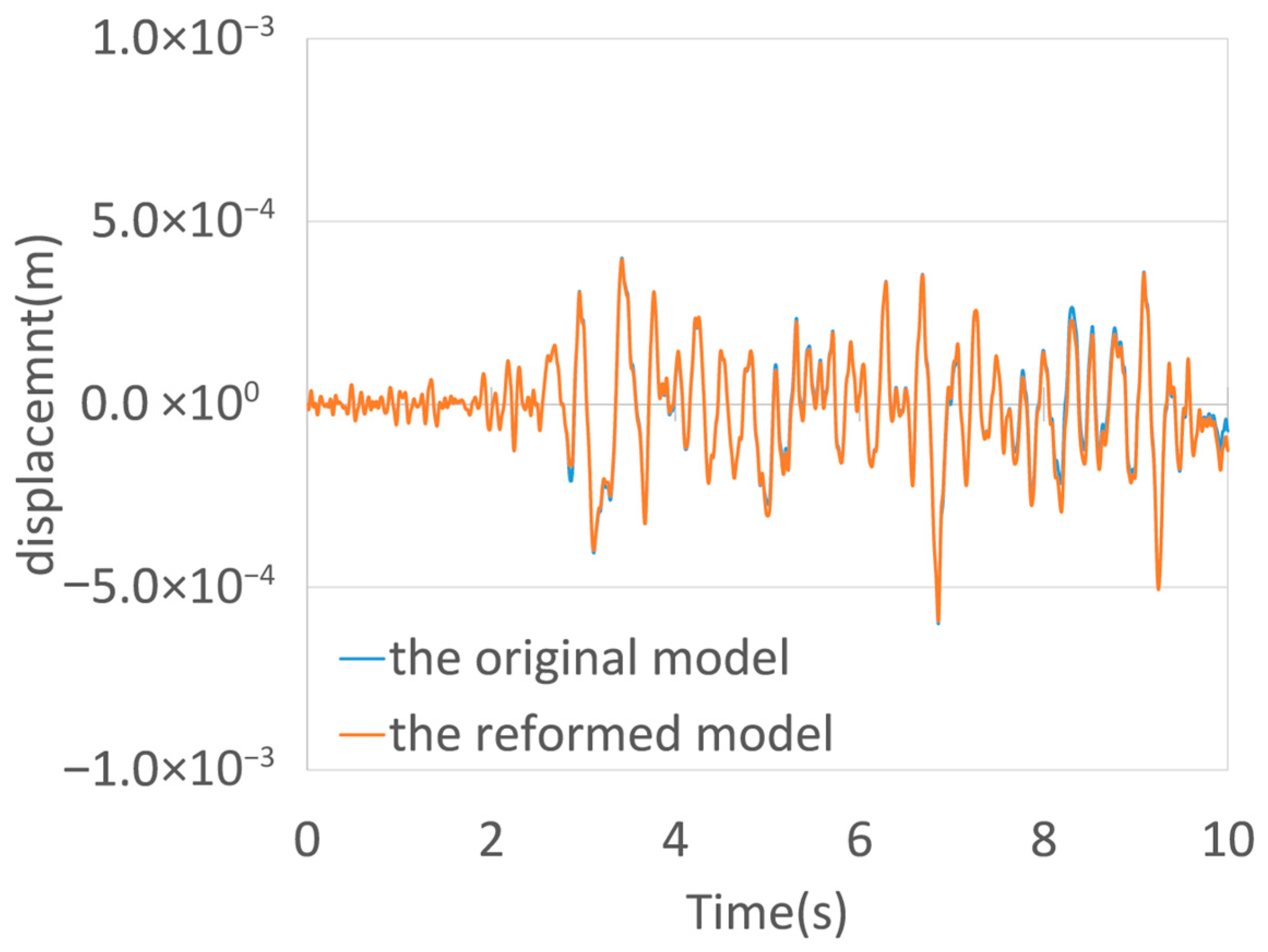
Figure A3 shows the time histories of the horizontal displacement components at the top of the model. The reformulated model is in good agreement with the original model. Moreover, the computational time was 18.34 s for the original model and 12.47 s for the reformulated model. Thus, the computational time was reduced to approximately 70% of the original.
Figure A3.
Time histories of the horizontal displacement components at the top of the model.
References
- Towhata, I.; Ishihara, K. Modelling soil behavior under principal stress axes rotation. In Proceedings of the 5th International Conference on Numerical Methods in Geomechanics, Nagoya, Japan, 1–5 April 1985; Volume 1, pp. 523–530. [Google Scholar]
- Iai, S. Micromechanical background to a strain space multiple mechanism model for sand. Soils Found. 1993, 33, 102–117. [Google Scholar] [CrossRef] [Scilit]
- Hardin, B.O.; Drnevich, V.P. Shear modulus and damping in soils: Design equations and curves. Proc. Am. Soc. Civ. Eng. 1972, 98, 667–692. [Google Scholar] [CrossRef] [Scilit]
- Datta, T.K. Seismic Analysis of Structures; Wiley: Hoboken, NJ, USA, 2010; ISBN 9780470824610. [Google Scholar]
- Hashash, Y.M.A.; Hook, J.J.; Schmidt, B.; Yao, J.-I.-C. Seismic design and analysis of underground structures. Tunn. Undergr. Space Technol. 2001, 16, 247–293. [Google Scholar] [CrossRef] [Scilit]
- de Borbón, F.; Domizio, M.; Ambrosini, D.; Curadelli, O. Influence of various parameters in the seismic soil–structure interaction response of a nuclear power plant. Eng. Struct. 2020, 217, 110820. [Google Scholar] [CrossRef] [Scilit]
- Zucca, M.; Valente, M. On the limitations of decoupled approach for the seismic behaviour evaluation of shallow multi-propped underground structures embedded in granular soils. Eng. Struct. 2020, 211, 110497. [Google Scholar] [CrossRef] [Scilit]
- JSCE Committee. Seismic Performance Verification Guidelines for Critical Underground Reinforced Concrete Structures in Nuclear Plants—2021—(English Draft); Japan Society of Civil Engineers: Tokyo, Japan, 2023; Available online: https://committees.jsce.or.jp/ceofnp/system/files/Guidelines2021DRAFT20230804.pdf (accessed on 29 January 2026).
- Shimabata, T.; Matsuo, T.; Morozumi, H.; Shimamura, S. Evaluation on seismic response behavior for RC underground structure using 3D material nonlinear analysis. J. Struct. Eng. A 2020, 66A, 231–241. [Google Scholar]
- Guan, J.; Gao, Z.; Zhao, M.; Du, X. Seismic Response Analysis of Buried Nuclear Power Plant Structures in Non-Bedrock Sites. Appl. Sci. 2025, 15, 4378. [Google Scholar] [CrossRef] [Scilit]
- Motoyama, H.; Sawada, M.; Hotta, W.; Haba, K.; Otsuka, Y.; Akiba, H.; Hori, M. Development of a general-purpose parallel finite element method for analyzing earthquake engineering problems. Earthq. Engng. Struct. Dyn. 2021, 50, 4180–4198. [Google Scholar] [CrossRef] [Scilit]
- Otsuka, Y.; Tamari, Y.; Fujita, K.; Ichimura, T. Hazard map for liquefaction by 3D seismic response analysis using the supercomputer “Fugaku”. Jpn. J. JSCE 2024, 80, 23-13107. [Google Scholar] [CrossRef] [Scilit]
- Iai, S. Three-dimensional formulation and objectivity of a strain space multiple mechanism model for sand. Soils Found. 1993, 33, 192–199. [Google Scholar] [CrossRef] [Scilit]
- Hotta, W.; Suzuki, S.; Hori, M. On contraction of a three-dimensional multiple shear mechanism model for evaluation of large-scale liquefaction using high-performance computing. Geosciences 2019, 9, 38. [Google Scholar] [CrossRef] [Scilit]
- Shishikura, Y.; Hotta, W.; Hori, M. Reformulation of the multiple shear mechanism model for faster numerical analysis. J. JSCE Spec. Issue (Appl. Mech.) 2026, in press. [Google Scholar]
- Japan Meteorological Agency (JMA). Strong Motion Observation Data. Available online: https://www.data.jma.go.jp/eqev/data/kyoshin/jishin/ (accessed on 15 March 2024).
- Morita, T.; Iai, S.; Hwang, L.; Ichi, K.; Sato, Y. Simplified Method to Determine Parameters of FLIP; No. 869; Technical Note of the Port and Harbour Research Institute, Ministry of Transport: Yokosuka, Japan, 1997. [Google Scholar]
- Medjedovic, D.; Tahirovic, E.; Dedovic, I. Algorithms and Data Structures for Massive Datasets; Manning: Shelter Island, NY, USA, 2022. [Google Scholar]
- Alheit, B.; Peirlinck, M.; Kumar, S. COMMET: Orders-of-magnitude speed-up in finite element method via batch-vectorized neural constitutive updates. arXiv 2025, arXiv:2510.00884. [Google Scholar] [CrossRef] [Scilit]
- Dagum, L.; Menon, R. OpenMP: An industry-standard API for shared-memory programming. IEEE Comput. Sci. Eng. 1998, 5, 46–55. [Google Scholar] [CrossRef] [Scilit]

Disclaimer/Publisher’s Note: The statements, opinions and data contained in all publications are solely those of the individual author(s) and contributor(s) and not of MDPI and/or the editor(s). MDPI and/or the editor(s) disclaim responsibility for any injury to people or property resulting from any ideas, methods, instructions or products referred to in the content. |
© 2026 by the authors. Licensee MDPI, Basel, Switzerland. This article is an open access article distributed under the terms and conditions of the Creative Commons Attribution (CC BY) license.