Abstract
In earthquake engineering, acceleration has played a major role, while wave energy has rarely been considered as a demand in design. In order to understand earthquake damage mechanism in terms of energy, the demand in terms of wave energy in surface soil layers is studied here, assuming one-dimensional SH wave propagation by using a number of vertical array records during nine strong earthquakes in Japan. A clear decreasing trend of the energy demand with decreasing ground depth and decreasing surface soil stiffness has been found as well as a propensity of incident energies calculated at bedrocks being roughly compatible with empirical formulas. How the energy demand is correlated with structural damage is also discussed in simplified models to show that induced structural strain is governed by upward energy flux, degree of structural resonance, and impedance ratio between structure and ground and structural stiffness. In low-damping brittle superstructures, wave energy flux in resonance and associated predominant frequency are decisive in determining the damage, while cumulative wave energy determines the damage in high damping ductile soil and massive concrete structures. The trend of lower energy demand in softer soil sites may not be contradictory, with a widely accepted perception that softer soil sites tend to suffer heavier earthquake damage as far as geotechnical damage is concerned.
1. Introduction
Seismic design in practice is based on inertia force given by acceleration (e.g., maximum or equivalent acceleration) or seismic coefficients. The concept of seismic coefficient was probably first started by Sano in 1917 [1] and was employed in developing building codes after the 1923 Great Kanto earthquake, which killed about 140 thousand people in metropolitan Tokyo. This was followed by force-based design methodologies using peak values of accelerations or their spectral intensities, such as by Housner (1952) [2].
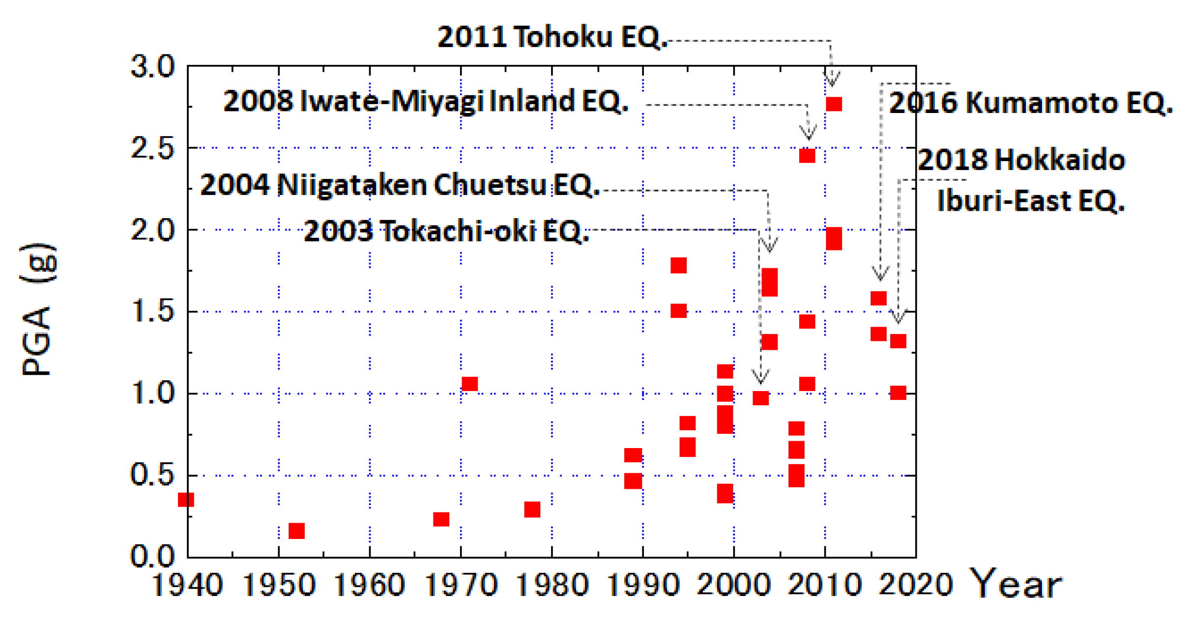
Although the force-based design method has long been used to date, it is increasingly recognized that acceleration alone may not be an appropriate parameter for seismic damage evaluation. More and more strong acceleration records with a maximum value far exceeding 1 g have been obtained in recent years. Figure 1 summarizes horizontal peak ground accelerations (PGAs) observed during recent strong earthquakes until 2021 mainly in Japan. The PGA values have increased considerably as the years go by, arriving at nearly 3 g. This is presumably because the density of earthquake observation networks (for example K-NET and KiK-net by NIED, Japan [3]) are becoming denser in their deployments to be able to pick up localized higher PGAs than before.
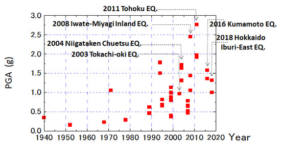
Figure 1.
PGAs observed during strong earthquakes in recent years mainly in Japan.
Conversely, cases are increasing where no significant structural damage was reported despite observed high PGAs, e.g., 1.8 g in Tarzana, California during the 1994 Northridge earthquake, United States of America; 1.7 g in Tokamachi during the 2004 Niigata-ken Chuetsu earthquake Japan; and 2.8 g in Tsukidate during the 2011 Tohoku earthquake Japan, etc. Particle velocity has been increasingly used recently in addition to the acceleration because it is believed to be closely related to induced strain and wave energy. This energy concept was employed by seismologists (Gutenberg and Richter 1942 [4], 1956 [5], Gutenberg 1956 [6]) in order to evaluate the total energy released from a seismic source based on observed earthquake records assuming spherical energy radiation for body waves. However, from the viewpoint of engineering design, in particular, only a few researchers tried to investigate earthquake motions in terms of energy. Among them, Sarma (1971) [7] calculated site specific seismic energies from velocity records and compared them with spherically radiated energy from the earthquake source. In seismically induced liquefaction evaluation, energy-based methods have been proposed, where the energy capacity for liquefaction triggering was compared with earthquake energy demand (Davis and Berrill 1982 [8]), although it is scarcely used in practice.
In most of these investigations, the energy concept is restricted in the energy capacity of soils and structures, while the energy demand in design earthquakes has scarcely been discussed. Kokusho and Motoyama (2002) [9] performed a basic study on the energy demand of seismic waves in surface layers based on one-dimensional multi-reflection theory of SH waves using vertical array records during the 1995 Kobe earthquake, which was followed by theoretical study on the same topic by Kokusho et al., (2007) [10]. Similar studies using a number of vertical array data were further carried out to understand general trends of energy demand in surface layers (Kokusho and Suzuki 2011 [11], 2012 [12]).
In the following sections, the energy demands in surface soil layers are discussed based on the calculations of wave energy flows in basic simple models and actual soil profiles of vertical array sites using the multi-reflection theory of one-dimensional SH wave propagations.
2. Energy Flow of One-Directionally Propagating SH Wave
The displacement u in SH wave propagating to the positive direction of z-axis as illustrated in Figure 2 can be expressed in the following form.
Here, t = time, z = upward coordinate, Vs = S-wave velocity, A = wave amplitude, and f (·) is an arbitrary function. Then, Equation (2) is readily obtained as a basic relationship where shear strain , and particle velocity (e.g., Kokusho 2017 [13]).
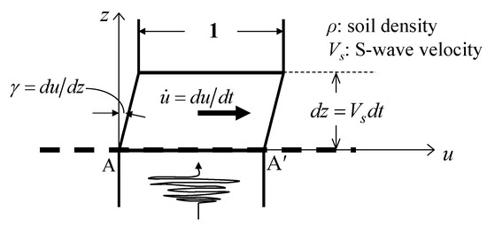
Figure 2.
Schematic illustration of wave energy in upward SH wave propagation.
As for the wave energy carried by the upward SH wave passing through a horizontal plane A-A′ of a unit area, kinetic energy can be written as Equation (3) in a soil element of a unit horizontal area times a small thickness (a travel distance in a short time increment ) having particle velocity .
Strain energy is expressed simultaneously by shear stress and shear strain γ, and using Equation (2) as:
Hence, holds in the same soil element, and the wave energy passing through the unit area in the time increment is their sum expressed as:
Cumulative energy in a time interval t = t1~t2 can be expressed as the sum of the kinetic and strain energies, Ek and Ee, of the equal amount (Timoshenko and Goodier 1951 [14], Bath 1956 [15], Sarma 1971 [7]) as:
Note that the unit of E is Energy divided by Area, and kJ/m2 will be used hereafter. Time derivative of the energy called as energy flux or energy flow rate is written as:
Thus, the seismic wave energy is dependent not only on the wave amplitude in particle velocity, but also on the S-wave impedance of the soil where the ground motion is recorded. In this context, it is meaningless from the viewpoint of energy to define design motions, acceleration or velocity, without specifying the associated impedance value . Hence, when a design motion with a given amplitude is discussed, it is essential to identify the impedance value or soil condition where the motion is defined.
2.1. Energy Flow at Media Boundary
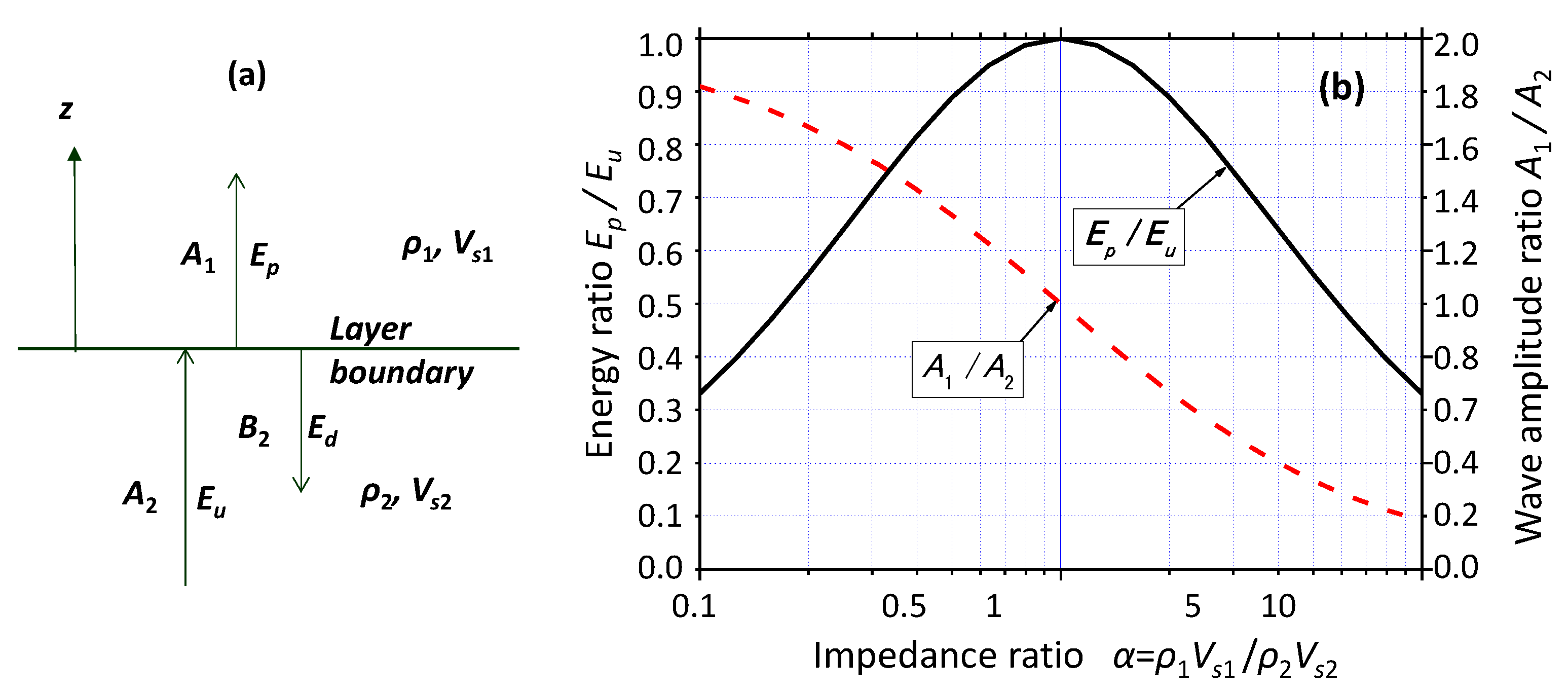
As an example of the energy flow in layered soil deposits under the assumption of one-dimensional propagation of the SH wave, let us first consider infinitely extended media [10] consisting of two parts with an internal boundary as shown in Figure 3a, where z-axis is taken upward from the horizontal boundary. The S-wave velocities are and , and the soil densities are and in the upper and lower parts, respectively. Wave displacements at the upper and lower parts u1, u2 are expressed as:
where ω = the angular frequency and k1 and k2 are the respective wave numbers defined by , . A1 is the amplitude for upward wave in the upper part and A2, B2 are the amplitudes for input upward and reflecting downward waves in the lower part, respectively. The amplitude ratios among A1, A2, B2 can readily be obtained from the boundary condition using the impedance ratio as:
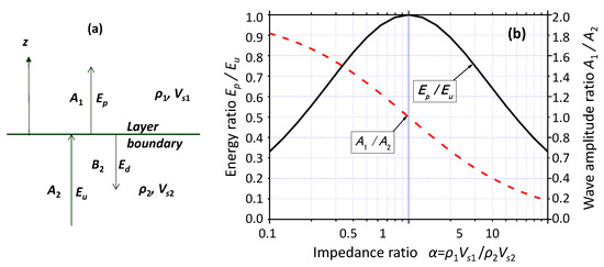
Figure 3.
Energy propagation of upward SH wave through internal boundary in infinite media: one-dimensional model (a) and energy and amplitude ratio in SH wave propagation (b).
Because the energy of the one-directionally propagating SH wave passing through a unit horizontal area is proportional to the square of particle velocity amplitude times associated impedance ratio as defined in Equation (5), the corresponding energy ratios are written as:
where Eu, Ep and Ed are cumulative energies for the upward wave in the lower part, propagating wave in the upper part, and downward wave in the lower part, respectively.
In Figure 3b, the amplitude ratio and the energy ratio of the waves are depicted along the two vertical axes versus the logarithm of impedance ratio in the horizontal axis. Note that the energy ratio Ep/Eu decreases symmetrically as the impedance ratio α is departing from unity, whereas the amplitude ratio A1/A2 monotonically decreases with increasing . This indicates that if a layer boundary exists, the energy Ep always decreases from Eu whether <1 or >1, because a part of the energy in the upward wave is inevitably transferred to the reflecting wave due to the different impedance between the two media.
Such a condition only with upward energy Ep in the upper medium and no downward energy as in Figure 3a may occur not only due to the absence of reflecting upper boundary but also due to complete energy dissipation in the upper part. Hence, the energy ratio Ep/Eu defined in Equation (12) may be interpreted as the upper limit for the input seismic wave energy Eu to be dissipated in an ideal energy absorber wherein all the wave energy transferred can be completely dissipated by earthquake destructions.
2.2. Energy Flow of Harmonic Wave in Two-Layer System
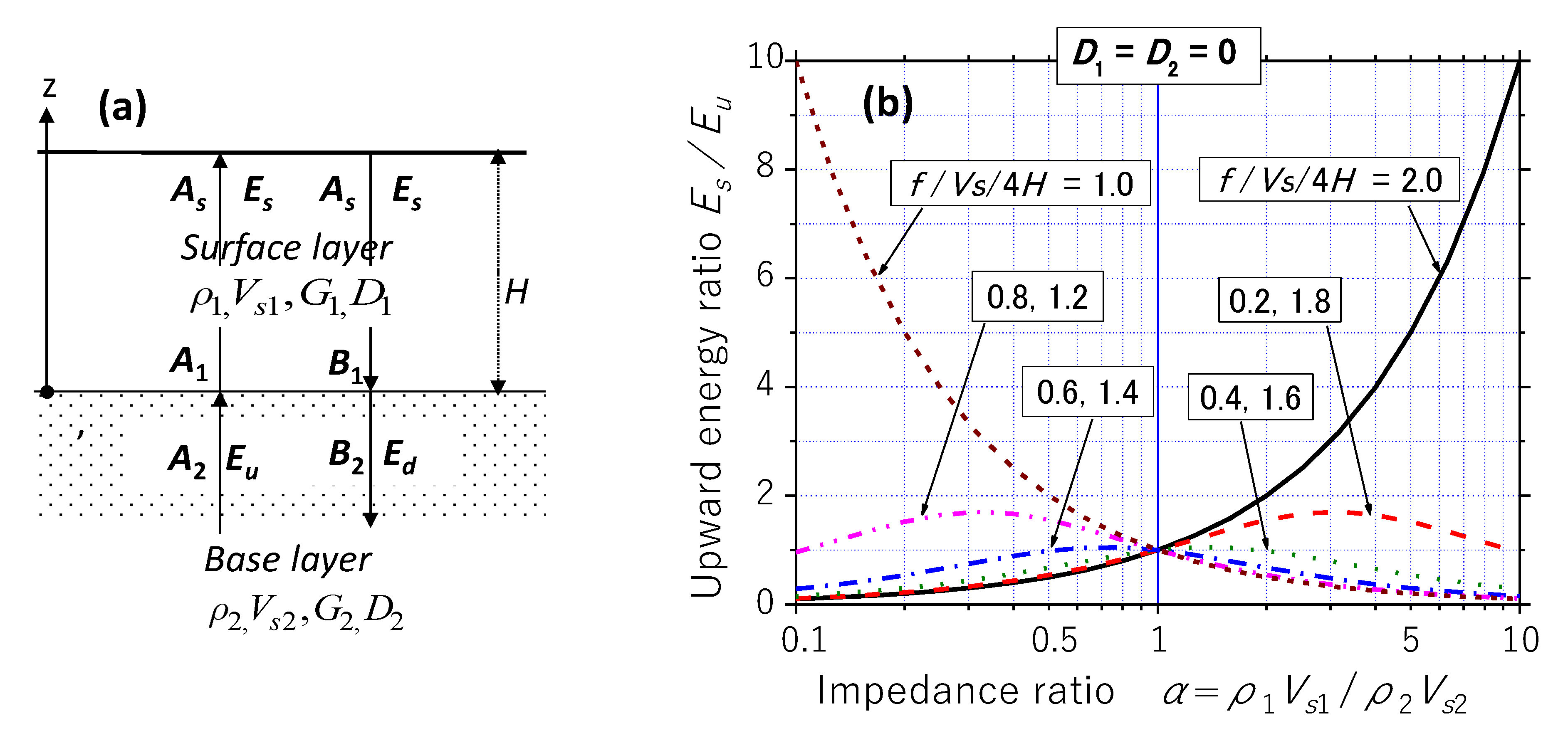
As a next example, the energy flow is considered in the two-layer model shown in Figure 4a consisting of the surface layer of a finite height H underlain by the infinitely thick base layer in stationary response to a harmonic motion [10]. Again, the S-wave velocities are Vs1 and Vs2, and the densities are ρ1 and ρ2, the wave displacements are u1 and u2 in the upper and lower layers, respectively. The horizontal displacement in each layer is expressed using the amplitudes of upward and downward waves A1, B1, in the upper layer, and A2, B2 in the lower layer, respectively as:
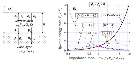
Figure 4.
Two-layer system with harmonic wave propagation (a), and upward energy ratio between surface and base Es/Eu versus impedance ratio α for damping ratio D1 = D2 = 0 (b).
This time, the internal soil damping is considered as D1, D2, in the upper and lower layers, respectively, and hence , are complex S-wave velocity, , are complex wave numbers, and is complex impedance ratio.
Using the displacement amplitudes As at the ground surface correlated with amplitudes A1 and B1 of upward and downward waves at the bottom of the surface layer as:
and considering the boundary conditions at the top and bottom of the layer, the following equations can be readily obtained.
Then, using Equation (6), the ratio of the upward energy at the ground surface Es to that in the base layer Eu is written as:
Likewise, the ratio of corresponding energy flux can be expressed in the same form as Equation (19) as far as the stationary response to harmonic motions is concerned. The ratio between the downward and upward energies Ed to Eu at the top of the base layer is written as:
Furthermore, the ratio of the dissipated energy in the surface layer to the upward energy in the base layer Ew/Eu is expressed as:
because, in the stationary response, the difference between the upward and downward energies at the top of the base layer has to be identical with the energy dissipated in the surface layer as .
Figure 4b depicts the surface energy ratio Es/Eu in Equation (19) for stepwise varying normalized frequencies, f/(Vs/4H), versus the impedance ratio α in the log-scale for zero internal damping (D1 = D2 = 0). The energy ratio varies symmetrically with respect to the center axis = 1.0 where Es/Eu = 1.0 quite reasonably. The maximum energy in the surface layer occurs in the first resonance, f/(Vs/4H) = 1.0, for α < 1.0, whereas it occurs in the second resonance, f/(Vs/4H) = 2.0, for α > 1.0, when Es is much larger than Eu reflecting energy accumulation in the surface layer due to the resonance. By substituting into Equation (19), is obtained as the maximum energy ratio in the first resonance, indicating that the softer the surface soil is, the larger the energy becomes in resonance stored in the surface layer. For off-resonance frequencies such as f/(Vs/4H) ≤ 0.6 or ≥1.4, Es tends to be much lower than Eu with decreasing α for α < 1.0.
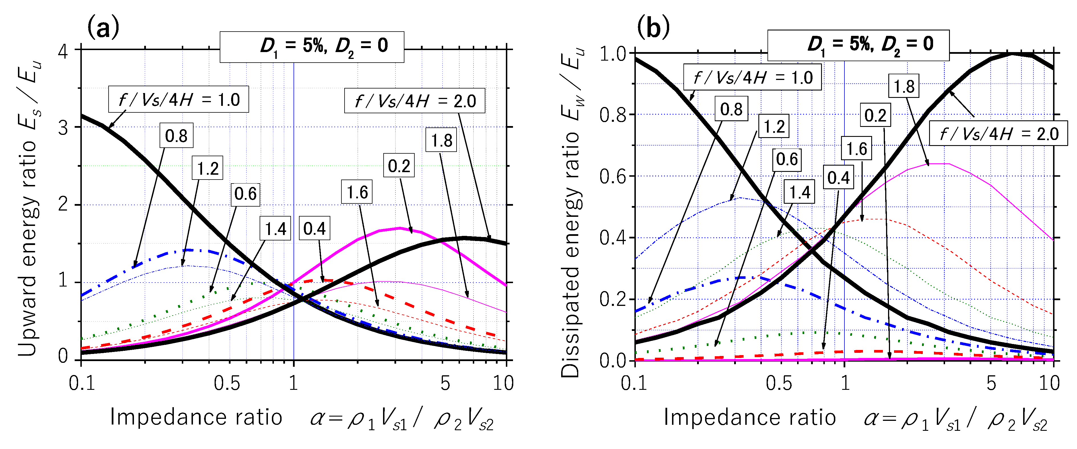
In Figure 5a, the upward energy ratio Es/Eu calculated by Equation (19) for the two-layer model where the internal damping ratio in the surface layer D1 = 5% is depicted versus α. The energy Es tends to decrease evidently compared to the case of D1 = 0%, although the energy accumulation effect near resonance in the surface layer can still be recognized. In Figure 5b, the dissipated energy ratio calculated in Equation (21) for D1 = 5% is shown versus . A considerable energy Ew out of Eu tends to be dissipated rather than stored in and near resonance due to the multi-reflection of the wave trapped in the surface layer.

Figure 5.
Energy flow in two-layer system by harmonic motion with D1 = 5% and D2 = 0%. Surface energy ratio Es/Eu (a) and dissipated energy ratio Ew/Eu (b) versus impedance ratio .
2.3. Energy Flow of Transient Irregular Wave in Two-Layer System
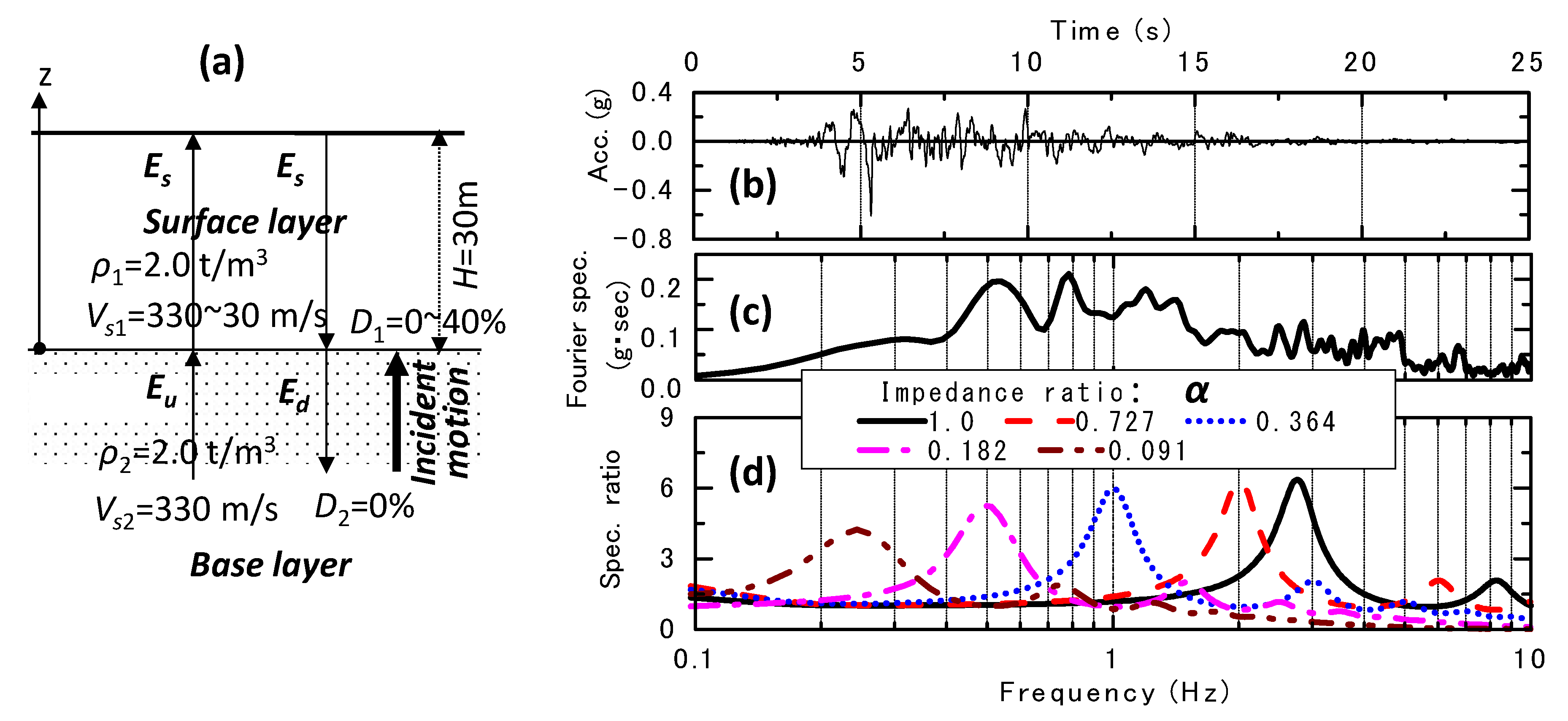
Similar energy flow for a transient irregular seismic wave of a limited duration in the two-layer system in Figure 6a is addressed here [10]. In the surface layer with the thickness H = 30 m and density ρ1 = 2.0 t/m3, S-wave velocity and damping ratio are parametrically varied as Vs1 = 330~30 m/s (impedance ratio α = 1.0~0.091) and D1 = 0~40%, respectively. It is underlain by a base layer with ρ2 = 2.0 t/m3, Vs2 = 330 m/s, D2 = 0%, and the incident wave is given at the top of the base layer. The wave was an incident acceleration motion at GL. −83.4 m in PI (Port Island) vertical array (in the principal direction where maximum acceleration occurred) during the 1995 Kobe earthquake in Japan [16]. Its time–history and Fourier spectrum are depicted in Figure 6b–d, which shows transfer functions between the ground surface and outcropping base layer for α = 1.0~0.091 and D1 = 5%. Note that the two-layer system with α = 0.182 tends to have peak frequencies similar to the input earthquake motion.
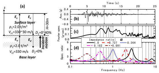
Figure 6.
Energy flow for irregular seismic wave: two-layer model (a), time–history (b), Fourier spectrum (c) of input wave, and transfer functions of two-layer model (d).
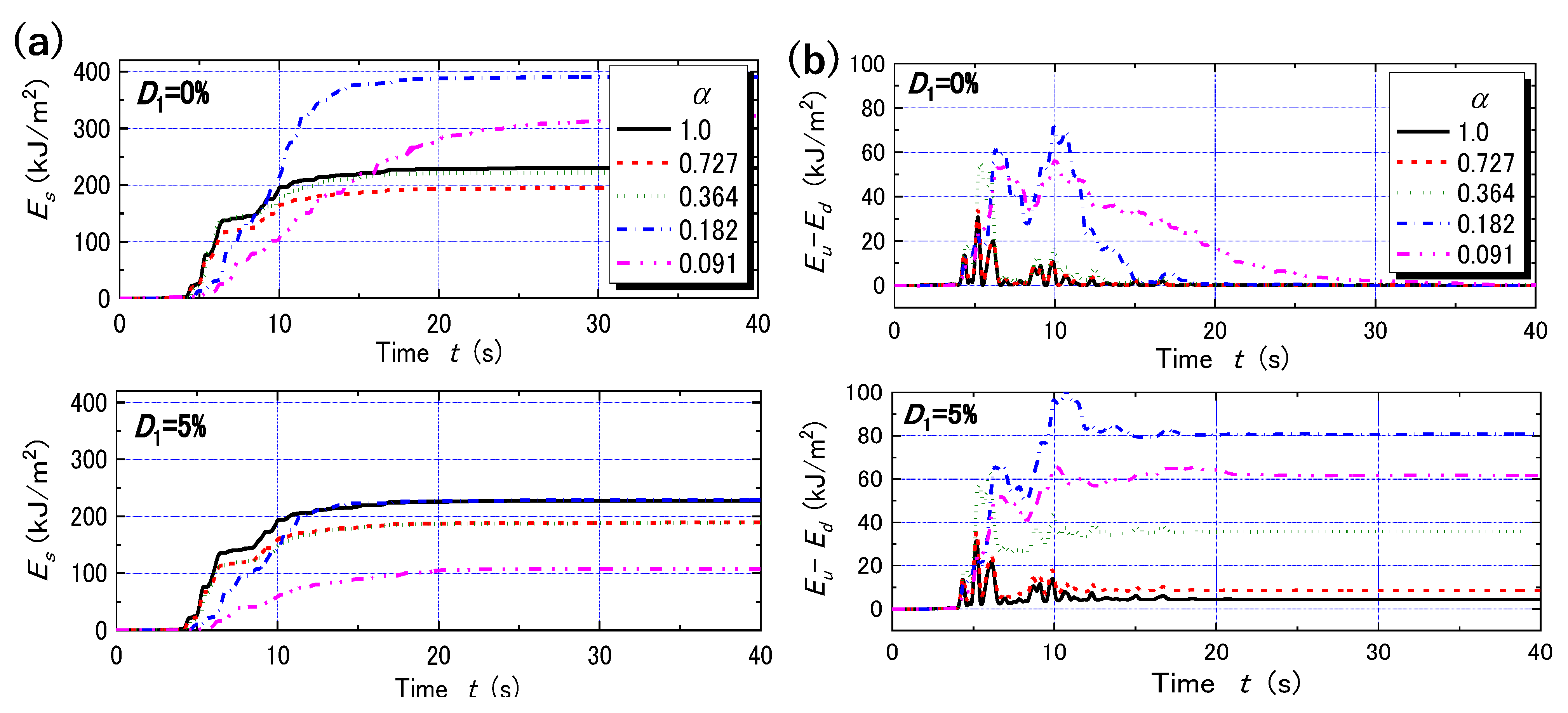
The wave energy E of one-directionally propagating SH wave through a unit horizontal area in a time interval t = t1~t2, and the associated energy flux dE/dt are calculated by Equations (6) and (7) using acceleration response of the two-layer system to the incident motion. Figure 7a depicts the time–histories of wave energy Es at the ground surface for D1 = 0 and 5% in the upper and lower diagrams. The Es value monotonically increases with time to the end of the seismic motion because it is the cumulative energy arriving at the ground surface. Obviously, the ultimate Es value, which may be involved with earthquake damage of structures on the surface, is dependent not only the damping ratio D1 but also on the impedance ratio α. In Figure 7b, the time–histories of the difference between upward and downward energies Eu − Ed in the base layer are depicted in a similar manner. Here, the time-dependent increase and decrease are evidently seen reflecting that the energy stored temporarily in the surface layer eventually returns to the base layer. For D1 = 0, the values Eu − Ed finally return to zero, indicating that no energy dissipation occurs, while for D1 = 5%, they tend to converge to certain non-zero values reflecting the energy loss in the surface layer, which is also dependent on the impedance ratio strongly.
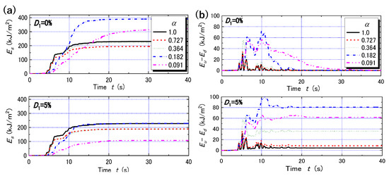
Figure 7.
Time–histories of wave energies for D1 = 0% (top) and 5% (bottom). Upward energy at ground surface Es (a) and energy difference Eu−Ed in base layer (b).
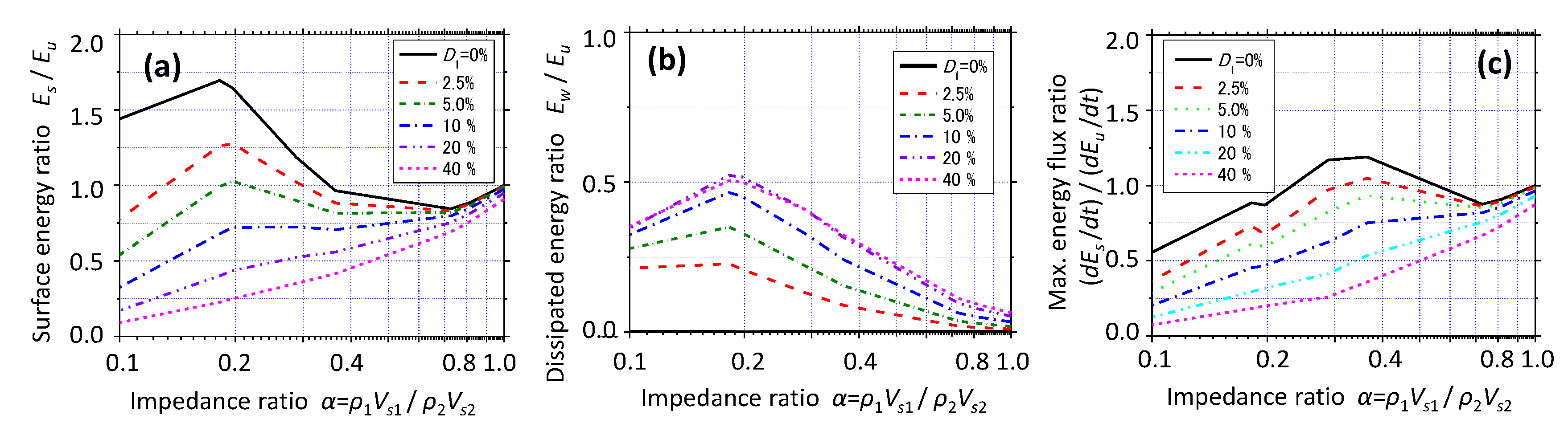
Based on the series of similar calculations for different D1 values, the ratios of surface energy Es to upward energy Eu at the end of the earthquake motion are plotted versus the impedance ratio in Figure 8a. If D1 = 0 or 2.5%, Es/Eu > 1.0 holds for α = 0.182 or nearby, indicating that the energy is temporarily stored in the surface layer because the two-layer system with this α value is in near resonance with the input motion. For D1 > 10%, however, Es/Eu tends to be smaller than unity and decreases monotonically with decreasing α. Figure 8b shows the ratios of dissipated energy Ew = Eu − Ed to Eu at the end of the earthquake motion for different D1 values. Ew/Eu tends to be larger with increasing D1 and takes the maximum at = 0.182 in resonance with the input motion. Thus, the energy storage effect in the surface layer near resonance is cancelled by the increasing dissipated energy Ew with increasing D1 in this model study.

Figure 8.
Energy ratio in two-layer system for irregular seismic motion versus impedance ratio. Surface energy versus base energy Es/Eu (a), dissipated energy versus base energy Ew/Eu (b), max. surface energy flux versus max. base energy flux (dEs/dt)/(dEu/dt) (c).
Apart from the cumulative energy Es shown above, the energy flux defined in Equation (7) is calculated in the surface layer as well as in the base layer, and the ratios of the maximum values (dEs/dt)max/(dEu/dt)max are plotted versus the impedance ratios in Figure 8c. For damping ratio D < 5%, the maximum energy flux takes a peak at an impedance ratio slightly higher than that for Es/Eu in Figure 8a. However, the ratios of energy flux tend to exhibit α-dependent variations similar to those of cumulative energy in that they tend to monotonically decrease with decreasing for D > 10%.
Thus, Figure 8 indicates that during strong earthquakes when a soft surface layer manifests larger damping value, the seismic wave energy Es or the maximum energy flux (dEs/dt)max arriving at the ground surface tends to decrease more relative to Eu or (dEu/dt)max in the base layer with a decrease in impedance ratio. or surface S-wave velocity despite the energy storage effect near resonance in the surface layer, at least for this particular earthquake motion used here. However, this trend can actually be confirmed in a number of vertical array earthquake records as observed in the following.
3. Energy Flow Calculated by Vertical Array Records
Research on the seismic wave energy and energy demand in particular is still limited in number, not only due to historical backgrounds that the energy concept was traditionally not popular as an acceleration in engineering design but also due to difficulties in having subsurface ground motion records. After the 1995 Kobe earthquake, however, more than 700 vertical array strong motion observation stations (KiK-net) were deployed all over Japan, which recorded earthquake motions at downhole depths as well as at the ground surface in the same site for a variety of soil profiles. Here, the subsurface energy flows are calculated utilizing records acquired during nine strong earthquakes that occurred in recent years by assuming the vertical propagation of SH waves to known depth-dependent energy demands and by applying them in engineering design.
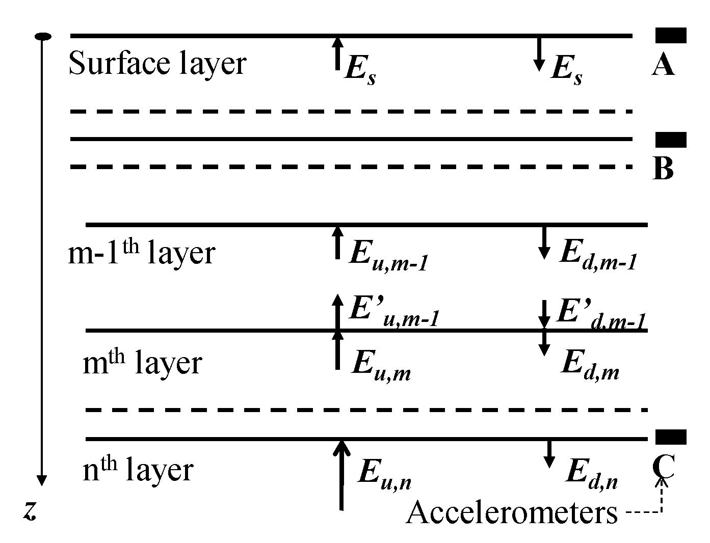
3.1. Energy Flow Calculation Procedure
First, an in situ level ground is idealized by a set of horizontal soil layers where the SH wave propagates vertically as shown in Figure 9. It is essential to separate a measured downhole motion into the upward and downward waves in order to evaluate the energy flow. Let Eu,m, Ed,m, denote the upward and downward energies at the upper boundary of the m-th layer, and corresponding energies at the lower boundary of the (m − 1)-th layer as E′u,m−1, E′d,m−1, respectively. Because of the principle of energy balance at the boundary between the m-th and (m − 1)-th layer
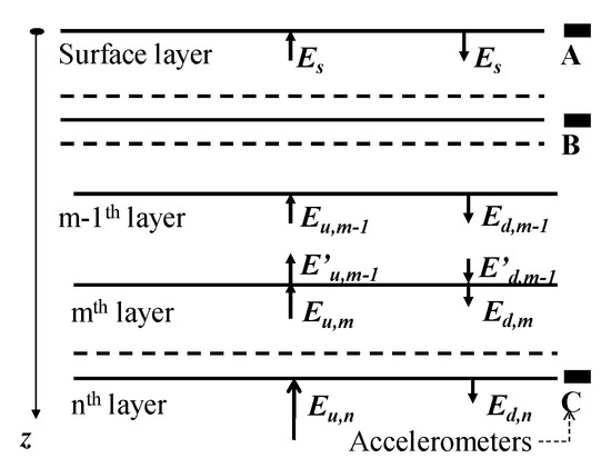
Figure 9.
Level ground idealized by a set of horizontal soil layers with vertical array seismometers.
If the wave energies are evaluated at the end of a given earthquake motion, the energy ET in Equation (22) means the gross energy passing through the boundary during the earthquake. From this, the following equation is readily derived.
Here, Ew stands for the energy dissipated in soil layers above the layer boundary during the earthquake, because all the energy computed here is assumed to transmit vertically.
Based on the multiple reflection theory, the upward and downward SH waves and corresponding wave energies at arbitrary levels can be evaluated from a single record at any level using the condition that the ground surface is free from stress (e.g., Schnabel et al., 1972 [17]). If downhole records are available, however, they will considerably improve the energy flow evaluation, which may not fully comply with the simple theory assumed here. If seismic records are obtained not only at the ground surface (Point A) but also at two subsurface levels, B and C, as illustrated in Figure 9 for example, then the energy flow between B and C can be calculated by using earthquake records at the two levels [9,11]. Between the ground surface (Point A) and Point B, conversely, two sets of energy flow can be calculated using the earthquake record either at A or B. The two sets of energy may then be averaged with the weight of relative proximity to A and B to have the plausible values.
Nine earthquakes (Kobe EQ. and EQ1 to EQ8) and 30 vertical array sites used here are listed in Table 1 with associated parameters. They are of the moment magnitude MW = 6.6 to 7.9 or JMA magnitude MJ = 6.7 to 8.0 (magnitude in Japan Meteorological Agency scale, similar to Richter scale). A total number of 30 vertical array sites was selected for the nine earthquakes with focal distances ranging from 9 to 227 km. The depth of the vertical arrays from the ground surface to the deepest three-dimensional accelerometer spanned from 83 to 260 m, of which most were nearly 100 m. The S-wave velocities at the base were widely diverged as Vs = 380~2800 m/s due to differences in geology, while the surface velocities were mostly Vs = 90~430 m/s. Four vertical array sites for Kobe EQ. and one site for EQ7 consisted of accelerometers at three or more different levels including the ground surface, while all others belonging to the KiK-net consisted of only two levels, surface and base.

Table 1.
Nine strong earthquakes and 30 vertical array sites with associated parameters.
The scalar sum of the wave energies calculated from the two orthogonal horizontal acceleration records were used for the energy flow evaluations. Equivalent linear soil properties S-wave velocity Vs and damping ratio D optimized for main shock records were incorporated in the evaluations, wherein D was assumed as non-viscous or frequency independent (Ishihara 1996 [18]).
3.2. Typical Energy Flows in Two Vertical Array Sites
Typical energy flows calculated are exemplified below in two sites [11]. In Port Island (PI), four accelerometers were installed in soft and deep quaternary deposits, and a strongly nonlinear response during the 1995 Kobe earthquake (MJ = 7.2) was recorded near the causative fault. In Taiki (TKCH08: KiK-net) in Hokkaido, a surface accelerometer on soft-soil surface and a downhole accelerometer in stiff bedrock recorded strong ground motion during the 2003 Tokachi-Oki earthquake (EQ3: MJ = 8.0). Table 2 shows soil profiles and pertinent properties at the two sites.
Table 2.
Soil profiles and properties at two vertical array sites: (a) PI and (b) KiK-net Taiki.
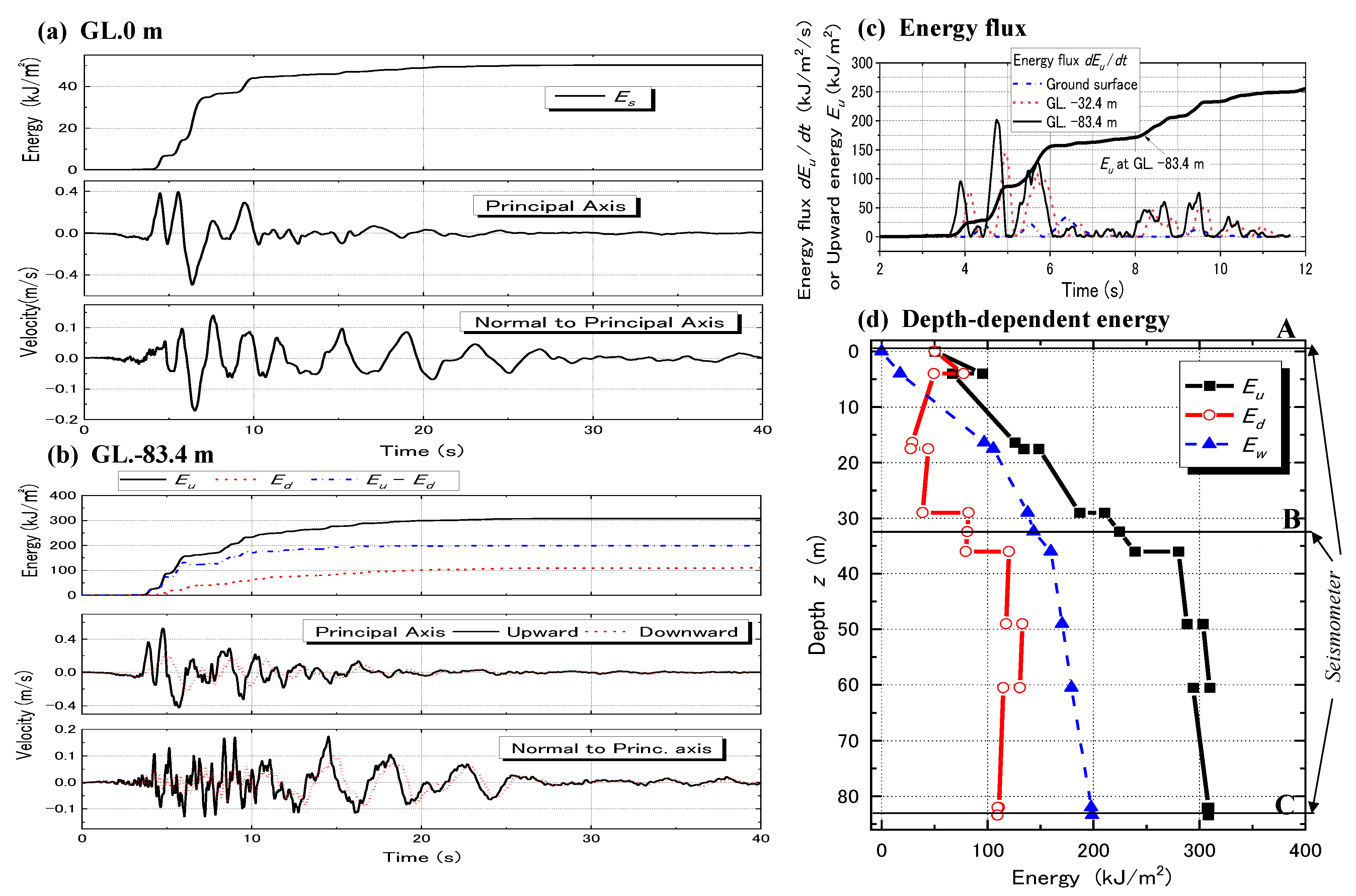
In PI, all the soils are quaternary, and Vs is smaller than 400 m/s even at the deepest level as indicated in Table 2a [11]. Extensive liquefaction occurred in the reclaimed soil down to 17.5 m from the surface [16]. Main shock records at three levels (GL. −0 m, −32.4 m and −83.4 m) were used for the energy evaluation. In the lower two panels of Figure 10a, particle velocity time–histories at the surface (GL. 0 m) are shown in two orthogonal horizontal axes (the principal axis with maximum acceleration and normal to that). In the top panel, the energy at the surface Es as a scalar sum of the two axes calculated from the velocity time–histories and the impedance of the surface layer is shown, where Vs was determined considering the strain-dependent soil nonlinearity [11]. In the lower two panels of Figure 10b, upward and downward velocity waves at the deepest level (GL. −83.4 m) are shown in the two axes. In the top panel, the time–histories of the energies at the deepest level calculated from the velocities are shown. Note that the upward and downward energies, Eu and Ed, show a time-dependent monotonic increase because they are cumulative energies transmitted by one-directionally propagating waves. In contrast, the difference of Eu − Ed indicates the energy balance in the upper soil layers versus the deepest level and hence shows both increase and decrease with time.
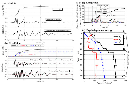
Figure 10.
Calculation of wave energies in PI: time–histories of energy and particle velocity at GL. 0m (a) and at GL. −83.4 m (b), time–histories of depth-dependent energy flux (c), and depth-dependent cumulative energies Eu, Ed and Ew (d).
In Figure 10c, the corresponding energy fluxes of upward waves dEu/dt calculated in Equation (7) are depicted at three depths (GL. −0, −32.4 and −83.4 m) [11]. Different from the cumulative upward energy Es or Eu, the energy flux tends to significantly fluctuate versus elapsed time with several peaks. As exemplified at GL. −83.4 m, these peaks in dEu/dt are obviously synchronized with the sections of higher time gradient of Eu in the thick curve. This indicates that the energy flux is dependent on wave forms of particular earthquake motions. The energy flux dEu/dt tends to decrease with decreasing depths, similar to the energy Eu.
Figure 10d shows the distributions of the energies Eu, Ed, Ew in PI along the depth at the end of the earthquake record. The energies between B and C are uniquely determined from the combination of records at B and C based on the multi-reflection theory [11]. In contrast, either the record A at the surface or B is sufficient to calculate the energies between A and B, wherein the free surface boundary condition is utilized. In PI, where strong soil nonlinearity due to extensive liquefaction occurred in the surface layers, record B was exclusively used for the energy calculation between A and B because it was likely to be less influenced than record A by liquefaction-induced nonlinearity that was difficult to evaluate reliably. Record A was used for computing the energy at A only, which was 50 kJ/m2 in contrast to 86 kJ/m2 calculated from record B. The energies at B obtained from the combination of record B and C were Eu = 236 kJ/m2 and Ed = 80 kJ/m2, whereas those from record B together with the free surface condition were Eu = 212 kJ/m2 and Ed = 82 kJ/m2, respectively. Although the differences were not large, the energies Eu and Ed at the intermediate depths were averaged as already mentioned. In order to avoid discontinuous depth-dependent variation near the intermediate point B in Ew, the following modifications in Equation (24) were implemented.
Figure 10d shows an obvious decreasing trend of Eu from the deepest level to the surface, particularly in the top 36 m. The downward energy Ed is evidently smaller in the top 36 m than in the deeper part. As a result, the dissipated energy Ew = Eu − Ed tends to increase considerably with increasing depth. The increasing rate of Ew from the surface down to 17.5 m deep in the liquefied layer is particularly large, quantifying that the energy loss per unit volume in the liquefied soil was 6 kJ/m3 on average.
In laboratory liquefaction tests on soils sampled in this site, the cyclic resistance ratio for liquefaction in the number of cycles = 15 was found as CRR15 = 0.24 (Inagaki et al., 1996 [19]). The cumulative dissipated energy corresponding to CRR15 = 0.24 can be read off from an empirical formula developed by a number of tests on in situ soils as = 0.061 according to Kokusho and Tanimoto (2021) [20]. Because the effective confining stress in the liquefied layer of GL. −3.5~17.5 m is approximated as 100 kPa on average, the cumulative dissipated energy is obtained as 6.1 kJ/m3, showing good coincidence with the above-mentioned value quantified from in situ wave propagation.
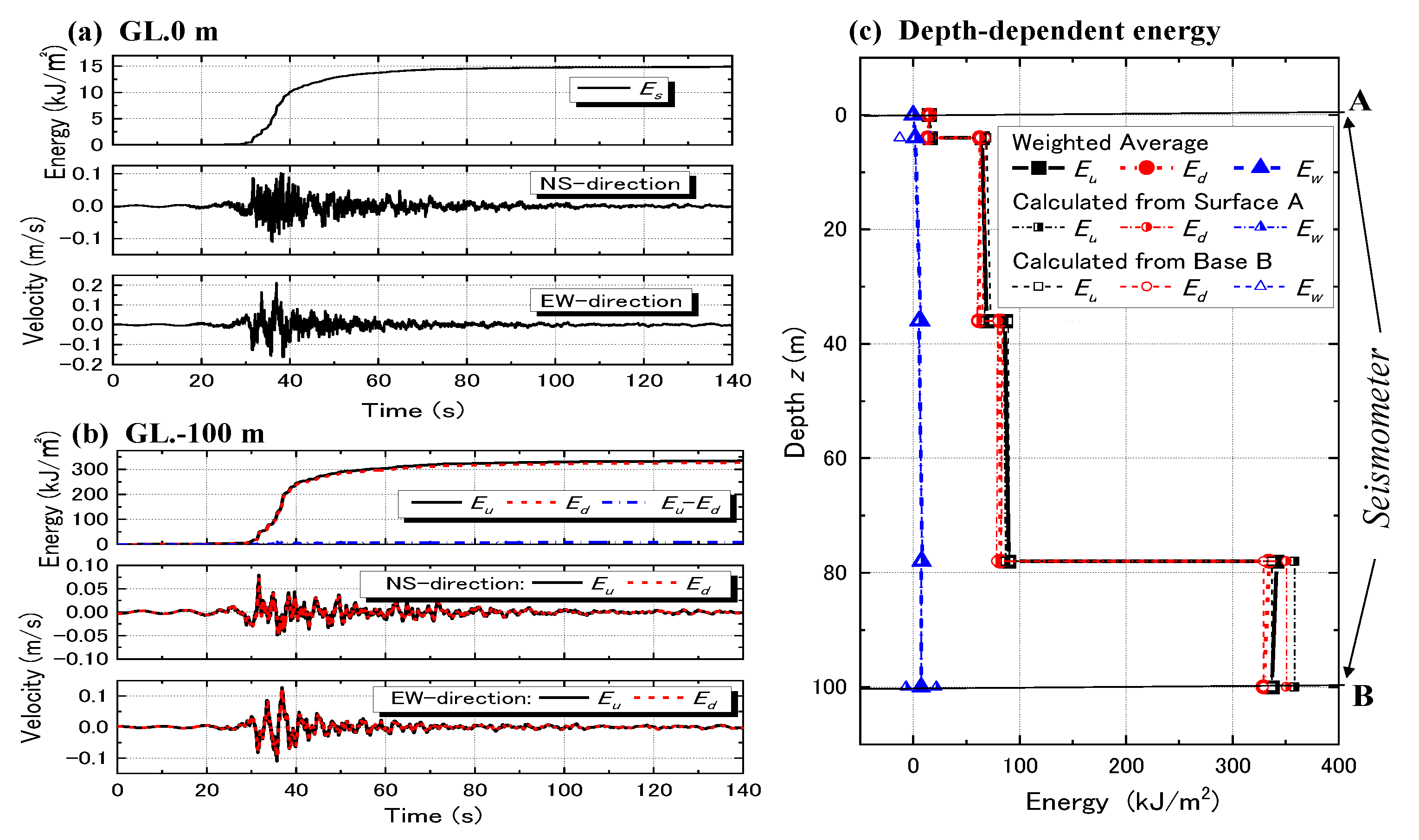
Table 2(b) shows profiles and soil properties at one of the KiK-net sites, Taiki (TKCH08). Quite different from PI, the bedrock is stiff (Vs = 2800 m/s) at the deepest level (GL. −100 m), while the small-strain Vs in the surface layer is as low as Vs = 130 m, which further degraded during the main shock. Main shock records of EQ3 in two horizontal directions at the surface (record A) and the deepest level at GL. −100 m (record B) were used for the energy flow calculation [11].
In the lower two panels of Figure 11a, particle velocity time–histories at the surface (GL. 0 m), calculated from record A are shown in NS and EW directions, while in the top panel, the upward energy at the surface calculated from them is shown as the sum in the two orthogonal directions. In Figure 11b, velocity time–histories of upward and downward waves at the deepest level of GL. −100 m calculated from record B in the two directions and the energy time–histories at the same level are shown in the same manner. Both upward and downward energies, Eu and Ed, show rapid increase with a marginal difference to each other, resulting in a small value of , indicating that energy dissipation in this site is small, reflecting the stiff soil condition, except for in the top layer.

Figure 11.
Calculation of wave energies in KiK-net Taiki: time–histories of energy and velocity at GL. 0 m (a) and at GL. −100 m (b) and depth-dependent cumulative energies Eu, Ed and Ew (c).
In Figure 11c, the energy flows along the depth calculated either from record A at surface or from record B at base are plotted with different symbols. The thick lines with close symbols are the average of the two calculations with the weight of the relative proximity to levels A and B. The two energy flows calculated from A and B are similar to each other, indicating that the soil model is a good reproduction of the actual ground at this particular site. Thus, the averaging procedure tends to modify the depth-dependent energy variations to a certain degree, while the energy values at the base and at the surface are free from this modification.
In the Taiki-site, with an upward energy of more than 300 kJ/m2 at the deepest level, less than 100 kJ/m2 passed through the boundary (GL. −78 m) of the drastic impedance change, and only 15 kJ/m2 reached the ground surface, indicating a considerable decrease in upward energy with decreasing depth here again. A small difference between Eu and Ed indicates that the considerable upward energy was reflected at the intermediate boundaries and returned to the deeper ground as the downward energy, without arriving to the soft soil layer near the surface. This also means that the dissipated energy Ew could not be large because most of the upward energy reflected without dissipation before arriving at the soft layers.
3.3. General Trends of Energy Flow Observed in Vertical Arrays
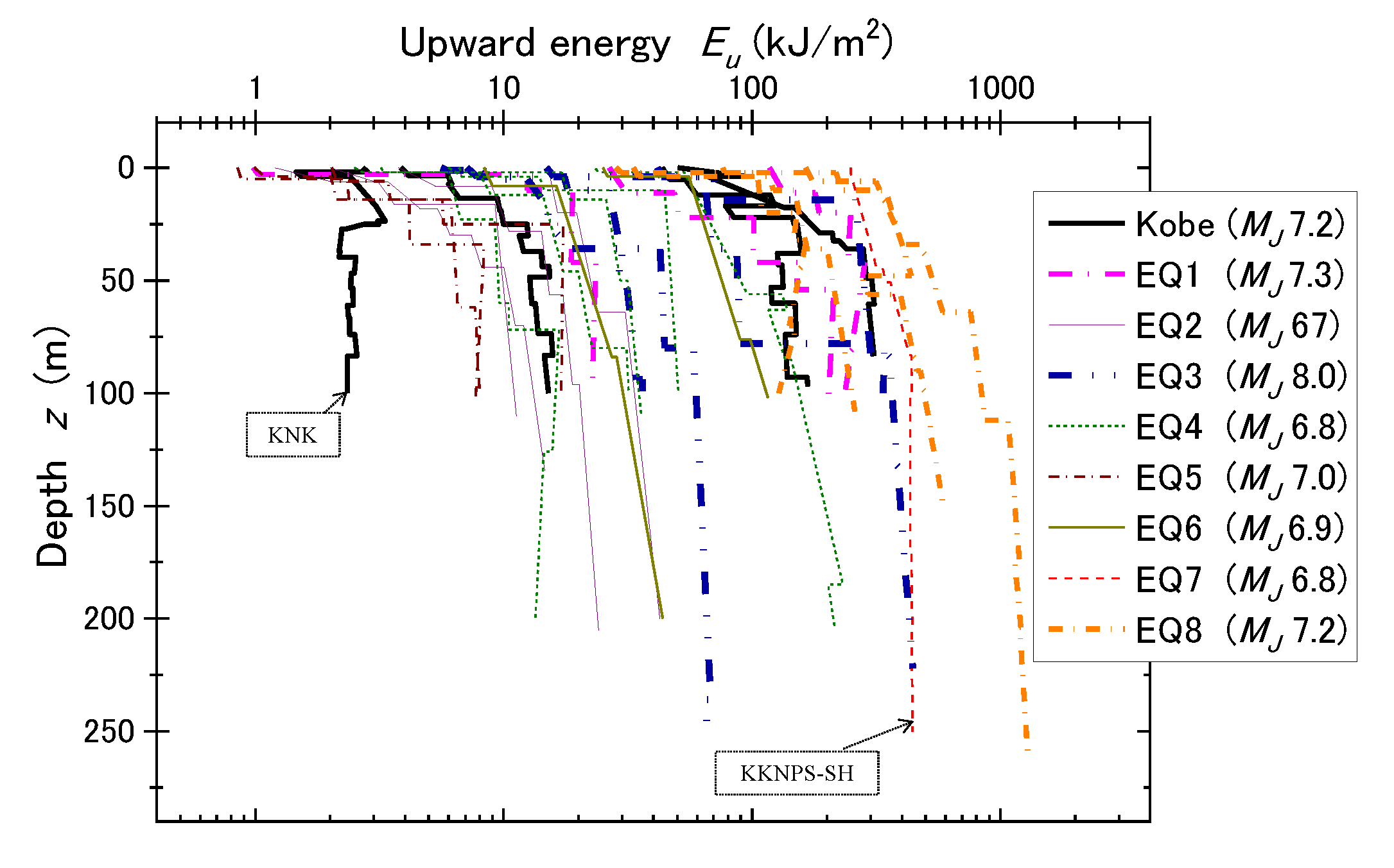
Figure 12 depicts the variations of upward energy Eu along the depth z calculated for nine earthquakes at 30 vertical array sites in the same manner as above [11]. On account of large differences in absolute energy value among the earthquakes, the horizontal axis is taken in logarithm. As PI and Taiki explained above, the upward energies show obvious decreasing trends in most sites with decreasing depth, irrespective of the differences in the absolute upward energy. In some sites, the Eu value decreases to less than one-tenth from the base to the surface. The decreasing trend is more pronounced near the surface in contrast to the depth of 50~100 m or below.
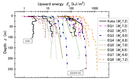
Figure 12.
Variations of upward energy Eu along depth calculated for nine earthquakes at 30 vertical array sites.
There exists a traditional view in engineering seismology (Joyner and Fumal 1984 [21]) that the wave energy (=square of velocity amplitude × wave impedance) is kept constant as seismic waves propagate underground. Hence, the velocity amplitude was generally considered inversely proportional to the square root of the impedance . Figure 12 indicates that this may not be true at least in shallow depth, although there is a small number of exceptional cases, KKNPS-SH and KNK sites, indicated in the chart, wherein the energy tends to be almost constant or decreasing mildly toward the ground surface.
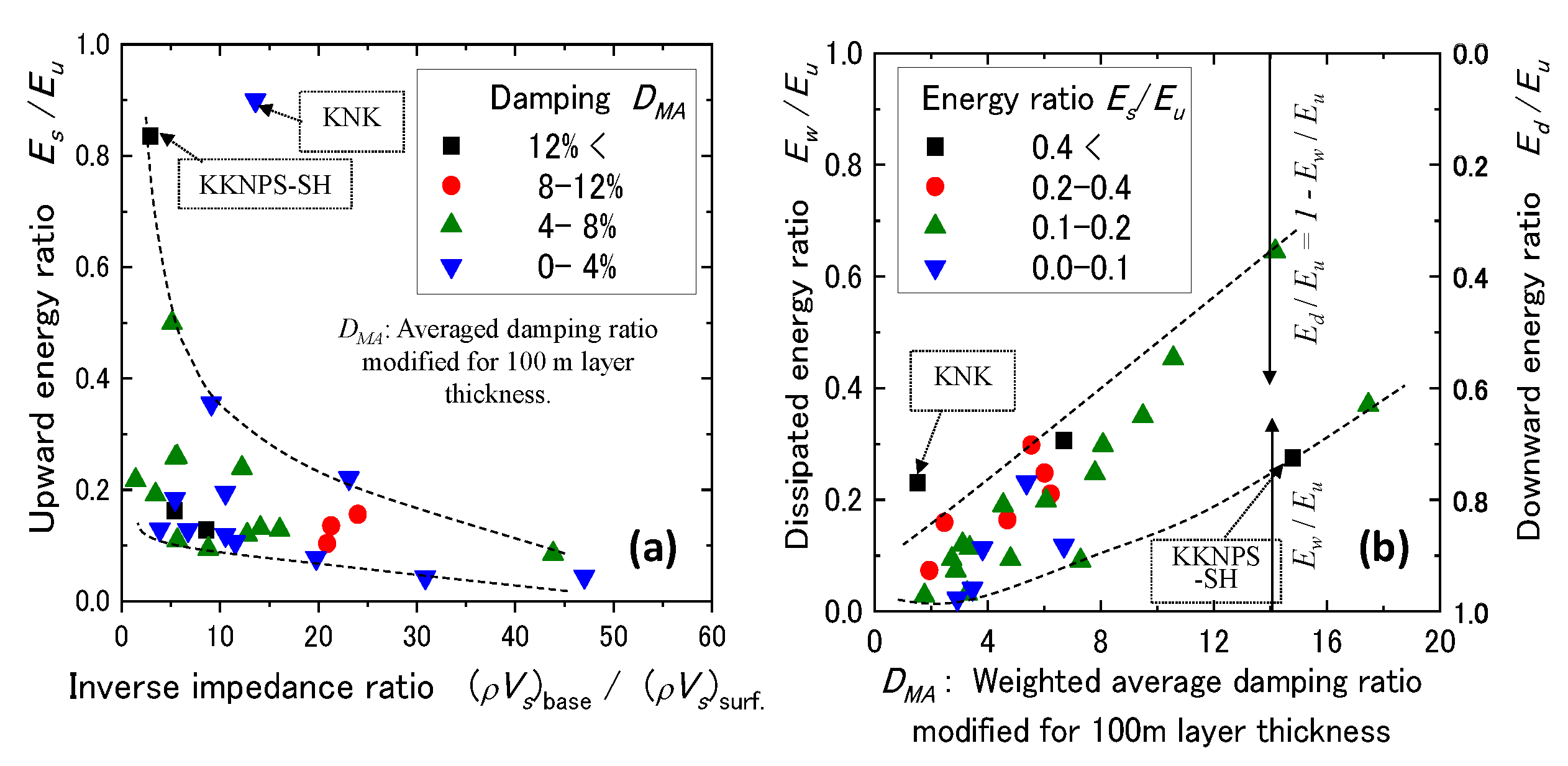
In order to examine how the energy decreasing trend is influenced by site conditions including those exceptional cases, Figure 13a shows ratios of upward energies between surface and base, Es/Eu, plotted versus corresponding inverse impedance ratios [11]. From the data points between the two dashed boundary curves, it may be recognized that the energy ratio Es/Eu tends to decrease with increasing ratio despite data dispersions. The data point for KKNPS-SH may be compatible with global trends in this chart, although for KNK, it is still difficult to explain. From this chart, the upward energy at ground surface tends to be smaller relative to that at base layer in soft soil sites with smaller impedance than in stiff soil sites in accordance with the basic studies in the two-layer system already addressed. Out of 30 sites, the energy ratio Es/Eu > 0.3 holds in only four sites, including KKNPS-SH and KNK. In all the other sites, only less than 10% to 30% of the upward energy at the deepest level arrived at the surface.
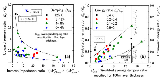
Figure 13.
Upward energy ratio between surface and base (Es/Eu) plotted versus inverse impedance ratios (ρVs)base/(ρVs)surface for all sites (a) and ratios of dissipated energy to upward energy at deepest level Ew/Eu versus modified average damping ratio DMA for all sites (b).
It may well be expected that not only the impedance ratio as mentioned above but also the damping ratios of the individual sites may affect the energy ratio Es/Eu. Hence, the plots are differentiated with four symbols in Figure 13a according to four steps of DMA, modified average damping ratios normalized for the ground thickness 100 m [11]. This chart however does not seem to show the effect of the damping ratio as obviously as that of the impedance ratio.
In Figure 13b, the ratios of the dissipated energy to the upward energy Ew/Eu calculated at the deepest levels of the vertical arrays are taken in the vertical axis versus the modified average damping ratios DMA in the horizontal axis. It reveals that, in most sites, the dissipated energy cannot be more than 30% to 40% of the upward energy. Despite the large data scatters, the plots are in between a pair of dashed curves shown in the diagram, indicating that the energy ratio Ew/Eu tends to increase with increasing damping ratio DMA. The plots are classified into four steps of the upward energy ratio Es/Eu with different symbols. A trend can be observed that the plots with higher Es/Eu tend to be located at higher positions on the chart despite a few exceptions, suggesting that the more energy that reaches the ground surface, the larger the energy loss that can occur presumably in the shallow ground.
It is readily understood from Equation (23) that the downward energy normalized by the upward energy is expressed as , meaning that the vertical axis in Figure 13b can represent Ed/Eu as in the right vertical axis of the diagram. Hence, in most sites during strong earthquakes, Ed/Eu > 0.6~0.7 and more than 60% to 70% of the upward energy at the deepest level goes back to the deeper ground without being dissipated in the upper ground. If Es/Eu < 0.1~0.3 in most sites in Figure 13a mentioned above is reminded, the major mechanism to make the surface energy ratio low is not the energy dissipation in soils because the energy ratio Ew/Eu < 0.3~0.4 is not large enough to account for it. Instead, it is largely attributed to wave reflections at intermediate layer boundaries that interrupt the energy going up such that only a small portion of the upward energy at the base can arrive at the ground surface, particularly in softer soil sites.
4. Empirical Formulas for Upward Energy
4.1. Correlation of Upward Energy Ratio with Impedance Ratio
In order to evaluate how the upward wave energy tends to decrease as it approaches the ground surface, an empirical formula was developed, wherein ratios of upward energies between layers are correlated to corresponding impedance ratios using the dataset of vertical array records addressed above [12]. Out of the depth-dependent upward energy variations at 29 sites excluding the abnormal KNK-site, 23 sites were used, wherein the difference in the two upward energies at the deepest level calculated from measured motions at the ground surface and the deepest level were within about 25%.
Impedance ratios and upward energy ratios β defined between two neighboring layers, m and m + 1, in a given soil profile were calculated individually from surface to base as:
The soil density ρ was assumed depending on the S-wave velocity as: 1.6~2.0 t/m3 for Vs ≤ 300 m/s, 2.0~2.2 t/m3 for 300 m/s ≤ Vs ≤ 700 m/s, 2.3~2.4 t/m3 for 700 m/s ≤ Vs ≤ 1000 m/s, and 2.5~2.7 t/m3 for 1000 m/s ≤ Vs < 3000 m/s. The energy ratios β are plotted versus the corresponding impedance ratios α in Figure 14a for all layers above the deepest levels with different symbols in the 23 vertical array sites. For the majority of the data points, α ≤ 1.0 holds because the impedance ratio is normally less than unity ( is getting larger in deeper layers). It is quite reasonable to assume that β = 0 for α = 0, and β = 1 for α = 1 (equivalent to a uniform ground). Hence, a simple power function may be practically used for 0 ≤ α ≤ 1.0 to approximate the plots as the thick solid curve shown in Figure 14a, and the power n = 0.70 is obtained from the least mean square method with the determination coefficient R2 = 0.81.
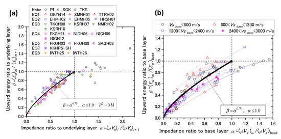
Figure 14.
Upward energy ratios β versus corresponding impedance ratios α compared with empirical formula: between neighboring layers (a) and between a given layer and base layer (b).
Furthermore, the impedance ratio α and the upward energy ratio β may be redefined as different from Equation (25), between an arbitrary layer m (m = 1 to n − 1 in a given soil profile consisting of n-layers) and the deepest layer (n-th base layer) in vertical arrays as follows.
Here, and are the upward energy and seismic impedance in the base layer, respectively. In Figure 14b, data points for all the layers at the 23 vertical array sites are plotted on the α-β diagram, wherein the symbols are connected with thin dashed lines for individual sites and differentiated according to four classes of Vs value at the base layer. Although the plots are more dispersed than in Figure 14a, the superposed curve by Equation (26), using α and β redefined in Equation (27) seems to fairly represent the plots. The base layers in the chart involve those with Vs as high as 2400–3000 m/s, which is almost equivalent to the seismologically defined bedrock. This indicates that it may be possible from a practical point of view to use Equation (26) in order to evaluate the upward energy in a shallow soil layer from that at a base layer having a variety of Vs by considering the impedance ratio between the two corresponding layers.
4.2. Upward Energy at Vertical Array Base and Seismological Bedrock
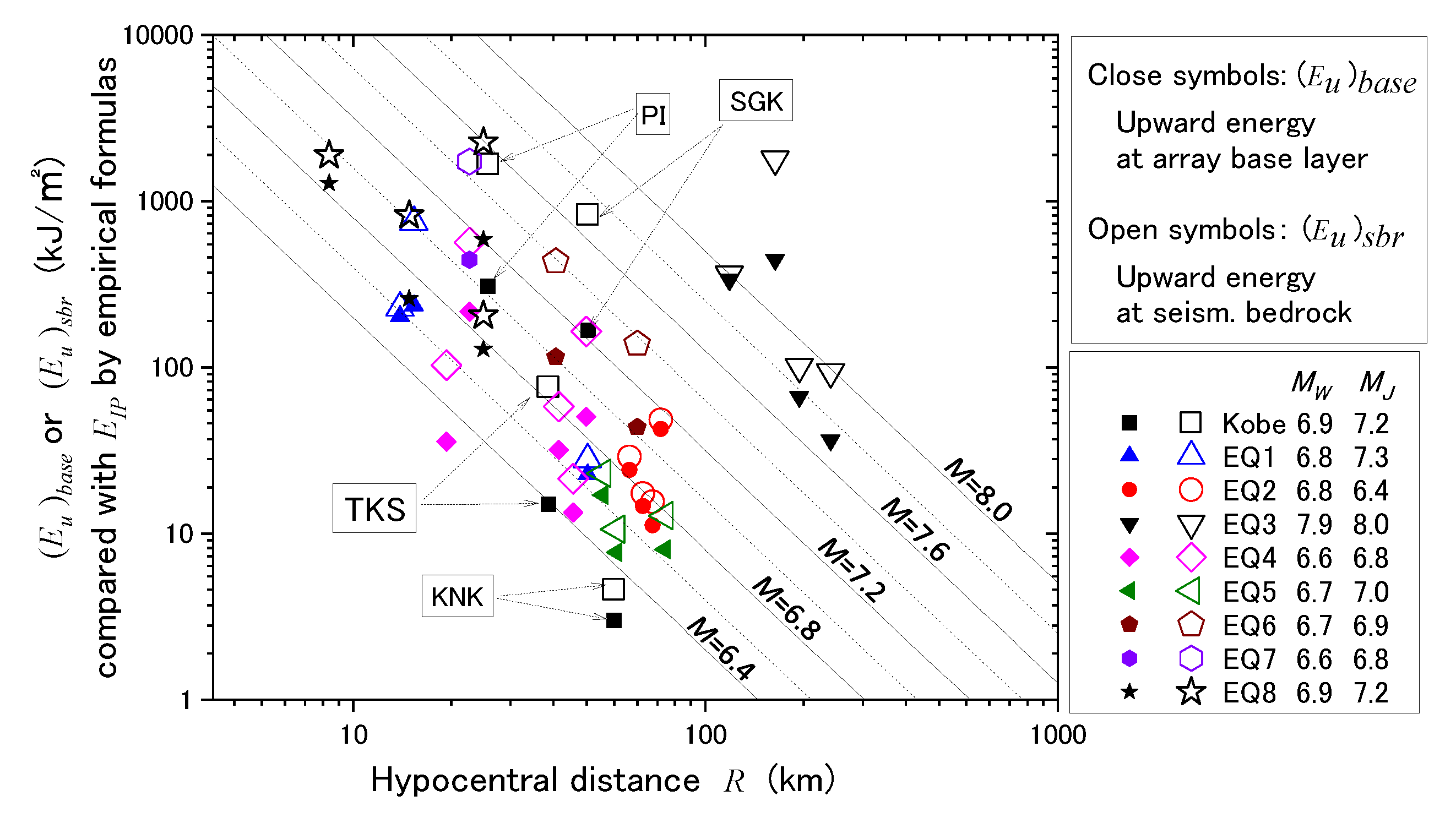
Upward energies at the deepest levels (base layer) are denoted here as (Eu)base calculated from the upward waves (obtained by the multi-reflection analyses using the observed downhole records), and the associated impedance values are plotted in the full-logarithmic scale versus hypocenter distances R in Figure 15 at all 30 vertical array sites with various close symbols corresponding to nine earthquakes [12]. Although the plots are widely dispersed, the decreasing trends in (Eu)base with increasing R for individual earthquakes are recognizable. Among the nine earthquakes, the plots of EQ3 with MJ = 8.0 (2003 Tokachi-Oki earthquake) are reasonably located relatively higher on the upper-right side of the diagram, while others with MJ around seven are lower on the lower-left side.
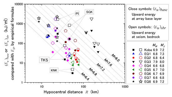
Figure 15.
Upward energies at array base (Eu)base or seismological bedrock (Eu)sbr versus hypocenter distance R, compared with incident energies EIP versus R lines by empirical formulas.
Based on the finding that Equation (26) may be conveniently used to roughly evaluate the energy ratio between arbitrary two layers, the same equation was further used here to estimate the upward energies at the seismological bedrock (Eu)sbr from those at the base layer (Eu)base of the individual vertical arrays. It may well be justified here that major wave energy is still carried by vertically propagating SH wave, even in stiff rocks, down to the seismological bedrock despite potentially increasing involvement of SV waves. The impedance for the seismological bedrock is postulated here as Vs = 3000 m/s and ρ = 2.7 t/m3. In Figure 15, the energies at the seismological bedrock (Eu)sbr thus calculated are superposed with open symbols for the nine earthquakes. They are all positioned higher than the corresponding close plots because of a higher value than that at the bottom of the vertical array, indicating that the upward energy carried presumably by the SH wave tends to reduce as it travels from the seismological bedrock to the engineering bedrock.
Straight dashed lines shown in Figure 15 represent the following formula in terms of incident energy EIP (kJ/m2) taken in the vertical axis versus hypocenter distance R (m) by assuming the spherical energy radiation of body waves from the center of energy release, assumed here as the hypocenter (e.g., [4,5]).
Total released wave energy ETotal in kJ is calculated by the next empirical formula [6] often used in earthquake engineering calculated from earthquake magnitudes M.
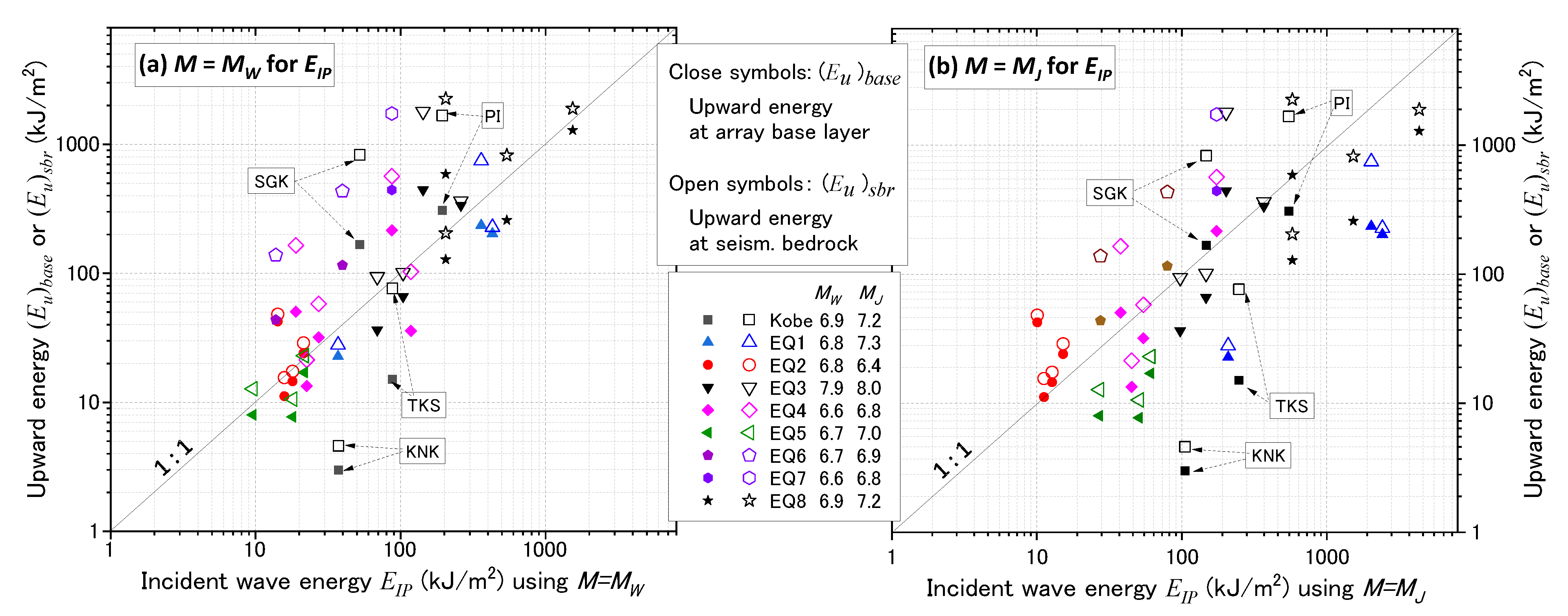
In Figure 16, the energies (Eu)base and (Eu)sbr at the 30 vertical array sites are directly plotted in the vertical axis to compare with the incident energies per unit area EIP, calculated by Equations (28) and (29) in the horizontal axis for individual earthquakes on a log-log diagram. Note that the magnitude M in Equation (29) is represented by MW (Moment magnitude) in Figure 16a versus MJ (JMA magnitude) in Figure 16b. It is recognized that a larger number of plots are located near the diagonal 1:1 line in Figure 16a,b, indicating a basic compatibility between the wave energies determined from vertical array data and the well-known empirical formulas, although the plots are considerably scattered individually.

Figure 16.
Upward energies (Eu)base at engineering bedrock and (Eu)sbr at seismological bedrock versus empirically formulated incident energy EIP by using earthquake magnitude as M = MW (a) and M = MJ (b).
The large scattering may well be expected because such simple formulas as Equations (28) and (29) cannot make good energy predictions, wherein pertinent earthquake fault parameters, such as fault type, fault dimension, directivity, asperity, etc. are completely neglected. For example, the PI and SGK sites during the 1995 Kobe earthquake in Figure 16 largely overshoot the empirical EIP values both in (a) and (b). Forward directivity effect may possibly have been exhibited, making the energy in these sites extraordinarily large in contrast to TKS and KNK, which were perpendicular to the direction of directivity during the same earthquake (Somerville 1996 [22]).
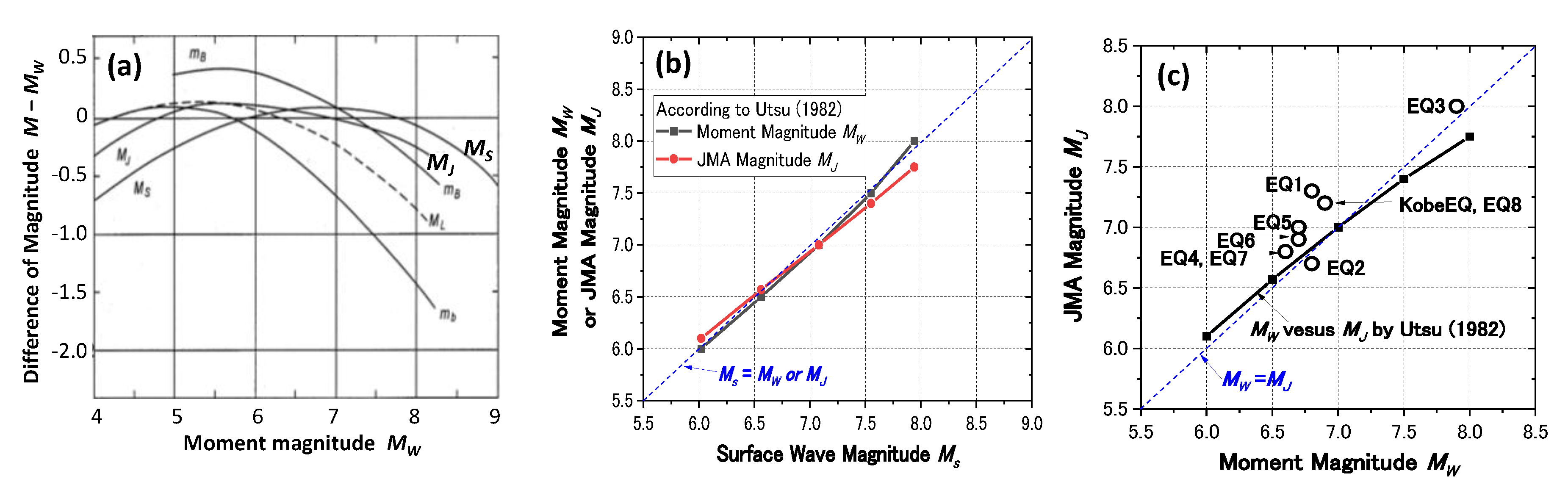
With regard to the difference between Figure 16a,b, it should be reminded that in the original paper by Gutenberg [6] the surface wave magnitude MS was employed as M in Equation (29). A chart on mutual relationships among different earthquake magnitudes was developed by Utsu (1982) [23] as indicated in Figure 17a. According to that chart, MS may be similar to Moment Magnitude MW and Japanese Meteorological Agency Magnitude MJ as well with a small difference of less than 0.2 for MW = 6.0~8.0 as depicted in Figure 17b. Hence, the direct relationship between MW and MJ can be plotted near the dashed diagonal line MW = MJ in Figure 17c according to the relationships in Figure 17a. However, the actual magnitude values of the nine earthquakes (Kobe EQ, EQ1~EQ8) overlaid in Figure 17c reveal that MW < MJ mostly. These individual magnitude values were announced by several agencies such as JMA in Japan and USGS in the USA, and they are essentially coincidental with little difference.
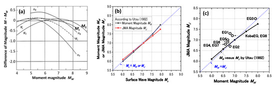
Figure 17.
Mutual relationships among different magnitudes: relationships among various magnitudes modified from Utsu 1982 [23] (a). Relationship between Surface Wave Magnitude Ms versus Moment Magnitude MW or JMA Magnitude MJ [23] (b). Direct relationship between MW and MJ [23] compared with the magnitudes announced for the nine earthquakes (c).
Consequently, the incident wave energy estimated by the empirical formula Equations (28) and (29) using M = MJ tend to be more compatible than M = MW with the upward energies (Eu)sbr at the seismological bedrock (open symbols) in Figure 16b, while in Figure 16a, the empirical formula tends to underestimate the (Eu)sbr values. Thus, the JMA magnitude may be suitable to estimate the incident energy EIP at the seismological bedrock, although crudely for engineering purposes, and more detailed studies will be needed for the empirical equations to be upgraded by incorporating fault and path mechanisms of individual earthquakes.
5. Seismic Design Considerations in View of Energy
Energy-based design considering earthquake wave energy as a demand has rarely been employed in engineering practice compared to force-based design using acceleration or seismic coefficients. Nevertheless, the energy-based design seems to have a great advantage over the force-based design in view of the uniqueness of energy capacity in failure, irrespective of differences in dynamic loading history. It is typically shown in such a problem, such as in soil liquefaction in particular, as demonstrated by Towhata and Ishihara (1985) [24], Yanagisawa and Sugano (1994) [25], Figueroa et al., (1994) [26], Kokusho (2013) [27], Kokusho and Kaneko (2018) [28], and many others. All have recognized that dissipated energy almost uniquely determines pore–pressure buildup ratio and induced strain in cyclic loading of sands almost irrespective of the loading histories, demonstrating the uniqueness of energy capacity. Green et al. (2000) [29] proposed an energy-based pore–pressure generation model, showing that it can approximate test results on sand and silt–sand mixtures at various densities.
Energy-based evaluation methods (EBM) for soil liquefaction comparing energy demand with the energy capacity were proposed by Davis and Berrill (1982) [8], followed by Law et al. (1990) [30], where the demand was given by empirical formulas similar to Equations (28) and (29). In a different approach, Kayen and Mitchell (1997) [31] used Arias Intensity [32] as a demand for the assessment of liquefaction potential, although the Arias Intensity is physically different from the energy because the soil impedance is absent there.
Kokusho (2013) [27] and Kokusho and Mimori (2015) [33] have proposed EBMs where depth-dependent energy demand such as in Figure 12 is compared with energy capacity to determine liquefaction potential layer by layer without using acceleration motions, by introducing a simplification on the ratio of strain energy to total wave energy near ground surface (Kokusho 2017) [34]. Besides these, the base-isolation mechanism of upward wave energy caused by soil liquefaction has also been investigated from the viewpoint of energy demand (Kokusho 2014) [35]. Furthermore, Kokusho 2020 [36] has developed simplified evaluation steps to predict not only liquefaction potential but also induced strain and soil surface settlement by assuming equal allocation of the energy demand to potentially liquefiable layers. One of the excellent features of the EBM was pointed out there that energy demand available is allocated among multiple liquefiable layers to compare with corresponding energy capacity, while in conventional stress-based liquefaction, no evaluations paid attention to acceleration demands of other liquefiable layers.
The energy demand has also been employed to evaluate seismically induced slope failures by comparing them with gravity energy in downslope sliding and frictional energy dissipating in sliding debris (Kokusho and Ishizawa 2007 [37]). The EBM for slope evaluation was applied to cases of earthquake-induced slope failures to back-calculate mobilized friction coefficients during devastating earthquakes in Japan (Kokusho et al., 2011 [38], 2014 [39]). Furthermore, an energy-based Newmark-type evaluation has been developed, wherein the energy demand can almost uniquely evaluate slope displacement in a similar physical model of slope sliding as the Newmark model (Newmark 1965 [40]) without computing displacements using design acceleration motions (Kokusho 2019 [41]).
Apart from the geotechnical problems, the energy capacity of a superstructure may possibly be compared directly with the energy demand of a given earthquake, although such an endeavor has scarcely been tried thus far. This will allow a designer to roughly capture the safety allowance in seismic design against a given earthquake motion before implementing detailed analyses on safety in terms of stress and strain in structural members. Energy-based design methods have already been developed to evaluate post-yield ductility of buildings (e.g., Akiyama, 1999 [42]), although they are limited within superstructures resting on a rigid base, without taking into account the energy demand from a deformable ground to superstructures. In developing the energy-based design, not only the energy capacity but also the energy demand upcoming from the foundation ground of a given wave impedance has to be discussed from a viewpoint of structural design. In the following, basic aspects on how the earthquake energy demand is correlated with the behavior of a superstructure and its Site dependent earthquake damage will be discussed.
5.1. Energy-Based Structure Design
Obviously, the degree of structural damage is determined by induced strains in supporting members of superstructures relative to their threshold yield or failure strains. In the framework of performance-based design, structural performance and structural damage during strong earthquakes are evaluated in terms of induced strain or deformation levels. In this context, it seems meaningful to revisit a basic relationship between the induced strain of a structure and the seismic wave energy upcoming from the foundation ground by a simplified model.
If a superstructure is represented by a shear vibration structure of a large lateral dimension resting on an infinitely large foundation ground to make the problem simple, the soil–structure interaction may be approximated by a two-layer system as already addressed in Figure 4a, wherein the surface layer is looked upon as a superstructure here and the base layer as a foundation ground as in Figure 18a. Superstructures are not as simple as uniform shear–vibration systems but are more similar to complicated mass–spring systems with limited lateral dimensions and vibrations in shear–bending modes. However, a simplified shear–vibration structure as Figure 18a may represent a basic mechanism of a superstructure responding to upcoming wave energy.
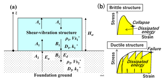
Figure 18.
Shear–vibration structure resting on foundation ground approximated by a two-layer system (a) and its stress–strain relationships and dissipated energies for brittle and ductile structures (b).
The horizontal displacement in each layer is expressed in Equations (14) and (15) using the amplitudes of upward and downward waves A1, B1 in the superstructure, and A2, B2 in the foundation ground, respectively.
The displacement u1 in the superstructure can be expressed using Equation (16) as:
where As is the amplitude at the top of superstructure. Then, the shear strain γ in the structure is given by differentiating the displacement u1 in Equation (30).
The amplitude As can be expressed by the corresponding wave energy flux dEu/dt based on the definition in Equation (7) as:
The shear strain of the superstructure in Equation (31) can be correlated with the energy flux at the ground surface by using Equations (16) and (17) as:
With the given energy flux , the induced strain γ depends on the impedance ratio α* between structure and ground, the shear stiffness of superstructure represented by Vs1*, and the first absolute value on the right side representing a resonance effect of the structure. The resonance can be dominantly large through in the resonant frequency, particularly in superstructures with smaller damping ratios D1. In such structures of small damping, therefore, not only the energy demand but also the predominant frequency of input motions other than the energy demand will be the key in the energy-based consideration. The induced strain thus evaluated from the energy flux can be compared with yield or failure strain and is correlated with different levels of structural behavior in the performance-based design.
Under strong earthquake motions, the structure exceeds a yield strain and dissipates plastic strain energy. For brittle structures with small ductility, such as slender steel structures that are easy to buckle, or masonry, brick or concrete structures without reinforcements, the maximum shear strain in a single or a small number of loading cycles may be decisive for the collapse of the structures as schematically illustrated at the top of Figure 18b. Consequently, the supplied energy flux becomes decisive for the ultimate strain as well as the resonance in predominant frequency in low-damping structures.
In contrast, for structures with higher ductility factors and higher damping such as embankments, dams, soil retaining structures and slopes, the cumulative strain by repeated loading is essential for structural performance wherein cyclically dissipated energy is compared with the supplied cumulative energy Eu as schematically illustrated in the bottom of Figure 18b. Thus, the cumulative upward wave energy Eu can be a decisive parameter in uniquely evaluating the performance of those ductile structures of higher damping.
5.2. Upward Wave Energy in View of Structural and Geotechnical Damage
As already implied in Figure 13 and Figure 14, seismic wave energy at ground surface tends to be smaller in soft-soil sites than in stiff-soil sites because, unlike the wave amplitude, it always decreases energy due to reflections passing through layer boundaries and because surface soft soils cannot store much energy due to high energy dissipation by soil damping, even in resonant frequencies. This finding may not be compatible with a widely accepted perception formed during many strong earthquakes in the past that soft-soil sites tend to undergo heavier damage than stiff-soil sites, presumably because of greater seismic energy.
During the 1923 Kanto earthquake (MW = 7.9~8.2, MJ = 7.9) in Japan, a great number of wooden houses collapsed in downtown soft-soil areas versus Pleistocene stiff-soil areas in Tokyo, triggering devastating fires and killing about 140,000 people. The similar trend seems to have occurred in the 1987 Loma Prieta earthquake (MW = 6.9), when major damage of wooden houses and lifelines was concentrated in soft-soil areas along the San Francisco Bay. However, during the 1995 Kobe earthquake (MW = 6.9, MJ = 7.2) in Japan, buildings and civil engineering superstructures were heavily damaged, killing about 5000 people in the areas composed of competent soils. In contrast, structural damage directly due to seismic inertia effect was not serious in soft-soil reclaimed areas along the seashore where geotechnical damage was prevalent due to liquefaction, only a kilometer apart from the heavily damaged areas (e.g., Matsui and Oda., 1996 [43], Tokimatsu and Asada 1996 [44]).
In discussing earthquake damage in general, one must be careful if it is structural damage directly from shaking such as failures of supporting members by inertia force or by geotechnical damage of foundations or bearing soils, which may also deteriorate superstructures indirectly.
With regard to the structural shaking damage, earthquake-induced strain in superstructures depends on, as indicated in Equation (33), the wave energy flux at the ground surface, the degree of resonance, the impedance ratio between structure and ground, and the structural rigidity. In this regard, the wave energy or energy flux at the ground surface tends to be lower in softer soils as already mentioned, which seems to be inconsistent with a generally accepted perception that the earthquake damage becomes greater in soft-soil sites.
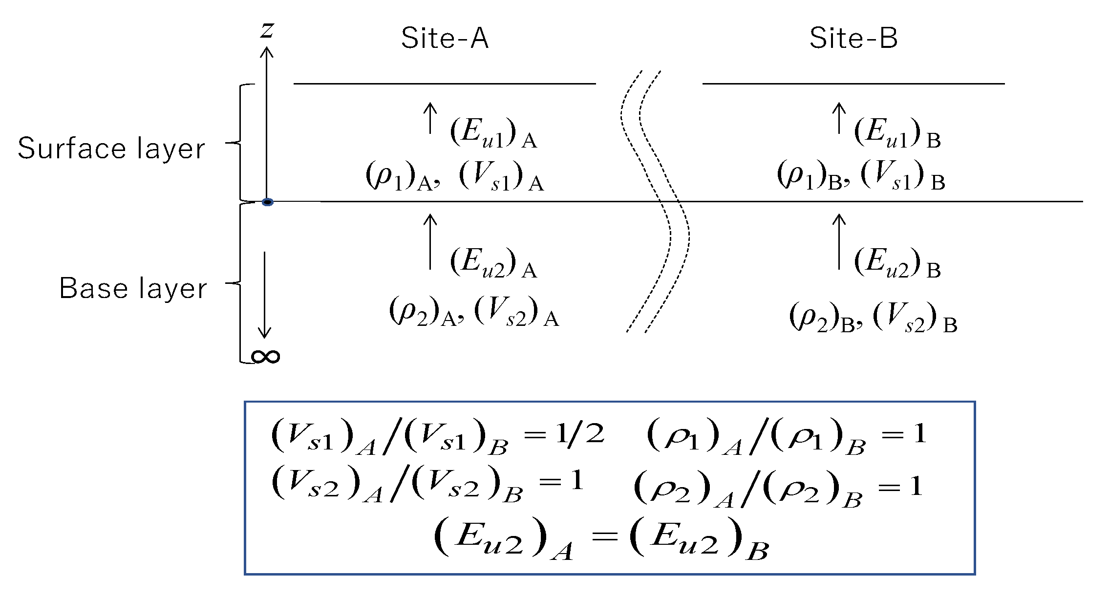
With regard to the geotechnical damage, let us compare two different site conditions A and B by using the two-layer model shown in Figure 19 (the impedance and , and the upward energy Eu1 and Eu2, in the surface and base layer, respectively). The two sites are of almost the same condition, except that Vs of the surface layer in Site A is half that in Site B. As shown in Equation (2), shear strain in the surface layer is given as γ = − /VS1 using = particle velocity of travelling wave, and hence the upward wave energy in the surface layer can be written using Equation (6) as:
or it is modified as:
The term on the left in Equation (35), cumulative squared strain in terms of time, seems to represent geotechnical damage because, for soils behaving as ductile materials, the failure is determined not by a single strain amplitude but by some sort of cumulative strain parameter, such as in Equation (35).
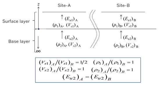
Figure 19.
Comparison of upward energy in two site conditions A and B by using a two-layer model.
Sites A and B are compared in Figure 19, assuming that (Vs1)A/(Vs1)B = 1/2 and (Vs2)A/(Vs2)B = 1, = 1, and the upward energy in the base layer is identical, (Eu)A/(Eu)B = 1. Then, the ratio of impedance ratios between Site A and Site B is expressed as αA/αB = 1/2. Using Equation (26), which is empirically derived from a number of vertical array records, the following can be obtained.
Thus, the upward energy in the surface layer in Site A becomes smaller, at 62% of Site B, whereas the cumulative strain parameter defined in Equation (35) is five times larger in Site A than Site B.
This simple example indicates that, although the upward energy at the ground surface Eu is smaller in soft soil sites than in stiff soil sites, the cumulative soil strain parameter can be larger no matter how large the Vs-difference between A and B is. This seems to be compatible with the generally accepted perception that softer soil sites tend to suffer heavier earthquake damage at least for geotechnical damage or structural damage caused by geotechnical reasons.
On structural damage directly due to seismic shaking, the effect of resonance in low-damping structures has to be properly accounted for in order to discuss if soft-soil sites are more prone to earthquake damage than stiff-soil sites. There have been quite a few reports published relatively recently, either denying a general trend of increasing structural damage in soft-soil sites or identifying decreasing structural damage by seismic inertial force with increasing geotechnical damage in soft-soil sites (Suetomi and Yoshida 1998 [45], Trifunac and Todorovska 2004 [46], Bakir et al., 2005 [47]). More investigations are certainly needed to understand this fundamental earthquake engineering topic properly, wherein the first step is to carefully classify case histories of earthquake-induced damage if they are caused directly by inertial effects on structures or indirectly by geotechnical effects.
6. Summary
In contrast to such variables as acceleration, velocity or their associated parameters, the wave energy has been limited in recognition as a demand and practical use in earthquake engineering. In this article, the energy demand in surface layers has been discussed by reviewing previous research results on SH wave energy flows in simplified two-layer systems as well as multi-layer systems in a number of vertical array recording stations during nine strong earthquakes. The following may be summarized as the significance and practicality of the energy demand concept in earthquake engineering.
- (1)
- The seismic wave energy or the energy demand is dependent not only on the particle velocity amplitude, but also on the soil impedance where the ground motion is recorded. It is meaningless to define design motions only in terms of acceleration or velocity without specifying the associated impedance value. Hence, in view of the wave energy, when a design motion is discussed, it is essential to identify the soil condition where the motion is defined.
- (2)
- The energy flow in upward and downward waves and the energy dissipation as their difference can be calculated assuming one-dimensional SH wave propagation in a horizontally layered ground. The upward wave energy as well as energy flux always tends to decrease at layer boundaries of different soil properties depending on the wave impedance ratio because a part of the energy is diverted to the wave reflected there.
- (3)
- SH wave propagation through a boundary in a two-layer model with no upper boundary in the top layer can theoretically determine the upper limit of energy supply to an overlying perfect energy absorber or ultimate earthquake energy absorbed in complete destruction of a superstructure.
- (4)
- Basic studies in simplified two-layer systems indicate that it is not easy for a soft surface layer to temporarily store large wave energy even in resonance because of large energy dissipation occurring in the soft soil during strong shaking.
- (5)
- The energy flow calculation by a number of vertical array strong motion records indicates that the upward energy tends to decrease considerably toward the ground surface in most sites mainly due to wave reflections at intermediate layer boundaries, where a large part of the energy is carried back to the earth again. The energy ratio between two arbitrary layers is approximately in proportion to the power of 0.7 of the corresponding impedance ratio.
- (6)
- Another cause of the upward energy reduction with decreasing depth is attributed to energy dissipation in near surface soft layers. High material damping values exhibited in soft soils during strong earthquakes tend to dissipate wave energy and make it difficult for the soft layers to vibrate with large energy, even in resonance.
- (7)
- In the above observation, the upward energy at the ground surface tends to be smaller in softer soils than stiffer soils. This finding seems to be incompatible with a perception widely accepted that soft-soil sites tend to suffer heavier earthquake damage than stiff-soil sites. However, the smaller upward energy in softer soils still tends to induce larger soil strains and can reasonably account for greater geotechnical damage among various earthquake damage. In this context, in statistically assessing earthquake damage, it is essential to differentiate them into direct inertial effects on structures and geotechnical effects on foundations.
- (8)
- Upward energies at the deepest levels calculated from vertical array records or those further extrapolated to seismological bedrock show a certain degree of compatibility with the well-known empirical formula, despite considerable data scatters and some gaps due to different definitions of earthquake magnitudes. Hence, the simple energy formula may be used to determine the energy demand for the energy-based design, preferably with future modifications considering fault rupture and path mechanisms specific to individual earthquakes.
- (9)
- In a performance-based design using energy, the energy demand of an earthquake may be compared directly with the energy capacity corresponding to induced strain in critical structure members. In a structure with low material damping, the degree of resonance or predominant frequency of the earthquake is another key parameter in addition to the energy flux to determine the induced strain. If the structure is ductile and of high damping, such as massive soil or concrete structures, the cumulative energy may be almost decisive in uniquely determining the performance.
- (10)
- There have been several design methodologies already developed, particularly in geotechnical engineering, wherein cumulative wave energy determines liquefaction-induced strain/settlement or slope displacement during earthquakes almost uniquely without resorting to acceleration time–histories.
Funding
This research received no external funding.
Institutional Review Board Statement
Not applicable.
Informed Consent Statement
Not applicable.
Data Availability Statement
All KiK-net data presented in this study are available for free for research purposes by accessing the website (https://www.kyoshin.bosai.go.jp/kyoshin/, accessed on 9 January 2022) of NIED, Tsukuba, Japan. Other data will be available upon request to the present author.
Acknowledgments
NIED (National Research Institute for Earth Science and Disaster Prevention) in Tsukuba, Kobe Municipal Office, KEPCO (Kansai Electric Power Company), and TEPCO (Tokyo Electric Power Company), who generously disseminated numerous vertical array data utilized in this article, are gratefully acknowledged. The great efforts in data reduction of voluminous vertical array records by former graduate and undergraduate students of Civil and Environmental Engineering Department in Chuo University are also much appreciated.
Conflicts of Interest
The author declares no conflict of interest.
References
- Sano, T. Earthquake resistant structures of building, Report of Earthquake Disaster Mitigation Committee No.83-Ko2. 1917. Available online: https://dl.ndl.go.jp/info:ndljp/pid/974342?tocOpened=1 (accessed on 9 January 2022). (In Japanese).
- Housner, G.W. Spectrum Intensities of Strong-Motion Earthquakes. In Symposium on Earthquake and Blast Effects on Structures: Los Angeles, California, June 1952; Earthquake Engineering Research Institute: Los Angeles, CA, USA, 1952; pp. 20–36. Available online: https://resolver.caltech.edu/CaltechAUTHORS:20161010-155126031 (accessed on 9 January 2022).
- NIED: National Research Institute for Earth Science and Disaster Resilience. Available online: https://www.bosai.go.jp/ (accessed on 20 December 2021).
- Gutenberg, B.; Richter, C.F. Earthquake magnitude, intensity, energy and acceleration. Bull. Seismol. Soc. Am. 1942, 32, 163–191. [Google Scholar] [CrossRef]
- Gutenberg, B.; Richter, C.F. Earthquake magnitude, intensity, energy and acceleration (Second paper). Bull. Seismol. Soc. Am. 1956, 46, 105–145. [Google Scholar] [CrossRef]
- Gutenberg, B. The energy of earthquakes. Q. J. Geol. Soc. Lond. 1956, CXII, 1–14. [Google Scholar] [CrossRef]
- Sarma, S.K. Energy Flux of Strong Earthquakes, Techtonophysics; Elsevier Publishing Company: Amsterdam, The Netherlands, 1971; pp. 159–173. [Google Scholar]
- Davis, R.O.; Berrill, J.B. Energy dissipation and seismic liquefaction of sands. In Earthquake Engineering and Structural Dynamics; Elsevier: Amsterdam, The Netherlands, 1982; No. 10; pp. 59–68. [Google Scholar]
- Kokusho, T.; Motoyama, R. Energy dissipation in surface layer due to vertically propagating SH wave. J. Geotech. Geoenviron. Eng. ASCE 2002, 128, 309–318. [Google Scholar] [CrossRef]
- Kokusho, T.; Motoyama, R.; Motoyama, H. Wave energy in surface layers for energy-based damage evaluation. Soil Dyn. Earthq. Eng. 2007, 27, 354–366. [Google Scholar] [CrossRef]
- Kokusho, T.; Suzuki, T. Energy flow in shallow depth based on vertical array records during recent strong earthquakes. Soil Dyn. Earthq. Eng. 2011, 31, 1540–1550. [Google Scholar] [CrossRef]
- Kokusho, T.; Suzuki, T. Energy flow in shallow depth based on vertical array records during recent strong earthquakes (Supplement). Soil Dyn. Earthq. Eng. 2012, 42, 138–142. [Google Scholar] [CrossRef]
- Kokusho, T. Innovative Earthquake Soil Dynamics; CRC Press, Taylor and Francis Group: Leiden, The Netherlands, 2017; Chapter 1, Section 1.2; pp. 4–10. [Google Scholar]
- Timoshenko, S.; Goodier, J.N. Theory of Elasticity; McGraw-Hill: New York, NY, USA, 1951; Chapter 14, Section 167; pp. 487–492. [Google Scholar]
- Bath, M. Earthquake energy and magnitude. Phys. Chem. Earth 1956, 23, 115–165. [Google Scholar]
- Kokusho, T.; Matsumoto, M. Nonlinearity in Site Amplification and Soil Properties during the 1995 Hyogoken-Nambu Earthquake; Special Issue of Soils and Foundations; Japanese Geotechnical Society: Tokyo, Japan, 1998; pp. 1–9. [Google Scholar]
- Schnabel, P.B.; Lysmer, J.; Seed, H.B. SHAKE—A Computer Program for Earthquake Response Analysis of Horizontally Layered Sites; Report EERC 72–12; University of California, Berkeley: Berkeley, CA, USA, 1972. [Google Scholar]
- Ishihara, K. Soil Behaviour in Earthquake Geotechnics; Oxford Science Publications: New York, NY, USA, 1996; Chapter 3, Section 3.1.3; pp. 22–28. [Google Scholar]
- Inagaki, H.; Iai, S.; Sugano, T.; Yamazaki, H.; Inatomi, T. Performance of caisson type quay walls at Kobe Port. Soils Found. 1996, 36, 119–136. [Google Scholar] [CrossRef] [Green Version]
- Kokusho, T.; Tanimoto, S. Energy capacity versus liquefaction strength investigated by cyclic triaxial tests on intact soils. J. Geotech. Geoenviron. Eng. ASCE 2021, 147, 1–13. [Google Scholar] [CrossRef]
- Joyner, W.B.; Fumal, T.E. Use of measured shear-wave velocity for predicting geologic site effects on strong ground motion. In Proceedings of the 8th World Conference on Earthquake Engineering, San Francisco, CA, USA, 21–28 July 1984; Volume 2, pp. 777–783. [Google Scholar]
- Somerville, P. Forward rupture directivity in the Kobe and Northridge earthquakes and implications for structural engineering. In Proceedings of the International Workshop on Site Response subjected to Strong Earthquake Motions, Yokosuka, Japan, 16–17 January 1996; Volume 2, pp. 324–342. [Google Scholar]
- Utsu, T. Relationships between Earthquake Magnitude Scales, Bull; ERI Earthquake Research Institute the University of Tokyo: Tokyo, Japan, 1982; Volume 57, pp. 465–497. [Google Scholar]
- Towhata, I.; Ishihara, K. Shear work and pore water pressure in undrained shear. Soils Found. 1985, 25, 73–84. [Google Scholar] [CrossRef] [Green Version]
- Yanagisawa, E.; Sugano, T. Undrained shear behaviors of sand in view of shear work. In Proceedings of the International Conference on SMFE (Special Volume on Performance of Ground and Soil Structures during Earthquakes); Balkema Publishers: New Delhi, India, 1994; pp. 155–158. [Google Scholar]
- Figueroa, J.L.; Saada, A.S.; Liang, L.; Dahisaria, N.M. Evaluation of soil liquefaction by energy principles. J. Geotech. Eng. ASCE 1994, 120, 1554–1569. [Google Scholar] [CrossRef]
- Kokusho, T. Liquefaction potential evaluation –energy-based method versus stress-based method-. Can. Geotech. J. 2013, 50, 1–12. [Google Scholar] [CrossRef]
- Kokusho, T.; Kaneko, Y. Energy evaluation for liquefaction-induced strain of loose sands by harmonic and irregular loading tests. Soil Dyn. Earthq. Eng. 2018, 114, 362–377. [Google Scholar] [CrossRef]
- Green, R.A.; Mitchell, J.K.; Polito, C.P. An energy-based excess pore pressure generation model for cohesionless soils. In Proceedings of John Booker Memorial Symposium; Balkema Publishers; Sydney, Australia, 2000. [Google Scholar]
- Law, K.T.; Cao, Y.L.; He, G.N. An energy approach for assessing seismic liquefaction potential. Can. Geotech. J. 1990, 27, 320–329. [Google Scholar] [CrossRef]
- Kayen, R.E.; Mitchell, J.K. Assessment of Liquefaction Potential During Earthquakes by Arias Intensity. J. Geotech. Geoenvironmental Eng. 1997, 123, 1162–1174. [Google Scholar] [CrossRef]
- Arias, A. A measure of earthquake intensity. In Seismic Design of Nuclear Power Plants; Hansen, R.J., Ed.; MIT Press: Cambridge, MA, USA, 1970; pp. 438–483. [Google Scholar]
- Kokusho, T.; Mimori, Y. Liquefaction potential evaluations by energy-based method and stress-based method for various ground motions. Soil Dyn. Earthq. Eng. 2015, 75, 130–146. [Google Scholar] [CrossRef]
- Kokusho, T. Liquefaction potential evaluations by energy-based method and stress-based method for various ground motions: Supplement. Soil Dyn. Earthq. Eng. 2017, 95, 40–47. [Google Scholar] [CrossRef]
- Kokusho, T. Seismic base-isolation mechanism in liquefied sand in terms of energy. Soil Dyn. Earthq. Eng. 2014, 63, 92–97. [Google Scholar] [CrossRef]
- Kokusho, T. Energy-based liquefaction evaluation for induced strain and surface settlement—Evaluation steps and case studies. Soil Dyn. Earthq. Eng. 2020, 143, 106552. [Google Scholar] [CrossRef]
- Kokusho, T.; Ishizawa, T. Energy approach to earthquake-induced slope failures and its implications. J. Geotech. Geoenviron. Eng. ASCE 2007, 133, 828–840. [Google Scholar] [CrossRef]
- Kokusho, T.; Ishizawa, T.; Koizumi, K. Energy approach to seismically induced slope failure and its application to case histories. Eng. Geol. 2007, 122, 115–128. [Google Scholar] [CrossRef]
- Kokusho, T.; Koyanagi, T.; Yamada, T. Energy approach to seismically induced slope failure and its application to case histories –Supplement. Eng. Geol. 2014, 181, 290–296. [Google Scholar] [CrossRef]
- Newmark, N.M. Effects of earthquakes on dams and embankments, Fifth Rankine Lecture. Geotechnique 1965, 15, 139–159. [Google Scholar] [CrossRef] [Green Version]
- Kokusho, T. Energy-based Newmark method for earthquake-induced slope displacements. Soil Dyn. Earthq. Eng. 2019, 121, 121–134. [Google Scholar] [CrossRef]
- Akiyama, H. Earthquake-Resistant Design Method for Buildings Based on Energy Balance; Giho-do Publishing Co.: Tokyo, Japan, 1999. (In Japanese) [Google Scholar]
- Matsui, T.; Oda, K. Foundation damage of structures, Special Issue on Geotechnical Aspects of the January 17 1995 Hyogo-ken Nambu Earthquake. Soils Found. 1996, 36, 189–200. [Google Scholar] [CrossRef] [Green Version]
- Tokimatsu, K.; Asada, Y. Effects of liquefaction-induced ground displacements on pile performance in the 1995 Hyogoken-Nambu earthquake. Soils Found. 1998, 38, 163–177. [Google Scholar] [CrossRef] [Green Version]
- Suetomi, I.; Yoshida, N. Nonlinear behavior of surface deposit during the 1995 Hyogoken-Nambu earthquake. Soils Found. 1998, 38, 11–22. [Google Scholar] [CrossRef] [Green Version]
- Trifunac, M.D.; Todorovska, M.I. 1971 San Fernando and 1994 Northridge, California, earthquakes: Did the zones with severely damaged buildings reoccur? Soil Dyn. Earthq. Eng. 2004, 24, 225–239. [Google Scholar] [CrossRef]
- Bakir, B.S.; Yilmaz, M.T.; Yakut, A.; Gulkan, P. Re-examination of damage distribution in Adapazari: Geotechnical considerations. Eng. Struct. 2005, 27, 1002–1013. [Google Scholar] [CrossRef]


Publisher’s Note: MDPI stays neutral with regard to jurisdictional claims in published maps and institutional affiliations. |
© 2022 by the author. Licensee MDPI, Basel, Switzerland. This article is an open access article distributed under the terms and conditions of the Creative Commons Attribution (CC BY) license (https://creativecommons.org/licenses/by/4.0/).