Effect of Freezing-Thawing Cycles on the Elastic Waves’ Properties of Rocks

Abstract

Freezing thawing cycles are known to play an important role in fracture propagation on rock mass and thus in rock slope instabilities. In laboratories, this phenomenon can be studied through the measurement of the velocities of elastic waves. Seven types of rocks differing by their mineralogy and texture were tested (gneiss, basalt, amphibolite, dolomite, sandstone, marble limestone and calcite). Five samples of each rock were tested. All samples were submitted to freezing/thawing cycles following the European Standard describing the tests to determine the frost resistance of natural stone. Elastic waves were recorded on the samples every 14 cycles. The experimentation continued until the rock was macrofissurated. The evolution of the weight of the samples, the velocities of elastic waves, the evolution of the shapes of the waves were recorded to characterize changes over freeze-thaw cycles. In addition, signal processing on the waves allows to compute energy variations as well as the evolution of natural frequencies of the samples.

1. Introduction

Freezing thawing (FT) cycles are supposed to play a role in fracture propagation on rock mass, and thus in rock slope instabilities [1]. The 9% water-to-ice expansion partially explain cryoclasty, but the proper mechanism is still under study [2]. Cryoclasty fragments rocks into debris of variable shape depending on the initial texture of the rocks [3]. The actual context of global warning affects the mountain cryosphere and leads to an increase in rock slopes instabilities [4,5,6]. Areas that used to be frozen all year long are now submitted to FT cycles and deteriorate faster

In laboratory, damage in rocks under FT cycles was studied by many scholars as summarized very recently in [7]. Most of the studies focus on the evolution of physical and mechanical parameters such as porosity, saturation moisture content, uniaxial compressive strength, Brazilian tensile strength and P-wave velocities (Vp). Ref. [8] for instance focused on 2 sandstones, a fine and a coarse sandstone. They showed that under freeze-thaw cycling, both rocks present the same evolution. When the number of FT cycles increase, the porosity of the two sandstones increases, with a good linear fit. They also performed triaxial tests. They showed that when FT cycles increase, UCS (uniaxial compressive strength) decreases and, considering a Mohr–Coulomb criterion, the cohesive force decreases whereas the friction angle remains constant with the increase of FT cycles. Ref. [9] studied P-wave velocity changes in freezing hard low-porosity rocks but without imposing cycles. They tested 20 alpine and 2 artic rock specimens sampled from several permafrost sites and proposed a time-average model based on their laboratory experiments.

In laboratory the increase in damage under FT cycles can be studied locally when looking at a fracture propagation with digital image correlation for instance or more globally by focusing on the evolution of damage in the rock mass with the help of velocities of elastic waves. The recording of these velocities throughout the entire experience allows to follow the evolution of damage on the same sample [8,10,11,12,13,14,15] submit six different limestones to FT cycles and notice that degradation take place in only a few cycles. For their unique type of mineralogy, the sensitivity to FT is linked to the porosity, but they emphasize the insensitivity of most of the petrophysical parameters to the FT process.

Elastic waves velocity (P-waves, but also S-waves) is a nondestructive parameter that gives information on the amount of microcracks because waves propagate better in solids than in air. Furthermore, Ref. [16] showed that the presence of liquid water (or any other low compressibility fluid) in rocks porosity influences greatly P-wave velocity value. This can be explained by a higher P-wave velocity in water (about 1500 m/s) than in air (about 331 m/s according to [17]). Thus, the degree of saturation plays an important part in the variation of P- and S-waves velocity. It is generally observed that the higher the degree of saturation, the more significant the increase of P-wave velocity [14] under usual laboratory conditions (about 20 °C). P-waves velocity, in temperate glacier ice containing liquid inclusions, is about 3660 m/s and, in moderately cold ice, it is about 3870 m/s [18]. S-waves velocities are less studied in laboratory because they are more difficult to measure, not only because of the more sophisticated experimental set-up required, but also because the shape of the waves makes it more difficult to point it properly. Nevertheless, their measurement is useful because liquid stops S-waves propagation.

In this study, we decided to explore the possibilities of using all the information about elastic waves velocities along with the evolution of the weight of the samples. Thus, we recorded their shapes and applied relatively conventional signal processing methods in the seismological domain, to identify normal frequencies and to calculate spectral energies.

2. Materials and Methods

2.1. Tested Rocks

Seven types of rocks, different in mineralogy and granulometry, but all coming from the South part of France, were tested: gneiss, basalt, amphibolite, dolomitic limestone, sandstone, marble and saccharoidallimestone.

Table 1. Mechanical and physical properties of rock types (values in italics come from bibliography).

	Density Kg/m3	Porosity %	UCS MPa	E GPa
Gneiss	2.65 × 103	1.1–3.3	25–110	7–20
Sandstone	2.15 × 103	13.7	55.5 (dry)	15
Basalt	2.97 × 103
Saccharoidallimestone	2.56 × 103
Dolomitic limestone	2.74 × 103	1–4
Marble	2.70 × 103	0.3	70–90	60–70
amphibolite	2.74 × 103	1.2	100–250

synthetizes their known physical and mechanical properties.

The gneiss comes from the site les rochers de Valabres, in the South of the French Alpes. This site has been monitored to investigate the influence of climate factors on the trigger of rock instability [19,20]. Its mineralogy consists in quartz, plagioclases (and few feldspars) and micas oriented according to its foliation. Its density is 2.65 × 10³ kg/m³. Geotechnical properties are summarized in [21]. Gneiss is anisotropic. The mechanical properties of gneiss depend on the orientation of the foliation compared to the orientation of the mechanical loading. Thus, UCS vary from 25 to 110 MPa and Young’s modulus E from 7 to 20 GPa. In our study, samples were drilled without considering the orientation of their foliation.

The amphibolite samples come from the southern part of the Massif Central. This highly fractured area underwent a strong regional metamorphism followed by a contact metamorphism (high temperature). Amphibolite contains a high concentration of amphiboles, specifically green hornblende (50%) that gave its color, but also plagioclases (20%); quartz (10%) and few other minerals such as garnet, chlorite and pyrite seams. Its density is about 2.74 × 10³ kg/m³. No mechanical test was performed on this rock, but UCS varies from 100 to 250 MPa [22]. Porosity is always very low in amphibolite, [23] gives 1.2%.

The studied marble comes from a quarry located near St Beat, in the central part of the French Pyrenees and more specifically from the Pyrenean metamorphic internal zone. Three successive tectonic events gave the rock mass a complex structure constituted by subvertical layers, despite the lack of traces of foliation due to recent metamorphism. A complete description of this marble can be found in [24,25]. Its density is about 2.70 × 10³ kg/m³, and its porosity about 0.3%. UCS = 70–90 MPa E = 60–70 GPa.

The basalt we studied is a columnar basalt that comes from the South of the Massif Central, in France. Its density is about 2.97 × 10³ kg/m³. It is an alkaline basalt with a microlithic texture: pyroxenes, olivine, plagioclases and feldspathoids in decreasing order of abundance. Two samples (R761 and R762) were drilled in height, parallel to the direction of the natural columnar basalt. The 3 other samples were drilled in width, perpendicular to the direction of the natural columns.

The dolomitic limestone studied comes from a quarry near Perpignan, in the Oriental French Pyrenees. It is a carbonated sedimentary rock; its composition is nearly 50–50 between limestone and dolomite. Bioclasts and other figurative elements can also be found. Its pinkish color is most certainly due to the presence of iron oxide most likely due to alteration. It is mainly quarried as aggregate for concrete. Its porosity is low (1–4%) and its density is about 2.74 × 10³ kg/m³.

The saccharoidallimestone comes from a quarry near Beziers, in the South of France. It is a granular sedimentary rock looking like a block of red sugar when broken into pieces. Calcite is the major mineral; it has a yellowish tint due to impurities or ion substitutions. Rare bioclasts can also be found. Its density is 2.56 × 10³ kg/m³. The block where samples were drilled was very weathered and no mechanical properties were measured. Because of its poor resistance, only few specimens were obtained (many broke during drilling) and the remaining samples are smaller than the others.

The sandstone under study is a red-brown, medium grained triangular-aged sandstone came coming from a quarry located in the East of France. It is a detritic rock, derived from the diagenesis of sand grains. Cementation was achieved by crystallizing the salts contained in seawater. Color generally depends on the content of different metals. The mineralogy of this sandstone was determined very precisely: quartz 80% and alkaline feldspars and some iron oxides 20%. Its density is about 2.15 × 10³ kg/m³, its porosity is about 13.7% UCS under dry conditions is about 55.5 MPa and UCS under saturated conditions is about 47.2 MPa; Young’s module is around 15 GPa.

Five cylindrical samples of each type of rock (50 mm in diameter, 54 to 121 mm in height) were tested except for marble where only four samples were prepared. This made it possible to derive information on properties variability. In [15], samples were cubic (5 cm squares) but [26] asks for cylindrical samples with a slenderness between 1 and 2. The use of cylindrical samples (with a slenderness between 1 and 2) is recommended by the standard to obtain cleaner signals since cylindrical samples help to avoid as much as possible waves reflection. In cubic square samples, there are more angles, and thus, more reflections are possible. It is not a great deal for P-waves, because they are fast, but it could be very difficult to find the real velocity time of S-waves in cubic samples because of too much reflection of P-waves.

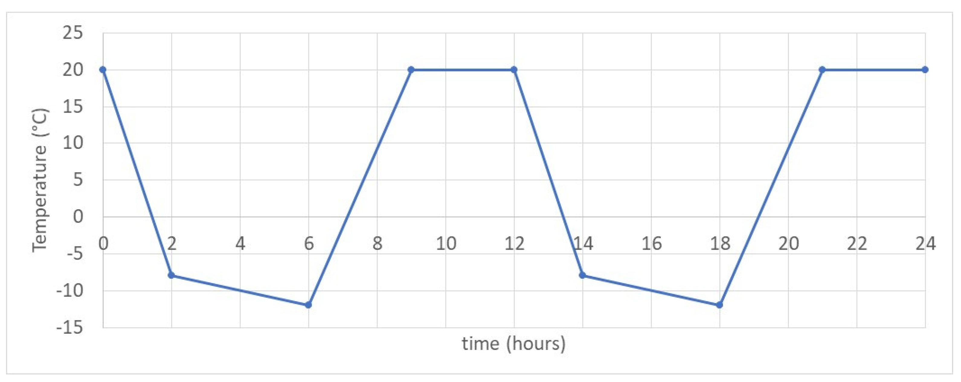
2.2. Experimental Device

The 34 samples were submitted to freeze/thaw cycles following the European Standard NF EN 12,371 [27] which measures the frost resistance of natural stone by a test comprising 2 cycles a day FT cycles, as described in Figure 1.

FT cycles were carried out in a climatic chamber. A cycle consists in a 6 h freezing period in air, followed by a 3 h thawing period during which the specimens are immersed in water, and then 3 more hours to stabilize the temperature in the sample. The freezing from 20 °C to −10 °C is obtained at 2 freezing rates: from 20 °C to −8 °C in 2 h and then from −8 °C to −12 °C in 4 h. Thawing is performed under a constant rate, from −12 °C to 20 °C in 3 h. Once a week, i.e., every 14 cycles, samples are taken out the climatic chamber to perform measurements. The cycles are repeated until the specimens broke, or up to the given maximum number of cycles (70 cycles).

Elastic waves velocities (Vp, Vs1 and Vs2) were measured according to the French standard NF P 94-411 [26]. The accuracy of those measurements depends essentially on the selected electrical pulse generator. The system is presented in Figure 2.

It consists in:

• An electric pulse generator that can generate P-wave, and two S-waves, S1 and S2, perpendicular to one another;
• A transmitter and a receiver for P- and S-waves;
• A transducer used to control the force applied by the pump on the test; the contact is systematically obtained under a 2 kN load to be strictly reproductible and to be able to compare results.

In addition of quantifying the velocity of elastic waves once a week, the samples taken out the climatic chamber were also measured in length and weight. The measurements were performed after the temperature in the climatic chamber reached 20° for nearly 2 h.

2.3. Signal Processing

There are two ways to visualize a signal: temporal representation and frequency representation. The temporal representation is the one registered when studying velocities of elastic waves. However, it can be interesting to observe the frequency content of a signal to better visualize its characteristics. Signal processing consists in performing mathematical processing in order to obtain the frequency response of the processed signal. This response makes it possible to determine the characteristic frequencies, but also the energy involved, as well as to verify the quality of the signal. To transform a function in a time domain f(t) to a function in a frequency domain F(s), the Fourier transform is probably the most used Equation (1), with i, complex number defined by i² = 1:

$$F\left(s\right)=\underset{+\infty }{\overset{-\infty }{{\displaystyle \int }}}f\left(t\right)e^{-ist}dt$$

(1)

The Fourier transform is only applicable to continuous functions. However, the signal recorded in the laboratory is a sampled signal, s(n), where n can take N values. In this case, the discrete Fourier transform Equation (2) is used:

$$S\left(k\right)={\displaystyle \sum }_{n=0}^{N-1}s\left(n\right) e^{-2i\pi k\frac{n}{N}}$$

(2)

As any recorded signal has a clear beginning and an end, a rectangular window was applied to the signal [28]. Although, applying a rectangular window result, in frequency, in a convolution between the spectrum of the analyzed signal and the window and produces secondary lobes and intensifies the main lobe. To overcome this, it is possible to apply a chosen window. [29] considers that the Hamming window Equation (3) is the best compromise between the resolution obtained in frequency and the resolution obtained in amplitude.

$$0.54 \pm 0.46 \cos \left(\frac{2\pi }{N}n\right)$$

(3)

Finally, we also calculated the spectral energies (En) following Equation (4).

$$En={\displaystyle \sum }_{n=-\infty }^{+\infty }{\left|S\left(k\right)\right|}^2$$

(4)

3. Results

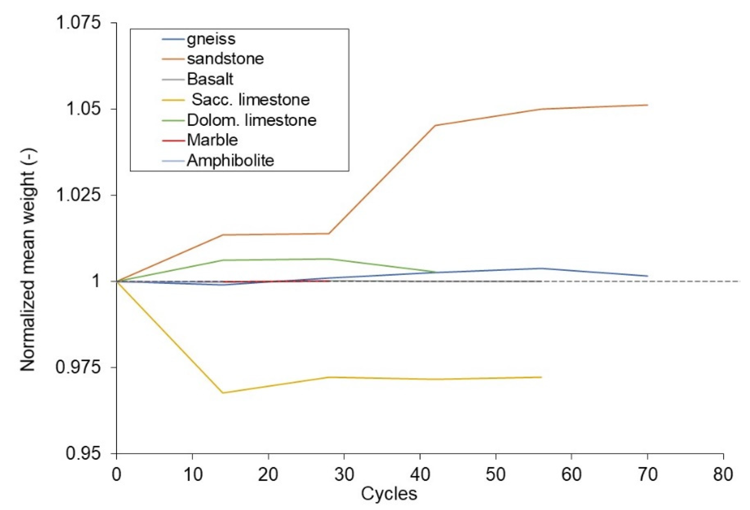
3.1. Macroscopic Observations and Evolution of the Weight of the Samples

Figure 3 displays samples photos at the end of the experiments, and

Table A1. Evolution of the weight of the samples.

	Samples Weight (g)
Cycle	Samples	Gneiss	Sandstone	Basalt	Saccharoidal Limestone.	Dolomitic Limestone.	Marble	Amphibolite
0	1	464.37	379.37	509.68	278.85	659.85	1520.01	538.12
	2	450.51	375.31	509.89	265.98	654.71	1538.91	517.79
	3	493.71	372.07	498.21	276.17	675.24	1527.66	638.60
	4	497.91	372.08	491.84	283.93	984.14	1529.34	616.44
	5	498.33	377.19	496.07	253.65	992.97		626.98
	mean	480.97	375.20	501.14	271.72	793.38	1528.98	587.59
14	1	463.92	383.41	509.70	270.44	663.00	1520.01	538.13
	2	450.09	380.66	509.93	261.25	660.68	1538.91	517.82
	3	493.10	375.81	498.20	274.36	677.14	1527.66	638.61
	4	497.46	377.82	491.81	263.14	990.84	1529.34	616.48
	5	497.73	383.72	495.73		999.76		627.01
	mean	480.46	380.28	501.07	267.30	798.28	1528.98	587.61
28	1	464.86	384.46	509.81	271.67	662.65	1519.93
	2	450.99	380.65	509.99	263.14	661.39	1539.14
	3	494.30	375.95	498.52	276.11	676.57	1527.70
	4	498.47	377.87	491.98	263.34	991.52	1529.89
	5	498.79	383.18	495.95		1000.76
	mean	481.48	380.42	501.25	268.57	798.58	1529.17
42	1	465.64	396.01	509.72	271.73	662.54
	2	451.65	391.58	509.92	262.24
	3	494.87	388.48	498.28	276.24	676.30
	4	498.95	389.72	491.81	263.34
	5	499.94	395.13	495.76
	mean	482.21	392.18	501.10	268.39	669.42
56	1	465.47	398.44	509.64	271.16
	2	451.79	393.24	509.83	262.45
	3	497.81	390.28	498.72	276.61
	4	499.16	391.46	491.72	263.98
	5	499.82	396.28	495.63
	mean	482.81	393.94	501.11	268.55
70	1	464.68	399.23
	2	450.72	393.67
	3	494.72	390.69
	4	499.07	391.51
	5	499.59	396.88
	mean	481.76	394.40

provided in Appendix A presents the variation of the weight of all samples during experiment. The lack of a weight value in Table 1 indicates that the sample is broken and cannot be measured further.

From a macroscopic point of view, rocks react differently to FT cycles. Amphibolite samples are the most sensitive since all amphibolite samples broke between 14 and 28 cycles. It is impossible to be more precise, because the frost chamber was only opened every 14 cycles. On the opposite, all of gneiss and sandstone samples remained unbroken even after 70 cycles. Between those two extremes, one of the saccharoidal limestone sample broke before reaching 28 FT cycles whereas the other four resisted more than 56 FT cycles. Looking more closely at the pictures (Figure 3) we can observe two different types of failure. Large failure is observed in saccharoidal limestone and dolomitic limestone. Sample are cut from part to part and sometimes in pieces, whereas for the other rocks, failure occurs more superficial: only small parts of the sample are lost just like peeling.

On Figure 4, we chose to represent the evolution of the normalized mean weight of the samples. The detail of the variations in weights over FT cycles for all rocks is given in Appendix A. The European standard for frost resistance requests for a weighing instrument with an accuracy of at least 0.01% of the mass to be weighed and this explains the two digits precision given in the table. Despite this accuracy, the variations in weight of the samples with the number of FT cycles do not show a precise trend for five of the seven types of rocks, that is gneiss, basalt, marble and amphibolite. However, the saccharoidal limestone samples significantly lose weight, which we explain by the deterioration of the samples with a loss of grains or of very small pieces. Conversely sandstone samples gain weight. We attribute this gain to the increase of water content because sandstone is the only rock under study that has a sufficient porosity to enable entrance of water into its pores.

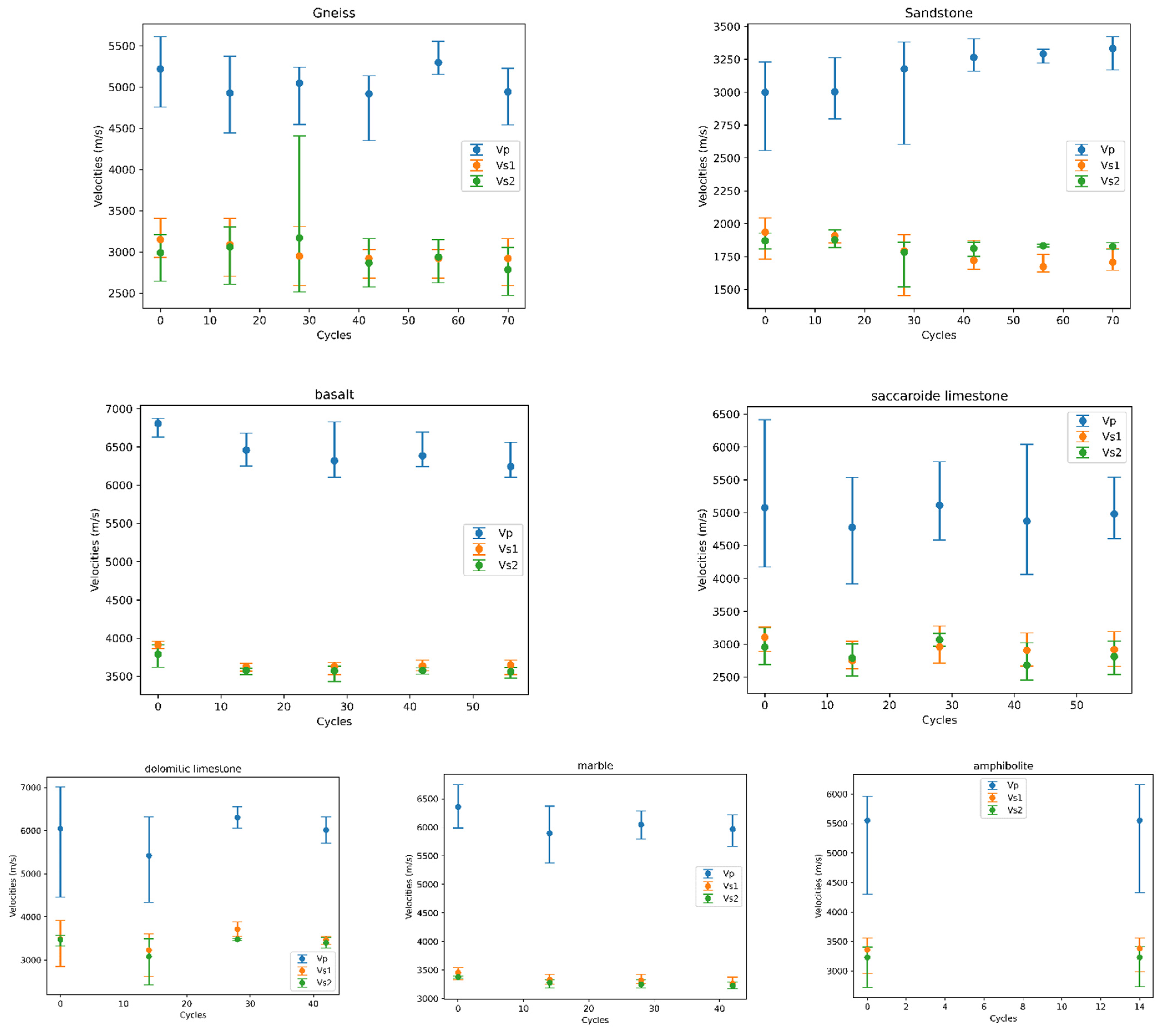
3.2. Velocities of Elastic Waves

3.2.1. General Evolution

Figure 5 and Figure 6 present the evolution of the elastic waves’ velocities measured in the samples during the experiment. Figure 5 presents the evolution of the normalized mean P-waves and S1-waves for all the rock types while Figure 6 presents the evolution, of the mean value together with the min and max registered to illustrate the spread of results. Values are normalized by the initial mean.

A decrease of velocities of waves was expected linked to damage progression. Yet, only basalt and marble present a P-waves decrease, even if the decrease is slight. A very slight decrease can also be observed on S-waves. The P-waves decrease is consistent with development of damage in the samples as can be observed macroscopically with first with the identification of microcracks, and then, secondly, with the coalescence of those cracks leading to fracturation of the samples (as can be seen on Figure 3, Figure 4 and Table 1).

Damage index [30], ref. [31] was also computed but it did not give any new indication for interpretation.

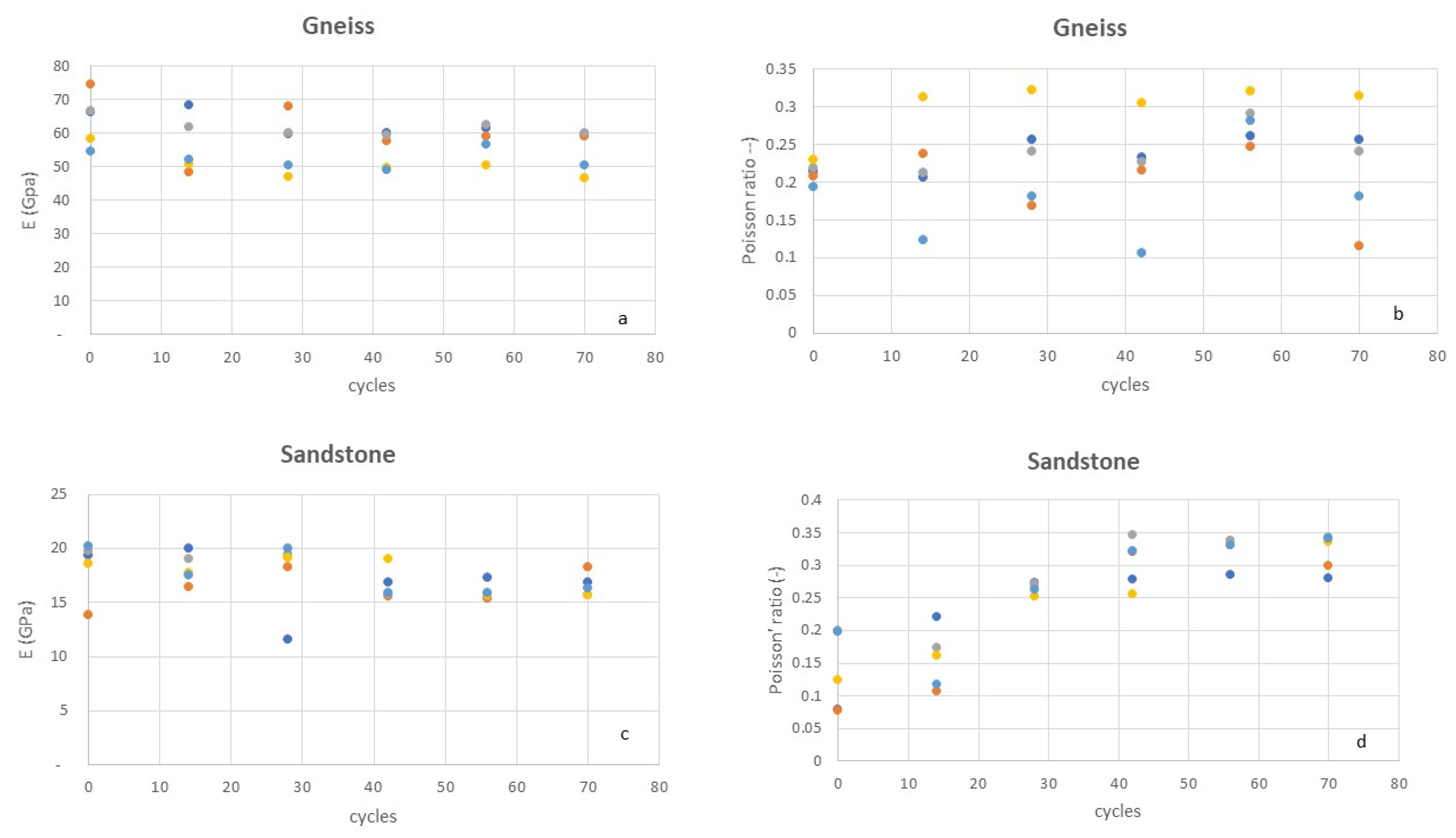
3.2.2. Dynamic Elastic Modulus and Poisson Ratio

The bulk density ρ of the samples and the velocities of the elastic waves measurements can be used to calculate the dynamic Young’s modulus (E_d) and the dynamic Poisson ratio (ν_d) [16], according to equations:

$${\mathrm{E}}_{\mathrm{d}}=\mathsf{\rho }\frac{{\mathrm{V}}_{\mathrm{s}}^2\left(3{\mathrm{V}}_{\mathrm{p}}^2-4{\mathrm{V}}_{\mathrm{s}}^2\right)}{\left({\mathrm{V}}_{\mathrm{p}}^2-{\mathrm{V}}_{\mathrm{s}}^2\right)}$$

(5)

$${\mathsf{\nu }}_{\mathrm{d}}=\frac{\left({\mathrm{V}}_{\mathrm{p}}^2-2{\mathrm{V}}_{\mathrm{s}}^2\right)}{2\left({\mathrm{V}}_{\mathrm{p}}^2-{\mathrm{V}}_{\mathrm{s}}^2\right)}$$

(6)

E_d and ν_d were calculated only with Vs2 because whereas, for two samples (R754 gneiss and R764, saccharoidal limestone) unacceptable negative values of Poisson ratio would have been obtained. We chose to represent on Figure 7 only the evolutions obtained on gneiss and sandstone as they are the most representative. Nevertheless, all results are discussed. Gneiss and marble present the same evolution: when FT cycles increase E_d modules decrease and ν_d remain constant. Basalt, dolomitic limestone and saccharoidal limestone behave in the same way: when FT cycles increase, E_d decrease very slightly and ν_d remain constant. Only sandstone presents a very different evolution: when FT cycles increase E_d decrease very slightly and ν_d increase (Figure 7).

3.2.3. Evolution of V_p/V_s Ratio

The V_p/V_s ratio was computed with Vs1 and Vs2 for each specimen. Curves are not presented, as ratios remain globally constant with the increase of the number of cycles. The value of the ratio depends on the rock tested: 1.68 for amphibolite, 1.71 for gneiss, 1.72 for saccharoidal limestone, 1.74 for dolomitic limestone, 1.76 for basalt and 1.83 for marble. The V_p/V_s ratio of the sandstone is the only one that changes clearly with the number of FT cycles going from 1.57 (initial) to 1.89 (after 70 FT cycles).

3.2.4. Evolution of Vs1/Vs2 Ratio

Vs1/Vs2 ratio was also calculated but remained nearly constant when FT cycles increased. This was observed for all samples.

3.3. Frequency Analysis

As explained in 2.2, all transmitted and received signals of each sample were recorded and then processed. It is important to note that signal processing was also performed on empty device to identify the natural frequency of the system. Thus, we were able to plot amplitude as a function of frequencies for V_p, Vs1 and Vs2, for each sample. On Figure 8, we selected only one representative evolution of V_p, Vs1 or Vs2 per types of rock, even if the 102 plots (34 samples × 3 waves) were analyzed.

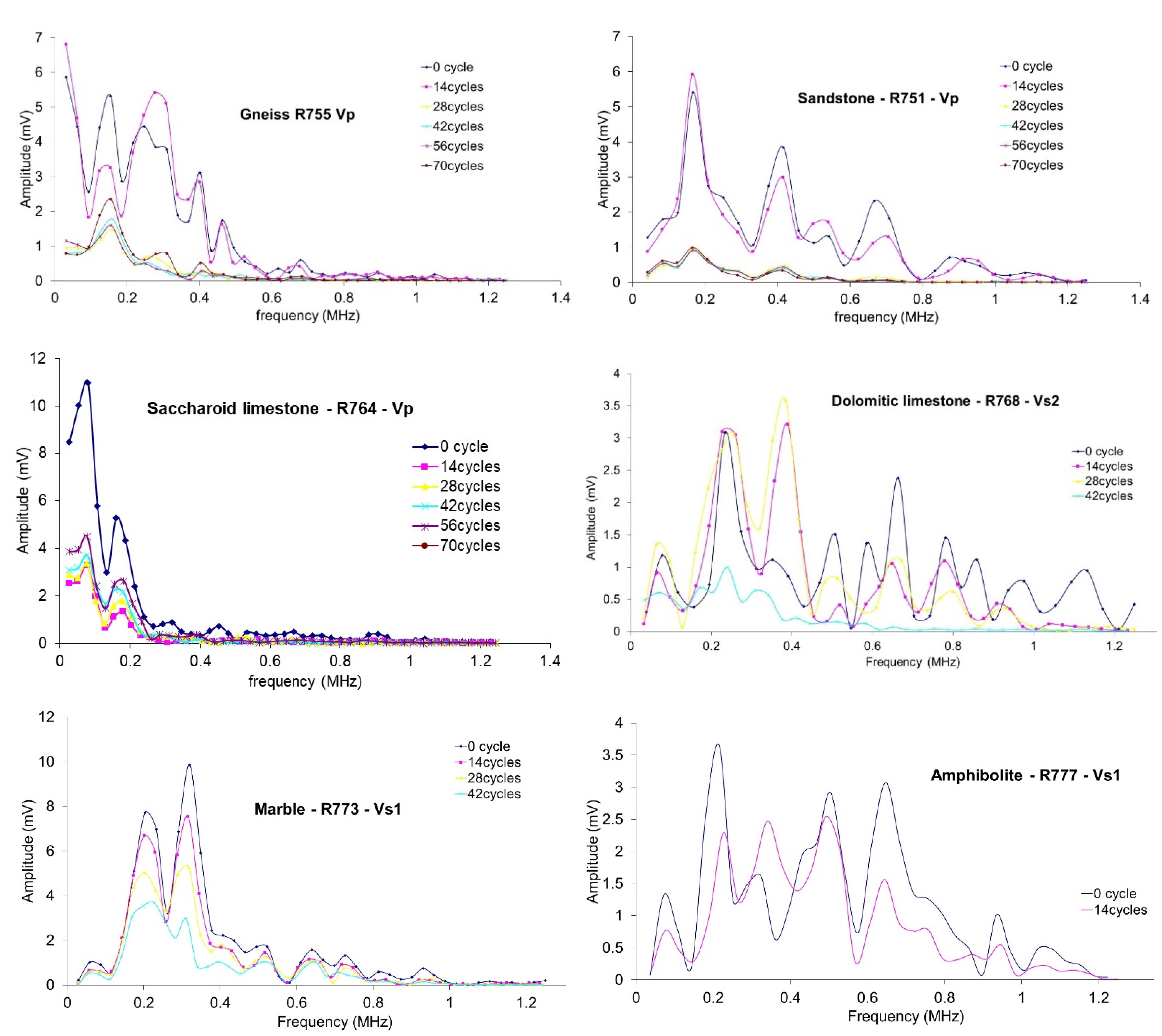
3.3.1. Observations on the Evolution of Spectrum Amplitude

The first important observation is that samples from the same mineralogy behave in the same way. However, depending on the tested mineralogy, the evolution of amplitude with the number of cycles varies. If we analyze the results more precisely, we can observe:

• Sandstone: Evolution of the frequency is the same regardless of the type of waves P, S1 and S2. Sandstone has very large and comparable amplitudes for 0 and 14 cycles, and very small (and comparable) amplitude afterwards;
• Basalt and dolomitic limestone: When FT cycles increase, a regular decrease of the V_p amplitudes is observed. “Regular” means that after each set of 14 cycles, V_p amplitude decreases. This decrease is also observed on Vs1 and Vs1 but less regular (i.e., globally, amplitude of n cycles is superior to amplitude of (n + 14) cycles, but it can be not true punctually);
• Marble: when FT cycles increase a regular decrease of the V_p, Vs1 and Vs2 amplitudes is obtained;
• Amphibolite: it seems to behave as marble but with only two curves (0 and 14 cycles) it is difficult to conclude on a trend;
• Gneiss and saccharoidal limestone: No global trend is observed on all samples. Moreover, 3/5 gneiss samples behave as sandstone but the other two do not.

3.3.2. Observations on the Evolution of Spectrum Frequencies

All frequencies peaks were recorded to identify a possible trend. We were able to show that all frequencies peaks obtained on the sample in its natural state (0 cycles) can still be observed after many FT cycles. In the meantime, no new peak seems to appear when FT cycles increase. Unfortunately, we were not able to distinguish typical frequencies corresponding to each mineralogy.

3.4. Spectral Energies

The spectral energy of the all the signals was calculated, as described in 2.3. It evolves during the FT cycles without marked trend, except that the last energy measured before rupture is always much lower than all the previous ones. On gneiss, basalt and saccharoidal limestone a slight increase of energy is observed during cycles; contrarywise on marble, a decrease is observed on three of the four studied samples.

4. Discussion and Conclusions

Seven types of saturated rocks were subjected to freeze-thaw cycles. Every 14 cycles, the weight and dimensions of the samples as well as the waveform of elastic waves velocities (P-waves and S1- and S2-waves) were recorded. All rocks, except for gneiss and sandstone, broke before 70 cycles. Some of them (amphibolite) for less than 28 cycles. Samples of a rock type are consistent with each other. However, even after carefully analyzing the results, no clear proper trend of damage was highlighted before failure occurred. It is difficult to propose any indicator explaining the different behaviors of the seven types of rocks and the behavior of each type. The sandstone is the only one that has concomitant variations: dynamic Young’s modulus and V_P increase while V_P/V_S and coefficient of Poisson decrease when FT cycles increase, which is consistent with water intake.

The elastic waves velocities that were used in our experiment, is a well-known and good indicator to observe the evolution of damage. Yet, all samples except those of gneiss and sandstone present a slight P-waves slight decrease. Nonetheless, this decrease remains small, and much slighter that expected considering the final failure and V_p decrease observed during other types of tests. For example, on limestone samples submitted to thermal cycles [10], V_p velocities can decrease by more than 10% before failure, and moreover, a decrease of about 20% was noticed by [11] before failure during a triaxial test. However, all these observations were achieved on dry samples. As shown in [32] when the degree of saturation of clayey soil blocs decreases, both P- and S-waves velocities increased whereas on non-clayey materials the opposite behavior is generally observed: V_p increases when the degree of saturation increases [33]. Thus, if for sandstone the gain of weight during the experiment is assimilated to an increase of water content, the evolution of velocities is consistent.

Signal processing made it possible to find characteristic frequencies for each of the tested mineralogies, but the observed evolution of the pic values is considered not significant so far, and we plan to reprocess the signals to propose proper conclusions.

Moreover signal-processing could give further clues to evaluate the state of the samples. It was previously observed [34] that damage that occurs in a rock submitted to a triaxial test resulted in an increase in energy, then a sharp decrease that directly preceded the phase of rupture. In our experiments we observed a global decrease in energy when comparing the initial and the last measurements, but, once again, no systematic observation could be performed. In addition, the signal waveform as well as the frequency content, the evolution of amplitude or spectral energy was studied. Despite deep analyses it seems that none of the indicators monitored made it possible to detect significant changes during the FT cycles, at least, if we want to identify one unique indicator for all the rocks.

Porosity was not precisely studied because it was not initially planned for these samples. For further investigation, it will be planned to differentiate pore from crack porosity and intergranular from diagenetic porosity for sedimentary rocks, and to look in detail at microscopic aspects of porosity

In agreement with [15], our results confirm that the number of FT cycles should be increased to 100 if samples do not break before. Because of the rapid evolution of the degradation the test could also be shifted in time for half of the samples. For example, we propose to begin the cycles of half of the samples, 7 days later. When the first samples break, time between the measurements of the second samples should be shortened. The exact value of the shortening would be studied.

References

1. Hall, K. Evidence for freeze-thaw events and their implications for rock weathering in northern Canada. Earth Surf. Process. Landf. 2004, 29, 43–57. [Google Scholar] [CrossRef]
2. Hallet, B. Why do freezing rocks break? Science 2006, 314, 1092–1093. [Google Scholar] [CrossRef]
3. Draebing, D.; Krautblatter, M. The Efficacy of Frost Weathering Processes in Alpine Rockwalls. Geophys. Res. Lett. 2019, 46, 6516–6524. [Google Scholar] [CrossRef]
4. Eppes, M.C.; Hancock, G.S.; Kiessling, S.; Moser, F. Rates of subcritical cracking and long-term rock erosion. Geology 2018, 46, 951–954. [Google Scholar] [CrossRef]
5. Ravanel, L.; Magnin, F.; Deline, P. Impacts of the 2003 and 2015 summer heatwaves on permafrost-affected rock-walls in the Mont Blanc massif. Sci. Total Environ. 2017, 609, 132–143. [Google Scholar] [CrossRef]
6. Magnin, F.; Westermann, S.; Pogliotti, P.; Ravanel, L.; Deline, P.; Malet, E. Snow control on active layer thickness in steep alpine rock walls (Aiguille du Midi, 3842 m a.s.l., Mont Blanc massif). Catena 2017, 149, 648–662. [Google Scholar] [CrossRef]
7. Deprez, M.; de Kock, T.; de Schutter, G.; Cnudde, V. A review on freeze-thaw action and weathering of rocks. Earth-Sci. Rev. 2020, 203, 103143. [Google Scholar] [CrossRef]
8. Liping, W.; Ning, L.; Jilin, Q.; Yanzhe, T.; Shuanhai, X. A study on the physical index change and triaxial compression test of intact hard rock subjected to freeze-thaw cycles. Cold Reg. Sci. Technol. 2019, 160, 39–47. [Google Scholar] [CrossRef]
9. Draebing, D.; Krautblatter, M. P-wave velocity changes in freezing hard low-porosity rocks: A laboratory-based time-average model. Cryosph. Discuss. 2012, 6, 1163–1174. [Google Scholar] [CrossRef]
10. Villarraga, C.J.; Gasc-Barbier, M.; Vaunat, J.; Darrozes, J. The effect of thermal cycles on limestone mechanical degradation. Int. J. Rock Mech. Min. Sci. 2018, 109, 115–123. [Google Scholar] [CrossRef]
11. Fortin, J.; Schubnel, A.; Guéguen, Y. Elastic wave velocities and permeability evolution during compaction of Bleurswiller sandstone. Int. J. Rock Mech. Min. Sci. 2005, 42, 873–889. [Google Scholar] [CrossRef]
12. Fortin, J.; Gasc-barbier, M.; Merrien-soukatchoff, V. Comportement des roches en température. In Thermomécanique Des Roches; Gasc-Barbier, M., Merrien-Soukatchoff, V., Berest, P., Eds.; Presses des Mines: Paris, Frence, 2018. [Google Scholar]
13. Vagnon, F.; Colombero, C.; Colombo, F.; Comina, C.; Ferrero, A.M.; Mandrone, G.; Vinciguerra, S.C. Effects of thermal treatment on physical and mechanical properties of Valdieri Marble—NW Italy. Int. J. Rock Mech. Min. Sci. 2019, 116, 75–86. [Google Scholar] [CrossRef]
14. Vagnon, F.; Colombero, C.; Comina, C.; Ferrero, A.M.; Mandrone, G.; Missagia, R.; Vinciguerra, S.C. Relating physical properties to temperature-induced damage in carbonate rocks. Geotech. Lett. 2021, 11, 1–11. [Google Scholar] [CrossRef]
15. Martínez-Martínez, J.; Benavente, D.; Gomez-Heras, M.; Marco-Castaño, L.; García-Del-Cura, M.Á. Non-linear decay of building stones during freeze-thaw weathering processes. Constr. Build. Mater. 2013, 38, 443–454. [Google Scholar] [CrossRef]
16. Gueguen, Y.; Palciauskas, V. Introduction to the Physics of Rocks; Pricetown University Press: Pricetown, UK, 1994. [Google Scholar]
17. Lama, R.D.; Vutukuri, V.S. Handbook on Mechanical Properties of Rocks, 2nd ed.; Trans Tech Publications: Clausthal, Germany, 1978. [Google Scholar]
18. Lliboutry, L. le fluage de la glace. La Houille Blanche 1970, 56, 489–492. [Google Scholar] [CrossRef] [Green Version]
19. Gunzburger, Y.; Merrien-Soukatchoff, V.; Guglielmi, Y. Influence of daily surface temperature fluctuations on rock slope stability: Case study of the Rochers de Valabres slope (France). Int. J. Rock Mech. Min. Sci. 2005, 42, 331–349. [Google Scholar] [CrossRef]
20. Merrien-Soukatchoff, V.; Clément, C.; Senfaute, G.; Gunzburger, Y. Monitoring of a potential rockfall zone: The case of ‘Rochers de Valabres’ site. In Proceedings of the International Conference on Landslide Risk Management, Vancouver, BC, Canada, 31 May–3 June 2005; pp. 416–422. [Google Scholar]
21. Clément, C.; Merrien-Soukatchoff, V.; Dünner, C.; Gunzburger, Y. Stress measurement by overcoring at shallow depths in a rock slope: The scattering of input data and results. Rock Mech. Rock Eng. 2009, 42, 585–609. [Google Scholar] [CrossRef]
22. Hoek, E. Rock Mechanics Laboratory Testing in the Context of a Consulting Engineering Organization. Int. J. Rock Mech. Min. Sci. 1977, 14, 93–101. [Google Scholar] [CrossRef]
23. Zharikov, A.V.; Pek, A.A.; Lebedev, E.B.; Dorfman, A.M.; Zebrin, S.R. The effects of water fluid at temperatures up to 850 °C and pressure of 300 MPa on porosity and permeability of amphibolite. Phys. Earth Planet. Inter. 1993, 76, 219–227. [Google Scholar] [CrossRef]
24. Gasc-Barbier, M.; Hoang, T.T.N.; Marache, A.; Sulem, J.; Riss, J. Morphological and mechanical analysis of natural marble joints submitted to shear tests. J. Rock Mech. Geotech. Eng. 2012, 4, 296–311. [Google Scholar] [CrossRef]
25. Gasc-Barbier, M.; Virely, D.; Guittard, J.; Merrien-Soukatchoff, V. Different approaches to fracturation of marble rock—The case study of the St Beat tunnel (French Pyrenees). In Proceedings of the International Society for Rock Mechanics, Liege, Belgium, 9–12 May 2006; pp. 619–623. [Google Scholar] [CrossRef]
26. Afnor—French Standard. NF P94-411—Rock—Determination of the Ultrasonic Waves Velocity in Laboratory—Transmission Method. 2002. Available online: www.afnor.fr (accessed on 21 January 2022).
27. Afnor—European Standard. NF EN 12371—Natural Stone Test Methods—Determination of Frost Resistance. 2010. Available online: www.afnor.fr (accessed on 21 January 2022).
28. Wanatabe, T.; Sassa, K. Velocity and Amplitude of P-Waves Transmitted through Fractured zones composed of Multiple Thin Low-velocity Layers. Int. J. Rock Mech. Min. Sci. Geomech. 1995, 32, 313–324. [Google Scholar] [CrossRef]
29. Harris, F.J. On the use of windows for harmonic analysis with the discrete Fourier transform. Proc. IEEE 1978, 66, 51–83. [Google Scholar] [CrossRef]
30. Denis, A.; Panet, M.; Tourenq, C. Rock identification by means of continuity index. In Proceedings of the 4th International Congress on Rock Mechanics, Montreux, Suisse, 2–8 September 1979; p. 125. [Google Scholar]
31. Klimis, N. Geothechnical characterization of a thermal cracked marble. In Proceedings of the 7th International Congress on Rock Mechanics, Aachen, Deutschland, 16–20 September 1991; pp. 353–361, ISBN 90 5410 0141. [Google Scholar]
32. Aubert, J.E.; Gasc-Barbier, M. Hardening of clayey soil blocks during freezing and thawing cycles. Appl. Clay Sci. 2012, 65–66, 1–5. [Google Scholar] [CrossRef]
33. Yu, G.; Vozoff, K.; Durney, D.W. Effects of confining pressure and water saturation on ultrasonic compressional wave velocities in coals. Int. J. Rock Mech. Min. Sci. Geomech. Abstr. 1991, 28, 515–522. [Google Scholar] [CrossRef]
34. Martınez-Martinez, J.; Benavente, D.; Ordonez, S.; Garcıa-del-Cura, M.A. Multivariate statistical techniques for evaluating the effects of brecciated rock fabric on ultrasonic wave propagation. Int. J. Rock Mech. Min. Sci. 2008, 45, 609–620. [Google Scholar] [CrossRef]
Figure 1. One day cycles of imposed temperature (2 cycles per day).
Geosciences 12 00103 g001
Figure 2. Experimental device (a) and representative waveforms of the receive signal: (b) P-wave, (c) S1-wave and d S2-wave. On (bd): in blue the electric pulse and in red, the received signal.
Geosciences 12 00103 g002
Figure 3. Samples at the end of experiments.
Geosciences 12 00103 g003
Figure 4. Evolution of the normalized mean weight of the samples. Values are normalized by the initial mean—the dot line corresponds to constant weight. Amphibolite and marble do not vary, their curves are hidden by basalt.
Geosciences 12 00103 g004
Figure 5. Evolution of the normalized mean P-waves (a) and S1-waves (b) of the samples—values are normalized by the initial mean.
Geosciences 12 00103 g005
Figure 6. Evolution of the velocities of elastic waves for the tested rocks (Vp in blue, Vs1 in orange and Vs2 in green) max, mean and min values are given to illustrate the spread of results. The rock type is mentioned above each graph.
Geosciences 12 00103 g006
Figure 7. Evolution of dynamic Modulus (a,c) and Poisson’ ratio (b,d) calculated according to Equations (1) and (2) for gneiss (a,b) and sandstone (c,d) samples.
Geosciences 12 00103 g007
Figure 8. P-wave and S-wave frequency spectrum—a set of spectra (1 sample, only Vp, Vs1 or Vs2) is given for each mineralogy). The rock type is mentioned in each graph.
Geosciences 12 00103 g008