The Potential Use of Ground Conductivity Meters to Identify the Location of Seepages—Case Study of the Maniów Levee near Krakow, Poland


Abstract
1. Introduction
2. Case Study: Geological Formation and Geotechnical Parameters
3. The Conductivity of the Soil, Rocks, and Water
4. Methods
4.1. Potential of the GCM Method in Identifying the Location of Seepages in Levee Zones
4.2. Field Measurements
5. Processing the Measurement Data
6. Locating the Seepage Zones
7. Conclusions
Author Contributions
Funding
Acknowledgments
Conflicts of Interest
References
- ADRC (Asian Disaster Reduction Center). Information on Disaster Risk Reduction of the Member Countries. Available online: http://www.adrc.asia/nationinformation.php?NationCode=50&Lang=en&Mode=country (accessed on 31 July 2018).
- INFORM (Index for Risk Management). Available online: http://www.inform-index.org/ (accessed on 25 July 2018).
- Okaka, O.O.; Odhiambo, D.O. Health vulnerability to food-induced risks of households in food-prone informal settlements in the Coastal City of Mombasa, Kenya. Nat. Hazards 2019, 99, 1007–1029. [Google Scholar] [CrossRef]
- Hayashi, K.; Abe, T.; Tanaka, T.; Konishi, C. Application of integrated geophysical method to levee evaluation. In Proceedings of the Fourth International Conference on Scour and Erosion, Tokyo, Japan, 5–7 November 2008; pp. 295–301. [Google Scholar]
- Ferriz, H. Use of geophysics for levee investigation. In Proceedings of the Levee State of Practice Symposium, Turlock, CA, USA, 22 April 2016. [Google Scholar]
- Gillip, J.A.; Payne, J.D. Geophysical Characterization of the Lollie Levee near Convay, Arkansas Using Capacitively Coupled Resistivity Survey, Coring and Direct Push Logging; U.S. Geological Data Series Report 640; U.S. Geological Survey: Reston, VA, USA, 2011; 27p. [Google Scholar]
- Cygal, A.; Stefaniuk, M.; Kret, A.; Kurowska, M. The application of electrical resistivity tomography (ERT), induced polarization (IP) and electromagnetic conductivity (EMC) methods for the evaluation of the technical condition of flood embankment corpus. Geologia 2016, 42, 279–287. [Google Scholar] [CrossRef]
- Cygal, A.; Borecka, A.; Stefaniuk, M.; Sada, M.; Ważny, J. Multivariate interpretation geophysical data for evaluation of geotechnical condition of part embankment Vistula river. In Proceedings of the CAGG AGH Conference, Kraków, Poland, 10–13 September 2019. [Google Scholar]
- Jokiel, P.; Pociask-Karteczka, J.; Marszelewski, W. Hydrologia Polski; PWN: Warszawa, Poland, 2017; pp. 160–167. (In Polish) [Google Scholar]
- Jokiel, P.; Tomalski, P. Sezonowość odpływu z wybranych zlewniach karpackich. Przegląd Geograficzny 2017, 89, 29–44. (In Polish) [Google Scholar] [CrossRef]
- Mosiej, K.; Abramczuk, W.; Mosiej, U.; Drążek, A.; Pawlicka, T. Ekspertyza Stanu Technicznego Budowli Hydrotechnicznej tj. Prawego Wału Przeciwpo-Wodziowego Rzeki Wisły na Odcinku Wału km 34+270–38+350 (co Odpo-Wiada km Rzeki 197+450–202+300). Położonego w Miejscowości Maniów, gm. Szczucin, Pow. Dąbrowski; Biuro Bad-Projekt-Wykonaw Aqua-Geo: Warszawa, Poland, 2014. (In Polish) [Google Scholar]
- Walczowski, A. Objaśnienia do Szczegółowej Mapy Geologicznej Polski. Arkusz Pacanów (M34-55C); Wydawnictwa Geologiczne: Warszawa, Poland, 1968. (In Polish) [Google Scholar]
- Plewa, M.; Plewa, S. Petrofizyka; Wydawnictwa Geologiczne: Warszawa, Poland, 1992. (In Polish) [Google Scholar]
- McNeill, J.D. Electrical Conductivity of Soils and Rocks; Technical Note TN-5; Geonics Limited: Mississauga, ON, Canada, 1980. [Google Scholar]
- Kobranova, V.N. Petrophysics; Spinger: Berlin, Germany, 1989. [Google Scholar]
- Keller, G.V. Electrical properties of rocks and minerals. In Handbook of Physical Constants; Geological Society of America: Boulder, CO, USA, 1966; pp. 283–292. [Google Scholar]
- McNeill, J.D. Electromagnetic Terrain Conductivity Measurement at Low Induction Numbers; Technical Note TN-6; Geonics Limited: Mississauga, ON, Canada, 1980. [Google Scholar]
- Reynolds, J.M. An Introduction to Applied and Environmental Geophysics; Wiley: Chichester, UK, 2011. [Google Scholar]
- Spies, B.R. Depth of Investigation in Electromagnetic Sounding Methods. Geophysics 1989, 54, 872–888. [Google Scholar] [CrossRef]
- Constable, S.C.; Parker, R.L.; Constable, C.G. Occam’s inversion: A practical algorithm for generating smooth models from electromagnetic sounding data. Geophysics 1987, 52, 289–300. [Google Scholar] [CrossRef]
- Levenberg, K. A method for the solution of certain non-linear problems in least squares. Q. Appl. Math. 1944, 2, 164–168. [Google Scholar] [CrossRef]
- Marquardt, D.W. An Algorithm for Least-Squares Estimation of Nonlinear Parameters. J. Soc. Ind. Appl. Math. 1963, 11, 431–441. [Google Scholar] [CrossRef]
- Ghosh, D.P. The application of linear filter theory to the direct interpretation of geoelectrical sounding measurements. Geophys. Prospect. 1971, 19, 192–217. [Google Scholar] [CrossRef]
- Koefoed, O.; Ghosh, D.P.; Polman, G.J. Computations of type curves for electromagnetic depth sounding with a horizontal transmitting coil by means of a digital linear filter. Geophys. Prospect. 1972, 20, 406–420. [Google Scholar] [CrossRef]
- Bobachev, A.A. IPI2Win(MT) V.2.0 User’s Guide; Moscow State University Geological Faculty Department of Geophysics: Moscow, Russia, 1990. [Google Scholar]
- Interpex Tutorial. Available online: www.interpex.com (accessed on 28 February 2020).
- King, D.E. Dlib-ml: A Machine Learning Toolkit. J. Mach. Lear. Res. 2009, 10, 1755–1758. [Google Scholar]
- Telford, W.M.; Geldart, L.P.; Sheriff, R.E.; Keys, D.A. Resistivity Methods. In Applied Geophysics, 2nd ed.; Cambridge University Press: Cambridge, UK, 1990; pp. 353–358. [Google Scholar]
- IX1D V 2 Instruction Manual Version 1.0; Interpex Limited: Golden, CO, USA, 2008.
- A Short Guide for Electromagnetic Conductivity Mapping. Ver. 1.3. GF Instruments, Brno, Czech Republic. Available online: http://www.gfinstruments.cz/version_cz/downloads/CMD_Short_guide_Electromag-netic_conductivity_mapping-10-10-2016.pdf (accessed on 13 August 2019).
- Klityński, W.; Oryński, S. Combined quantitative interpretation of GCM and DC sounding data from selected area in Cracow, Poland. In Proceedings of the 24th EM Induction Workshop, Helsingør, Denmark, 13–20 August 2018. [Google Scholar]
- Klityński, W.; Oryński, S.; Chau, N.D. Application of the conductive method in the engineering geology: Ruczaj district in Kraków, Poland, as a case study. Acta Geophys. 2019, 1–8. [Google Scholar] [CrossRef]
- Tomecka-Suchoń , S. Ground penetrating radar use in flood prevention. Acta Geophys. 2019, 67, 1955–1965. [Google Scholar]
- Ułasiewicz, P.; Ziobro, M. Lateral Range Issue in ERT—Analogue Modelling with 2D and Quasi-3D Inversion. In Proceedings of the 80th EAGE Conference and Exhibition 2018, Copenhagen, Denmark, 11–14 June 2018. [Google Scholar] [CrossRef]


 ).
).
).
). ).
).
).
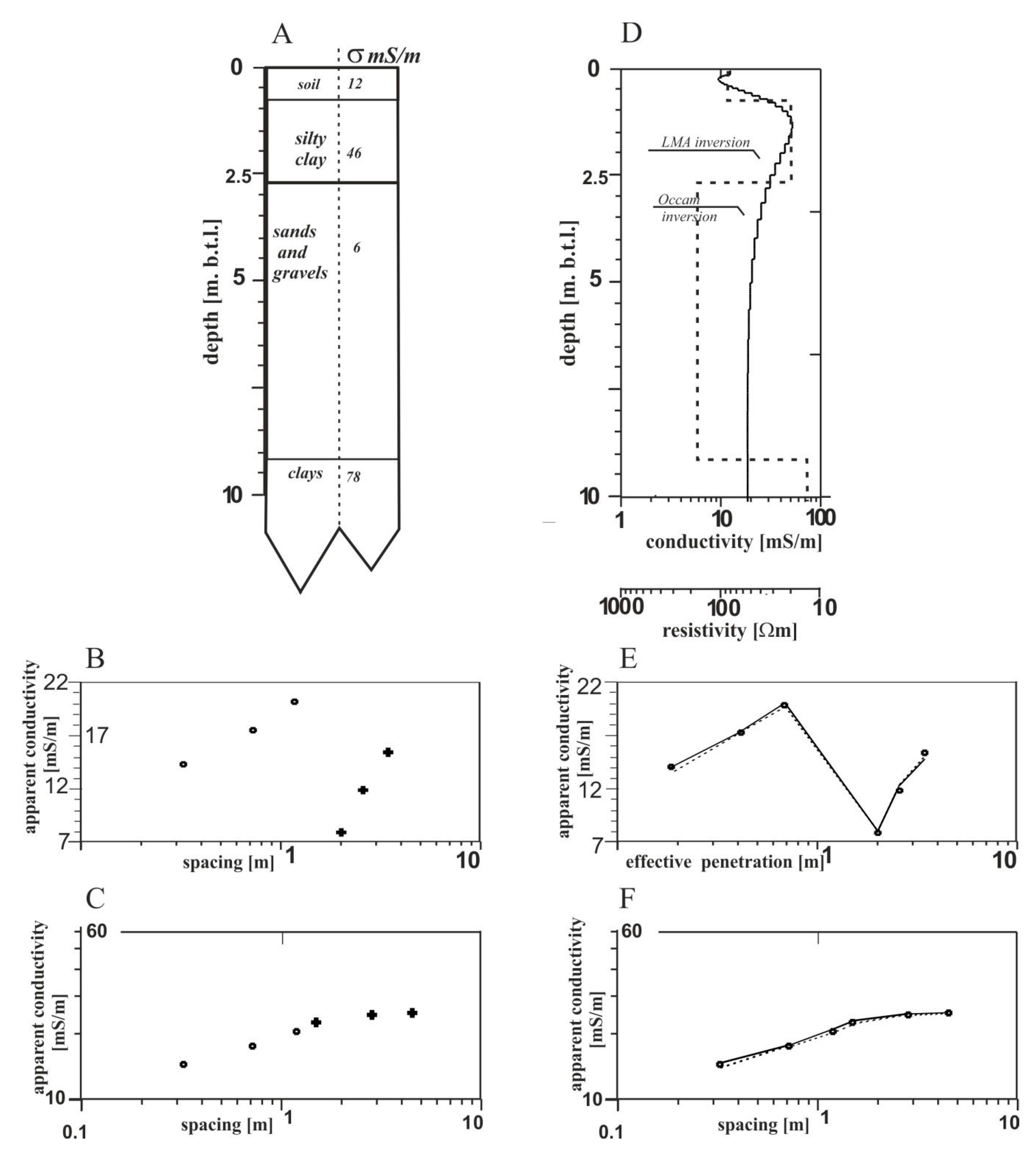
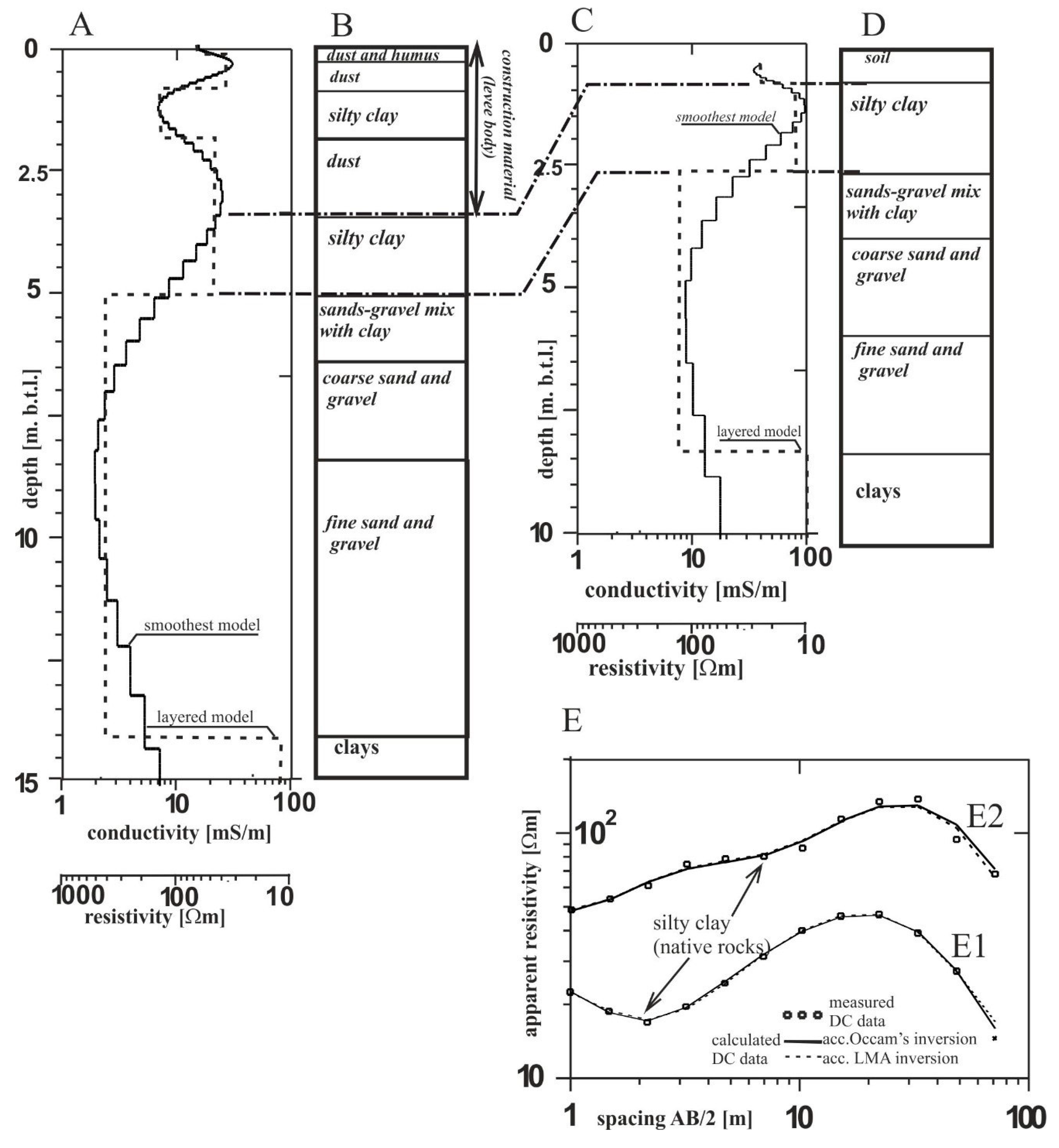
). ). The arrows on E show the influence of the silty clay layer on the DC sounding curves made on the levee crown (no. 4) and on the landward side (no. 5).
). The arrows on E show the influence of the silty clay layer on the DC sounding curves made on the levee crown (no. 4) and on the landward side (no. 5).
). The arrows on E show the influence of the silty clay layer on the DC sounding curves made on the levee crown (no. 4) and on the landward side (no. 5). ).
).
).
).


| Material | ρ [Ωm] | σ [mS/m] | Reference |
|---|---|---|---|
| Sand and gravels | 100−2500 | 0.4−10 | [15] |
| Clay | 1−100 | 10−1000 | |
| Loam | 5−50 | 20−200 | |
| Marls | 3−70 | 14−300 | |
| Sandstone | 500−5000 | 2−20 | |
| Soil | 10−800 | 1.25−100 | |
| Natural water | 1−100 | 10−1000 | [16] |
| Formation | Conductivity σ [mS/m] | Resistivity ρ [Ωm] | Frequency [kHz] | Skin Depth δ [m] | Frequency [kHz] | Skin Depth δ [m] |
|---|---|---|---|---|---|---|
| Sand + gravel | 5 | 200 | 30 | ~41 | 10 | ~71 |
| Soil | 10 | 100 | 30 | ~28 | 10 | ~50 |
| Silty clays | 50 | 20 | 30 | ~13 | 10 | ~22 |
| Clays | 100 | 10 | 30 | ~9 | 10 | ~16 |
| Instrument | Configuration | Spacing [m] | Penetration Depth [m] |
|---|---|---|---|
| CMD Mini Explorer f = 30 kHz | HD | 0.32 | ~0.25 |
| 0.71 | ~0.5 | ||
| 1.18 | ~0.9 | ||
| VD | 0.32 | ~0.5 | |
| 0.71 | ~1.0 | ||
| 1.18 | ~1.8 | ||
| CMD Explorer f = 10 kHz | HD | 1.48 | ~1.1 |
| 2.82 | ~2.1 | ||
| 4.49 | ~3.5 | ||
| VD | 1.48 | ~2.2 | |
| 2.82 | ~4.2 | ||
| 4.49 | ~6.7 |
| No. | CMD MiniExplorer | No. | CMD Explorer 1 m above the Ground Surface | CMD Explorer on the Ground Surface | |||
|---|---|---|---|---|---|---|---|
| S (m) | σa (mS/m) | S (m) | σa (mS/m) | S (m) | σa (mS/m) | ||
| 1 | 0.32 | 14.1 | 1 | 1.48 | 7.9 | 1.48 | 21.5 |
| 3 | 0.71 | 16.8 | 2 | 2.82 | 11.7 | 2.82 | 23.3 |
| 3 | 1.18 | 19.5 | 3 | 4.49 | 14.9 | 4.49 | 24 |
© 2020 by the authors. Licensee MDPI, Basel, Switzerland. This article is an open access article distributed under the terms and conditions of the Creative Commons Attribution (CC BY) license (http://creativecommons.org/licenses/by/4.0/).
Share and Cite
Klityński, W.; Oryński, S.; Chau, N.D. The Potential Use of Ground Conductivity Meters to Identify the Location of Seepages—Case Study of the Maniów Levee near Krakow, Poland. Geosciences 2020, 10, 97. https://doi.org/10.3390/geosciences10030097
Klityński W, Oryński S, Chau ND. The Potential Use of Ground Conductivity Meters to Identify the Location of Seepages—Case Study of the Maniów Levee near Krakow, Poland. Geosciences. 2020; 10(3):97. https://doi.org/10.3390/geosciences10030097
Chicago/Turabian StyleKlityński, Wojciech, Szymon Oryński, and Nguyen Dinh Chau. 2020. "The Potential Use of Ground Conductivity Meters to Identify the Location of Seepages—Case Study of the Maniów Levee near Krakow, Poland" Geosciences 10, no. 3: 97. https://doi.org/10.3390/geosciences10030097
APA StyleKlityński, W., Oryński, S., & Chau, N. D. (2020). The Potential Use of Ground Conductivity Meters to Identify the Location of Seepages—Case Study of the Maniów Levee near Krakow, Poland. Geosciences, 10(3), 97. https://doi.org/10.3390/geosciences10030097