Abstract
The accurate identification of kinematic parameters is crucial for improving the positioning accuracy of industrial robots, particularly in advanced manufacturing and automation. However, limited measurement space in practical applications often leads to concentrated data, causing overfitting and unreliable parameter estimation when using traditional identification methods. To address these challenges, this study proposes an -regularization-based method to improve parameter identification accuracy by penalizing deviations from the nominal kinematic parameters. The regularization factor is determined using a k-fold cross-validation strategy, ensuring a balance between generalization and accuracy. The proposed method was validated on a six-axis industrial robot, with calibration performed in a constrained measurement space and verification conducted in an expanded workspace. Compared to traditional least-squares methods, which suffer from significant parameter deviations and overfitting, the proposed -regularized method effectively improves parameter estimation accuracy. Specifically, this method reduces the mean error from 3.461 mm to 0.399 mm, achieving an approximate 88% improvement compared to the error before calibration. These findings demonstrate the effectiveness of the proposed method in improving parameter identification and positioning accuracy under constrained measurement space.
1. Introduction
With the expanding scope of industrial robot applications [1] and the growing adoption of offline programming [2,3], the demand for high absolute positioning accuracy in industrial robots has increased significantly. However, positioning accuracy is often composed of various factors, such as kinematic parameter errors, joint compliance, backlash, and thermal expansion [4]. Among these, kinematic parameter errors are the most significant. These errors primarily arise from inaccuracies in manufacturing and assembly, leading to variations in link lengths, link offsets, joint angles, and link twists [5].
Kinematic calibration improves the robot’s positioning accuracy by identifying precise model parameters through optimization methods [6]. The techniques can be broadly categorized into two types depending on the need for pose information: open-loop and closed-loop methods [7]. The open-loop approach is implemented by using high-accuracy and large-range external measurement devices, such as laser trackers and optical trackers, to capture the pose information of the robot’s end-effector [8]. For example, Yuan and Sun [9] employed a laser tracker to simultaneously identify the kinematic and dynamic parameters of a seven-axis collaborative robot. Nubiola et al. [10] studied the calibration of industrial robots using an optical CMM and a laser tracker, respectively, and compared the accuracy and efficiency of the two devices. Zhang et al. [11] proposed a Bayesian modeling framework for the kinematic calibration of industrial robots and utilized a laser tracker to identify joint angle errors. This method allows for the collection of extensive and diverse measurement configurations over large spaces, providing sufficient excitation of the parameters and thereby ensuring high positioning accuracy. However, these large-scale measurement devices are typically costly and time-consuming to use. Alternatively, distance-based calibration methods have been explored, using sensors such as cable displacement sensors to measure distance information between points. Li et al. [12] used a drawstring displacement sensor to identify the kinematic parameters of an industrial robot and compared the performance of various algorithms. Gao et al. [13] utilized a cable displacement sensor to identify the kinematic parameters of a six-DOF ER20-C10 industrial robot, resulting in a significant reduction in distance errors. However, distance-based methods are limited by the accuracy of the sensors and cannot directly evaluate the robot’s positioning accuracy, as distance errors are not equivalent to position errors. Both position-based and distance-based methods require large measurement spaces, which are often unavailable in factory environments due to narrow layouts and limited robot motion ranges.
Closed-loop calibration methods eliminate the requirement for large measurement spaces and costly external devices by imposing specific motion constraints on the robot. Various types of constraints have been proposed for this purpose, including point constraints [14], point and distance constraints [15], distance and spherical constraints [16], and planar constraints [17,18]. These constraints establish fixed relationships between the robot’s tool and reference features, enabling accurate calibration. He et al. [14] proposed a calibration method for industrial robots based on multiple position constraints, utilizing the relative pose information of the robot’s tool to improve accuracy. Joubair and Bonev [17] developed a method for identifying non-kinematic parameters of six-axis industrial robots using multiple planar constraints. He et al. [15] performed kinematic calibration of a collaborative robot using position and distance constraints. In addition to these methods, some researchers have utilized non-contact sensors, such as laser displacement sensors and vision systems, in combination with constraints to perform robot calibration. Stepanova et al. [19] proposed an automatic self-contained calibration method for dual-arm industrial robots by utilizing cameras, force sensors, and planar constraints to calibrate kinematic parameters. Similarly, Wang et al. [20] proposed a vision-based method incorporating distance constraints, achieving a significant reduction in average positioning errors. Despite these advancements, many methods rely on rigidly fixing the robot’s tool to a specific point or surface, which can be challenging for servo-driven robots.
Originally developed for five-axis machine tools [21,22], the R-test has recently emerged as a promising technique for robot calibration [23,24]. It employs a combination of three or more displacement sensors to measure the three-dimensional position of a high-precision reference ball, efficiently identifying errors in both linear and rotary axes. Guo et al. [23] designed a non-contact R-test system using three laser displacement sensors to evaluate a robot’s position accuracy, though they did not extend it to kinematic calibration. Cui et al. [24] utilized the R-test to calibrate the kinematic parameters and the rotary axis angular positioning deviations of a six-axis industrial robot. However, the measurement range of the R-test is notably limited, as it is typically confined to within a few tens of millimeters. This restriction constrains the calibration space to a small area, which may lead to overfitting during the kinematic parameter identification of the robot, resulting in significant parameter errors and increased positioning errors when validated across larger workspaces.
To address these challenges, this study proposes an -regularization-based kinematic calibration method for limited measurement space. The kinematic error model of the robot is first established. Then, a regularization term is introduced to the kinematic parameters, and an iterative identification method for the regularized objective function is applied to estimate the parameters. The main contributions of this work include the following:
- Traditional least-squares methods for robot parameter identification often suffer from overfitting in constrained measurement spaces, resulting in poor positioning accuracy when applied to larger measurement spaces. The proposed -regularization framework addresses these issues by incorporating nominal kinematic parameters as prior knowledge. By introducing a penalty term based on deviations from nominal values, the method enhances the robustness of parameter identification and significantly improves the robot’s positioning accuracy.
- Unlike traditional calibration methods that rely on expensive equipment like laser trackers for large-space measurements, the proposed method utilizes a small-range measurement device, the R-test, in conjunction with the regularization technique for robot calibration. The experimental results show that the calibration accuracy achieved with the R-test is comparable to that obtained with a laser tracker in larger spaces. Additionally, the R-test allows for faster data collection and more convenient deployment, offering a practical and cost-effective solution for calibrating robots in complex industrial environments.
2. Kinematic Error Model
2.1. Forward Kinematic Modeling
Taking a six-degree-of-freedom Elite EC66 robot as an example, the coordinate systems of each link are established based on the Modified Denavit–Hartenberg (MD-H) convention [25], as illustrated in Figure 1. The transformation matrix between the coordinate systems of link and link i is defined as follows:
where is the link length, is the link twist, is the link offset, is the joint offset, and is the joint angle variable. The nominal kinematic parameters of the robot are shown in Table 1. By concatenating the transformation matrices for all six links, the pose of the robot’s flange at the sixth joint relative to the base coordinate system (BCS) can be expressed as follows:
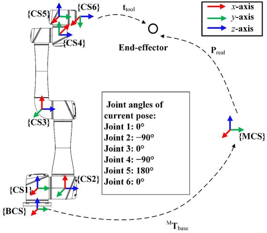
Figure 1.
Relationshipsbetween coordinate systems.

Table 1.
The nominal kinematic parameters.
In practical calibration, measurement devices are used to measure the position of the robot’s end-effector. After introducing the measurement coordinate system (MCS), the position of the end-effector in the MCS can be represented as follows:
where represents the translational offset of the tool relative to the sixth joint. The transformation matrix is defined as follows:
where is the rotation matrix, and represents the position of the BCS relative to the MCS. The predicted position can be written in a functional form as follows:
where represents the robot’s kinematic parameters; includes six parameters for BCS alignment and three for tool offset; denotes the joint configuration; and is the forward kinematics function.
For each joint configuration , the corresponding actual position of the robot is represented as , where . The error between the measured and predicted positions at pose k is expressed as follows:
Thus, the robot kinematic parameter identification problem can be formulated as the following nonlinear least-squares problem:
where denotes the Euclidean norm, and is the stacked error vector of N individual residuals.
2.2. Least-Squares Parameter Identification
For the nonlinear least-squares problem defined in Equation (7), Jacobian-based iterative methods, such as the Gauss–Newton algorithm [26,27] and the Levenberg–Marquardt algorithm [28], are widely applied to obtain the optimal estimate. The Jacobian matrix , which captures the sensitivity of the residuals to the parameters, is computed as follows:
This matrix contains the partial derivatives of the residuals with respect to the parameters and . Using the computed residuals and Jacobian matrix, the Gauss–Newton algorithm is applied to solve the linearized system and compute the parameter updates and . The update equations are given as follows:
To ensure that the Jacobian matrix maintains full rank during the parameter identification process, it is necessary to exclude redundant parameters that contribute to its singularity or near-singularity [29]. For example, in the case of the EC66 robot, when the axes of the 2nd, 3rd, and 4th joints are parallel or nearly parallel, the partial derivative matrix corresponding to the link offsets , , and becomes linearly dependent or nearly linearly dependent. This dependency results in a singular or near-singular Jacobian matrix, making it impossible to uniquely determine these parameters without additional constraints or parameter elimination. Specifically, parameters such as are excluded from the optimization and assigned nominal values. After computing the parameter updates, the kinematic parameters and system parameters are iteratively updated as follows:
where the process continues until a convergence criterion is satisfied.
The convergence of the Gauss–Newton algorithm used here is ensured under specific conditions tied to the kinematic parameter identification problem. Firstly, the forward kinematics function , built from the MD-H convention, is continuously differentiable due to its trigonometric and linear components, ensuring smoothness. Secondly, the Jacobian is full rank when the robot’s measurement poses avoid singularities (e.g., aligned joints or degenerate configurations), a condition we enforce by selecting diverse joint configurations and fixing redundant parameters as noted above. Thirdly, initializing and with nominal values (e.g., from factory settings or prior calibration) places the starting point near the true solution. Under these assumptions, the Gauss–Newton method exhibits local quadratic convergence, where the error decreases quadratically per iteration near the optimum, as the neglected second-order terms in the Hessian approximation become negligible [30].
This method performs well in scenarios with a large measurement space [31,32], enabling accurate calibration results. However, when the measurement range is limited, the reduced diversity of calibration poses may cause parameter overfitting, which degrades the robot’s positioning accuracy in larger workspaces.
3. -Regularization for Kinematic Parameter Identification
-regularization, also known as Tikhonov regularization, is widely recognized in statistics and mathematical modeling for stabilizing ill-posed problems [33,34] by introducing a penalty term to the objective function, effectively balancing data fidelity and solution simplicity. Unlike -regularization [35], which induces sparsity by setting some parameters to zero, -regularization ensures that all parameters contribute to the model, making it more stable. Therefore, -regularization is adopted in this paper to enhance the stability and accuracy of kinematic parameter identification. By imposing a penalty on deviations of the kinematic parameters from their nominal values, the estimates are encouraged to remain close to the design specifications. In contrast, the base and tool parameters, which lack strong prior constraints and may vary significantly with robot reconfiguration, are excluded from this regularization. Consequently, the regularized objective function is defined as follows:
where is the regularization parameter, represents the nominal kinematic parameters, and the regularization term is expressed as follows:
The regularization term itself, , penalizes the squared Euclidean distance between the estimated parameters and their nominal values, where is the norm of the parameter difference.
To facilitate the Gauss–Newton optimization method for solving the kinematic parameters under the constrained measurement space, it is necessary to compute the Jacobian matrix of the regularization term. Since is linear with respect to , the Jacobian matrix is given by the following:
where denotes the identity matrix whose size matches the number of kinematic parameters. Additionally, as the regularization term is independent of the base and tool parameters , the corresponding Jacobian matrix is zero. Thus, the full Jacobian matrix with respect to all parameters is expressed as follows:
where is a zero matrix matching the dimensions of . The total Jacobian matrix is then formed by combining the regularized Jacobian with the Jacobian of the residual error term:
The regularization parameter in the Jacobian matrix is crucial in balancing the influence of the regularization term [36]. To determine an appropriate value for , k-fold cross-validation is employed in this study [37]. By dividing the data into k folds and iteratively using one fold for validation and the remaining folds for training, this approach ensures that the selected generalizes well to unseen data. Additionally, k-fold cross-validation provides a robust estimate of the trade-off between model accuracy and overfitting.
After determining the Jacobian matrix and selecting the optimal , the regularized objective function is optimized iteratively. At each iteration, the parameter updates and are computed as follows:
Using these updates, the parameters and are refined iteratively according to the rule defined in Equation (10). The iterative process continues until a predefined convergence criterion is satisfied. The -regularization-based parameter identification method is summarized in Algorithm 1.
By incorporating -regularization, the proposed method mitigates parameter overfitting caused by the limited diversity of calibration poses in the constrained measurement space. The regularization term penalizes large deviations from the nominal values of the kinematic parameters, ensuring that the parameter estimates remain stable and robust.
| Algorithm 1 -regularization method for kinematic identification. |
|
4. Experimental Validation
To validate the proposed -regularized calibration method, parameter identification experiments are conducted on the EC66 industrial robot (Suzhou, China) within a limited measurement space. The performance of the method is compared with the traditional least-squares (LS) calibration approach, which does not incorporate regularization.
4.1. Setup and Data Collection
The experimental setup for robot calibration is shown in Figure 2a. The platform includes the EC66 six-axis collaborative robot and a non-contact R-test device. The robot has a payload capacity of 6 kg, a working radius of 914 mm, and a repeatability of 0.02 mm. A high-precision ceramic ball with a diameter of 50.7882 mm is attached to the robot’s flange as the calibration tool. In our previous work [38], we developed a custom non-contact R-test measurement device that uses five laser displacement sensors to precisely measure the center position of a ceramic ball. The device has a measurement range of and an accuracy of . In this paper, the R-test device is used to measure the ball’s center, which is positioned on the worktable. Despite the measurement range limitation of the R-test device, the tool’s motion space can still be effectively utilized by varying the robot’s orientations. This strategy allows for the collection of a diverse set of joint configurations and corresponding measured ball positions. Specifically, a total of 60 poses are collected, which collectively form the calibration set.
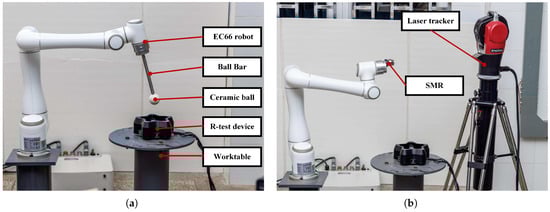
Figure 2.
Experimental setup for calibration-set and validation-set. (a) Experimental setup for calibration. (b) Experimental setup for validation.
To prepare for full kinematic parameter identification, a coarse estimation of the system parameters is performed using the hand–eye calibration method [39]. The errors obtained from this initial estimation are recorded as the before calibration errors. Building on this coarse estimation, the calibration set is used to identify all kinematic parameters. The optimal regularization coefficient is determined through 5-fold cross-validation, which provides a good balance between computational efficiency and model evaluation accuracy [40]. Candidate values of are sampled uniformly on a logarithmic scale from to , with a total of 50 candidates. The mean cross-validation error for each candidate is shown in Figure 3.To ensure robustness in this selection, we repeated this experiment three times, and although the optimal regularization coefficients varied slightly, they consistently remained in close proximity to 1.151. Based on the results, is selected as the optimal regularization factor, and parameter identification is performed using all the calibration data.The convergence criteria for these methods were consistently defined as either the objective function value falling below mm over 5 consecutive iterations or reaching a maximum iteration limit of 100.
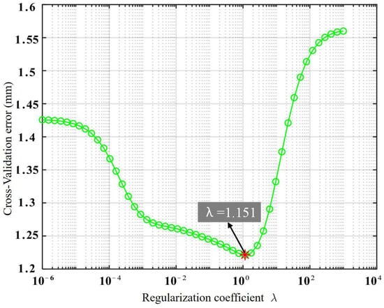
Figure 3.
Cross-validation error for different .
After calibration, an API laser tracker (Maryland, MD, USA) with a measurement accuracy of 10 is used to validate the accuracy of the identified parameters in a larger workspace, as shown in Figure 2b. To facilitate this validation process, the ceramic ball is replaced by a spherically mounted retroreflector (SMR) attached to the robot’s flange, enabling precise spatial measurements with the laser tracker. Subsequently, the base and tool parameters of the robot are obtained by the circle point analysis (CPA) method [41]. During the verification process, all methods are based on the same base and tool parameters. This consistency ensures that the errors observed in the verification results are primarily due to inaccuracies in the kinematic parameters. A mm cube is then chosen within the robot’s workspace, and 150 points are sampled using the Latin Hypercube Sampling method to form the validation set. The distributions of the calibration set and validation set are illustrated in Figure 4. During the data collection, the robot operates in a point-to-point mode. In this mode, the robot moves to each target point, waits for the data acquisition process to be completed, and then proceeds to the next point. Additionally, we randomly selected 60 points from the 150 validation points and applied the LS method for parameter identification to compare the calibration performance of the R-test with that achieved in a larger workspace.
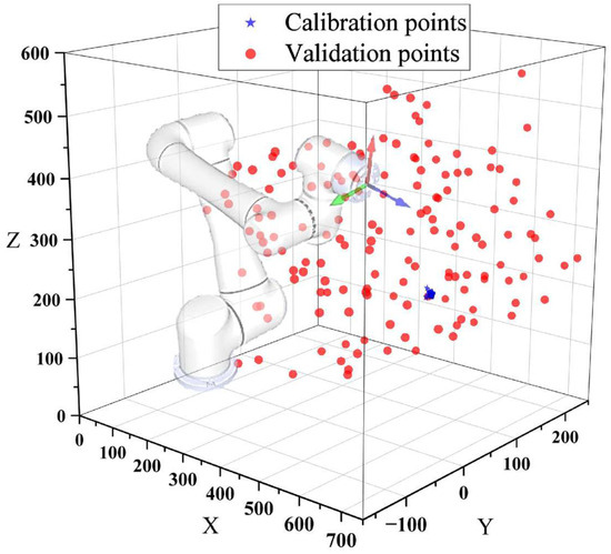
Figure 4.
Calibration-set and validation-set distributions.
To evaluate the performance of the methods, the position error at each pose is calculated as follows:
where , , and represent the differences between the measured and predicted positions along the x, y, and z axes, respectively.
4.2. Results and Discussion
Table 2 summarizes the calibration and validation errors for the Elite EC66 robot using R-test measurements within a constrained mm workspace for calibration and a mm workspace for validation. Three scenarios are compared: (i) before calibration, (ii) least squares with R-test (LS + R-test), and (iii) -regularized least squares with R-test (-Reg + R-test).
Table 2.
Comparison of calibration and validation errors with R-test.
For the calibration set, the error before calibration shows a mean error of 1.865 mm, a maximum error of 4.615 mm, and a standard deviation of 0.964 mm, reflecting notable kinematic inaccuracies. Both LS + R-test and -Reg + R-test markedly enhance accuracy in the calibration space. LS + R-test reduces the mean error by 89% to 0.206 mm, while -Reg + R-test yields a mean error of 0.213 mm, which represents an 88.6% reduction. The near-identical mean errors indicate effective fitting to the calibration data by both methods.
In the validation set, significant differences are observed between the two calibration methods. The LS + R-test method demonstrates poor generalization when applied to the larger workspace. The mean error increases by compared to before calibration, rising from to . Similarly, the maximum error increases by , reaching , compared to the initial value of . These results indicate that the LS + R-test method overfits the calibration data, leading to degraded performance in a larger workspace. In contrast, the -Reg + R-test method exhibits strong generalization capabilities, maintaining high accuracy across the larger workspace. The mean error and the maximum error are reduced to and , respectively, both representing reductions of compared to before calibration. Additionally, the standard deviation decreases by , indicating improved error stability across the validation set. The advantage of regularization lies in its penalty term, which constrains parameter deviations, preventing overfitting and enabling effective extrapolation despite the small calibration volume.
Table 3 presents the error results for the LS + Laser Tracker method, which was calibrated and validated within a mm workspace. A comparison between Table 2 and Table 3 demonstrates that the LS + Laser Tracker method establishes a strong baseline, with a validation mean error of 0.298 mm. The error distribution of the three methods in the validation space is shown in Figure 5. Notably, the -Reg + R-test method, calibrated within a substantially smaller mm workspace (8000 times smaller in volume), achieves a validation mean error of 0.399 mm, which is only 0.101 mm higher than the LS + Laser Tracker result. While the maximum error of -Reg + R-test (0.665 mm vs. 0.495 mm) exceeds that of LS + Laser Tracker by 0.170 mm, and its standard deviation (0.104 mm vs. 0.096 mm) is 0.008 mm greater, these differences are relatively modest given the significantly smaller calibration volume. In contrast, the LS + R-test method shows a considerably higher validation mean error of 7.278 mm, which is 6.980 mm worse than the LS + Laser Tracker method, highlighting its poor generalization performance under constrained measurement spaces.
Table 3.
Calibration and validation errors with the laser tracker.
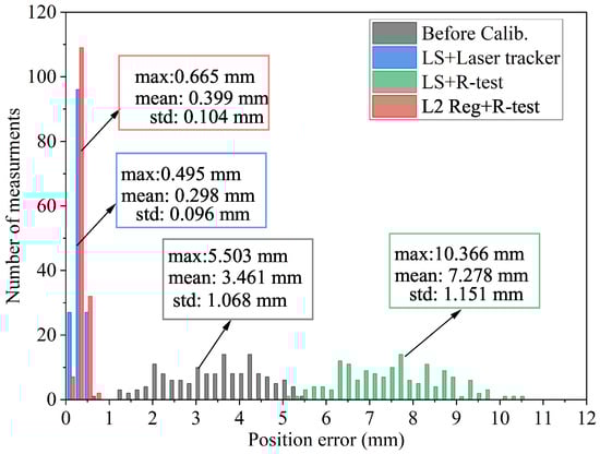
Figure 5.
Position Error distribution for different calibration methods.
An analysis of Table 4 reveals significant differences in the identified kinematic parameters across the LS + R-test, LS + Laser Tracker, and -Reg + R-test methods, reflecting their performance trends in Table 2 and Table 3. LS + R-test, calibrated in the mm space, exhibits large parameter deviations, e.g., mm and mm, far exceeding those of LS + Laser Tracker ( mm; mm) calibrated in the mm space. These large discrepancies suggest overfitting to the limited pose diversity in the small workspace, corroborated by LS + R-test’s validation mean error of 7.278 mm (Table 2). In contrast, -Reg + R-test parameters, e.g., mm and mm, closely resemble those of LS + Laser Tracker and deviate less from nominal values. This alignment is evident in its validation mean error of 0.399 mm, which is only 0.101 mm higher than LS + Laser Tracker’s 0.298 mm, despite the 8000-fold smaller calibration volume. The smaller deviations indicate that regularization curbs parameter over-adjustment, mitigating overfitting in constrained spaces and yielding more accurate kinematic estimates.
Table 4.
Comparison of identified parameters for LS and regularization.
Overall, the comparison demonstrates that the -regularized method achieves better kinematic parameter estimates in limited workspaces by balancing the trade-off between fitting the calibration data and maintaining parameter plausibility. It directly contributes to higher positioning accuracy in larger workspaces. This enhanced robustness and reduced sensitivity to measurement space limitations make the -regularized method an effective and reliable solution for kinematic calibration in constrained environments, offering a practical alternative to more costly and complex calibration setups.
5. Conclusions
This study presents an -regularized method for kinematic parameter identification in limited measurement spaces, leveraging nominal kinematic values as prior knowledge to construct a regularization term that penalizes large parameter deviations. Using R-test measurements within a constrained mm workspace, the approach was validated on a six-degree-of-freedom EC66 collaborative robot, demonstrating significant improvements in both parameter plausibility and positioning accuracy. The -regularized method mitigates overfitting caused by the limited calibration space inherent in R-test data collection, ensuring robust generalization to larger workspaces. The experimental results show that it consistently outperforms the traditional least-squares method with the R-test, achieving substantial reductions in positioning errors. In large-workspace validations ( mm), the mean error is reduced from 3.461 mm to 0.399 mm, representing an 88% reduction compared to the error before calibration. The proposed method provides a robust solution for robot calibration under limited measurement conditions with the R-test, ensuring accurate parameter identification and enhanced positioning performance. In future work, we will further investigate the applicability of the proposed method for enhancing pose accuracy in robotic calibration.
Author Contributions
Conceptualization, F.L. and G.G.; investigation, F.L.; methodology, F.L.; validation, F.L.; writing—original draft preparation, F.L.; writing—review and editing, F.L., G.G. and F.Z.; supervision, G.G. and J.N.; project administration and funding acquisition, G.G. and J.N. All authors have read and agreed to the published version of the manuscript.
Funding
This work was supported in part by the National Key R&D Program of China under grant 2023YFE0204700 and the National Natural Science Foundation of China under grants 52265001, 62273169, and 62303200.
Data Availability Statement
The datasets generated and/or analyzed during the current study are available from the corresponding author upon reasonable request.
Conflicts of Interest
The authors declare no conflicts of interest.
References
- Hou, M.; Cao, H.; Shi, J.; Guo, Y. An industry-oriented digital twin model for predicting posture-dependent FRFs of industrial robots. Mech. Syst. Signal Process. 2024, 212, 111251. [Google Scholar] [CrossRef]
- Weber, A.M.; Gambao, E.; Brunete, A. A Survey on Autonomous Offline Path Generation for Robot-Assisted Spraying Applications. Actuators 2023, 12, 403. [Google Scholar] [CrossRef]
- Rivera-Pinto, A.; Kildal, J.; Lazkano, E. Toward programming a collaborative robot by interacting with its digital twin in a mixed reality environment. Int. J. Hum. Interact. 2024, 40, 4745–4757. [Google Scholar] [CrossRef]
- Sigron, P.; Aschwanden, I.; Bambach, M. Compensation of Geometric, Backlash, and Thermal Drift Errors Using a Universal Industrial Robot Model. IEEE Trans. Autom. Sci. Eng. 2023, 21, 6615–6627. [Google Scholar] [CrossRef]
- Li, Z.; Li, S.; Luo, X. An overview of calibration technology of industrial robots. IEEE/CAA J. Autom. Sin. 2021, 8, 23–36. [Google Scholar] [CrossRef]
- Chen, X.; Zhan, Q. The kinematic calibration of an industrial robot with an improved beetle swarm optimization algorithm. IEEE Robot. Autom. Lett. 2022, 7, 4694–4701. [Google Scholar] [CrossRef]
- Hollerbach, J.M.; Wampler, C.W. The Calibration Index and Taxonomy for Robot Kinematic Calibration Methods. Int. J. Robot. Res. 1996, 15, 573–591. [Google Scholar] [CrossRef]
- Alam, M.M.; Ibaraki, S.; Fukuda, K.; Morita, S.; Usuki, H.; Otsuki, N.; Yoshioka, H. Inclusion of bidirectional angular positioning deviations in the kinematic model of a Six-DOF articulated robot for static volumetric error compensation. IEEE/ASME Trans. Mechatron. 2022, 27, 4339–4349. [Google Scholar] [CrossRef]
- Yuan, Y.; Sun, W. An Integrated Kinematic Calibration and Dynamic Identification Method with Only Static Measurements for Serial Robot. IEEE/ASME Trans. Mechatron. 2023, 28, 2762–2773. [Google Scholar] [CrossRef]
- Nubiola, A.; Slamani, M.A.; Joubair, A.; Bonev, I.A. Comparison of two calibration methods for a small industrial robot based on an optical CMM and a laser tracker. Robotica 2013, 32, 447–466. [Google Scholar] [CrossRef]
- Zhang, D.; Liang, H.; Li, X.; Jia, X.; Wang, F. Kinematic calibration of industrial robot using Bayesian modeling framework. Reliab. Eng. Syst. Saf. 2025, 253, 110543. [Google Scholar] [CrossRef]
- Li, Z.; Li, S.; Luo, X. Efficient industrial robot calibration via a novel unscented Kalman filter-incorporated variable step-size Levenberg–Marquardt algorithm. IEEE Trans. Instrum. Meas. 2023, 72, 2510012. [Google Scholar] [CrossRef]
- Gao, G.; Li, Y.; Liu, F.; Han, S. Kinematic calibration of industrial robots based on distance information using a hybrid identification method. Complexity 2021, 2021, 8874226. [Google Scholar] [CrossRef]
- He, S.; Ma, L.; Yan, C.; Lee, C.H.; Hu, P. Multiple location constraints based industrial robot kinematic parameter calibration and accuracy assessment. Int. J. Adv. Manuf. Technol. 2019, 102, 1037–1050. [Google Scholar] [CrossRef]
- He, J.; Gu, L.; Yang, G.; Feng, Y.; Chen, S.; Fang, Z. A local POE-based self-calibration method using position and distance constraints for collaborative robots. Robot. Comput.-Integr. Manuf. 2024, 86, 102685. [Google Scholar] [CrossRef]
- Joubair, A.; Bonev, I.A. Kinematic calibration of a six-axis serial robot using distance and sphere constraints. Int. J. Adv. Manuf. Technol. 2015, 77, 515–523. [Google Scholar] [CrossRef]
- Joubair, A.; Bonev, I.A. Non-kinematic calibration of a six-axis serial robot using planar constraints. Precis. Eng. 2015, 40, 325–333. [Google Scholar] [CrossRef]
- Besnard, S.; Khalil, W.; Garcia, G. Geometric calibration of robots using multiple plane constraints. In Advances in Robot Kinematics; Springer: Dordrecht, The Netherlands, 2000; pp. 61–70. [Google Scholar]
- Stepanova, K.; Rozlivek, J.; Puciow, F.; Krsek, P.; Pajdla, T.; Hoffmann, M. Automatic self-contained calibration of an industrial dual-arm robot with cameras using self-contact, planar constraints, and self-observation. Robot. Comput.-Integr. Manuf. 2022, 73, 102250. [Google Scholar] [CrossRef]
- Wang, R.; Wu, A.; Chen, X.; Wang, J. A point and distance constraint based 6R robot calibration method through machine vision. Robot. Comput.-Integr. Manuf. 2020, 65, 101959. [Google Scholar] [CrossRef]
- Weikert, S. R-Test, a New Device for Accuracy Measurements on Five Axis Machine Tools. CIRP Ann. 2004, 53, 429–432. [Google Scholar] [CrossRef]
- Ibaraki, S.; Onodera, K.; Jywe, W.Y.; Hsu, C.M.; Chang, Y.W. Experimental comparison of non-contact and tactile R-Test instruments in dynamic measurement. Int. J. Adv. Manuf. Technol. 2023, 128, 5277–5288. [Google Scholar] [CrossRef]
- Guo, Y.; Song, B.; Tang, X.; Zhou, X.; Jiang, Z. A calibration method of non-contact R-test for error measurement of industrial robots. Measurement 2021, 173, 108365. [Google Scholar] [CrossRef]
- Cui, T.; Ibaraki, S. Calibration of rotary axis angular positioning deviations in a six-axis robotic manipulator by using the R-Test. Int. J. Adv. Manuf. Technol. 2024, 134, 3845–3862. [Google Scholar] [CrossRef]
- Craig, J.J. Introduction to Robotics: Mechanics and Control, 2nd ed.; Addison-Wesley Longman Publishing Co., Inc.: Boston, MA, USA, 1989. [Google Scholar]
- Zhou, Y.; Chen, C.Y.; Tang, Y.; Wan, H.; Luo, J.; Yang, G.; Zhang, C. A Comprehensive On-Load Calibration Method for Industrial Robots Based on a Unified Kinetostatic Error Model and Gaussian Process Regression. IEEE Trans. Instrum. Meas. 2024, 73, 1003611. [Google Scholar] [CrossRef]
- Liu, F.; Gao, G.; Na, J.; Zhang, F. Kinematic Calibration for Serial Robots Based on a Vector Inner Product Error Model. IEEE Trans. Ind. Electron. 2024, 72, 2832–2841. [Google Scholar] [CrossRef]
- Liu, J.; Deng, Y.; Liu, Y.; Chen, L.; Hu, Z.; Wei, P.; Li, Z. A logistic-tent chaotic mapping Levenberg Marquardt algorithm for improving positioning accuracy of grinding robot. Sci. Rep. 2024, 14, 9649. [Google Scholar] [CrossRef]
- Zhang, Y.; Guo, J.; Li, X. Study on redundancy in robot kinematic parameter identification. IEEE Access 2022, 10, 60572–60584. [Google Scholar] [CrossRef]
- Nocedal, J.; Wright, S. Numerical Optimization; Springer Series in Operations Research and Financial Engineering; Springer: New York, NY, USA, 2006. [Google Scholar]
- Luo, J.; Chen, S.; Zhang, C.; Chen, C.Y.; Yang, G. Efficient Kinematic Calibration for Articulated Robot Based on Unit Dual Quaternion. IEEE Trans. Ind. Inform. 2023, 19, 11898–11909. [Google Scholar] [CrossRef]
- Sun, T.; Liu, C.; Lian, B.; Wang, P.; Song, Y. Calibration for Precision Kinematic Control of an Articulated Serial Robot. IEEE Trans. Ind. Electron. 2021, 68, 6000–6009. [Google Scholar] [CrossRef]
- Djennadi, S.; Shawagfeh, N.; Inc, M.; Osman, M.S.; Gómez-Aguilar, J.F.; Arqub, O.A. The Tikhonov regularization method for the inverse source problem of time fractional heat equation in the view of ABC-fractional technique. Phys. Scr. 2021, 96, 094006. [Google Scholar] [CrossRef]
- Li, M.; Wang, L.; Luo, C.; Wu, H. A new improved fractional Tikhonov regularization method for moving force identification. Structures 2024, 60, 105840. [Google Scholar] [CrossRef]
- De, S.; Doostan, A. Neural network training using L1-regularization and bi-fidelity data. J. Comput. Phys. 2022, 458, 111010. [Google Scholar] [CrossRef]
- Yuan, X.; Kong, L.; Zhang, Z.; Huang, G.; Xie, A.; Chen, G. Analysis of the influence of passive joints on kinematic calibration of parallel manipulators based on complete error model. Precis. Eng. 2024, 90, 56–70. [Google Scholar] [CrossRef]
- Ye, H.; Wu, J.; Huang, T. Kinematic calibration of over-constrained robot with geometric error and internal deformation. Mech. Mach. Theory 2023, 185, 105345. [Google Scholar] [CrossRef]
- Gao, G.; Kuang, L.; Liu, F.; Xing, Y.; Shi, Q. Modeling and Parameter Identification of a 3D Measurement System Based on Redundant Laser Range Sensors for Industrial Robots. Sensors 2023, 23, 1913. [Google Scholar] [CrossRef]
- Wu, L.; Ren, H. Finding the Kinematic Base Frame of a Robot by Hand-Eye Calibration Using 3D Position Data. IEEE Trans. Autom. Sci. Eng. 2017, 14, 314–324. [Google Scholar] [CrossRef]
- Kim, D.Y.; Kim, T.K.; Kim, K.; Hwang, J.H.; Kim, E. Mode Prediction and Adaptation for a Six-Wheeled Mobile Robot Capable of Curb-Crossing in Urban Environments. IEEE Access 2024, 12, 166474–166485. [Google Scholar] [CrossRef]
- Boby, R.A. Kinematic Identification of Industrial Robot Using End-Effector Mounted Monocular Camera Bypassing Measurement of 3-D Pose. IEEE/ASME Trans. Mechatron. 2022, 27, 383–394. [Google Scholar] [CrossRef]
Disclaimer/Publisher’s Note: The statements, opinions and data contained in all publications are solely those of the individual author(s) and contributor(s) and not of MDPI and/or the editor(s). MDPI and/or the editor(s) disclaim responsibility for any injury to people or property resulting from any ideas, methods, instructions or products referred to in the content. |
© 2025 by the authors. Licensee MDPI, Basel, Switzerland. This article is an open access article distributed under the terms and conditions of the Creative Commons Attribution (CC BY) license (https://creativecommons.org/licenses/by/4.0/).