Abstract
In the process industrial systems, flow control valves are deemed vital components that ensure the system’s safe operation. Hence, detecting faults in control valves is of significant importance. However, the stable operating conditions of flow control valves are prone to change, resulting in a decreased effectiveness of the conventional fault detection method. In this paper, an online fault detection approach considering the variable operating conditions of flow control valves is proposed. This approach is based on residual analysis, combining LightGBM online model with Seasonal and Trend decomposition using Loess (STL). LightGBM is a tree-based machine learning algorithm. In the proposed method, an online LightGBM is employed to establish and continuously update a flow prediction model for control valves, ensuring model accuracy during changes in operational conditions. Subsequently, STL decomposition is applied to the model’s residuals to capture the trend of residual changes, which is then transformed into a Health Index (HI) for evaluating the health level of the flow control valves. Finally, fault occurrences are detected based on the magnitude of the HI. We validate this approach using both simulated and real factory data. The experimental results demonstrate that the proposed method can promptly reflect the occurrence of faults through the HI.
1. Introduction
In process industrial systems, control valves are frequently employed as essential actuators, serving a pivotal role. The flow control valve is the most common type of control valve. Flow control valves precisely regulate the flow passing through them by adjusting the valve stem displacement and the pressure difference across the valve. Nevertheless, flow control valves are often mandated to operate in a variety of environmental conditions, which can include extreme factors like high temperatures, high pressures, corrosive media, and hazardous explosive zones [1]. In these challenging environments, control valves face issues such as leakage and viscosity effects, which can lead to unforeseeable production failures and safety hazards [2,3,4].
The industrial process is influenced by various factors, including changes in fluid properties, fluctuations in operating conditions, and equipment aging. These factors pose challenges for flow control valve fault detection. In the event of a flow control valve malfunction, the performance of the control loop is compromised, leading to challenges in regulating both the displacement of the valve stem and the magnitude of fluid flow within the pipeline. Many studies employ physical modeling [5,6], statistical analysis [7,8], and machine learning [9,10,11] approaches to detect faults in control valves. Zhang et al. [12] developed a graphical model capable of simultaneously detecting multiple faults while reducing dependence on statistical methods. Shi et al. [13] proposed a method based on Intrinsic Mode Functions (IMF) and one-dimensional WDenseNet for diagnosing internal leakage faults in directional control valves. Conti et al. [14] selected current, acoustic emission, and vibration signals as the most promising monitoring technique. They optimized the feature extraction and data fusion processes to detect early leakage faults in control valves.
Although there have been many research projects on control valves, the accuracy of fault detection using physics-based methods is affected by the uncertainty in industrial processes [15]. On the other hand, when it comes to statistical data and machine learning methods, the scarcity of labeled fault data compared to the vast amount of data from normal operation in industrial processes results in the problem of data imbalance, leading to low accuracy in fault detection methods [16]. In response to this issue, approaches to addressing the problem have been provided by methods based on data modeling and residual analysis. Residual-based stepwise attribute assessment methods have consistently held a pivotal and irreplaceable role in the field of fault detection. The most prominent advantage of the residual analysis stepwise attribute evaluation method is its independence from a substantial volume of fault data and the absence of a requirement for data specific to particular fault events [17].
The main emphasis in using residual analysis methods is on building models and assessing residuals. Therefore, it is crucial to address two key issues in this approach: how to quickly and accurately model the system and analyze residuals for effective fault detection. Heydarzadeh et al. [18] proposed a two-stage monitoring architecture for diagnosing actuator abnormalities. Initially, a model was established for fault-free processes using LS-SVM, followed by DWT analysis of the prediction model’s residuals to diagnose faults. Simani et al. [19] introduced a model-based dynamic system input–output control sensor fault detection and isolation method that leveraged analytical redundancy. This approach began with the construction of an industrial process model using standard identification techniques for variable error models. Subsequently, statistical tests were applied to the residuals for fault detection and isolation. Hu et al. [20] presented a current sensor fault diagnosis method that combines PSO-optimized residual generation with statistical residual assessment. It involved the development of a current sensor model based on charging principles, followed by statistical analysis of estimated residuals through Monte Carlo simulations to generate empirical residual thresholds, ensuring precise fault diagnosis for current sensors.
Although the residual analysis method has been widely applied in fault detection for various equipment, existing approaches for detecting faults in control valves still need to be revised. Firstly, factories often install a large number of control valves, each of which may operate under different conditions, and the operating conditions of individual control valves can change over time. Consequently, models trained offline often exhibit suboptimal performance when used online due to the diversity and variability of operating conditions. Secondly, when control valves experience gradual faults, the changes in residuals are often not prominent, making it challenging to accurately detect faults solely based on the magnitude of residuals. Therefore, it is essential to develop more precise and applicable methods for detecting faults in flow control valves that address these issues.
To address these challenges, it becomes imperative to establish online flow models for control valves that can adapt to varying operating conditions, thereby ensuring model accuracy. Given the need for high speed in online modeling, this research proposes a LightGBM-based approach for the online construction of control valve flow prediction models. This method not only ensures model accuracy but also boasts exceptional modeling speed. Subsequently, we employ the STL decomposition technique on the model’s flow residuals to capture their trends, which are then transformed into a health index (HI). Through the application of HI, we can not only detect the occurrence of faults but also assess the extent of gradual faults.
The contributions of this paper are as follows:
- An online LightGBM modeling method is proposed for constructing flow control valve models, and the residuals generated by this model are employed for control valve fault detection. This method is specifically tailored for large-scale and dynamically changing control valve systems and demonstrates higher modeling accuracy compared to traditional offline modeling methods.
- A residual analysis method based on STL decomposition is introduced. Through the decomposition of residual data from flow models, trend components are extracted and used to construct the HI metric for fault detection purposes.
The rest of this paper is organized as follows: Section 2 explains the fault detection framework using model residuals and the adoption of LightGBM modeling. Section 3 covers the dataset, along with presenting experimental results obtained using the proposed methods for flow control valve fault detection. Finally, in Section 4, we summarize and discuss the research findings.
2. Methods
2.1. Residual Analysis-Based Fault Detection
Equipment fault detection focuses on determining the presence of equipment faults that could impact the system’s operation. When equipment malfunctions, it exhibits significant differences from its normal state. It is possible to detect the occurrence of faults by identifying these differences. To enable fault detection, it is necessary to establish a model that represents the healthy operational state of the equipment. The residuals of the model, which signify the differences between predicted and observed values, encompass information about these variations. Therefore, effective fault detection is achievable through the analysis of residuals. This underscores the importance of establishing an accurate model, as the foundation of residual analysis relies on the precision of the model. The modeling phase involves learning the normal operational patterns of the system to establish a model that represents the system’s normal state [21].
Residuals are computed by feeding the operational data into the model and the actual system and then calculating the difference between the model’s output and the actual system’s output [22]. When provided with the model output and the actual system output y, the expression for residuals is as follows:
Through further analysis of residuals, changes in the residuals can be detected, indicating variations in the health status of the equipment. Considering the sequential characteristics of residual data, we employ the STL (Seasonal and Trend decomposition using Loess) decomposition method to analyze the residual data, aiming to extract potential fault or degradation trends. Compared to signal decomposition methods such as wavelet transform, STL decomposition can adapt to data with different periodicity and trends, without relying on the selection of basis functions, thus demonstrating better flexibility. For the original signal denoted as , the decomposition expression is as follows [23]:
where represents the trend component, represents the seasonal component, and denotes the remainder component. The STL approach involves a series of Loess (Locally Estimated Scatterplot Smoothing) smoothers used as an iterative non-parametric regression process. STL decomposition consists of two computational steps: an inner loop and an outer loop. The objective of the inner loop is to obtain the signal’s trend component, and its calculation steps are illustrated in Algorithm 1 [24], where and are the trend component and the seasonal component obtained from the kth decomposition, respectively.
Following the identification of residual trends, we transform this component into an indicator denoted as HI, confined within the interval of 0 to 1. As the equipment undergoes a transition from a state of normalcy to a faulty state, there is a gradual escalation in the residuals’ trend. Consequently, a mapping from [0, ) to (0,1] is established, effectively translating the residual trend into the HI metric. Under typical operating conditions, HI tends to stabilize around 1, but in the presence of a fault, it experiences a discernible decrease. The introduction of a square root operation to healthy residuals aims to mitigate fluctuations, thereby ensuring a more consistent HI during routine equipment operation. We define the HI as follows, where c is a regulation factor and is the trend component.
| Algorithm 1 STL decomposition inner loop. |
|
| Ensure: , |
2.2. LightGBM Algorithm
LightGBM [25] is an improved version of the Gradient Boosting Decision Tree (GBDT) model, incorporating techniques like one-sided gradient sampling and exclusive feature bundling. In this study, we have employed LightGBM to construct a flow prediction model for control valves. The operational principle of LightGBM involves iteratively adding and training new trees to fit the residuals from the previous iteration. Ultimately, LightGBM allocates a predictive value to each instance by summing the scores of all the leaf nodes.
Consider a training dataset containing n samples and m features, where , with representing the ith sample and representing the label value of the ith sample.
The prediction model expression for LightGBM is as follows:
where represents the ultimate prediction result for the input , K represents the number of trees, and denotes the result of input for the tth tree.
During each iteration, LightGBM constructs a decision tree, and for each training process, its objective function is as follows:
where is the loss function and is the regularization term. N represents the total number of leaf nodes, and is the score of each leaf node. and are controlling factors to avoid overfitting.
To simplify the loss function, consider a second-order Taylor expansion.
Make the following substitution:
The loss function can then be rewritten as follows:
As is a constant, it does not influence the optimization process and can be removed from the objective function, thus allowing the objective function to be rewritten as follows:
2.3. Online Learning Method
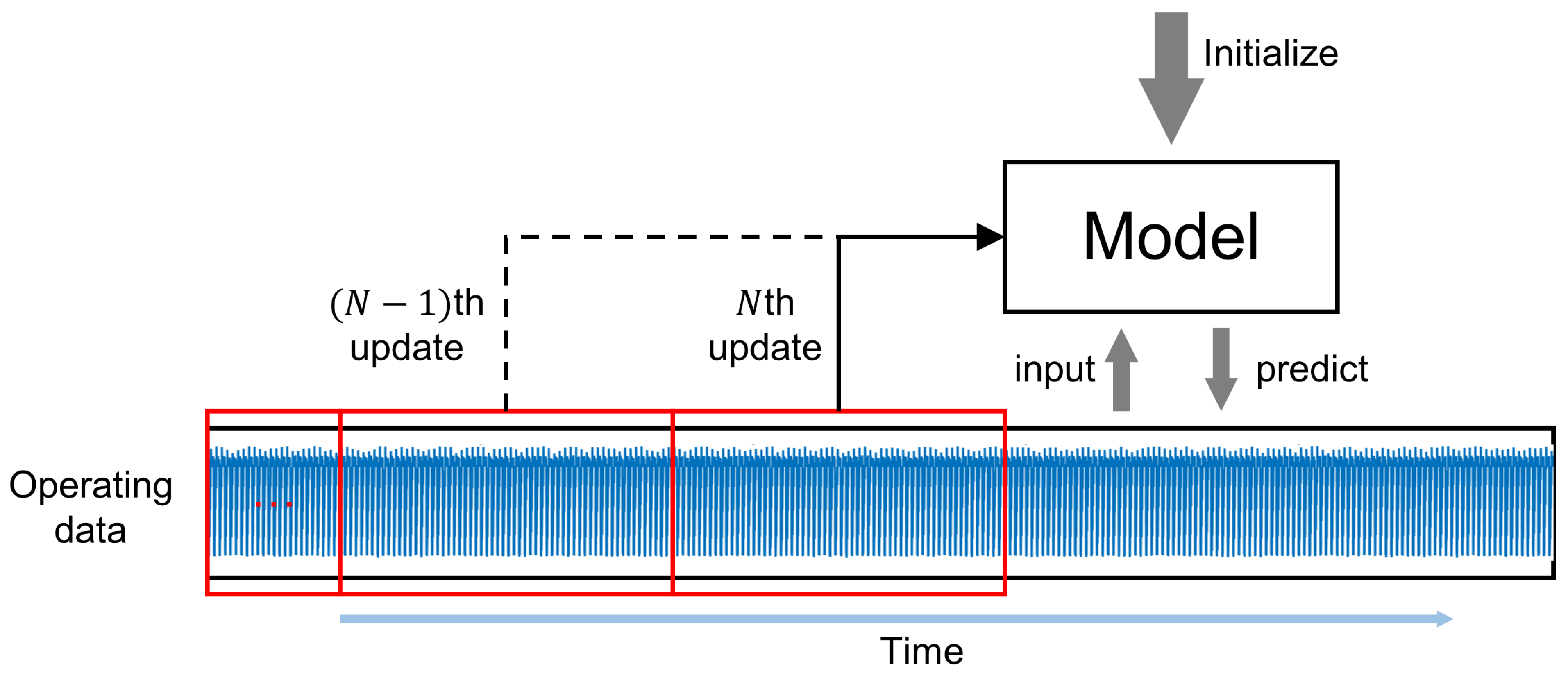
Online learning methods enable the model to dynamically adapt to changes in data by continuously updating it based on real-time data generated during system runtime. This approach enables the model to dynamically adapt to new information over time, providing a better reflection of the actual state of the system. Online learning is particularly valuable for handling real-time data and meeting the demands of dynamic changes in the system [26]. The process of online learning is illustrated in Figure 1. Online learning algorithms provide enhanced efficiency and scalability, especially in the context of large-scale machine learning tasks in practical data analysis applications. Online learning techniques are frequently applied in two primary scenarios. First, they enhance the efficiency and scalability of existing batch machine learning methods. Second, online learning algorithms are directly employed for the analysis of online streaming data [27].
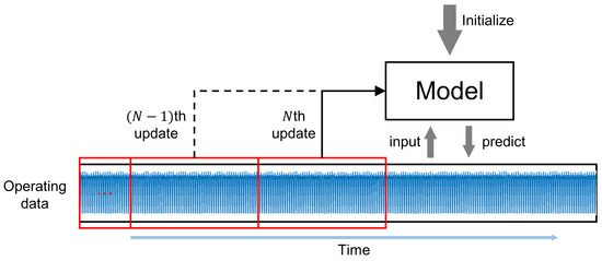
Figure 1.
The online learning process.
In real-world scenarios, numerous factories often have hundreds or even thousands of control valves, making traditional batch learning methods inefficient in terms of time and space costs. Furthermore, when the operational conditions of control valves change, the model needs to be retrained, which reduces the scalability of large-scale applications. However, online learning methods allow for updates on the existing model, minimizing the resource consumption associated with model retraining.
2.4. LightGBM-Based Residual Analysis for Online Fault Detection
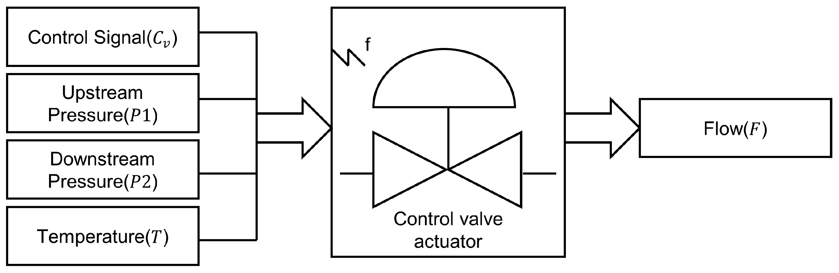
Precise flow control is one of the key functions of flow control valves [28], and many flow control valve faults can affect the effectiveness of flow control [29]. Therefore, it is possible to establish a flow model for control valves. When a fault occurs in the system, the detection of the fault can be achieved by monitoring changes in the flow model. The changes in the flow model can be reflected through flow residuals. By monitoring flow residuals, potential variations indicative of system faults can be identified, thereby enabling fault detection. The control valve flow equation is as follows [30]:
where Q is the flow, is the upstream pressure, is the downstream pressure, and is the discharge coefficient, which is related to fluid temperature and valve position. Based on the control valve’s flow equation, it is evident that the flow can be predicted using the valve’s upstream pressure, downstream pressure, valve position, and fluid temperature.
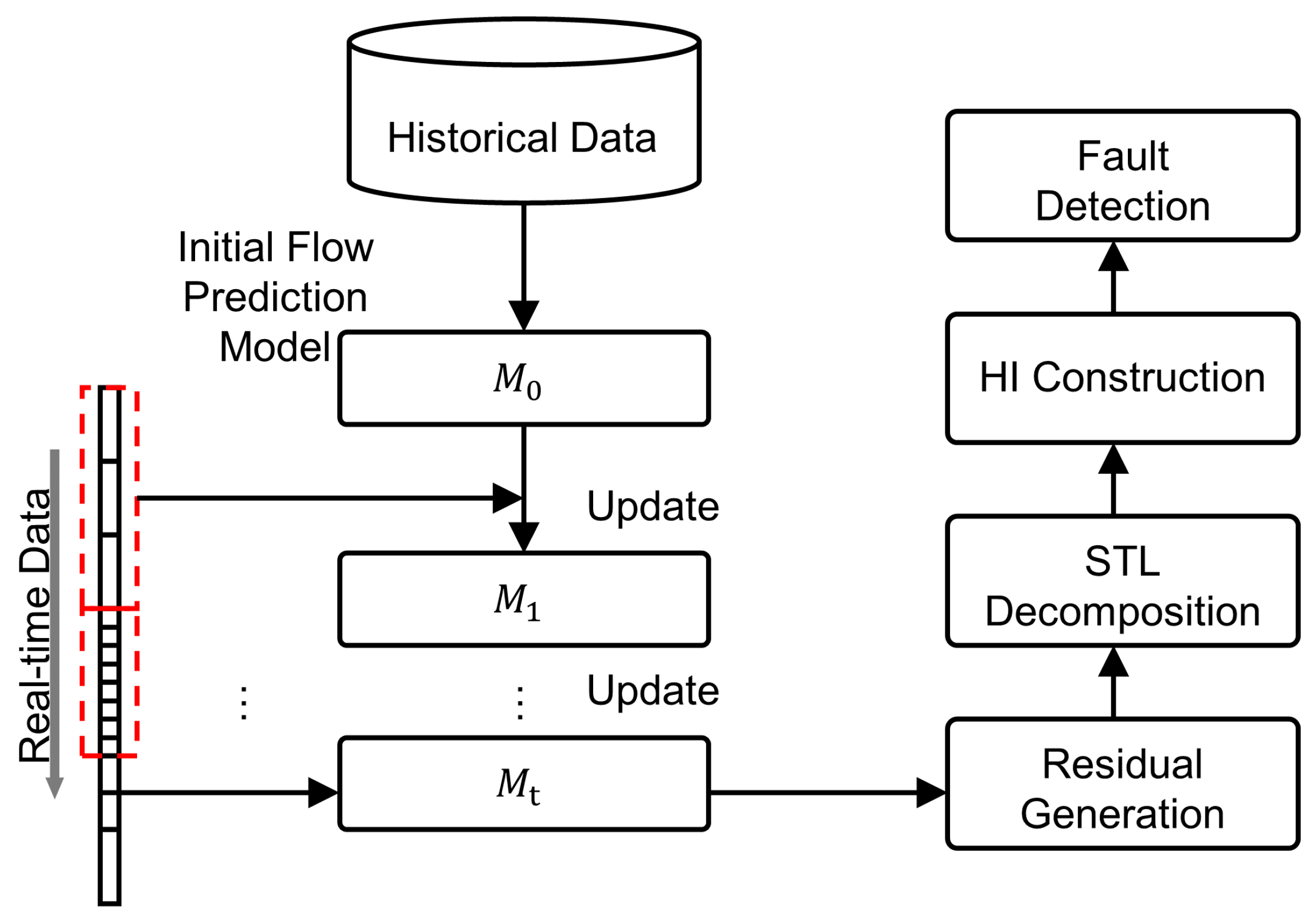
This method combines online learning with LightGBM and residual decomposition using STL to conduct fault detection. The online LightGBM can promptly update the model to adapt to changes in the operating conditions of the flow control valve, thereby reducing model prediction errors and improving the accuracy of fault detection. Simultaneously, the trend of residual changes obtained through STL decomposition provides an intuitive reflection of the health status changes in the flow control valve, enabling the detection of faults based on this information. The flowchart of the method is shown in Figure 2. To illustrate this method, an example is provided. At first, historical operational data from the control valve are gathered, encompassing parameters such as flow rate, pressure, fluid temperature, and valve position control signals. Due to the diversity of various types of physical quantities, data normalization is necessary. After normalization, the numerical range of the data is adjusted to be between 0 and 1. This facilitates the processing of different types of physical quantities on a unified scale, making them easier to compare and train. Subsequently, input features like upstream pressure, downstream pressure, fluid temperature, and valve position control signals are chosen, with flow rate serving as the target label. An initial flow rate prediction model is constructed through offline training using LightGBM. Assuming data are collected at a rate of one sample per second, and 600 training samples are needed to update the model, online updates are performed every 10 min using data from the previous 10 min of operation. When the model is employed to predict flow rate, the difference between the model’s predictions and the actual measurements results in flow residuals. Then, these residuals undergo STL decomposition. The trend components derived from this decomposition are then converted into an HI. Detection of fault occurrences is determined by the magnitude of the HI concerning a predetermined fault threshold. It is noted that the construction of HI is influenced by the tuning factor c. A smaller value of the tuning factor makes HI more sensitive to changes in residuals. Therefore, the selection of an appropriate fault threshold depends on the magnitude of c. If a fault threshold of 0.9 is set, any HI value below this threshold indicates the presence of a fault.

Figure 2.
The flow chart of the proposed fault detection method.
3. Experimental Analysis
3.1. Data Acquisition
The experiments were conducted using the DAMADICS (Development and Application of Methods for Actuator Diagnosis in Industrial Control Systems) [31] platform for simulation to obtain operational data of the control valve actuator. DAMADICS is a well-known benchmark for fault detection and isolation. It establishes simulation models based on the valves used in the Polish Lublin Sugar Plant production process and has developed a control valve actuator model library using MATLAB-SIMULINK. It effectively simulates typical fault modes of control valves. This platform can simulate 19 types of faults, and the simulated faults in control valves can be categorized into four types: 1. control valve body faults, 2. pneumatic servo motor faults, 3. positioner faults, and 4. external faults. Faults can also be classified as abrupt or gradual based on their temporal characteristics. During normal operation, the fault type is set to “f0”, indicating no fault. When simulating fault occurrences, the fault type is adjusted to correspond to the model fault. In this experiment, we simulate the operation of the control valve by providing periodic control signals and simulate the occurrence of valve faults by periodically varying the fault types. The DAMADICS model is depicted in Figure 3.
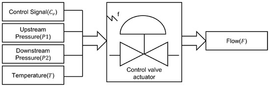
Figure 3.
General scheme of the DAMADICS model.
3.2. Online Learning Experiment
For methods based on model residuals, accuracy is crucial. If there is significant error in the modeling process, it may mistakenly diagnose a normally functioning system as having a fault. Within a factory setting, different control valves serve various purposes, leading to variations in their operating conditions. In such cases, if distinctions among different operating conditions are made, the model’s performance may be better when applied to data from varying conditions. Even when models are separately trained for each distinct operating condition, the effectiveness of the model may still be compromised, given that control valve conditions can change rapidly, and the model needs to adapt promptly.
From empirical observations, it is evident that if the data used during model training align closely with the operational characteristics of the target control valve, the predictive performance of the model on that specific control valve tends to be superior. Therefore, updating the model with new data in a timely manner, especially when the operating conditions of the control valve change, can significantly enhance model performance. To achieve this objective, we have employed an online learning approach to ensure that models for each control valve receive timely updates.
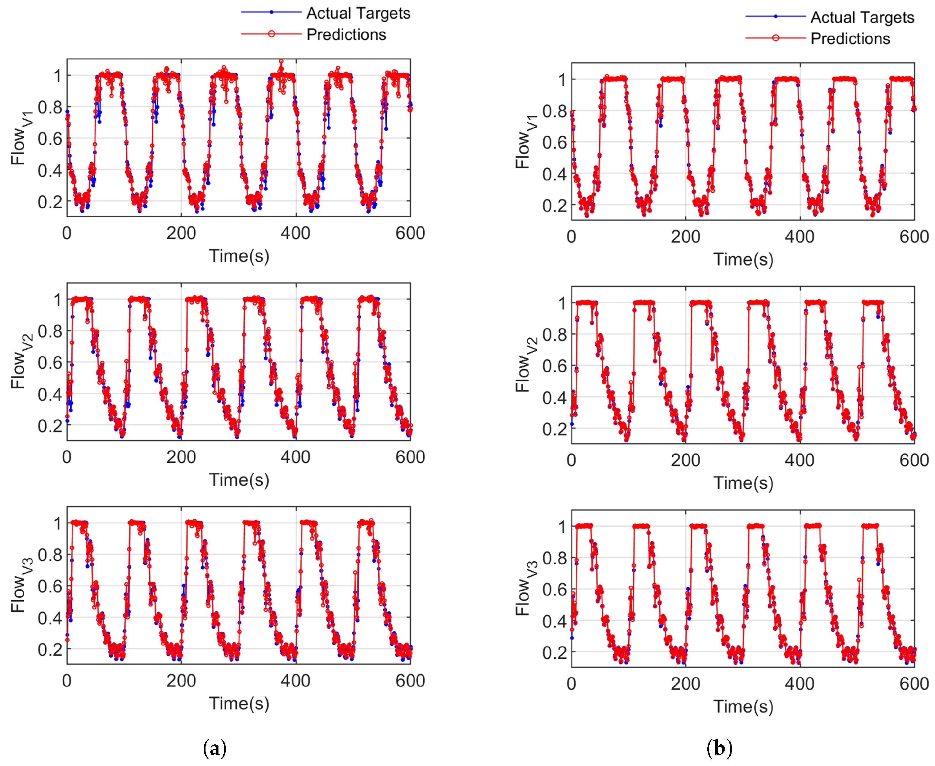
Through simulation experiments conducted on the DAMADICS platform, we generated operational data for control valves V1, V2, and V3 under three distinct operating conditions. Initially, these three different operating modes’ data were amalgamated to form the offline training dataset. Backpropagation (BP) neural network is a type of multilayer feedforward neural network trained using the backpropagation algorithm. By adjusting the weights within the network, BP neural networks aim to minimize the error between the actual output and the desired output. We employed a three-layer BP neural network to train our foundational flow prediction model using this dataset. Following this, we utilized data from various operating conditions to update the foundational flow prediction model, simulating the online learning process. The mean and variance of the flow data used for both offline and online training are presented in Table 1. We compared the performance of the offline model and the online model, assessing model performance using evaluation metrics such as Mean Squared Error (MSE), Mean Absolute Error (MAE), and Coefficient of Determination ().

Table 1.
The mean and variance of the dataset for offline BP and online BP.
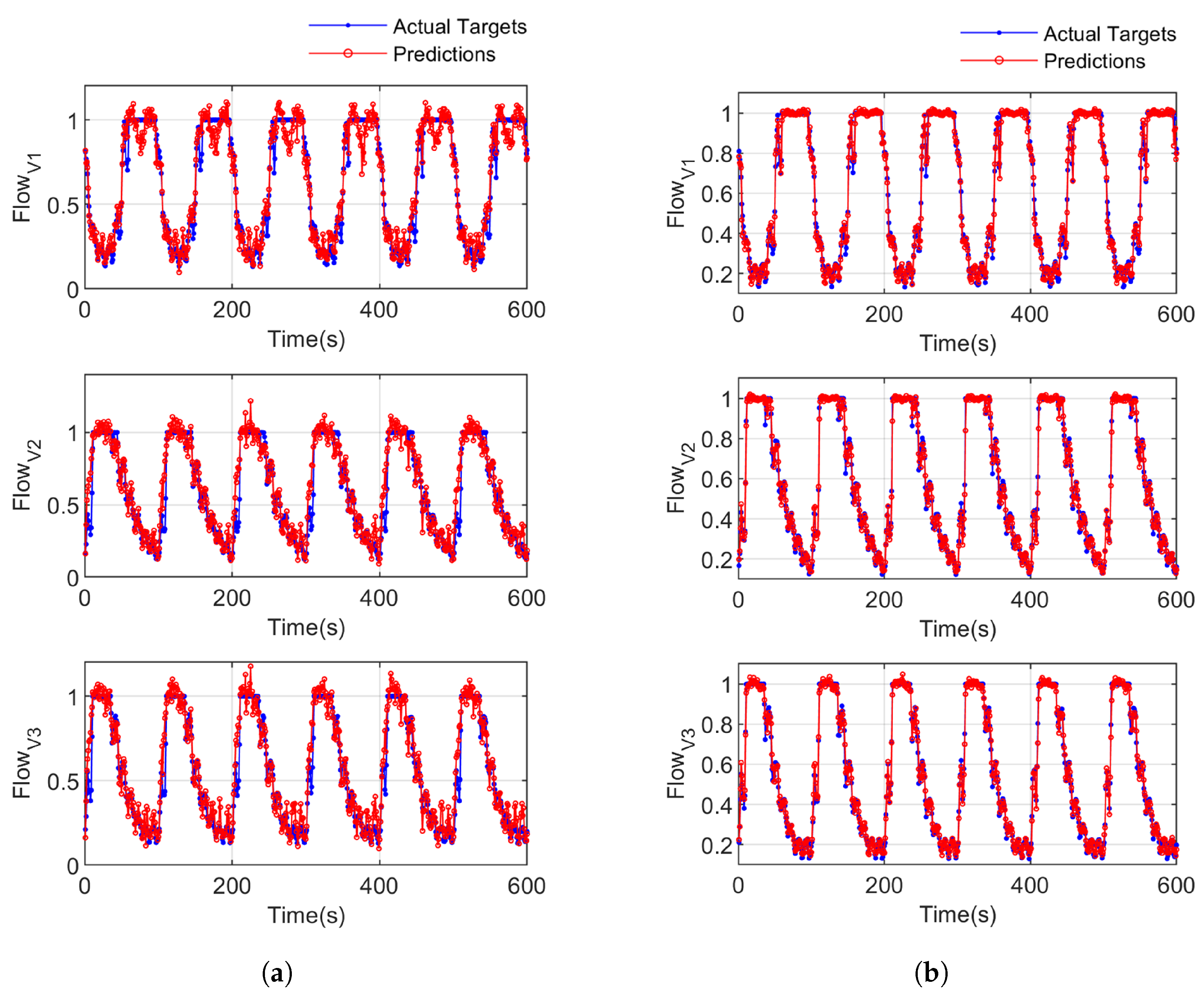
After comparing their ability to make predictions, it was clear that when dealing with data from control valves operating under three different conditions, the online model yielded better results compared to offline modeling, as shown in Figure 4 and Table 2. The offline model presents challenges in dealing with diverse data, potentially constraining the model’s generalization capability. This limitation becomes particularly evident when faced with various possible operational modes of control valves in real industrial scenarios. In contrast, the online model exhibits greater flexibility and adaptability, enabling timely model updates based on distinct data characteristics, ultimately resulting in superior predictive performance.
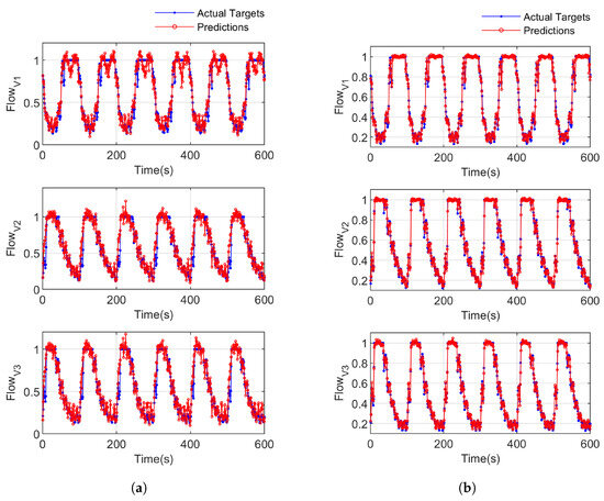
Figure 4.
The prediction performance of the backpropagation (BP) neural network: (a) offline model; (b) online model.
Table 2.
The performance comparison between offline BP and online BP.
In order to maintain optimal performance for the flow model, we employ an online learning approach to update the model. However, compared to the offline model, the online model entails a significant increase in time consumption due to the need for continuous model updates. Therefore, there is a requirement for fast online modeling techniques. Currently, commonly utilized models for online learning include neural networks and tree models.
Deep neural networks based on artificial neural networks exhibit significant advantages in terms of precision. However, they come with the drawback of lengthy training times, which is not advantageous for online modeling. Similar to neural networks, tree models possess robust scalability and the capability to update and train on existing models. Through ensemble learning, the combination of multiple decision tree weak learners forms a classification regression tree, preserving the tree model’s characteristic of fast modeling speed while demonstrating excellent performance in modeling precision. Therefore, in this context, we have chosen LightGBM, XGBoost, and BP neural networks as training models, comparing them in terms of model training speed and predictive performance. We have continued to employ the valve operation data from Section 3.2, applying the aforementioned modeling methods to valves operating under three different conditions.
Table 3 lists the prediction performance and required training time for BP, XGBoost, and LightGBM. The results show that LightGBM is very fast at modeling, beating both XGBoost and BP neural networks. When it comes to making predictions, LightGBM does as well as XGBoost and is even better than BP neural networks. For factories with lots of control valves, the shorter training time means using fewer resources.
Table 3.
The performance comparison of BP, XGBoost, and LightGBM.
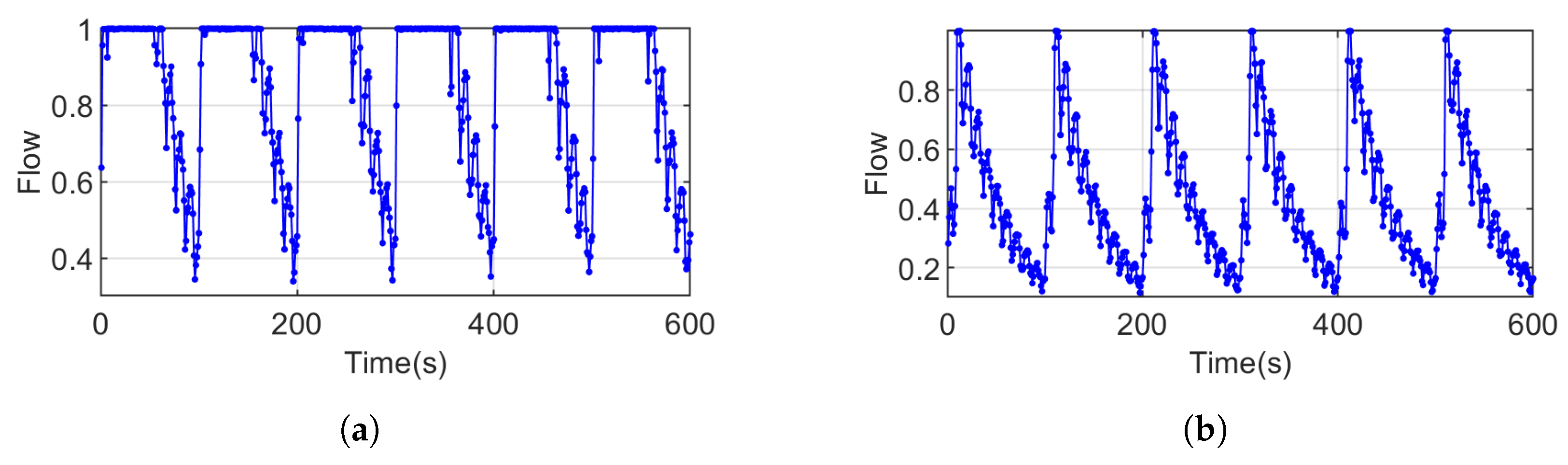
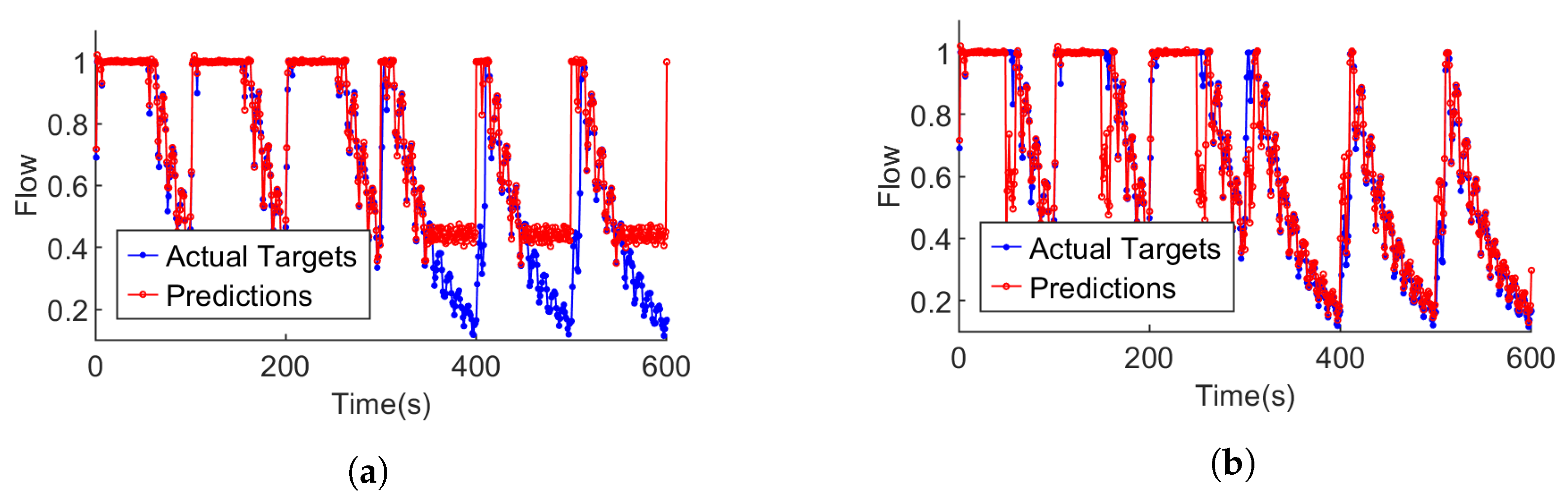
As previously mentioned, control valves are subject to variations in operating conditions while in use. In such cases, employing online modeling methods becomes crucial for timely model updates, thereby ensuring model performance. Figure 5 demonstrates the prediction effects of offline LightGBM and online LightGBM. To verify the effectiveness of the online modeling approach under varying operating conditions, we compared the prediction performance of offline and online models using data from changing operational scenarios. Figure 6 illustrates the variation in control valve flow before and after a change in operating conditions. We utilized data from before the change to establish the offline model and then updated the model online using data collected after the operational shift. Table 4 presents the prediction performance metrics for both offline and online models, including BP, XGBoost, and LightGBM, on the data collected after the change in conditions. Figure 7 visualizes the prediction results of the offline and online LightGBM models for the data reflecting these operational changes.
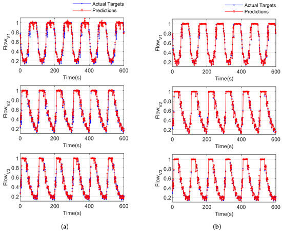
Figure 5.
The prediction performance of offline and online LightGBM: (a) offline; (b) online.
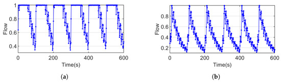
Figure 6.
Flow rate before and after operating condition changes: (a) before; (b) after.
Table 4.
Prediction performance of offline and online models under changing operating conditions.

Figure 7.
The prediction performance of LightGBM: (a) offline model; (b) online model.
3.3. Fault Detection Using Simulation Data
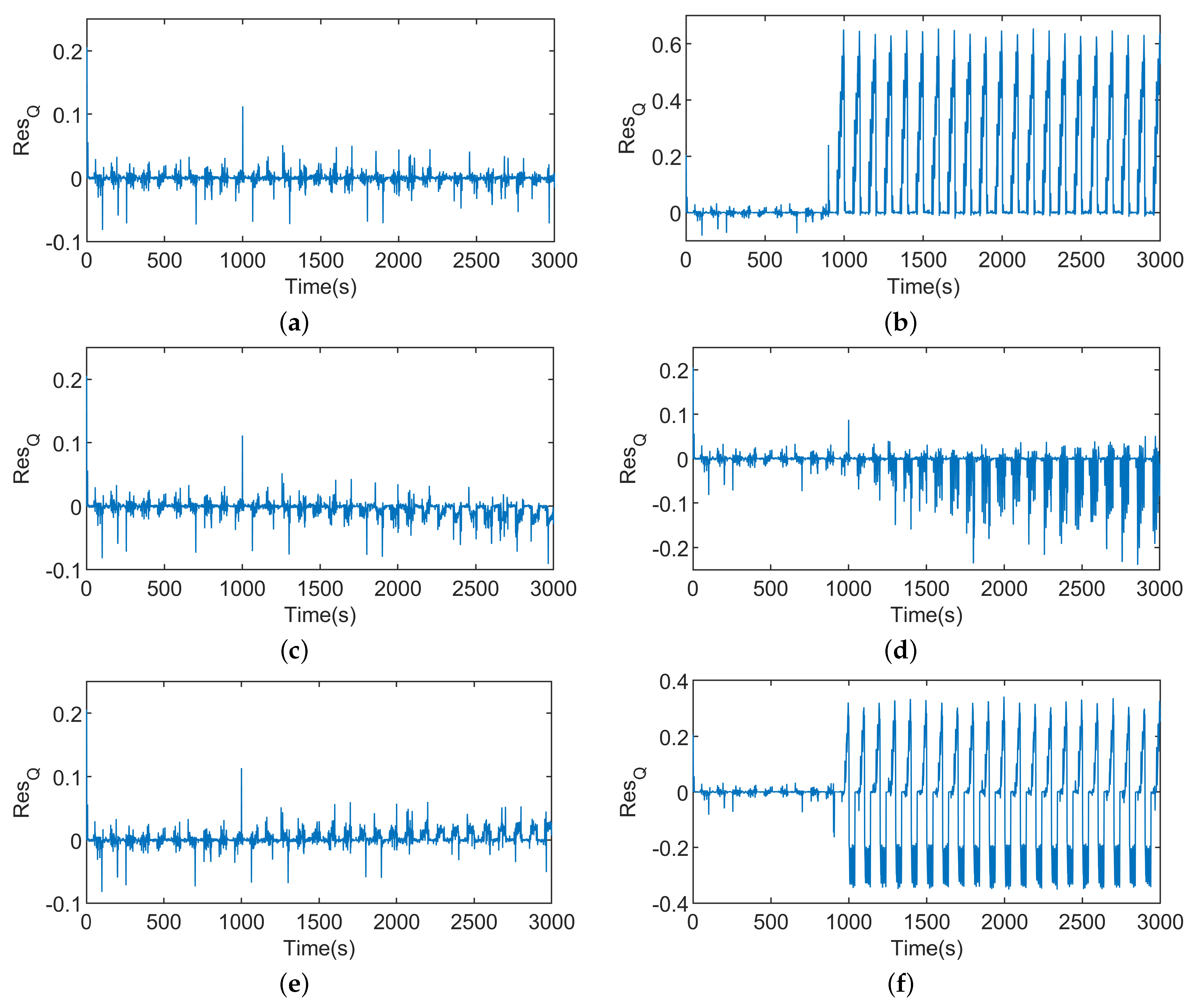
To validate the effectiveness of the proposed fault detection method, we conducted a series of simulation experiments using the DAMADICS platform to simulate five different types of control valve body faults. The fault labels and their descriptions are listed in Table 5. In these experiments, data were collected for each fault type, with each dataset comprising continuous data spanning 3000 s. The first 900 s of each dataset represent normal operating conditions, after which the faults were induced.
Table 5.
Fault labels and descriptions.
As shown in Figure 8, under normal conditions, the residual is minimal. However, when a fault occurs, a change in the residual is observed. It is worth noting that clogging and flashing exhibit the most significant changes in residuals, while sedimentation and internal leakage show relatively less pronounced changes in the early stages of the fault.
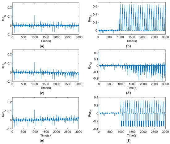
Figure 8.
Residuals in normal and 5 fault states. (a) Normal; (b) F1; (c) F2; (d) F3; (e) F4; (f) F5.
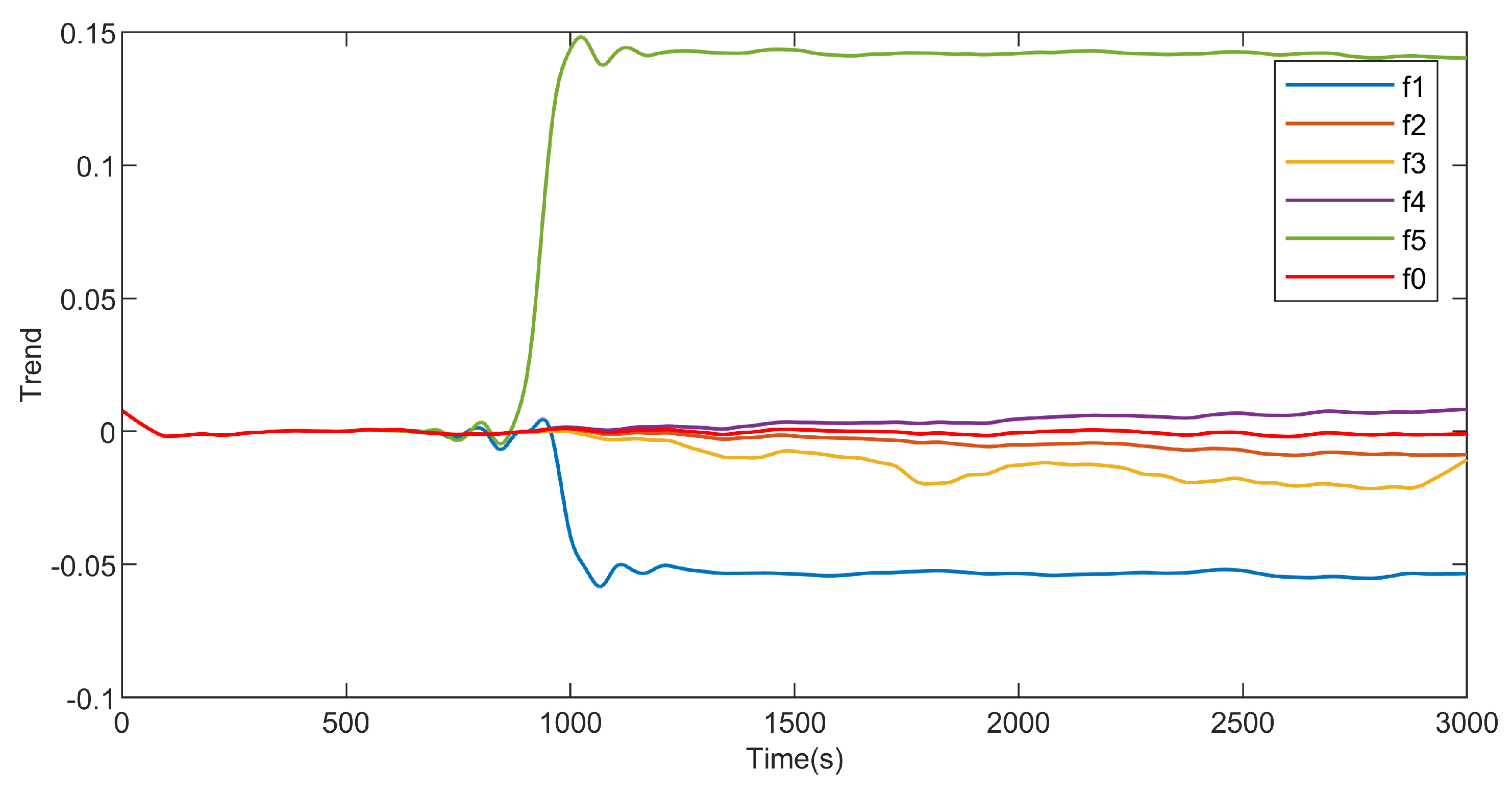
As shown in Figure 9, the residual trend components obtained through STL decomposition exhibit no significant variations under normal conditions. However, when sudden-failure-type faults occur, these trend components experience abrupt increases or decreases. In the case of gradual-failure-type faults, the trend components exhibit a slow-changing trend. By observing variations in the trend component, we can make preliminary assessments of the health status of a system or device. However, due to the diverse impacts of different types of faults on the trend component, theoretically, its numerical value can fluctuate indefinitely. This poses a challenge in directly describing the trend term numerically, as it becomes difficult to intuitively discern whether its changes have exceeded normal parameters. Consequently, a viable approach is to transform the trend term into an HI. By constraining the numerical value of the trend term within a range of 0 to 1, we can more conveniently utilize the HI value to assess changes in the health status and detect the occurrence of faults.

Figure 9.
Trend components after STL decomposition.
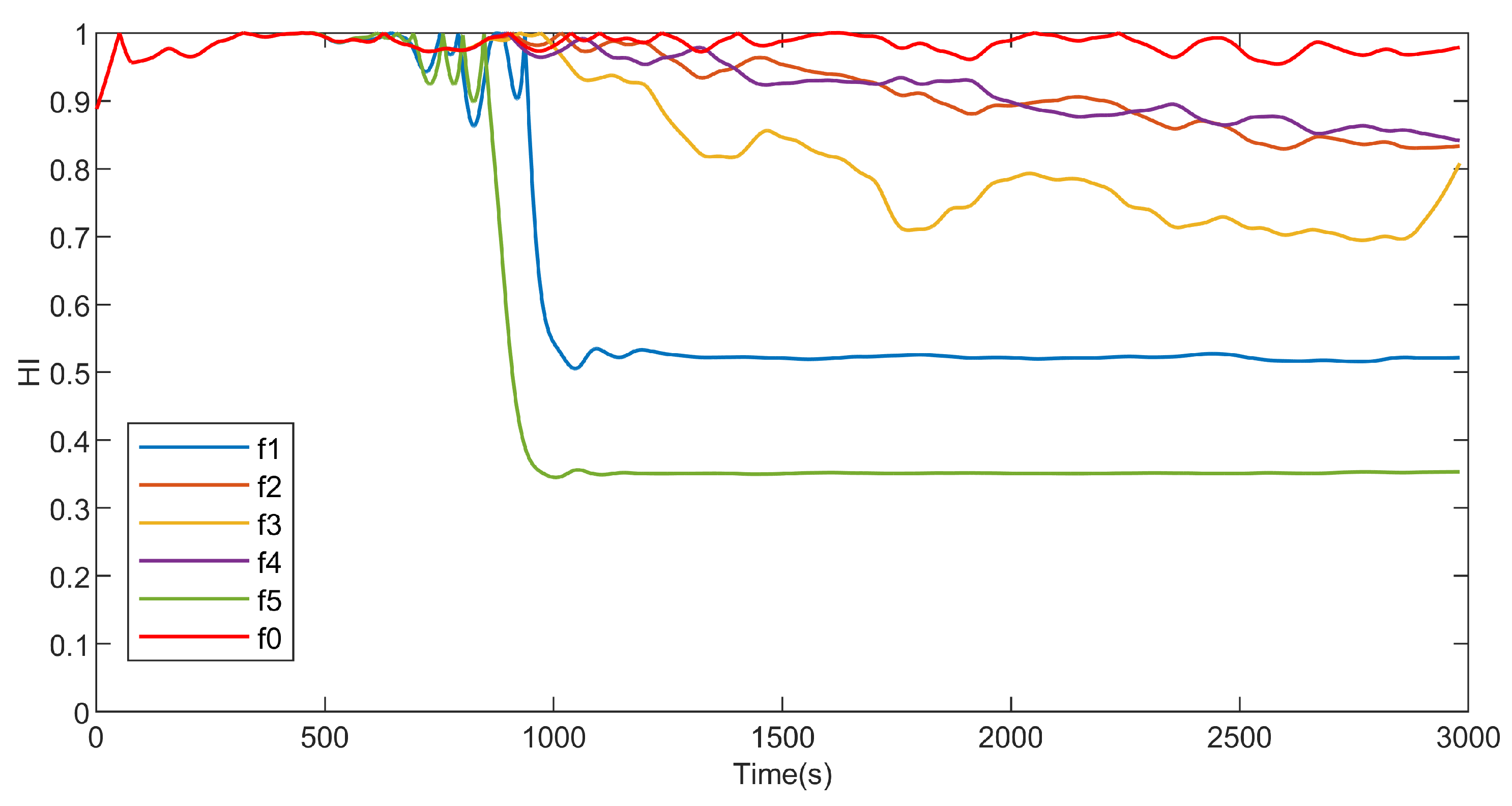
To accurately detect faults using HI, it is essential to establish a precise criterion, known as the fault threshold, for determining malfunctions. In the case of abrupt failures, where the transition from normal operation to a faulty state occurs instantaneously, selecting an appropriate threshold is relatively straightforward. However, for faults that deteriorate gradually, a clear boundary is essential to determine the point when equipment performance declines to an unacceptable level. Consequently, we have chosen to monitor changes in flow rate as our benchmark. Specifically, if the deviation in flow rate exceeds 0.5% compared to the normal flow rate under identical operating conditions, the equipment is deemed to have suffered a failure. The HI derived from the residual trend term is shown in Figure 10, where the tuning factor c is set to 0.2. The determination of the fault threshold relies on the variation of the HI during a fault occurrence. For this experiment, we set 0.85 as the critical threshold, and any HI value falling below 0.85 will indicate a system failure. At the 900 s mark, the abrupt occurrence of mutation faults, designated as f1 and f5, triggered a precipitous decline in the HI, pushing it below the critical threshold of 0.85. Concurrently, the gradual fault labeled f3 exhibited a more rapid evolution, culminating in system failure at 1773 s, coincident with a drop in HI to below 0.85. In contrast, gradual faults f2 and f4, owing to their sluggish progression, had not attained a failure state by the 3000-second benchmark, thereby maintaining their HIs above the 0.85 threshold. We compared the fault detection effectiveness of three online training models combined with STL decomposition to generate HI, as shown in Table 6.
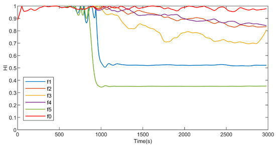
Figure 10.
HI in normal and 5 fault states.
Table 6.
Comparison of online model fault detection effectiveness.
3.4. Fault Detection Using True Factory Data
To validate the effectiveness of the proposed method in real industrial settings, we conducted experiments using the dataset from the Lublin Sugar Factory. This dataset encompasses operational data recorded from 29 October 2001 to 22 November 2001, with faults occurring on 30 October, 9 November, and 17 November. In this experiment, we selected 5000 data points from 29 October at 0:00 for offline model training. Figure 11 displays the upstream pressure, downstream pressure, temperature, and valve control signals used as inputs for the model, while Figure 2 shows the corresponding model output of flow rate.
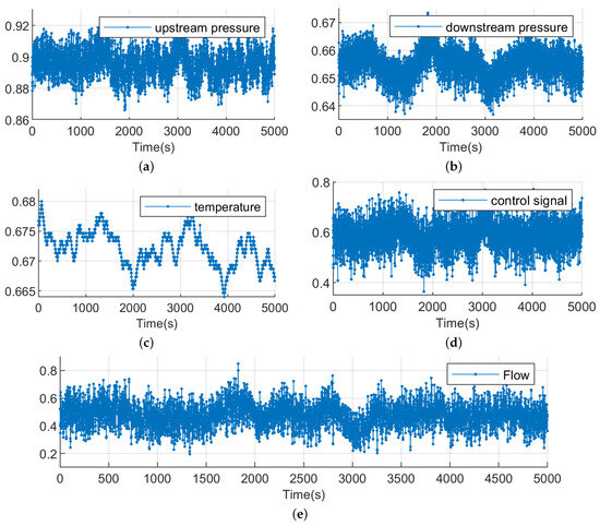
Figure 11.
Offline model training data: (a) upstream pressure; (b) downstream pressure; (c) temperature; (d) control signal; (e) flow.
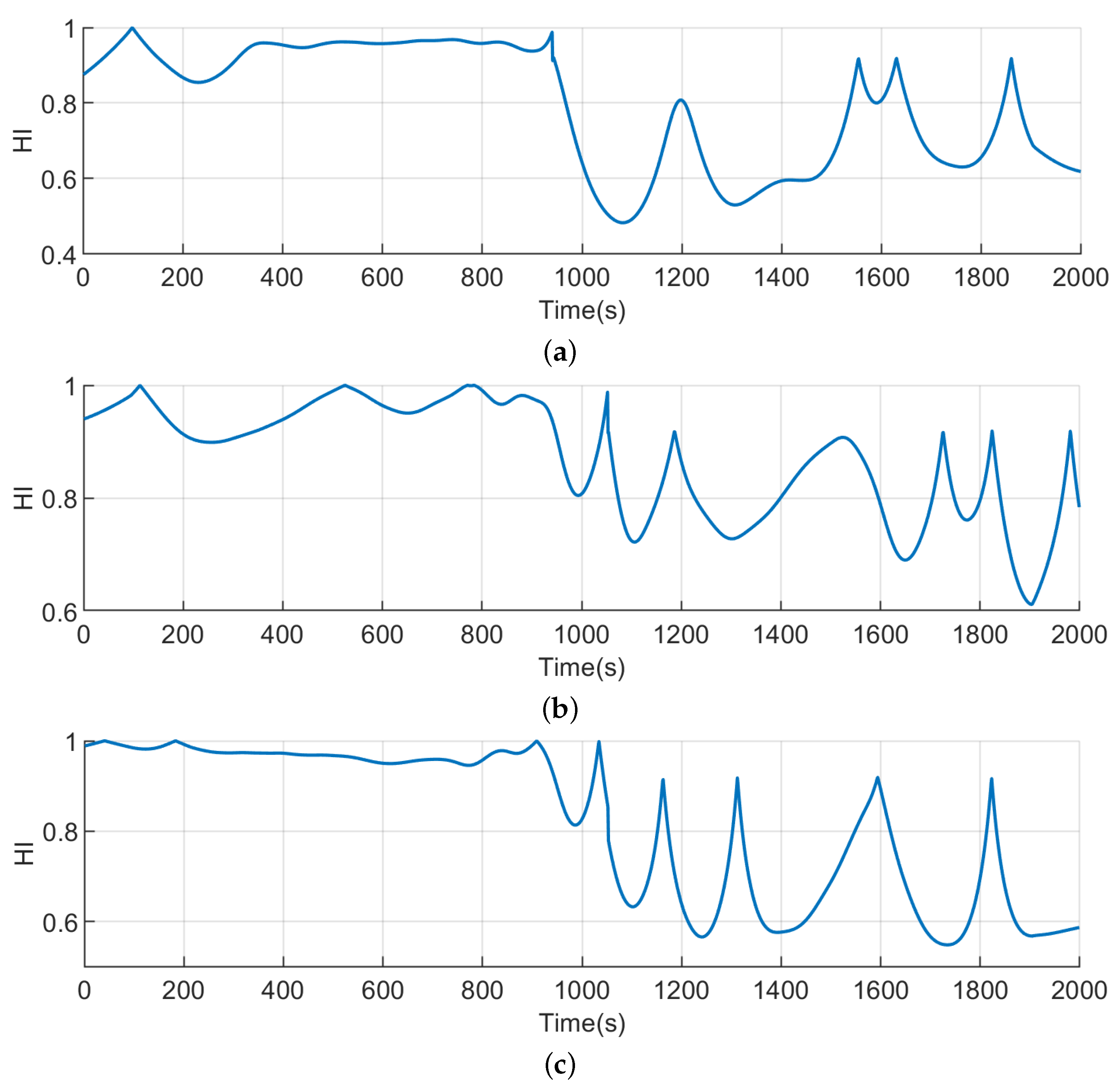
Afterwards, we updated the model using data collected before the occurrences of faults on 30 October, 9 November, and 17 November, respectively. On each fault day, the model was updated five times before the fault occurred, using 600 data points collected within a 10 min period for each update. Figure 12 illustrates the changes in HI during the occurrence of faults on three separate fault days. Evidently, when a fault occurs, there is a notable decrease in HI. In this context, we have set the adjustment factor for HI to 0.1, and the fault detection threshold remains at 0.85. The fault detection effectiveness is shown in Table 7.

Figure 12.
HIs using factory data: (a) 30 October; (b) 9 November; (c) 17 November.
Table 7.
Fault detection effectiveness on three fault days.
4. Conclusions
This paper proposed a fault detection method for the control valve based on online LightGBM model and residual STL decomposition. Initially, a control valve flow model is constructed using online LightGBM, demonstrating better adaptability to control valve conditions changes and higher accuracy than traditional offline models. Furthermore, LightGBM exhibits faster modeling capabilities than XGBoost and BP neural networks, making it more suitable for online learning requirements. Subsequently, the STL method decomposes the residual flow model, thus extracting trend components, which are then transformed into an HI for fault detection. The method is validated using DAMADICS simulation data and Lublin factory data, and it exhibits good performance in detecting abrupt and gradual fault types. The proposed method is influenced to some extent by the construction of the HI (Health Index) and the division of fault thresholds, leading to fluctuations in detection effectiveness when dealing with real factory data. Therefore, subsequent considerations should be given to alternative threshold determination methods to enhance the robustness of the detection approach.
Author Contributions
S.L. and T.Z.: data collection, analysis, interpretation of results, and draft manuscript preparation; D.Z.: supervision and revision of the manuscript. All authors have read and agreed to the published version of the manuscript.
Funding
This research was funded by the National Natural Science Foundation of China under Grant 62333010 and the National Key Research and Development Program of China No. 2020YFB1711203.
Data Availability Statement
The datasets used and/or analyzed during the current study are available from the corresponding author on reasonable request.
Conflicts of Interest
The authors declare that they have no conflicts of interest to report regarding the present study.
Abbreviations
The following abbreviations are used in this manuscript:
| DWT | Discrete Wavelet Transformation |
| HI | Health Index |
| LS-SVM | Least-Squares Support Vector Machine |
| BP | Back propagation |
| XGBoost | EXtreme Gradient Boosting |
| LightGBM | Light Gradient Boosting Machine |
| PSO | Particle Swarm Optimization |
| STL | Seasonal and Trend decomposition using Loess |
References
- Trunzer, E.; Weiß, I.; Folmer, J.; Schrüfer, C.; Vogel-Heuser, B.; Erben, S.; Unland, S.; Vermum, C. Failure mode classification for control valves for supporting data-driven fault detection. In Proceedings of the 2017 IEEE International Conference on Industrial Engineering and Engineering Management (IEEM), Singapore, 10–13 December 2017; IEEE: Piscataway, NJ, USA, 2017; pp. 2346–2350. [Google Scholar]
- Bolin, C.; Engeda, A. Analysis of flow-induced instability in a redesigned steam control valve. Appl. Therm. Eng. 2015, 83, 40–47. [Google Scholar] [CrossRef]
- Yang, Y.; Xiao, C.; Yang, Y. GRA and AHP analysis of pneumatic control valve failure in an LNG plant. Arab. J. Sci. Eng. 2021, 46, 1819–1830. [Google Scholar] [CrossRef]
- Han, X.; Jiang, J.; Xu, A.; Huang, X.; Pei, C.; Sun, Y. Fault detection of pneumatic control valves based on canonical variate analysis. IEEE Sens. J. 2021, 21, 13603–13615. [Google Scholar] [CrossRef]
- Manninen, T. Fault Simulator and Detection for a Process Control Valve. Ph.D. Thesis, Aalto University, Espoo, Finland, 2012. [Google Scholar]
- Wang, Y.; Wang, S.; Zhang, W.; Niu, Y. Research on Fault Modeling and Simulation of Electric Control Valve. In Proceedings of the 2021 33rd Chinese Control and Decision Conference (CCDC), Kunming, China, 22–24 May 2021; IEEE: Piscataway, NJ, USA, 2021; pp. 1290–1295. [Google Scholar]
- Kordestani, M.; Zanj, A.; Orchard, M.E.; Saif, M. A modular fault diagnosis and prognosis method for hydro-control valve system based on redundancy in multisensor data information. IEEE Trans. Reliab. 2018, 68, 330–341. [Google Scholar] [CrossRef]
- Helwig, N.; Pignanelli, E.; Schütze, A. Condition monitoring of a complex hydraulic system using multivariate statistics. In Proceedings of the 2015 IEEE International Instrumentation and Measurement Technology Conference (I2MTC) Proceedings, Pisa, Italy, 11–14 May 2015; IEEE: Piscataway, NJ, USA, 2015; pp. 210–215. [Google Scholar]
- Zhong, Q.; Xu, E.; Shi, Y.; Jia, T.; Ren, Y.; Yang, H.; Li, Y. Fault diagnosis of the hydraulic valve using a novel semi-supervised learning method based on multi-sensor information fusion. Mech. Syst. Signal Process. 2023, 189, 110093. [Google Scholar] [CrossRef]
- An, Z.; Cheng, L.; Guo, Y.; Ren, M.; Feng, W.; Sun, B.; Ling, J.; Chen, H.; Chen, W.; Luo, Y.; et al. A novel principal component analysis-informer model for fault prediction of nuclear valves. Machines 2022, 10, 240. [Google Scholar] [CrossRef]
- Venkata, S.K.; Rao, S. Fault detection of a flow control valve using vibration analysis and support vector machine. Electronics 2019, 8, 1062. [Google Scholar] [CrossRef]
- Zhang, Y.J.; Yuan, Y.; Hu, L.S. Fault Detection Based on Graph Model for Dead Zone of Steam Turbine Control Valve. Int. J. Control Autom. Syst. 2022, 20, 2759–2767. [Google Scholar] [CrossRef]
- Shi, C.; Ren, Y.; Tang, H.; Mupfukirei, L.R. A fault diagnosis method for an electro-hydraulic directional valve based on intrinsic mode functions and weighted densely connected convolutional networks. Meas. Sci. Technol. 2021, 32, 084015. [Google Scholar] [CrossRef]
- Conti, F.; Madeo, F.; Boiano, A.; Tarabini, M. Electrical and mechanical data fusion for hydraulic valve leakage diagnosis. Meas. Sci. Technol. 2023, 34, 044011. [Google Scholar] [CrossRef]
- Xu, Y.; Sun, Y.; Wan, J.; Liu, X.; Song, Z. Industrial big data for fault diagnosis: Taxonomy, review, and applications. IEEE Access 2017, 5, 17368–17380. [Google Scholar] [CrossRef]
- Liu, J. A minority oversampling approach for fault detection with heterogeneous imbalanced data. Expert Syst. Appl. 2021, 184, 115492. [Google Scholar] [CrossRef]
- Ranasinghe, K.; Sabatini, R.; Gardi, A.; Bijjahalli, S.; Kapoor, R.; Fahey, T.; Thangavel, K. Advances in Integrated System Health Management for mission-essential and safety-critical aerospace applications. Prog. Aerosp. Sci. 2022, 128, 100758. [Google Scholar] [CrossRef]
- Heydarzadeh, M.; Nourani, M. A two-stage fault detection and isolation platform for industrial systems using residual evaluation. IEEE Trans. Instrum. Meas. 2016, 65, 2424–2432. [Google Scholar] [CrossRef]
- Simani, S.; Fantuzzi, C.; Beghelli, S. Diagnosis techniques for sensor faults of industrial processes. IEEE Trans. Control Syst. Technol. 2000, 8, 848–855. [Google Scholar] [CrossRef]
- Hu, J.; Bian, X.; Wei, Z.; Li, J.; He, H. Residual statistics-based current sensor fault diagnosis for smart battery management. IEEE J. Emerg. Sel. Top. Power Electron. 2021, 10, 2435–2444. [Google Scholar] [CrossRef]
- Medjaher, K.; Zerhouni, N. Residual-based failure prognostic in dynamic systems. IFAC Proc. Vol. 2009, 42, 716–721. [Google Scholar] [CrossRef]
- Angelov, P.; Giglio, V.; Guardiola, C.; Lughofer, E.; Lujan, J. An approach to model-based fault detection in industrial measurement systems with application to engine test benches. Meas. Sci. Technol. 2006, 17, 1809. [Google Scholar] [CrossRef]
- Chae, J.; Thom, D.; Bosch, H.; Jang, Y.; Maciejewski, R.; Ebert, D.S.; Ertl, T. Spatiotemporal social media analytics for abnormal event detection and examination using seasonal-trend decomposition. In Proceedings of the 2012 IEEE Conference on Visual Analytics Science and Technology (VAST), Seattle, WA, USA, 14–19 October 2012; IEEE: Piscataway, NJ, USA, 2012; pp. 143–152. [Google Scholar]
- Bergmeir, C.; Hyndman, R.J.; Benítez, J.M. Bagging exponential smoothing methods using STL decomposition and Box–Cox transformation. Int. J. Forecast. 2016, 32, 303–312. [Google Scholar] [CrossRef]
- Ke, G.; Meng, Q.; Finley, T.; Wang, T.; Chen, W.; Ma, W.; Ye, Q.; Liu, T.Y. Lightgbm: A highly efficient gradient boosting decision tree. Adv. Neural Inf. Process. Syst. 2017, 30. [Google Scholar]
- Zhao, T.; Pan, S.; Gao, W.; Qing, Z.; Yang, X.; Wang, J. Extreme learning machine-based spherical harmonic for fast ionospheric delay modeling. J. Atmos. Sol.-Terr. Phys. 2021, 216, 105590. [Google Scholar] [CrossRef]
- Hoi, S.C.; Sahoo, D.; Lu, J.; Zhao, P. Online learning: A comprehensive survey. Neurocomputing 2021, 459, 249–289. [Google Scholar] [CrossRef]
- Wang, B.; Liu, H.; Hao, Y.; Quan, L.; Li, Y.; Zhao, B. Design and analysis of a flow-control valve with controllable pressure compensation capability for mobile machinery. IEEE Access 2021, 9, 98361–98368. [Google Scholar] [CrossRef]
- Deibert, R. Model based fault detection of valves in flow control loops. IFAC Proc. Vol. 1994, 27, 417–422. [Google Scholar] [CrossRef]
- Aumanand, M.A.; Konnur, M. A novel method of using a control valve for measurement and control of flow. IEEE Trans. Instrum. Meas. 1999, 48, 1224–1226. [Google Scholar] [CrossRef]
- Bartyś, M.; Patton, R.; Syfert, M.; de las Heras, S.; Quevedo, J. Introduction to the DAMADICS actuator FDI benchmark study. Control Eng. Pract. 2006, 14, 577–596. [Google Scholar] [CrossRef]

Disclaimer/Publisher’s Note: The statements, opinions and data contained in all publications are solely those of the individual author(s) and contributor(s) and not of MDPI and/or the editor(s). MDPI and/or the editor(s) disclaim responsibility for any injury to people or property resulting from any ideas, methods, instructions or products referred to in the content. |
© 2024 by the authors. Licensee MDPI, Basel, Switzerland. This article is an open access article distributed under the terms and conditions of the Creative Commons Attribution (CC BY) license (https://creativecommons.org/licenses/by/4.0/).