Parallel Network-Based Sliding Mode Tracking Control for Robotic Manipulators with Uncertain Dynamics

Abstract

Robot dynamics model uncertainty and unpredictable external perturbations are important factors that influence control accuracy and stability. To accurately compensate for the dynamics model in sliding mode control (SMC), a new parallel network (PCR) is proposed in this paper. The network parallelizes the radial basis function and convolutional neural network, which gives it the advantage of making full use of one-dimensional data fitting results and two-dimensional data feature information, realizing the deep learning of multidimensional data and improving the model’s compensation accuracy and anti-interference ability. Meanwhile, based on the integration of adaptive control techniques and gradient descent, a new weight update algorithm is designed to realize the online learning of PCR networks under loss-free functions. Then, a new sliding mode controller (PCR-SMC) is established. The model-free intelligent control of the robot is accomplished without knowledge of the predetermined upper bounds. Additionally, the stability analysis of the control system is proved by the Lyapunov theorem. Lastly, robot tracking control simulations are performed on two trajectories. The results demonstrate the high-precision tracking performance of this controller in comparison with the RBF-SMC controller.

1. Introduction

Robotic manipulators are multi-input and -output nonlinear systems with an uncertain model, due to payload changes, friction, external disturbances [1], etc. Therefore, it is difficult to acquire accurate knowledge of robotic systems, resulting in the inability to design a universal and accurate motion controller [2,3], however rapid the development of robot technology or the complexity of work tasks. The focus of much engineering’ research is to design a controller that is suitable for uncertain robotic model systems [4]. Mainstream control methods include proportional integral derivative control [5], adaptive control [6], neural network control [7], and sliding mode control (SMC) [8].

Among the above methods, the SMC algorithm has a special nonlinear control, known as a variable structure controller. It is insensitive to the uncertainty of inherent parameters and has high robustness to external disturbances [9]. If the control system has many unknown parameters, the SMC design becomes complicated, and its performance degrades. Meanwhile, the SMC method is prone to the chatter phenomenon in the control process [10]. Therefore, to obtain a high-performance SMC, much intelligent control research has been conducted, such as combining intelligent control with a neural network [11,12]. The fusion of computational intelligence methods and robotics can improve the accuracy, reliability, efficiency, cost-effectiveness, and competitiveness of systems.

The radial basis function neural network (RBFNN) has the advantages of simple structure and strong generalization ability [13]. The intelligent RBFNN method and SMC integration can considerably reduce chattering and improve the control performance by approximating the system model in real time [14]. Yin et al. [15] proposed an adaptive terminal SMC strategy using an RBFNN, which achieved model-free and chatter-free high-precision tracking control for stone-carving robot manipulators. Fang et al. [16] combined an RBFNN with a brain emotional nesting network and applied it to the robot’s object grasping task. Chen et al. [17] designed a fixed-time fractional sliding mode controller, which improved the convergence speed and control accuracy in the trajectory tracking control field of unmanned aerial vehicles. However, an RBF neural network has a fixed-structure problem. To improve the control system’s performance, Ye et al. [18] combined two controllers (the fuzzy neural network and compensation controllers) and verified their feasibility for robot control. Yen et al. [19] designed robust controllers through sliding mode control techniques, RBFNN models, and adaptive algorithms. This method effectively improved the tracking control accuracy by independently compensating for joint uncertainty. Wang et al. [20] improved the input of an RBFNN using a nearest-neighbor clustering algorithm, and then applied it to the uncertainty compensation of robotic systems.

However, RBF neural networks and their variants can only handle one-dimensional data. To overcome this limitation, using a CNN has allowed for new prospects in the field of system identification and control [21]. Yao and Chen [22] proposed a deep CNN-SMC controller. The simulation of the 5DOF system showed that the controller had high robustness and a high response tracking control effect. Zhou et al. [23] compensated for the uncertainty of the robot control system by using a CNN. The gradient descent method was used for weight learning. By combining it with the fractional-order terminal SMC, the control performance of the rigid robot was effectively improved. The CNN-SMC controller realized the processing of multidimensional data and real-time compensation of the model; however, it ignores real-time one-dimensional data feedback. In recent years, scholars in different fields combined a CNN and an RBFNN, producing excellent research results. Hemalakshmi et al. [24] used a hybrid serial CNN-RBF model to improve the classification accuracy of retinal fundus images. Hong et al. [25] connected a CNN and an RBFNN in a series and used it for 24-h wind power prediction. Sideratos et al. [26] proposed a series network structure (RBF-CNN model) for power system load forecasting. Compared with existing load forecasting methods, the proposed model had higher forecasting performance. The combination of a CNN and an RBF has produced high performance in other fields; however, it still suffers from the drawback that it can only handle one-dimensional data. How to realize the parallel processing of one- and two-dimensional data using a neural network for application to a control system is a new research direction.

In the above methods, an RBF and its improved method are used to approximate the dynamic model online, and the input is one-dimensional feedback data; a CNN and its improved scheme can estimate the dynamic model online, and its input is mainly two-dimensional history data. How to realize the parallel combination of two neural networks, taking into account the full utilization of the feature information of one-dimensional data and two-dimensional data, has not yet been reported. Therefore, a new sliding mode controller (PCR-SCM) using parallel neural networks is proposed, and then applied to the trajectory tracking control of two-link robots. The PCR network is a combination of a CNN and an RBF to achieve its parallel computation, and the weight adaptive online learning algorithm is designed. Briefly, the main contributions of this paper are as follows:

• In this paper, we study the data mining capability of a CNN and the infinite approximation characteristics of an RBFNN. Additionally, a new PCR network is proposed. This network fully integrates information from different dimensional data, realizing the synchronization of data fitting and time series prediction.
• A weight learning method for PCR networks in real-time control systems is designed, which integrates gradient descent and adaptive techniques, realizing the online learning of the PCR network’s weight.
• A new PCR-SMC controller is proposed and applied to the trajectory tracking control of a two-link robot. Simulations are conducted on two trajectories to verify that the controller has superior control performance in comparison with the RBF-SMC controller.

The organization of this paper is as follows: Section 2 presents the rigid robot dynamics model; Section 3 shows our design for the PCR-SMC controller, as well as proposes the adaptive weight online learning algorithm; Section 4 presents the simulation results; lastly, the conclusion and future research direction are given in Section 5.

2. Preliminaries

2.1. Robot Dynamic Model

The n-link robot is analyzed using the Lagrange method, and the closed dynamic model is shown in Equation (1) [27,28].

$$M_r\left(\theta \right)\ddot{\theta }+C_r\left(\theta ,\dot{\theta }\right)\dot{\theta }+G_r\left(\theta \right)+d\left(t\right)=\tau \left(t\right),$$

(1)

where $\theta \in R^n$ represents the joint angles, $\dot{\theta }\in R^n$ represents the angular velocities, and $\ddot{\theta }\in R^n$ represents the angular acceleration. $\tau {\in R}^n$ is the driving torque of the joints, $M_r\left(\theta \right){\in R}^n$ is the symmetric positive definite inertia matrix, $C_r\left(\theta ,\dot{\theta }\right)\in R^n$ is the Coriolis and centrifugal force matrix, $G_r\left(\theta \right)\in R^n$ represents the gravitational force vector, and ${d\left(t\right)\in R}^n$ is the external disturbances vector. $\theta$, $\tau$, $d\left(t\right)$, and $G_r\left(\theta \right)$ are the n × 1 vectors, and $M_r\left(\theta \right)$ and $C_r\left(\theta ,\dot{\theta }\right)$ are the n × n matrices [29]. The n-link mechanism model of the robot is shown in Figure 1.

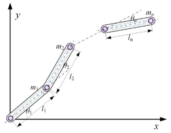
Figure 1. The model of n-link robotic manipulator.

Property 1 [30,31]. $M_r\left(\theta \right)-2C_r\left(\theta ,\dot{\theta }\right)$ is a skew symmetric matrix, and if the variable is $\xi \in R^n$, it satisfies Equation (2).

$${\xi }^T\left(M_r\left(\theta \right)-2C_r\left(\theta ,\dot{\theta }\right)\right)\xi =0.$$

(2)

Property 2 [32]. $M_r\left(\theta \right)$ is a symmetric positive definite matrix of n × n and bounded; if ${\psi }_1$ and ${\psi }_2$ are positive numbers, it satisfies Equation (3).

$${{{\psi }_1‖x‖}^2\le x}^T{M}_r\left(\theta \right)x\ge {\psi }_2{‖x‖}^2 \forall x\in R^n.$$

(3)

Compared with the actual model, the established dynamic system model based on the theoretical structure of the robotic manipulator will have errors in the calculation process. Therefore, the actual dynamic model is established in Equation (4).

$$M_{r0}\left(\theta \right)\ddot{\theta }+C_{r0}\left(\theta ,\dot{\theta }\right)\dot{\theta }+G_{r0}\left(\theta \right)=\tau +f_r\left(\theta ,\dot{\theta },t\right),$$

(4)

where $M_{r0}\left(\theta \right)$, $C_{r0}\left(\theta ,\dot{\theta }\right),$ and $G_{r0}\left(\theta \right)$ are the nominal values of $M_r\left(\theta \right)$, $C_r\left(\theta ,\dot{\theta }\right),$ and $G_r\left(\theta \right)$, respectively. $f_r\left(\theta ,\dot{\theta },t\right)=-∆M_r\left(\theta \right)-∆C_r\left(\theta ,\dot{\theta }\right)-∆G_r\left(\theta \right)-d\left(t\right)$ is the uncertain part of the model, where ${∆M}_r\left(\theta \right)=M_r\left(\theta \right)-M_{r0}\left(\theta \right)$, ${∆C}_r\left(\theta ,\dot{\theta }\right)=C_r\left(\theta ,\dot{\theta }\right)-C_{r0}\left(\theta ,\dot{\theta }\right)$, and ${∆G}_r\left(\theta \right)={G_r\left(\theta \right)-G}_{r0}\left(\theta \right)$, are assumed to have upper bounds. However, in some practical engineering problems, it is easy to choose a larger estimated value for the upper bound. As a result, the control gain is large, which affects the control accuracy and performance. Therefore, it may be a better solution to study model-free control methods that do not require prior knowledge of the upper bound.

2.2. Sliding Mode Control

Under the feedback of the discontinuous state control law function, the control output of an SMC can be continuously switched between two smooth states, which has the characteristics of not requiring an accurate model and being insensitive to parameter changes [33,34]. In this paper, according to the control model’s state feedback error, the function of the sliding surface is used, as shown in Equation (5) [33,35]. The robot’s ideal target trajectory vectors are ${\theta }_d$ and ${\dot{\theta }}_d$. The robot’s actual output trajectory vectors are $\theta$ and $\dot{\theta }$. The angular tracking error is $e={\left[e_1,e_2,\cdots ,e_n\right]}^T$, and the angular velocity tracking error is $\dot{e}={\left[{\dot{e}}_1,{\dot{e}}_2,\cdots ,{\dot{e}}_n\right]}^T$.

$$Sr=\dot{e}+\mathit{\Lambda }e,$$

(5)

where $\mathit{\Lambda }={\mathit{\Lambda }}^T>0$.

According to Equations (1) and (5), the dynamic model error expression is shown in Equation (6).

$$M_r\left(\theta \right)\dot{Sr}=f\left(\theta \right)-C_r\left(\theta ,\dot{\theta }\right)Sr+d\left(t\right)-\tau ,$$

(6)

where $f\left(\theta \right)=M_r\left(\theta \right)\left({\ddot{\theta }}_d+\mathit{\Lambda }\dot{e}\right)+C_r\left(\theta ,\dot{\theta }\right)\left({\dot{\theta }}_d+\mathit{\Lambda }e\right)+G_r\left(\theta \right)$ is the model’s basic information, which is a nonlinear function about $\theta$, $\dot{\theta }$, ${\theta }_d$, ${\dot{\theta }}_d$, and ${\ddot{\theta }}_d$.

The design control rate is shown in Equation (7).

$$\tau =\overline{f}\left(\theta \right)+K_{e}Sr,$$

(7)

where $\overline{f}\left(\theta \right)$ is the theoretical nominal value of $f\left(\theta \right)$ for nominal model control. Equation (8) is obtained by substituting Equation (7) into Equation (6).

$$M_r\left(\theta \right)\dot{Sr}=-\left(K_e+C_r\right)Sr+\tilde{f}\left(\theta \right)+d\left(t\right),$$

(8)

where $\tilde{f}\left(\theta \right)=f\left(\theta \right)-\overline{f}\left(\theta \right)$. The Lyapunov function [36] is defined as $V=\frac{1}{2}{Sr}^T{M}_r\left(\theta \right)Sr$, and its derivative is shown in Equation (9).

$$\dot{V}={Sr}^T{M}_r\dot{Sr}+\frac{1}{2}{Sr}^T\dot{M_r}Sr.$$

(9)

Equation (10) is obtained by substituting Equation (8) into Equation (9).

$$\dot{V}=-{Sr}^T{K}_{e}Sr+\frac{1}{2}{Sr}^T\left(\dot{M_r}-2C_r\right)Sr+{Sr}^T\eta ,$$

(10)

where $\eta =\tilde{f}\left(\theta \right)+d\left(t\right)$.

According to the dynamic model’s oblique symmetry properties, ${Sr}^T\left(\dot{M_r}-2C_r\right)Sr=0$ and $\dot{V}={Sr}^T\eta -{Sr}^T{K}_{e}Sr$ are obtained. The estimation error and disturbance of model information affect the control accuracy and stability. Therefore, in the absence of an accurate dynamic model and accurate judgment of disturbance, researching model approximation and disturbance compensation algorithms is an effective way to achieve high-performance model-free control.

3. Design of PCR-SMC Controller

3.1. Overall Design

A new PCR-SMC controller is proposed in this paper, and its principle is shown in Figure 2. This controller uses a CNN and an RBFNN to parallel trajectory information of different dimensions, so that it can compensate for the robot uncertainty model online and improve the control performance of robot trajectory tracking.

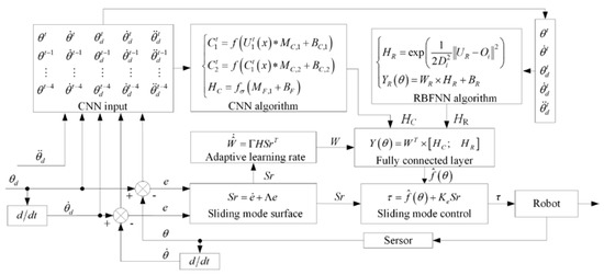
Figure 2. Schematic of the PCR-SMC controller.

In Figure 2, the errors $e$ and $\dot{e}$ are the inputs, and the control torque τ of each joint is the output of the PCR-SMC controller. The input of an RBFNN is composed of five kinds of trajectory information, which are the expected angle ${\theta }_d$, expected angular velocity ${\dot{\theta }}_d$, expected angular acceleration ${\ddot{\theta }}_d$, actual angle $\theta$, and actual angular velocity $\dot{\theta }$. The input of the CNN is the information of the trajectory being retraced. $\widehat{f}\left(\theta \right)$ is the calculation result of the dynamic model identified online by the PCR network, and it participates in trajectory tracking sliding mode control.

3.2. Design of PCR Network

A CNN has the advantages of convolution calculation, local perception, and weight sharing, and it can quickly extract features during data processing. Therefore, its application scenarios gradually penetrate into the field of intelligent industry, which requires a rapid response [37,38]. An RBFNN has the advantages of fast convergence speed, strong robustness, simple structure, and good approximation ability, and it is often used in the field of real-time control [39].

The PCR network structure is designed as shown in Figure 3. In the PCR network, the parallel calculation of an RBFNN and a CNN is performed, and then the calculation results are recomposed into a new network hidden layer; finally, the results are calculated through the output layer. The establishment of the network model and the design of the weight learning algorithm are described in detail below.

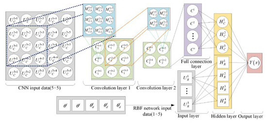
Figure 3. Structure of PCR network.

3.2.1. Convolutional Neural Network

Trajectory information constantly generates changes during the joint motion. Including ${\theta }_d$, ${\dot{\theta }}_d$, ${\ddot{\theta }}_d$, $\theta$, and $\dot{\theta }$, this information affects the system approach and control stability. Therefore, the two-dimensional data of four backtracking moments are selected as the CNN input matrix, with a size of 5 × 5, as shown in Equation (11).

$$U_C=\left[\begin{array}{cc}\begin{array}{cc}\begin{array}{c}\begin{array}{l}{\theta }^t\\ {\theta }^{t-1}\end{array}\\ ⋮\\ {\theta }^{t-4}\hfill \end{array}& \begin{array}{c}\begin{array}{c}{\dot{\theta }}^t\\ {\dot{\theta }}^{t-1}\end{array}\\ ⋮\\ {\dot{\theta }}^{t-4}\end{array}\end{array}& \begin{array}{cc}\begin{array}{c}\begin{array}{c}{\theta }_d^t\\ {\theta }_d^{t-1}\end{array}\\ ⋮\\ {\theta }_d^{t-4}\end{array}& \begin{array}{c}\begin{array}{cc}\begin{array}{c}{\dot{\theta }}_d^t\\ {\dot{\theta }}_d^{t-1}\end{array}& \begin{array}{c}{\ddot{\theta }}_d^t\\ {\ddot{\theta }}_d^{t-1}\end{array}\end{array}\\ \begin{array}{cc}\hfill ⋮\hspace{1em}\hfill & \hfill ⋮\hfill \end{array}\\ \begin{array}{cc}{\dot{\theta }}_d^{t-4}& {\ddot{\theta }}_d^{t-4}\end{array}\end{array}\end{array}\end{array}\right].$$

(11)

The calculation model of the convolutional layer is shown in Equation (12).

$$C_i^t=f_{\sigma }\left({\sigma }_C^t\right)=f\left(U_C^t\left(x\right)\mathrm{*}{M}_{C,i}+B_C\right),i=\mathrm{1,2},\cdots ,M_{C,num},$$

(12)

where $M_C$ represents the convolution kernel, and $M_{C,num}$ represents the number of $M_C$. $B_C$ is the bias, $f_{\sigma }$ is the ReLU function, and its partial derivatives are shown in Equations (13) and (14).

$$f_{\sigma }\left({\sigma }_C\right)=max\left(0,{\sigma }_C\right).$$

(13)

$$\dot{f_{\sigma }}\left({\sigma }_c\right)=\left\{\begin{array}{cc}0& {\sigma }_C\le 0\\ 1& {\sigma }_C>0\end{array}.\right.$$

(14)

The output $H_C$ of the fully connected layer is shown in Equation (15).

$$H_{C,i}=f_{\sigma }\left({\sigma }_F\right)=f_{\sigma }\left(M_{F,i}{C}_i+B_F\right),$$

(15)

where $M_F$ represents the weight of the full connection layer, $B_F$ represents the bias, and $f_{\sigma }$ selects the sigmoid function.

3.2.2. RBF Neural Network

In the PCR network, the dynamic variables $U_R=\left[{\theta }^{t-1},{\dot{\theta }}^{t-1},{\theta }_d^{t-1},{\dot{\theta }}_d^{t-1},{\ddot{\theta }}_d^{t-1}\right]$ of the dynamic model are selected as the input vector of the RBFNN. The nonlinear approximation of the model is realized through a Gaussian hidden layer and output layer [40,41]. The output result $H_R$ of the Gaussian hidden layer is shown in Equation (16).

$$H_{R,i}=exp\left(-\frac{{‖U_R-O_i‖}^2}{2D_i^2}\right),$$

(16)

where $O_i$ is the center point vector, and $D_i$ is the width of the Gaussian.

The hidden layer vector $H$ of the PCR network consists of two kinds of information, which are the result $H_C$ of the CNN and the result $H_R$ of the RBFNN. The output of the PCR network is shown in Equation (17).

$$Y\left(x\right)=W^T\times H,$$

(17)

where $H=\left[H_C;H_R\right]$, and ${W=\left[W_1,W_2,\dots ,W_m\right]}^T$ is the weight of the PCR network output layer.

3.2.3. Weight Update of PCR Network

Gradient descent is a commonly used weight update algorithm in a neural network. The mean square error $E=1/2{\left(Y_d-Y\right)}^2$ is used as the loss function. The weight gradient is defined as the partial derivative of the loss function, as shown in Equation (18).

$${∆W}_t=\partial E\left(W,Y,H\right)/\partial W=\left(Y_d-Y\right)H_t.$$

(18)

The weight update is shown in Equation (19).

$$W_t=W_{t-1}-\mu {∆W}_t,$$

(19)

where $\mu$ is the learning rate.

The PCR network output is used to compensate for an important parameter of the controller, and the loss function cannot be obtained during the system operation. As a result, conventional methods cannot be used for the weight update. To realize the online learning of weight, the adaptive algorithm and the gradient descent are combined. According to Equation (5) and the Lyapunov stability principle [36], the adaptive learning rate of the output layer of the PCR network is designed as shown in Equation (20).

$$\dot{\widehat{W}}=\mathit{\Gamma }HS{r}^T,$$

(20)

where $\mathit{\Gamma }={\mathit{\Gamma }}^T>0$ is the fixed coefficient, and $Sr$ is the sliding mode surface output.

According to the combined features of the PCR network’s hidden layer and the adaptive learning rate, the initial weight update gradient of the CNN can be obtained as $∆W_C={\dot{\hat{W}}}_C-W_C$. Then, the gradient values of each layer in the CNN are calculated by gradient backpropagation. The gradient calculation model of the fully connected layer is shown in Equation (21).

$$∆M_F=H_C\left(1-H_C\right){\left(W_C\right)}^T∆W_C.$$

(21)

According to the weight gradient calculated using the above formula, the fully connected layer weight can be updated as shown in Equation (22).

$$M_F=M_F-\mu \times ∆M_F.$$

(22)

In the PCR network structure, the input vector of the fully connected layer is obtained by reducing the dimension of the last convolutional layer. Therefore, the learning gradient $∆M_{C,2}$ model of the convolution kernel is shown in Equation (23).

$$∆M_{C,2}=\dot{f_{\sigma }}\left({\sigma }_F\right){\left(M_F\right)}^T∆M_F,$$

(23)

where $\dot{f_{\sigma }}\left({\sigma }_F\right)=C_2\left(1-C_2\right)$ is the partial derivative of the sigmoid function, and $C_2$ is the input data of the second convolution layer; the vector form of $∆M_F$ needs to be converted to matrix form. According to the convolution kernel weight gradient $∆M_{C,2}$, a new convolution kernel can be calculated as shown in Equation (24).

$$M_{C,2}=C_2\times ∆M_{C,2}.$$

(24)

The weight gradient $∆M_{C,1}$ of the previous convolution kernel can be calculated through the gradient backpropagation algorithm, as shown in Equation (25).

$$∆M_{C,1}=∆M_{C,2}\times rot180\left(M_{C,2}\right)\times \dot{f_{\sigma }}\left({\sigma }_C\right),$$

(25)

where $rot180\left(M_{C,2}\right)$ means that the matrix $M_{C,2}$ is flipped 180°. $\dot{f_{\sigma }}\left({\sigma }_C\right)$ is the derivative of the ReLU function in the convolutional layer. Given the convolution kernel weight gradient $∆M_{C,1}$, the convolution kernel $M_{C,1}$ can be updated, as shown in Equation (26).

$$M_{C,1}=U_C\left(x\right)\times ∆M_{C,1}$$

(26)

The weight of the PCR network is combined with the adaptive technology and the gradient descent algorithm to realize the online update of the network weight.

3.3. Controller Design

In practical engineering applications, accurate robot dynamic models do not exist, and nominal models are often used for robot trajectory tracking control. However, different nominal models may affect the transformation laws of system errors and degrade control performance. Therefore, the PCR network is used for the online approximation of the dynamic model and compensation for external disturbances, thus achieving model-free control.

The control rate of the PCR-SMC controller is designed as shown in Equation (27).

$$\tau =\widehat{f}\left(\theta \right)+K_{e}Sr,$$

(27)

where $f\left(\theta \right)$ is composed of the robot dynamics model ($M_r{\ddot{q}}_r+C_r{\dot{q}}_r+G_r+f_r$) and external disturbance $d\left(t\right)$; $\widehat{f}\left(\theta \right)$ is the online approximation of $f\left(\theta \right)$ by the PCR network.

Submitting the control rate (Equation (27)) of the controller and the adaptive rate (Equation (20)) of the neural network into Equation (8) yields

$$M_r\dot{Sr}=-\left(C_r+K_e\right)Sr+{\tilde{W}}^{T}H,$$

(28)

and we have

$$M_r\dot{Sr}=-\left(C_r+K_e\right)Sr+{\zeta }_1,$$

(29)

where ${\zeta }_1={\tilde{W}}^{T}H$, $\tilde{W}=W-\widehat{W}$.

Proof. 

The Lyapunov function is shown in Equation (30) [36].

$$L=\frac{1}{2}{Sr}^T{M}_{r}Sr+\frac{1}{2}tr\left({\tilde{W}}^T{F}^{-1}\tilde{W}\right),$$

(30)

where $F=F^T>0$ is the fixed coefficient. □

Deriving Equation (30), we can obtain Equation (31).

$$\dot{L}={Sr}^T{M}_r\dot{Sr}+\frac{1}{2}{Sr}^T\dot{M_r}Sr+tr\left({\tilde{W}}^T{F}^{-1}\dot{\tilde{W}}\right).$$

(31)

Submitting the control rate (Equation (27)) and the neural network’s adaptive rate (Equation (20)) into Equation (31) yields

$$\dot{L}=-{Sr}^T{K}_{e}Sr+\frac{1}{2}{Sr}^T\left(\dot{M_r}-2C_r\right)Sr+tr{\tilde{W}}^T\left(F^{-1}\dot{\tilde{W}}+H{Sr}^T\right).$$

(32)

According to the oblique symmetry characteristic (Equation (2)) of the robot dynamics model, Equation (32) becomes

$$\dot{L}=-{Sr}^T{K}_{e}Sr+tr{\tilde{W}}^T\left(F^{-1}\dot{\tilde{W}}+H{Sr}^T\right),$$

(33)

where $\tilde{W}=W-\widehat{W}$; the ideal weight W is a constant, an $\dot{\tilde{W}}=0-\dot{\widehat{W}}=-\mathit{\Gamma }H{Sr}^T$. According to the operational property of the trace of the matrix ${Sr}^T{\tilde{W}}^{T}H=tr\left({\tilde{W}}^{T}H{Sr}^T\right)$, which transforms Equation (33), we can obtain

$$\dot{L}=-{Sr}^T{K}_{e}Sr.$$

(34)

According to Equation (34), the Lyapunov function is $L\ge 0$, and its derivative is $\dot{L}\le 0$. According to the LaSalle invariance principle, when $t\to 0$, $r\to 0$, $e\to 0$ and $\dot{e}\to 0$. This shows that the control system is asymptotically stable.

4. Numerical Simulation

4.1. Simulation Model and Parameter Setting

This paper organizes numerical simulations for the PCR-SMC controller in the trajectory tracking task of a two-link robot, and the robot is widely used to verify the control algorithm’s performance [42]. The theoretical model of robot dynamics is shown in Equation (35).

$$M_r\left(\theta \right)\ddot{\theta }+C_r\left(\theta ,\dot{\theta }\right)\dot{\theta }+G_r\left(\theta \right)+d\left(t\right)=\tau \left(t\right),$$

(35)

where $\theta ={\left[\begin{array}{cc}{\theta }_1& {\theta }_2\end{array}\right]}^T$, $\tau ={\left[\begin{array}{cc}{\tau }_1& {\tau }_2\end{array}\right]}^T$, and the inertia matrix is $M_r;$ the centrifugal force, Coriolis force matrix $C_r\left(\theta ,\dot{\theta }\right)$, and gravity matrix $G_r\left(\theta \right)$ are shown in Equations (36)–(38), respectively, where $m_i$ is the mass of link i ($m_1=0.5\mathrm{k}\mathrm{g}$, and $m_2=1.5\mathrm{k}\mathrm{g}$), and $l_i$ is the length of link i ($l_1=1\mathrm{m}$ and $l_2=0.8\mathrm{m})$ [43,44]. ${\theta }_i$ and ${\dot{\theta }}_i$ represent the angle and angular velocity of link i, respectively; g = 9.81 m/s².

$$M_r\left(\theta \right)=\left[\begin{array}{cc}{Z}_1+Z_2+2Z_3\cos {\theta }_2& Z_2+Z_3\cos {\theta }_2\\ m_2{l}_2^2+m_2{l}_1{l}_2\cos {\theta }_2& m_2{l}_2^2\end{array}\right],$$

(36)

$$C_r\left(\theta ,\dot{\theta }\right)=\left[\begin{array}{cc}{-Z_3\dot{\theta }}_2\mathit{sin}{\theta }_2& -Z_3\left({\dot{\theta }}_1+{\dot{\theta }}_2\right)\mathit{sin}{\theta }_2\\ Z_3{\dot{\theta }}_1\mathit{sin}{\theta }_2& 0\end{array}\right],$$

(37)

$$G_r\left(\theta \right)=\left[\begin{array}{c}{Z}_4\mathit{cos}\left({{\theta }_1+\theta }_2\right)+Z_5\mathit{cos}{\theta }_1\\ Z_4\mathit{cos}\left({{\theta }_1+\theta }_2\right)\end{array}\right],$$

(38)

where $Z_1=\left(m_1+m_2\right)l_1^2$, $Z_2=m_2{l}_2^2$, $Z_3=m_2{l}_1{l}_2$, $Z_4=m_2{l}_2\mathrm{g}$, and $Z_5=\left(m_1+m_2\right)l_1\mathrm{g}$.

The parameters of SMC are set as follows: $K_e=[\mathrm{24,0};\mathrm{0,24}]$, $\mathit{\Lambda }=[\mathrm{13,0};\mathrm{0,13}]$, and $\mathit{\Gamma }=[\mathrm{20,0};\mathrm{0,20}]$. Table 1 gives the parameters of the PCR network structure. The input of RBFNN is $U_R=\left[{\theta }^{t-1},{\dot{\theta }}^{t-1},{\theta }_d^{t-1},{\dot{\theta }}_d^{t-1},{\ddot{\theta }}_d^{t-1}\right]$. The input data of CNN are composed of the two-dimensional information of joint trajectories in the past five iterations, as shown in Equation (11). In addition, the RBF-SMC controller is a contrast control algorithm, and its network structure is 5–7–1. The parameters of the RBFNN part of the PCR-SMC and RBF-SMC controllers are set identically.

Table 1. Parameters of PCR network.

Parameters	Value
Number of convolution kernels ($M_{C,num}$)	2
Size ${(M}_{C,1})$	2 × 2
Size $\left(M_{C,2}\right)$	3 × 3
Learning rate ($\mu$)	0.005
Number of hidden layers ($H$)	7

4.2. Simulation Results and Analysis

Case 1. The control performance of the PCR-SMC controller is verified in a normal trajectory and compared with the RBF-SMC controller. The desired trajectory is shown in Equation (39) [45].

$${\theta }_d\left(t\right)=\left[\begin{array}{c}1.25-\left(7/5\right)e^{-t}+\left(7/20\right)e^{-4t}\\ 1.25+e^{-t}-\left(1/4\right)e^{-4t}\end{array}\right].$$

(39)

The initial values of the joint angle are ${\theta }_1\left(0\right)=0.3$ and ${\theta }_2\left(0\right)=1.9$, and the angular velocity is 0. During the 20 s simulation, random disturbance is added, and the amplitude is set to 0.1, which is used to simulate the external disturbance in the actual working condition. In addition, to effectively judge the response speed, convergence ability, and stability of the control algorithm, the externally changing load disturbance is added during the simulation for 5–10 s, as shown in Equation (40) [46]. After 15 s, the fixed load disturbance is added as [−15; −10] [47].

$$\left[\begin{array}{c}-2.14\mathit{cos}\left(10t\right)+2\\ 4.15\mathit{sin}\left(20t-\pi /4\right)\end{array}\right].$$

(40)

Figure 4, Figure 5, Figure 6 and Figure 7 show the trajectory tracking simulation results and absolute errors. The estimated performance of the PCR network is shown in Figure 8, and the output control torque is shown in Figure 9. Both the PCR-SMC and RBF-SMC controllers have obvious convergence trends before applying the load. However, the tracking error of the RBF-SMC controller is larger than that of the PCR-SMC controller. After 5 s, a continuously varying load is applied. The tracking error of the RBF-SMC controller has a large oscillation, while the PCR-SMC controller has strong anti-interference ability, and the control error is in a small interval. After 15 s, the fixed load is applied, and the control torque and network output gradually converge to a new value. The control output and trajectory tracking process of the PCR-SMC controller are more stable. This shows that the PCR-SMC controller has strong control stability and superior control performance to the RBF-SMC controller.

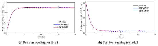
Figure 4. Desired and actual tracked trajectories of links on a normal trajectory.

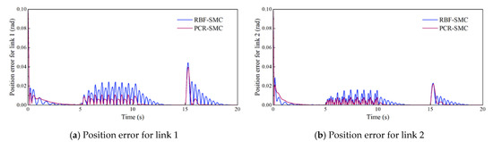
Figure 5. Trajectory tracking absolute error on a normal trajectory.

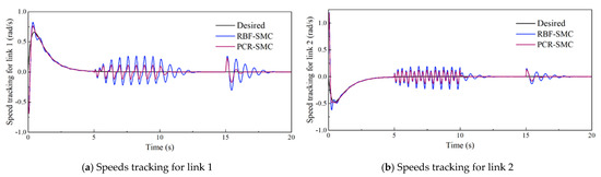
Figure 6. Desired and actual tracking speeds of links on a normal trajectory.

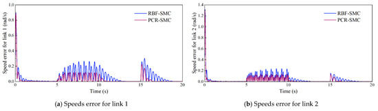
Figure 7. Speed tracking absolute error on a normal trajectory.

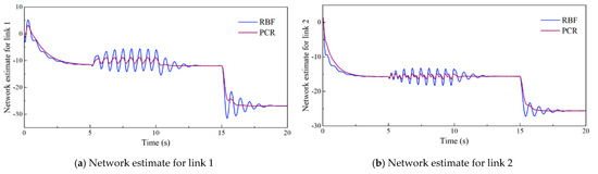
Figure 8. Network estimation output on a normal trajectory.

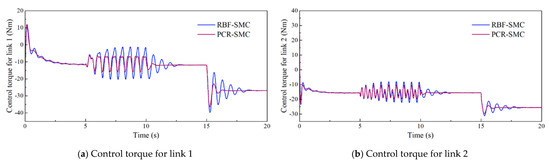
Figure 9. Control torque on a normal trajectory.

Table 2, Table 3 and Table 4 show the mean absolute error (MAE) and standard deviation (SD) of the tracking results, including the overall control process (0–20 s), the control of variable disturbances (5–10 s), and the control of fixed disturbances (15–20 s). The MAE evaluates the tracking accuracy, and the SD evaluates the tracking stability of the trajectory. By analyzing the simulation results in the tables, we determined that the PCR-SMC controller reduces the trajectory tracking error and improves stability compared with the RBF-SMC method.

Table 2. Overall tracking error (0–20 s).

Error		PCR-SMC		RBF-SMC
		Link 1	Link 2	Link 1	Link 2
Position error	MAE	0.0039	0.0031	0.0066	0.0041
	SD	0.0135	0.0130	0.0153	0.0134
Speed error	MAE	0.0215	0.0241	0.0501	0.0366
	SD	0.0366	0.0941	0.1014	0.1050

Table 3. Tracking error with variable disturbance (5–10 s).

Error		PCR-SMC		RBF-SMC
		Link 1	Link 2	Link 1	Link 2
Position error	MAE	0.0054	0.0037	0.0117	0.0064
	SD	0.0061	0.0043	0.0135	0.0078
Speed error	MAE	0.0517	0.0663	0.1131	0.0969
	SD	0.0661	0.1361	0.0761	0.1157

Table 4. Tracking error with fixed interference (15–20 s).

Error		PCR-SMC		RBF-SMC
		Link 1	Link 2	Link 1	Link 2
Position error	MAE	0.0018	0.0012	0.0050	0.0023
	SD	0.0064	0.0038	0.0094	0.0046
Speed error	MAE	0.0109	0.0065	0.0420	0.0184
	SD	0.0369	0.0741	0.0202	0.0337

Case 2. The starfish-shaped trajectory is a more complex robot trajectory, which can further verify the effectiveness and stability of the PCR-SMC controller. The starfish-shaped trajectory model is shown in Equation (41).

$$\left[\begin{array}{c}\left(0.8+0.2\times sin\left(5t\right)\right)\times cos\left(t+4\pi /3\right)\\ \left(0.8+0.2\times sin\left(5t\right)\right)\times sin\left(t+4\pi /3\right)\end{array}\right].$$

(41)

The initial values of $\theta$ and $\dot{\theta }$ are set to 0, and the others are the same as those in Case 1. The tracking results of the starfish trajectory at the robot’s end-effector are shown in Figure 10. Figure 11 and Figure 12 show the trajectory tracking results of the links. The model uncertainty approximation results based on the neural network are shown in Figure 13. The PCR-SMC controller has high tracking accuracy, and the output of the PCR network is more stable, showing better control performance. The effectiveness and versatility of the PCR-SMC controller are fully verified.

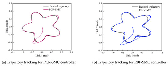
Figure 10. Robot end-effector trajectory tracking results.

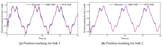
Figure 11. Desired and actual tracked trajectories of links on a starfish-shaped trajectory.

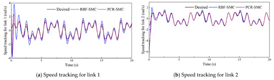
Figure 12. Desired and actual tracking speeds of links on a starfish-shaped trajectory.

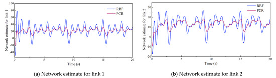
Figure 13. Network estimation output on a starfish-shaped trajectory.

From the simulation results of the above two trajectory tracking control methods (see Figure 8 and Figure 13), we determined that, in the online approximation process of system model uncertainty, the output of the PCR network can converge rapidly, and the process is more stable, compared with the RBFNN. This shows that the feature value extracted by the CNN in the historical trajectory data is an important parameter for system model identification. Historical feature information is reasonably used, and it can effectively improve the identification accuracy and control stability of the dynamic model, improving the system’s control performance.

The simulation results of the PCR-SMC controller proposed in this study were compared with other controllers, and the comparison results are shown in Table 5. In the case of varying load and fixed load interference, the proposed PCR-SMC controller achieved excellent control results and demonstrated excellent competitiveness.

Table 5. Controller comparison results.

Controller	Robot Type	Maximum Error	MAE	External Interference
PCR-SMC controller	2DOF	0.1 rad	0.0039 rad	Varying and fixed load
Adaptive controller [28]	2DOF	Near 0.2 rad	-	No
RFISMSC [35]	2DOF	0.1 rad	-	No
AISMC-TDE [45]	2DOF	Near 0.43 rad	0.0149 rad	Varying load
Adaptive controller [47]	2DOF	Near 0.4 rad	-	Fixed load
Robust control system [48]	2DOF	0.28 rad	-	No
HOSMC [49]	2DOF	Near 0.7 rad	-	Lower load

5. Conclusions

This paper proposed a new PCR-SMC controller and applied it to the trajectory tracking control problem of a two-link robot. We considered factors affecting trajectory tracking accuracy, including mechanical model uncertainties and external disturbances. The effective approximation and compensation of the model was realized by constructing a PCR network. Meanwhile, a new online learning algorithm was designed, by integrating adaptive control and the gradient descent method. The online learning mechanism can effectively adjust the connection weight of PCR network in real time, and the stability of the control system was proven by Lyapunov’s theory. The simulation was performed with normal and starfish-shaped trajectories. The results showed that the PCR-SMC controller effectively reduced the trajectory tracking errors on both trajectories, compared with the RBF-SMC controller. This shows that the PCR-SMC controller has higher tracking accuracy, strong stability to model uncertainty and external disturbance, and excellent control performance.

In future work, we will further improve the control performance of the sliding mode controller based on the PCR network by compensating for the uncertainty of the dynamic model, and enriching the controller’s application field.

References

- Yu, X.; He, W.; Li, H.; Sun, J. Adaptive fuzzy full-state and output-feedback control for uncertain robots with output constraint. IEEE Trans. Syst. Man Cybern. Syst. 2020, 51, 6994–7007. [Google Scholar] [CrossRef]
- Ghafarian, M.; Shirinzadeh, B.; Al-Jodah, A.; Das, T.K. Adaptive fuzzy sliding mode control for high-precision motion tracking of a multi-DOF micro/nano manipulator. IEEE Robot. Autom. Lett. 2020, 5, 4313–4320. [Google Scholar] [CrossRef]
- Sharma, R.; Kumar, V.; Gaur, P.; Mittal, A.P. An adaptive PID like controller using mix locally recurrent neural network for robotic manipulator with variable payload. ISA Trans. 2016, 62, 258–267. [Google Scholar] [CrossRef] [PubMed]
- Malik, A.A.; Masood, T.; Bilberg, A. Virtual reality in manufacturing: Immersive and collaborative artificial-reality in design of human-robot workspace. Int. J. Comput. Integr. Manuf. 2020, 33, 22–37. [Google Scholar] [CrossRef]
- Wei, B. Adaptive control design and stability analysis of robotic manipulators. Actuators 2018, 7, 89. [Google Scholar] [CrossRef]
- Tang, F.; Niu, B.; Wang, H.; Zhang, L.; Zhao, X. Adaptive fuzzy tracking control of switched MIMO nonlinear systems with full state constraints and unknown control directions. IEEE Trans. Circuits Syst. II Express Briefs 2022, 69, 2912–2916. [Google Scholar] [CrossRef]
- Galvan-Perez, D.; Yañez-Badillo, H.; Beltran-Carbajal, F.; Rivas-Cambero, I.; Favela-Contreras, A.; Tapia-Olvera, R. Neural Adaptive Robust Motion-Tracking Control for Robotic Manipulator Systems. Actuators 2022, 11, 255. [Google Scholar] [CrossRef]
- Chen, L.; Yan, B.; Wang, H.; Shao, K.; Kurniawan, E.; Wang, G. Extreme-learning-machine-based robust integral terminal sliding mode control of bicycle robot. Control. Eng. Pract. 2022, 121, 105064. [Google Scholar] [CrossRef]
- Hu, H.; Bei, S.; Zhao, Q.; Han, X.; Zhou, D.; Zhou, X.; Li, B. Research on Trajectory Tracking of Sliding Mode Control Based on Adaptive Preview Time. Actuators 2022, 11, 34. [Google Scholar] [CrossRef]
- Xu, C.Z. Research on Intelligent Backstepping Sliding Mode Control of Nonlinear Robots. Doctoral Dissertation, Huaqiao University, Quanzhou, China, 2012. [Google Scholar]
- Zhao, T.; Liu, J.; Dian, S.; Guo, R.; Li, S. Sliding-mode-control-theory-based adaptive general type-2 fuzzy neural network control for power-line inspection robots. Neurocomputing 2020, 401, 281–294. [Google Scholar] [CrossRef]
- Yang, Z.Y.; Wu, J.; Mei, J.P. Motor-mechanism dynamic model based neural network optimized computed torque control of a high speed parallel manipulator. Mechatronics 2007, 17, 381–390. [Google Scholar] [CrossRef]
- Gao, H.; Xiong, L. Research on a hybrid controller combining RBF neural network supervisory control and expert PID in motor load system control. Adv. Mech. Eng. 2022, 14, 16878132221109994. [Google Scholar] [CrossRef]
- Cheng, X.; Liu, H.; Lu, W. Chattering-suppressed sliding mode control for flexible-joint robot manipulators. Actuators 2021, 10, 288. [Google Scholar] [CrossRef]
- Yin, F.C.; Ji, Q.Z.; Wen, C.W. An adaptive terminal sliding mode control of stone-carving robotic manipulators based on radial basis function neural network. Appl. Intell. 2022, 52, 1–18. [Google Scholar] [CrossRef]
- Fang, W.; Chao, F.; Lin, C.M.; Zhou, D.; Yang, L.; Chang, X.; Shen, Q.; Shang, C. Visual-guided robotic object grasping using dual neural network controllers. IEEE Trans. Ind. Inform. 2020, 17, 2282–2291. [Google Scholar] [CrossRef]
- Chen, D.; Zhang, J.; Li, Z. A novel fixed-time trajectory tracking strategy of unmanned surface vessel based on the fractional sliding mode control method. Electronics 2022, 11, 726. [Google Scholar] [CrossRef]
- Ye, T.; Luo, Z.; Wang, G. Adaptive sliding mode control of robot based on fuzzy neural network. J. Ambient. Intell. Humaniz. Comput. 2020, 11, 6235–6247. [Google Scholar] [CrossRef]
- Yen, V.T.; Nan, W.Y.; Van Cuong, P. Robust adaptive sliding mode neural networks control for industrial robot manipulators. Int. J. Control. Autom. Syst. 2019, 17, 783–792. [Google Scholar] [CrossRef]
- Wang, D.H.; Zhang, S.J. Improved neural network-based adaptive tracking control for manipulators with uncertain dynamics. Int. J. Adv. Robot. Syst. 2020, 17, 1729881420947562. [Google Scholar] [CrossRef]
- Zhang, C.; Huang, Q.; Zhang, C.; Yang, K.; Cheng, L.; Li, Z. ECNN: Intelligent Fault Diagnosis Method Using Efficient Convolutional Neural Network. Actuators 2022, 11, 275. [Google Scholar] [CrossRef]
- Yao, X.; Chen, Z. Sliding mode control with deep learning method for rotor trajectory control of active magnetic bearing system. Trans. Inst. Meas. Control. 2019, 41, 1383–1394. [Google Scholar] [CrossRef]
- Zhou, M.; Feng, Y.; Xue, C.; Han, F. Deep convolutional neural network based fractional-order terminal sliding-mode control for robotic manipulators. Neurocomputing 2020, 416, 143–151. [Google Scholar] [CrossRef]
- Hemalakshmi, G.R.; Santhi, D.; Mani, V.R.S.; Geetha, A.; Prakash, N.B. Classification of retinal fundus image using MS-DRLBP features and CNN-RBF classifier. J. Ambient. Intell. Humaniz. Comput. 2021, 12, 8747–8762. [Google Scholar] [CrossRef]
- Hong, Y.Y.; Rioflorido, C.L.P.P. A hybrid deep learning-based neural network for 24-h ahead wind power forecasting. Appl. Energy 2019, 250, 530–539. [Google Scholar] [CrossRef]
- Sideratos, G.; Ikonomopoulos, A.; Hatziargyriou, N.D. A novel fuzzy-based ensemble model for load forecasting using hybrid deep neural networks. Electr. Power Syst. Res. 2020, 178, 106025. [Google Scholar] [CrossRef]
- Liu, J. Robot Control System Design and Matlab Simulation: Basic Design Method; Press of Tsinghua University: Beijing, China, 2016; pp. 20–35. [Google Scholar]
- Liu, A.; Zhao, H.; Song, T.; Liu, Z.; Wang, H.; Sun, D. Adaptive control of manipulator based on neural network. Neural Comput. Appl. 2021, 33, 4077–4085. [Google Scholar] [CrossRef]
- Lu, P.; Huang, W.; Xiao, J.; Zhou, F.; Hu, W. Adaptive Proportional Integral Robust Control of an Uncertain Robotic Manipulator Based on Deep Deterministic Policy Gradient. Mathematics 2021, 9, 2055. [Google Scholar] [CrossRef]
- Yu, X.; Zhang, S.; Fu, Q.; Xue, C.; Sun, W. Fuzzy Logic Control of an Uncertain Manipulator with Full-State Constraints and Disturbance Observer. IEEE Access 2020, 8, 24284–24295. [Google Scholar] [CrossRef]
- Nohooji, H.R. Constrained neural adaptive PID control for robot manipulators. J. Frankl. Inst. 2020, 357, 3907–3923. [Google Scholar] [CrossRef]
- Özyer, B. Adaptive fast sliding neural control for robot manipulator. Turk. J. Electr. Eng. Comput. Sci. 2020, 28, 3154–3167. [Google Scholar]
- Feng, H.; Song, Q.; Ma, S.; Ma, W.; Yin, C.; Cao, D.; Yu, H. A new adaptive sliding mode controller based on the RBF neural network for an electro-hydraulic servo system. ISA Trans. 2022, 129, 472–484. [Google Scholar] [CrossRef] [PubMed]
- Zhang, F.; Xiao, H.; Zhang, Y.; Gong, G. Distributed Drive Electric Bus Handling Stability Control Based on Lyapunov Theory and Sliding Mode Control. Actuators 2022, 11, 85. [Google Scholar] [CrossRef]
- Zhang, X.; Xu, W.; Lu, W. Fractional-order iterative sliding mode control based on the neural network for manipulator. Math. Probl. Eng. 2021, 2021, 1–12. [Google Scholar] [CrossRef]
- Gao, L.; Xiong, L.; Lin, X.; Xia, X.; Liu, W.; Lu, Y.; Yu, Z. Multi-sensor fusion road friction coefficient estimation during steering with lyapunov method. Sensors 2019, 19, 3816. [Google Scholar] [CrossRef]
- Gabdullin, N.; Madanzadeh, S.; Vilkin, A. Towards end-to-end deep learning performance analysis of electric motors. Actuators 2021, 10, 28. [Google Scholar] [CrossRef]
- Abdou, M.A. Literature review: Efficient deep neural networks techniques for medical image analysis. Neural Comput. Appl. 2022, 34, 5791–5812. [Google Scholar] [CrossRef]
- Ding, S.; Zhao, H.; Zhang, Y.; Xu, X.; Nie, R. Extreme learning machine: Algorithm, theory and applications. Artif. Intell. Rev. 2015, 44, 103–115. [Google Scholar] [CrossRef]
- Van Cuong, P.; Nan, W.Y. Adaptive trajectory tracking neural network control with robust compensator for robot manipulators. Neural Comput. Appl. 2016, 27, 525–536. [Google Scholar] [CrossRef]
- Nadeem, F.; Alghazzawi, D.; Mashat, A.; Fakeeh, K.; Almalaise, A.; Hagras, H. Modeling and predicting execution time of scientific workflows in the grid using radial basis function neural network. Clust. Comput. 2017, 20, 2805–2819. [Google Scholar] [CrossRef]
- Yang, X.; Sun, W.; Dong, H.; Wu, X. Adaptive Prescribed Performance Fuzzy Control for n-Link Flexible-Joint Robots Under Event-Triggered Mechanism. Int. J. Fuzzy Syst. 2022, 25, 1019–1033. [Google Scholar] [CrossRef]
- Feng, Y.; Yu, X.; Man, Z. Non-singular terminal sliding mode control of rigid manipulators. Automatica 2002, 38, 2159–2167. [Google Scholar] [CrossRef]
- Nojavanzadeh, D.; Badamchizadeh, M. Adaptive fractional-order non-singular fast terminal sliding mode control for robot manipulators. IET Control. Theory Appl. 2016, 10, 1565–1572. [Google Scholar] [CrossRef]
- Wang, H.; Fang, L.; Song, T.; Xu, J.; Shen, H. Model-free adaptive sliding mode control with adjustable funnel boundary for robot manipulators with uncertainties. Rev. Sci. Instrum. 2021, 92, 065101. [Google Scholar] [CrossRef] [PubMed]
- Zhang, X.; Shi, R. Adaptive Fractional-Order Nonsingular Fast Terminal Sliding Mode Control for Manipulators. Complexity 2021, 2021, 1–13. [Google Scholar] [CrossRef]
- Liu, Q.; Li, D.; Ge, S.S.; Ji, R.; Ouyang, Z.; Tee, K.P. Adaptive bias RBF neural network control for a robotic manipulator. Neurocomputing 2021, 447, 213–223. [Google Scholar] [CrossRef]
- Chang, Z.; Hao, L.; Yan, Q.; Ye, T. Research on manipulator tracking control algorithm based on RBF neural network. J. Phys. Conf. Ser. 2021, 1802, 032072. [Google Scholar] [CrossRef]
- Lin, C.J.; Sie, T.Y.; Chu, W.L.; Yau, H.T.; Ding, C.H. Tracking control of pneumatic artificial muscle-activated robot arm based on sliding-mode control. Actuators 2021, 10, 66. [Google Scholar] [CrossRef]
Disclaimer/Publisher’s Note: The statements, opinions and data contained in all publications are solely those of the individual author(s) and contributor(s) and not of MDPI and/or the editor(s). MDPI and/or the editor(s) disclaim responsibility for any injury to people or property resulting from any ideas, methods, instructions or products referred to in the content. |
© 2023 by the authors. Licensee MDPI, Basel, Switzerland. This article is an open access article distributed under the terms and conditions of the Creative Commons Attribution (CC BY) license (https://creativecommons.org/licenses/by/4.0/).