Article

A Multi-Scale Attention Mechanism Based Domain Adversarial Neural Network Strategy for Bearing Fault Diagnosis

1
Institute of Intelligent Manufacturing, Nanjing Tech University, Nanjing 210009, China
2
College of Mechanical and Power Engineering, Nanjing Tech University, Nanjing 211816, China
3
College of Electrical Engineering and Control Science, Nanjing Tech University, Nanjing 211816, China
*
Author to whom correspondence should be addressed.
Actuators 2023, 12(5), 188; https://doi.org/10.3390/act12050188
Submission received: 27 March 2023 / Revised: 22 April 2023 / Accepted: 26 April 2023 / Published: 27 April 2023
(This article belongs to the Special Issue Dynamics and Control of Aerospace Systems)

Abstract

:
There are a large number of bearings in aircraft engines that are subjected to extreme operating conditions, such as high temperature, high speed, and heavy load, and their fatigue, wear, and other failure problems seriously affect the reliability of the engine. The complex and variable bearing operating conditions can lead to differences in the distribution of data between the source and target operating conditions, as well as insufficient labels. To solve the above challenges, a multi-scale attention mechanism-based domain adversarial neural network strategy for bearing fault diagnosis (MADANN) is proposed and verified using Case Western Reserve University bearing data and PT500mini mechanical bearing data in this paper. First, a multi-scale feature extractor with an attention mechanism is proposed to extract more discriminative multi-scale features of the input signal. Subsequently, the maximum mean discrepancy (MMD) is introduced to measure the difference between the distribution of the target domain and the source domain. Finally, the fault diagnosis process of the rolling is realized by minimizing the loss of the feature classifier, the loss of the MMD distance, and maximizing the loss of the domain discriminator. The verification results indicate that the proposed strategy has stronger learning ability and better diagnosis performance than shallow network, deep network, and commonly used domain adaptive models.

1. Introduction

Rotating bearing is some of the core components of the most important machinery equipment, such as the aero-engine, the high-speed axle box, etc. Under harsh environments, such as high temperature and high pressure for a long time, the performance of the rolling bearing will inevitably deteriorate, even leading to the failure of the aero-engine, the high-speed axle box, and other equipment [1,2,3]. Furthermore, due to the closed-loop regulation of the system, external environmental interference, especially the change in working conditions, the fault characteristics of the system are easily covered up [4]. If the fault cannot be identified timely and effectively, it will cause great economic losses and even cause great accidents. Therefore, bearing fault diagnosis is very important in aerospace, automobile, and railway industries [5,6].
Driven by this motivation, various fault diagnosis methods have been fully developed in recent years. Especially with the rapid development of signal processing, data mining and artificial intelligence technology, data-driven fault diagnosis methods have been applied to the field of bearing fault diagnosis [7]. Some machine learning based methods have been successfully applied. The machine learning-based bearing fault diagnosis method generally includes signal feature extraction [8] and fault classification. Common feature extraction methods include Fourier transform [9], wavelet transform [10], variational mode decomposition [11], etc. Fault classification methods commonly include artificial neural network [12,13,14] and support vector machine [15,16,17]. Although these fault diagnosis methods can realize automatic fault identification and improve the efficiency of fault diagnosis, these machine learning-based methods have a shallow structure and rely on manual experience. Their diagnosis accuracy is closely related to feature extraction. Facing the above challenges, the deep learning-based diagnosis methods have made great progress because deep learning has stronger feature capture, better big data processing capabilities, and superior performance in multi-layer nonlinear mapping and processing large-scale mechanical data than the shallow network [18]. What is more, the use of a multi-layer structure can eliminate the dependence on human and expert knowledge. Among many deep learning methods, the convolutional neural network (CNN) has been successfully applied in the field of intelligent fault identification due to its weight sharing, local perception, and strong anti-noise ability [19,20,21,22,23,24,25,26,27,28,29].
The above fault diagnosis methods are all based on constant working conditions. However, in practical engineering, operational conditions of the equipment are not constant due to the continuous change in the production environment and working conditions. The neural network-based fault diagnosis method under constant working conditions is not enough to effectively identify all fault types. The changing working conditions will cause vibration signal amplitude changes, pulse interval changes, and other problems. Deep learning models, such as CNN, cannot solve the problem of data distribution difference under variable working conditions because it is expensive to collect a large number of labeled data. Therefore, domain adaptive technology, combined with CNN, is proposed to solve the problem of difficulty to obtain labeled data under current working conditions. For instance, Wang et al. [30] used a domain adversarial neural network (DANN) with a domain discriminator to mine domain invariant features under different devices. Li et al. [31] proposed a migration learning network based on DANN to identify shared fault types in two domains and to learn new fault types. Lu et al. [32] proposed a depth domain adaptive structure. This structure can adapt both the conditional distribution and the edge distribution in the multi-layer neural network and use maximum mean discrepancy (MMD) to measure the distribution difference. Wu et al. [33] proposed a novel intelligent recognition method based on an adversarial domain adaptation convolutional neural network (ADACNN). The ADACNN introduced MMD in the prediction label space for domain adaptation to alleviate the problem of algorithm performance degradation, which is caused by the distribution deviation between the test data and the training data. Wu et al. [34] adopted a cost-sensitive depth classifier to solve the problem of class imbalance, and they used the domain counter subnet with MMD to simultaneously minimize the marginal and conditional distribution differences between the source domain and the target domain. Liu et al. [35] proposed a migration learning fault diagnosis model based on a deep full convolution conditional Wasserstein adversarial network (FCWAN), which uses the conditional countermeasure mechanism to enhance the effect of migration domain adaptation and further improve the accuracy of diagnosis. Zou et al. [36] proposed a deep convolution Wasserstein adversarial network (DCWAN)-based fault transfer diagnosis model. This model solved the problem of inadequate self-adaptive measurement of feature distribution differences under different working conditions, increased variance constraints to improve the aggregation of extracted features, and expanded the margins between different types of features in the source domain. Wu et al. [37] proposed a Gaussian-guided adversarial adaption transfer network (GAATN) for bearing fault diagnosis. GAATN introduced a Gaussian-guided distribution alignment strategy to make the data distribution of two domains close to the Gaussian distribution to reduce data distribution discrepancies.
In summary, most scholars have studied various deep learning methods from different angles to improve their performance in bearing fault diagnosis. However, the importance of the features extracted by the feature extractors is different. The existing domain adaptive methods seldom pay attention to the more discriminative features and use a single scale extraction when extracting features, and the model performance will be poor due to the lack of information. Therefore, a multi-scale attention mechanism domain adversarial neural network for bearing fault diagnosis (MADANN) will be discussed in this article. Specifically, the main contributions are as follows:
(1)
A feature extractor based on a multi-scale convolution structure and attention mechanism is designed. It is adopted to broaden the network width, fuse feature information of different scales, focus on the key features with identification ability to suppress irrelevant features, and improve the accuracy of fault identification.
(2)
A class domain adaptation based on the maximum mean difference is designed. MMD is introduced into the predictive label space for domain adaptation to measure the distribution difference between the target and source domains.
(3)
Experimental results on a public bearing dataset and data collected by the test bench confirm that the proposed methodology has higher recognition accuracy.
The rest of this paper is arranged as follows. Section 1 introduces the relevant theories of domain adversarial network, maximum mean discrepancy, and attention mechanism. Section 2 introduces the proposed rolling bearing fault diagnosis model of domain adversarial migration based on multi-scale and attention mechanism. Section 3 uses two different data sets to verify the effectiveness of the proposed method. Finally, this is all summarized in Section 4.

2. Theoretical Background

2.1. Domain Adversarial Neural Network

The DANN network is composed of three parts: feature extractor G f , label classifier G y , and domain discriminator G d . A gradient reverse layer (GRL) is added between the feature extractor and the domain discriminator.
The structure of DANN is as shown in Figure 1. First, the source domain data X s = { x s i , y s i } n s i = 1 and the target domain data X t = { x t i } n t i = 1 are input to the feature extractor G f to extract the source domain feature G ( x i s , θ f ) and target domain feature G ( x i t , θ f ) , as well as to input the extracted source domain feature G ( x i s , θ f ) to the label classifier for classification. The label L y loss operation is:
L y i ( θ f , θ y ) = L y i ( G y ( G f ( x i s ) ) , y i s ) = P i s log 1 G y ( G f ( x i s ) ) , y i s ) ,
L y ( θ f , θ y ) = 1 n s i = 1 n s L y i ( G y ( G f ( x i s ) ) , y i s ) ,
where P i s represents 0 or 1. If the true category of sample i is equal to s, take 1, otherwise take 0. θ f represents parameters in the feature extraction module. θ y represents parameters in the fault diagnosis classification module. y i is the label of the bearing. G f ( x i s ) is the output of the ith source domain sample mapped by the feature extractor, and n s is the number of samples.
At the same time, input the source domain feature G ( x i s , θ f ) and the target domain feature G ( x i s , θ f ) to the domain discriminator to determine whether the extracted feature is from the target domain or the source domain. Since adding a gradient reversal layer between the domain discriminator and the feature extractor, the gradient of the incoming feature extractor G f during the reverse propagation of L d is λ L d θ f . At this time, G f optimization will increase the error of the domain discriminator, and the parameter θ f is learned by maximizing the loss function L d of the domain discriminator, while the gradient in the domain discriminator G d is L d θ d , and the parameter θ d is learned by minimizing the loss function L d of the domain discriminator. The domain discriminator loss operation L d is:
L d = 1 n s i = 1 n s L d i ( θ f , θ d ) + 1 n t j = 1 n t L d j ( θ f , θ d ) ,
L d i ( θ f , θ d ) = L d ( G d ( G f ( x i ) ) , d i ) = d i log 1 G d ( G f ( x i ) ) + ( 1 d i ) log 1 G d ( G f ( x i ) ) ,
where θ f and θ d , respectively, represent the parameters of the feature extractor and the domain discriminator, n s is the number of samples in the source domain, and n t is the number of samples in the target domain.
The overall objective function is:
L ( θ f , θ y , θ d ) = 1 n s i = 1 n s L y i ( θ f , θ y ) λ ( 1 n s i = 1 n s L d i ( θ f , θ d ) + 1 n t j = 1 n t L d j ( θ f , θ d ) ) ,
The final optimization result is obtained in θ ^ f , θ ^ d , θ ^ y and the expression is:
θ ^ f , θ ^ y = arg min θ f , θ y   L ( θ f , θ y , θ ^ d ) ,
θ ^ d = arg min θ d   L ( θ ^ f , θ ^ y , θ d ) ,

2.2. Maximum Mean Discrepancy

Suppose there are two data sets, source domain data set X s = { x s i , y s i } n s i = 1 with label and target domain data set X t = { x t i } n t i = 1 without label. Where n s represents the number of samples of the source domain data, n t represents the number of samples of the target domain data, and y i s represents the data label of the source domain. These two datasets have the same label space y s = y t and follow different distributions P s ( X ) , P t ( X ) . Therefore, the square of the MMD distance of x s ,   x t can be defined as:
M M D 2 ( X s , X t ) = 1 n s i = 1 n s Φ ( x i s ) 1 n t j = 1 n t Φ ( x j t ) H 2 ,
where Φ ( · ) represents the nonlinear mapping function of the reproducing kernel Hilbert space (RKHS).
To simplify the above functions, the kernel function is introduced in the formula, and the square of MMD distance is rewritten as:
M M D 2 ( X s , X t ) = 1 n s n s i = 1 n s j = 1 n s k ( x i s , x j s ) + 1 n t n t i = 1 n t j = 1 n t k ( x i t , x j t ) 2 n s n t i = 1 n s j = 1 n t k ( x i s , x j t ) ,
where k ( x i s , x j t ) = Φ ( x i s ) , Φ ( x j t ) represents a kernel function.
Select the Gaussian kernel as the kernel function because it can map data to an infinite dimensional space. The formula of the Gaussian kernel function is as follows:
k ( x s , x t ) = e x s x t 2 2 σ 2 ,
where σ is the kernel bandwidth, and, if σ 0 , the MMD will be 0. Similarly, if the larger bandwidth is σ , the MMD will also be 0. To solve this problem, the kernel bandwidth σ is selected as the median distance between all sample pairs, that is:
σ 2 = E x s x t 2 ,
Different kernel functions will be mapped to different regenerated kernel Hilbert spaces to form different distributions. To reduce the influence of Gaussian kernel functions on the results, multiple Gaussian kernels are used to construct multi kernel functions. The definition of multi kernel functions is as follows:
k ( x s , x t ) = i = 1 n k i ( x s , x t ) ,
where k i ( x s , x t ) represents the ith basic kernel function.

2.3. Attention Mechanism

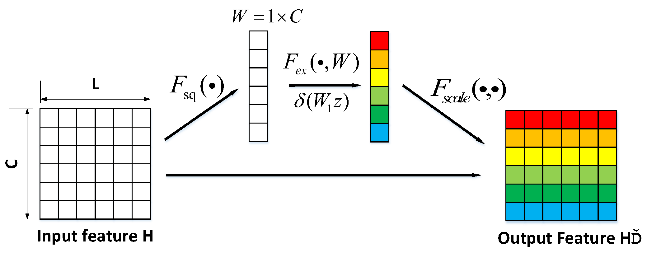
The attention mechanism filters information by adaptively weighting the features of different signal segments, highlights the fault features with important information, and suppresses irrelevant features.
The attention mechanism is shown in Figure 2. C represents the number of characteristic channels, and L represents the number of characteristic channels. F s q ( · ) is the compression operation, is the excitation operation, and F s c a l e ( · ) is the product operation. First is the compression operation. Along the direction of the feature channel, use global average pooling to compress features of size L × C into vectors of size 1 × C . There, the characteristics of each channel are compressed into a channel characteristic response value with a global receptive field.
The calculation process is as follows:
z = F s q ( H ) = 1 L i = 1 L u c ( i ) ,
where z is the output after compression, i = 1 , 2 , L , and u c ( i ) is the output value of column i in the characteristic channel c .
The second is the excitation operation. Adding two full connection layers to predict the importance of each channel to obtain the importance of different channels. The specific implementation is as follows:
y = F ex ( z ) = σ ( g ( z , W ) ) = σ ( W 2 δ ( W 1 z ) ) ,
where σ ( · ) is the sigmoid activation function, W 1 , W 2 are the weight matrix of the two fully connected layers, and δ ( · ) is the Relu activation function.
Finally, the operation is multiplication, and the channel weights obtained by the above operations are weighted to the original features channel by multiplication so as to obtain the feature sequence after attention screening. The specific implementation is as follows:
X c = F s c a l e ( U , y ) = U × y ,
When the rolling bearing has a local fault, the fault position will generate pulse excitation and resonance to other parts, which makes the vibration signal components complex. Therefore, the signal characteristics collected at different times under the same working condition are different. Some characteristics can be used to accurately diagnose the fault information, and some may cause interference, which reduces the generalization ability of the model. To focus on more discriminative features and suppress irrelevant features, this paper uses a one-dimensional attention module to obtain the weight coefficients of different features.

3. A Multi-Scale Attention Mechanism Domain Adversarial Neural Network for Bearing Fault Diagnosis

3.1. Fault Diagnosis Method Framework

The fault diagnosis method framework proposed in this paper firstly uses the multi-scale convolution structure, and this structure is used to widen the width of the network, extract sensitive features of different dimensions, and fuse the information of different scale features. Then, introduce an attention mechanism into the feature extractor to focus more on the key features, and suppress the attention of irrelevant features, thus helping to improve the accuracy of fault identification. introducing MMD into the prediction tag space for domain adaptation, measuring the difference between the distribution of the target domain and the source domain, and improving the ability of the feature extractor to extract domain invariant features. The domain discriminator distinguishes whether the data come from the target domain or the source domain, and it finally inputs the data into the classifier for fault classification.
Figure 3 shows the framework of fault diagnosis method for domain adversarial migration based on multi-scale and attention mechanism, which is mainly composed of four parts: a feature extractor, based on multi-scale and attention mechanism, as well as a domain discriminator, a feature classifier, and a category domain adaptation design, based on the maximum mean discrepancy.
The feature extractor is composed of three layers of one-dimensional convolutional neural networks with different scales and an attention mechanism embedded in residual blocks. Introduce an attention mechanism into the feature extractor to focus on more useful features and to suppress irrelevant features.
The classification module is composed of the full connection layer. The fault features extracted by the feature extractor are classified by the softmax layer. The domain recognition module is composed of two fully connected neural network layers. The category domain adaptation design uses the MMD distance as the target loss function.
In the process of model training, the function of the feature extractor is to extract the common features of the target domain data and the source domain data. The function of the domain discriminator is to distinguish whether the data are from the target domain or the source domain. The function of the feature classifier is to correctly classify the fault signal. The class domain adaptation design is to reduce the difference in the distribution of the source domain and the target domain data in the prediction tag space and improve the ability of the feature extractor to extract domain invariant features.

3.2. Feature Extraction Method Based on a Multi-Scale Module and an Attention Mechanism

The feature module includes a multi-scale module and an attention mechanism. There are three convolution modules with different scales in the multi-scale module. First, in the convolution module of the first scale, the input data are convoluted as follows:
x i 1 z = δ 1 ( x i z 1 × ω 1 z + b 1 z ) ,
In the convolution module of the second scale, the input data are convoluted as follows:
x i 2 z = δ 2 ( x i z 1 × ω 2 z + b 2 z ) ,
In the convolution module of the third scale, the input data are convoluted as follows:
x i 3 z = δ 3 ( x i z 1 × ω 3 z + b 3 z ) ,
Then, the features extracted from the three scales are fused:
x i z = x i 1 z + x i 2 z + x i 3 z ,
where x i z 1 represents the output of the previous convolution module of the data, x i z represents the output of the current convolution module of the data, z represents the convolution module, ω z and represents the parameters in each convolution calculation, and δ ( · ) represents the activation function.
Then, x i z inputs the residual block in the attention module to extract the deep abstract representation of the set features, and the formula is as follows:
x i z + 1 = x i z + j = 1 L ( F ( x i z , j , W j ) ) ,
where x i z + 1 is the output of the residual block, W j is the weight matrix of each residual block, L is the number of residual blocks, and F is the residual map to be learned. Then, give different weights to the characteristics of different channels. First, perform global average pooling on input x i z , and the results are as follows:
v m z = G A P ( x i z ) = 1 L n = 1 L x i , m z ( n ) ,
where m represents the mth channel in x i z , and the feature vectors obtained through the two fully connected layers are used to adjust x i z , and the adjusted x i z is:
x i z = x i z + v m z × x i z ,
G ( x i s , θ f ) = x i s ,
G ( x i t , θ f ) = x i t ,
where x i s and x i t in the above expression represent feature outputs of the source domain data and the target domain data after the feature extractor.

3.3. Design of Feature Classifier

The fault diagnosis classification module is composed of a full connection layer. The source domain features extracted by the feature module are input to the fault diagnosis module. The formula is as follows:
x i s , f c = δ ( x i s ; θ f c ) = σ ( ω f × x i s + b f )
where θ f c = { ω f c , b f c } is the parameter of the full connection layer, σ ( · ) is the activation function, and x i s is the source domain feature.
The softmax function is selected as the label prediction, and its output is the probability of each type of sample. The formula is as follows:
h i s = [ p ( y i s = 0 | x i s , f c ) p ( y i s = 5 | x i s , f c ) ] ,
The loss of the fault classifier is:
L y ( x i s ) = 1 n s i = 1 n s L y i ( x i s , f c , y i s ) ,
L y i ( x i s , f c , y i s ) = P i s log 1 G y ( G f ( x i s ) ) , y i s ) ,
where P i s represents 0 or 1. If the true category of sample i is equal to s, take 1, otherwise take 0. y i is the label of the bearing, G f ( x i s ) is the output of the ith source domain sample mapped by the feature extractor, n s is the number of samples, and G y ( · ) is the output of the classifier.

3.4. Design of Domain Discriminator

In the domain classification, the feature extraction is performed on the target domain data using the Formulas (16)–(22) to obtain the feature output, which is then input to the full connection layer of the domain discriminator. The formula is as follows:
x i t , f c = δ ( x i t ; θ f c ) = σ ( ω f × x i t + b f ) ,
Obtain x i t , f c . It is a binary classification problem to consider whether the data comes from the source domain or the target domain at the output layer. The formula is as follows:
L d = 1 n s i = 1 n s L d i ( x i s , f c ) + 1 n t j = 1 n t L d j ( x j t , f c ) ,
L d i ( x i ) = L d ( G d ( G f ( x i ) ) , d i ) = d i log 1 G d ( G f ( x i ) ) + ( 1 d i ) log 1 G d ( G f ( x i ) ) ,
where n s is the number of samples in the source domain, n t is the number of samples in the target domain, and G d ( · ) is the output of the domain classification module.

3.5. Class Domain Adaptation Design Based on the Maximum Mean Difference

The category domain adaptation design is to reduce the difference between the data distribution of the source domain and the target domain in the predicted tag space, improve the ability of the feature extractor to extract domain invariant features, calculate the MMD distance between the distribution of the source domain and the target domain in the tag space, take it as the objective loss function of the category field adaptation, and use the MMD distance loss to minimize the difference in the conditional distribution between the source domain and the target domain.
The formula is as follows:
L M M D = 1 n s n s i = 1 n s j = 1 n s k ( x i s , x j s ) + 1 n t n t i = 1 n t j = 1 n t k ( x i t , x j t ) 2 n s n t i = 1 n s j = 1 n t k ( x i s , x j t ) ,

3.6. Total Loss Function Design

Because a gradient reversal layer is added between the domain discriminator and the feature extractor, the gradient that is transmitted to the feature extractor G f during the backpropagation of L d is λ L d θ f . At this time, G f optimization will increase the error of the domain discriminator, and the parameter θ f is learned by maximizing the loss function L d of the domain discriminator, while the gradient in the domain discriminator G d is L d θ d , and the parameter θ d is learned by minimizing the loss function L d of the domain discriminator. The overall loss function includes three parts: the feature classification loss function in Formula (27), the domain classification loss function of Formula (30), and the category domain adaptation loss function of Formula (32). So, the overall loss function is:
L ( θ f , θ y , θ d ) = L y ( x i s ) - λ 1 L d + λ 2 L MMD = 1 n s i = 1 n s L y i ( x i s ) λ 1 n s i = 1 n s L d i ( x i s , f c ) λ 1 n t j = 1 n t L d j ( x i t , f c ) + λ 2 n s n s i = 1 n s j = 1 n s k ( x i s , x j s ) + λ 2 n t n t i = 1 n t j = 1 n t k ( x i t , x j t ) 2 λ 2 n s n t i = 1 n s j = 1 n t k ( x i s , x j t )
The optimization parameters are as follows:
θ ^ f , θ ^ y = arg min L ( θ f , θ y , θ d ) θ f , θ y ,
θ ^ d = arg min L ( θ ^ f , θ ^ y , θ d ) θ d ,
where θ f , θ d , θ y , respectively, represent parameters in the feature extraction module, the domain classification module, and the fault diagnosis classification module.

3.7. Algorithm Flow

Figure 4 introduces the process of the fault diagnosis model proposed in this paper, mainly including three parts: data processing, training process, and testing process. The specific steps are as follows:
(1)
The bearing vibration data under different working conditions are collected and normalized, and then they are converted into frequency–domain signals using fast Fourier transform as input, which is divided into source domain data X s = { x s i , y s i } n s i = 1 and target domain data X t = { x t i } n t i = 1 . Finally, the source domain data is divided into two parts: the verification set and the training set, and the target domain data is divided into two parts: the test set and the training set.
(2)
The training sets of the source domain data and the target domain data are input into the shared multi-scale feature extractor, and the source domain multi-scale features x i 1 s , x i 2 s , x i 3 s and the target domain multi-scale features x i 1 t , x i 2 t , x i 3 t are extracted, respectively, via Equations (16)–(18). Additionally, use Formula (19) to fuse the multi-scale features of the source domain and the target domain to obtain x i s , x i t . Through the attention mechanism, the source domain feature x i s and the target domain feature x i t , with more discriminative power, are extracted through Formulas (20)–(22), and the feature x i s extracted from the source domain is input to the feature classifier for classification. The classification loss L y ( x i s ) is calculated by Formulas (25) and (27), and then the features extracted from the source domain and the target domain are input to the category domain adapter to calculate the MMD loss L M M D by Formula (32), and the domain discriminator is used to calculate the domain discriminator loss L d by Formulas (29) and (30), and the three loss functions are constructed into a total loss function L ( θ f , θ y , θ d ) . Finally, the model is iteratively trained to minimize the classification loss and MMD loss and maximize the domain discriminator loss.
(3)
The model is tested, and the target domain test set is input into the feature extractor and classifier for actual fault diagnosis to test the effectiveness of diagnosis.

4. Application Results and Analysis

4.1. Case Western Reserve University Bearing Data Analysis

4.1.1. Data Preparation

In this paper, the rolling bearing data set of Case Western Reserve University (CWRU) is used for verification. The download link is http://engineering.case.edu/bearingdatacenter/ (accessed on 10 October 2021). The sampling frequency of the selected data is 12 kHz. The bearings used are divided into a normal state, inner ring fault, outer ring fault, and rolling element fault. As shown in Figure 5, the test bed uses EDM technology to arrange single point faults on the inner ring, rolling element, and outer ring (three o’clock direction) of the bearing. The faults at each position have different fault degrees. The fault diameters are 0.007 inches, 0.014 inches, and 0.021 inches, respectively. Figure 5 is from the bearing data center of the Case School of Engineering.
Three different load states of sample data were selected: 1HP (1772 r/min), 2HP (1750 r/min), and 3HP (1730 r/min), which were divided into three data sets: A, B, and C. An amount of 2048 data points of normal bearing vibration data of Western Reserve University and vibration data of inner ring, rolling element, and outer ring fault are selected as a sample. Table 1 shows the composition of experimental samples. Six transmission tasks are set: A B, C, B A, C, C A, B. An amount of 300 samples are collected for each faulty bearing state, of which 200 are training samples, and 100 are test samples. Each transmission task is performed five times to take the average value. When the motor load changes, speed will slightly shift. It is a fast process.

4.1.2. Performance Comparison and Analysis of Different Algorithms

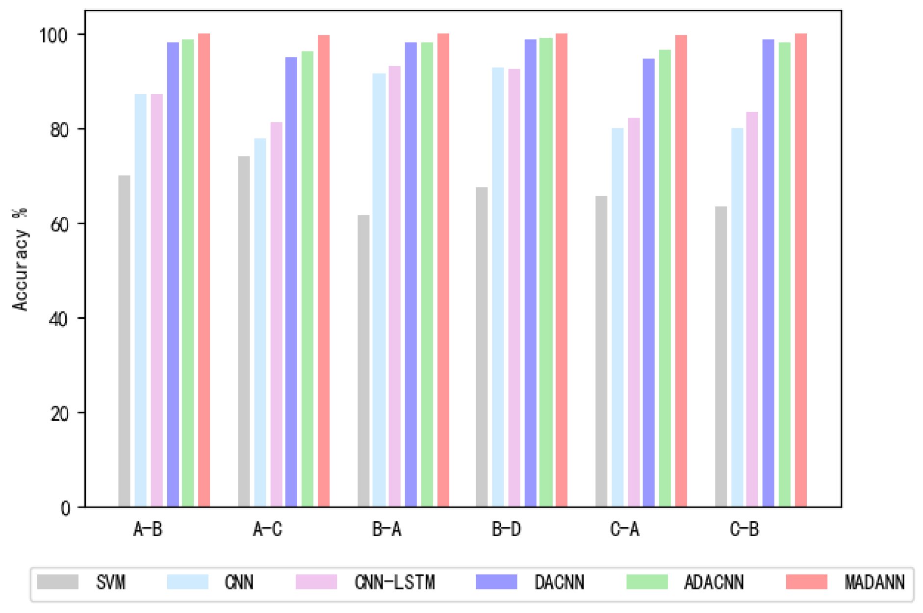
To confirm the advantages of the proposed fault diagnosis method (Figure 3) under variable operating conditions (loads), the shallow model, the deep model, and the domain adaptive model are selected for comparative experiments, which are SVM, CNN, CNN-LSTM, DACNN, and ADACNN, respectively. (1) SVM extracts ten time–domain features and three frequency–domain features, and then it inputs them into SVM for fault diagnosis under variable conditions. (2) CNN uses a three-layer convolution pooling layer for feature extraction, sends it to the softmax layer for fault diagnosis, and then uses the target domain test set for migration testing of the trained model. The sample size of each operating condition is 3000, and each health state includes 200 training samples and 100 test samples. (3) CNN-LSTM adds an LSTM layer based on CNN to capture the long-term dependence between time series data. The sample size of each operating condition is 3000, and each health state includes 200 training samples and 100 test samples. (4) The DACNN method proposed in document 35 extracts the common features of the source domain and the target domain through a discriminant classifier, uses adversarial learning, and finally inputs the test set of the target domain into the classifier for classification. The sample size of each operating condition is 2000, and each health state includes 100 training samples and 100 test samples. (5) The ADACNN method proposed in document 31 uses MMD distance to measure the difference between the distribution of the target domain and the source domain. The structure of the feature extractor, classifier, and domain discriminator is the same as DACNN. The sample size of each operating condition is 3000, and each health state includes 200 training samples and 100 test samples. Table 2 and Figure 6 show the results obtained by the above method.
It can be concluded, from Table 2 and Figure 6, that: (1) the generalization ability of conventional shallow models, such as SVM, is poor under variable load conditions. (2) For a single depth model, such as CNN and CNN-LSTM, superimposed by two depth models, the average accuracy rate of fault identification is only 84.9% and 86.7%, respectively, when the operating conditions change. Because the change in data distribution has a significant impact on the depth model, the classification effect is poor, which also reveals the importance of reducing the distribution difference between the two fields. (4) Compared with CNN and CNN-LSTM models, the accuracy rate of DACNN is 97.2%, indicating that both feature alignment and domain adversarial learning can mitigate the impact of data distribution deviation caused by variable load conditions. (5) The accuracy rate of the ADACNN algorithm proposed in the document [29] is 97.7%, which is slightly higher than that of DACNN, indicating that introducing MMD domain adaptation into feature space and prediction tag space can alleviate the problem of algorithm performance degradation caused by the distribution deviation between test data and training data. However, the above algorithms use CNN to directly extract features, without considering more discriminative features, so the highest diagnostic accuracy is only 97.7%. In this paper, we use the attention mechanism to consider the weight of each feature extracted from the convolution layer, and then we screen out important features and use the multi-scale convolution structure to broaden the width of the network to achieve the extraction of sensitive features in different dimensions, Finally, the MMD domain is used to adaptively alleviate the problem of algorithm performance degradation caused by the difference of data distribution. The accuracy of this method is greatly improved compared with the above methods.

4.1.3. Feature Visualization and Analysis

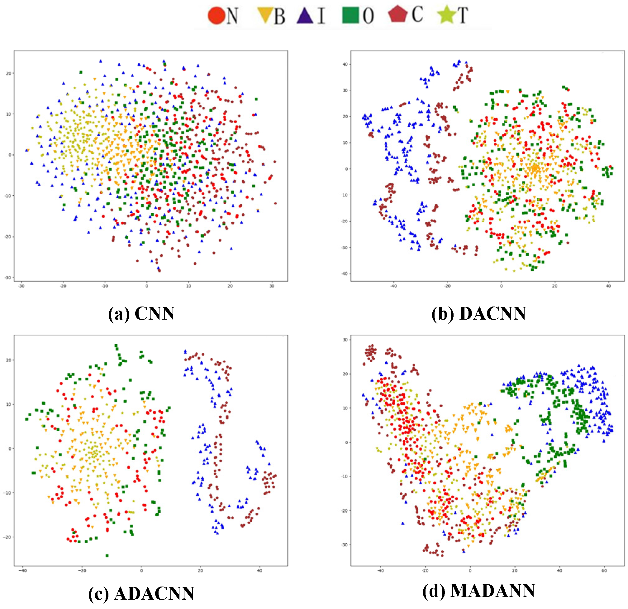
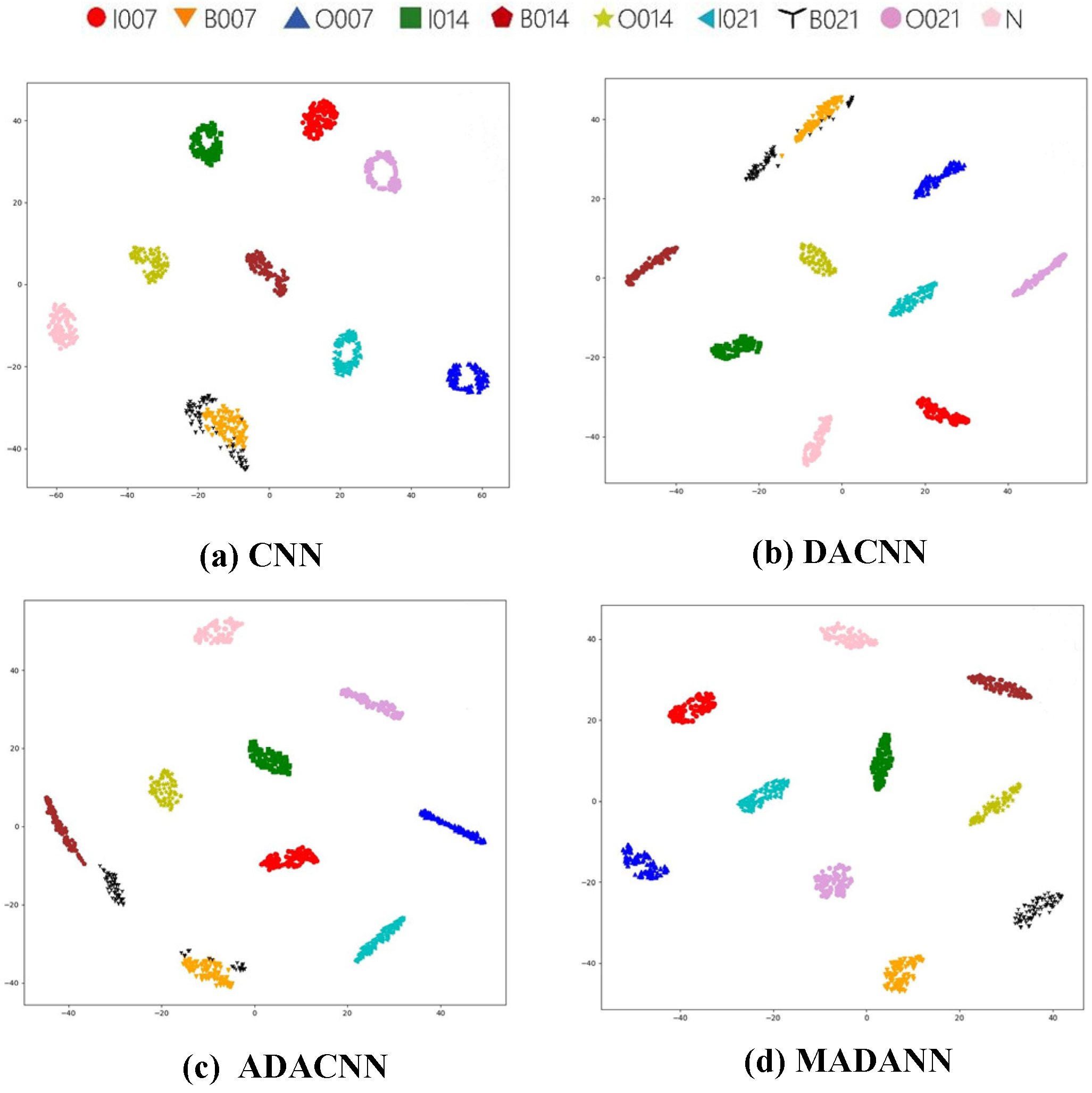
To further verify the advantages of the proposed method in fault diagnosis under variable operating conditions, CNN, DACNN, and ADACNN are used as comparisons. Taking B-C as an example, T-SNE visualization is used to analyze the last full connection layer of the classifier. The feature visualization results are shown in Figure 7 and Figure 8. Figure 7 shows the distribution of target domain sample convolution results by different models. Figure 8 shows the distribution of target domain sample features extracted by different models.
It can be analyzed from Figure 8a that, for CNN, the fault features of 0.007-inch rolling element and 0.021-inch rolling element are seriously overlapped, and it is impossible to distinguish which type of features are. Other fault features are obvious. (2) It can be analyzed, from Figure 8b,c, that the impact of data distribution shift caused by variable load conditions, forming obvious clusters, is alleviated due to the introduction of feature alignment and domain adversarial learning. Although the fault features of the 0.007-inch rolling element and the 0.021-inch rolling element are still partially overlapped, the situation is improved compared with CNN. (3) It can be seen from Figure 8d that the multi-scale convolution structure broadens the width of the network to achieve the extraction of sensitive features in different dimensions. The channel attention mechanism is introduced into the feature extractor to focus more on the key features with discriminant power, suppress the attention of irrelevant features, and combine feature alignment and domain confrontation learning to extract features more suitable for classification. The fault features of the 0.007-inch rolling element and the 0.021-inch rolling element are clearly separated, and there is no aliasing. This proves, again, that the proposed fault identification method, based on MADANN, has better identification ability under different load conditions.

4.2. Data Analysis of PT500mini Mechanical Bearing Fault Simulation Test Bed

4.2.1. Data Preparation

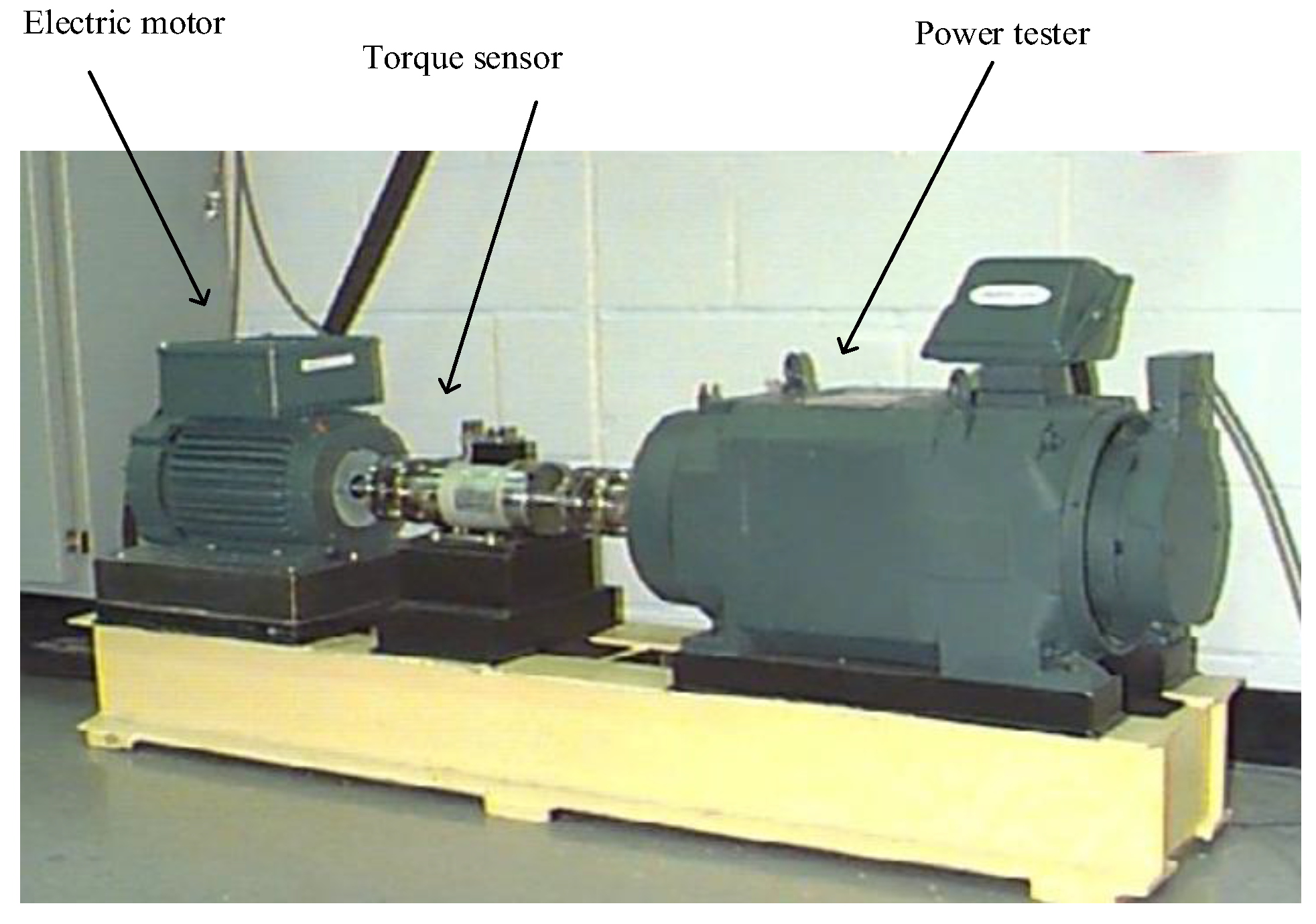
The PT500mini mechanical bearing gear fault simulation test-bed is used to simulate bearing fault and collect data. The test bed is shown in Figure 9 below. The sampling frequency of selected data is 48 kHz. The bearings used are divided into normal state (N), inner ring fault (I), outer ring fault (O), rolling element fault (B), comprehensive fault (C), and cage fault (T). The inner ring fault is an inner ring crack of 0.3 mm, the outer ring fault is an outer ring crack of 0.3 mm, the rolling element fault is a peeling pit of 3 mm, the comprehensive fault is a crack of 0.3 mm on the inner and outer rings, and the cage fault is a cage fracture.
The sample data has three different rotational speeds: 1000 r/min, 1500 r/min, and 2000 r/min, which are divided into three data sets: A, B, and C. An amount of 2048 data points of vibration data are selected as a sample, and 1000 samples are collected in each state. Among them, 700 are test sets and 300 are test sets. Table 3 below shows the composition of bearing test samples. Six transmission tasks are set: A B, C, B A, C, C A, B. Table 4 below gives the details of the experimental data set built under variable operating conditions.

4.2.2. Experimental Results and Analysis

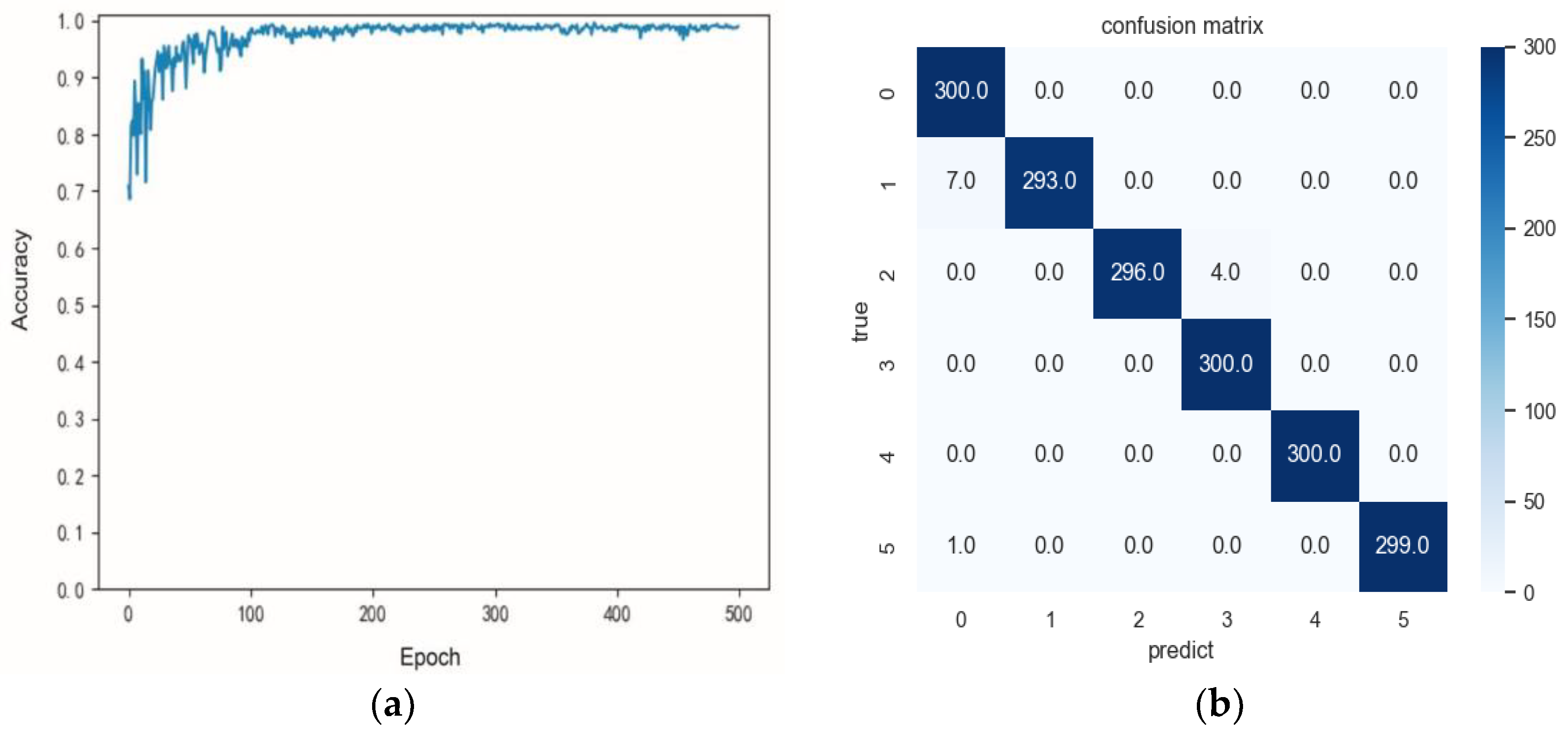
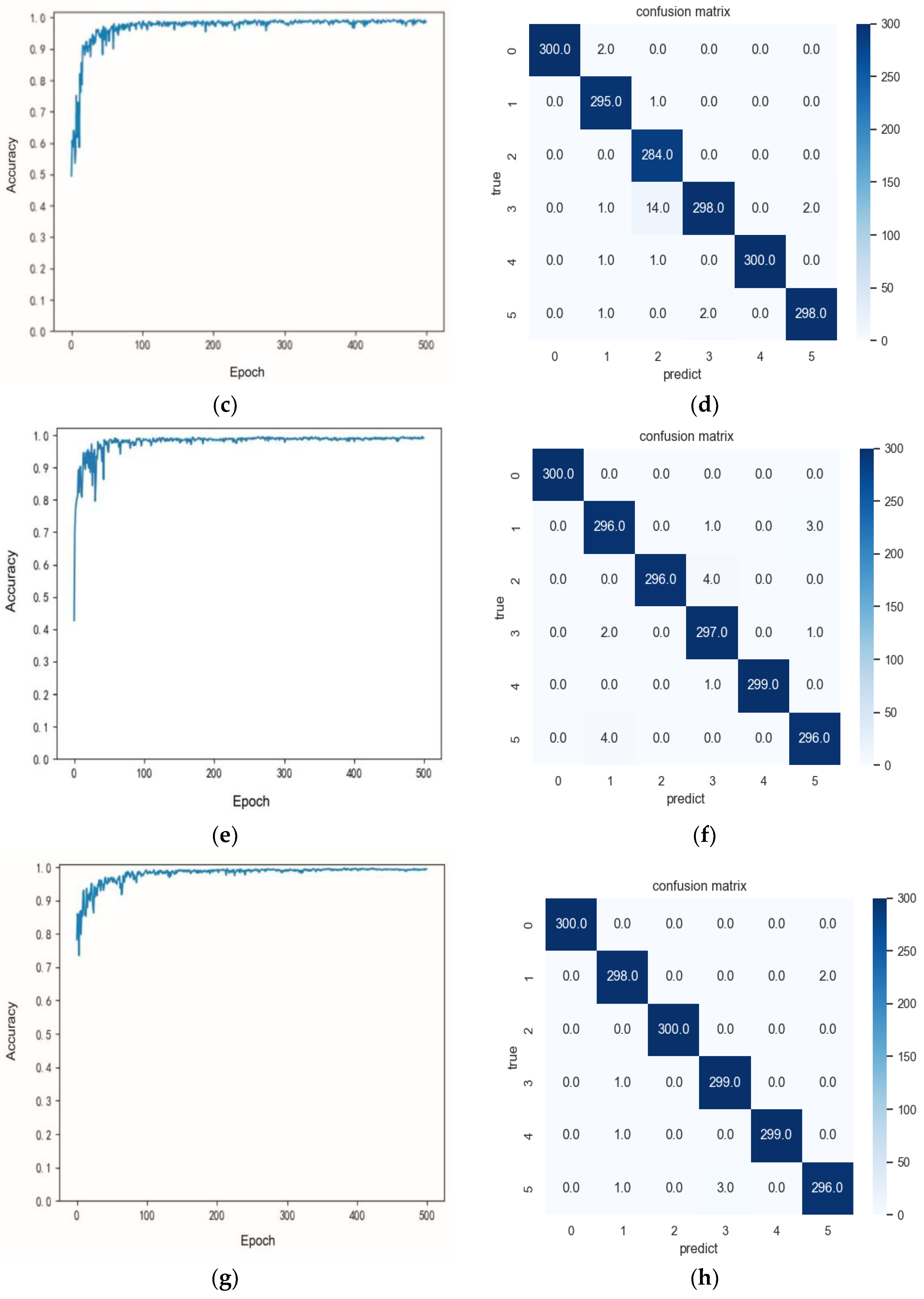
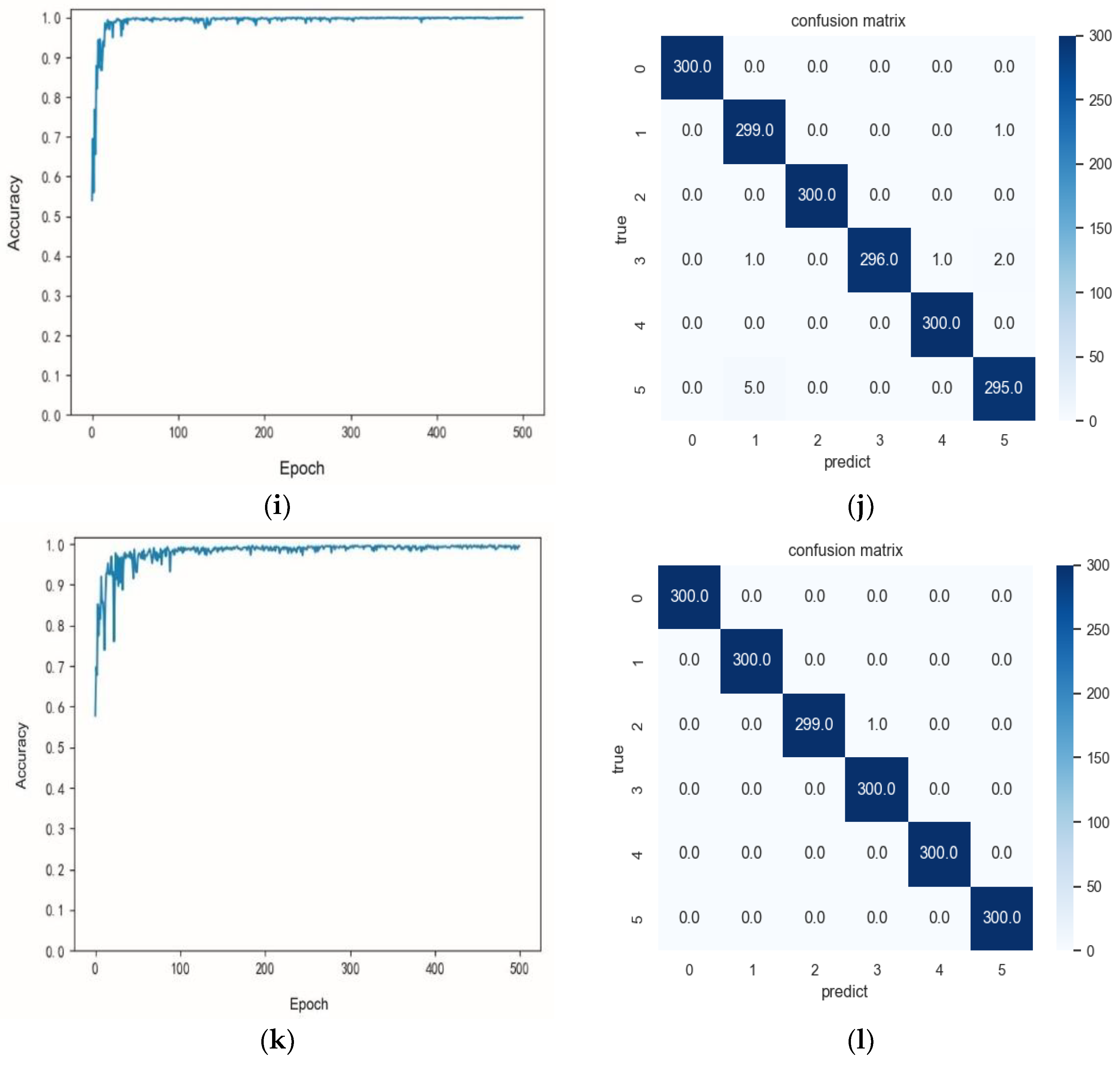
A variable load condition is a scene with a small difference in signal characteristic distribution between the source condition and the target condition. To verify the accuracy of the proposed method in the case of the large difference in distribution, the variable speed condition is selected for fault diagnosis in this paper. Figure 10 is the accuracy curve and confusion matrix of 500 iterations under each variable working condition. From the accuracy curve under each variable working condition in Figure 10, it can be seen that the accuracy of different tasks is constantly rising. Although it will decline during the iteration, it will eventually stabilize. (1) For task A-B, as shown in Figure 10a,b, it can be analyzed that the accuracy rate can reach 98.6% by the confusion matrix, and a small number of samples are misclassified. For task A-C, as shown in Figure 10c,d, it can be analyzed that the accuracy rate can reach 98.6%, which is slightly lower than that of task A-B. Because the large change in rotational speed of A-C results in a large difference in the characteristic distribution between the two working conditions, the accuracy rate is somewhat lower than that of other tasks. (2) For task B-A and B-C, as shown in Figure 10e–h, the accuracy can reach 99.1% and 99.5%, respectively. Only a small number of samples are misclassified, and the accuracy is high. For task C-A, as shown in Figure 10i,j, the accuracy can reach 99.3%. For task C-B, as shown in Figure 10k,l, the analysis accuracy is 99.9%. Only one sample is misclassified, and the accuracy is very high.

4.3. Computational Expense

This paper experimentally verifies the use of a notebook CPU AMD Ryzen 7 4800 H. The simulation takes 3193 s on the public data set and 1544 s on the PT500mini mechanical bearing fault simulation test bench data set. If the network structure is determined, the fixed structure is loaded onto the airborne chip. The judgment time of new samples is very short. It can meet the real-time requirements and conform to the actual project.

5. Conclusions

In this paper, a multi-scale attention mechanism domain adversarial neural network for bearing fault diagnosis (MADANN) is proposed, which includes a feature extractor, domain discriminator, feature classifier, and category domain adaptation design based on the maximum mean discrepancy. A feature extractor combining multi-scale and attention mechanism is designed to extract multi-scale and more discriminative features, and the source domain and the target domain are mapped to the feature space and the label prediction space. The maximum mean difference alignment is introduced into the label prediction space, and it is used to reduce the difference in data distribution between the source domain and the target domain in the prediction label space, as well as to improve the ability of the feature extractor to extract domain invariant features. Domain adversarial learning is introduced between the domain discriminator and feature extractor, and it is used to realize feature domain adaptation. For the variable load problem, this paper uses the open data set to verify that the accuracy of the proposed method is better than other methods. For the variable speed problem, this paper uses the data set collected from the mechanical bearing fault simulation test bed to verify that the proposed method also has high accuracy. The results of case analysis show that the method proposed in this paper can accurately diagnose faults in the case of no label in the target domain, variable load, and variable speed, and it is more suitable for engineering practice.
However, the method proposed in this paper does not consider the following situations: (1) under the actual variable working conditions of rolling bearings, the target working conditions will generate new faults that have never occurred under the source working conditions, and how to diagnose the new faults have not been considered. (2) There is a problem of data imbalance between the source domain samples and the target domain samples. Serious data imbalance will lead to a strong imbalance in the distribution of fault samples, and how to diagnose the imbalance samples is not considered. In the future, in view of the above two problems, relevant research will be carried out on how to accurately classify new faults under variable conditions and how to solve the problem of data imbalance.

Author Contributions

Conceptualization, Q.Z., N.T., X.F. and C.W.; methodology, N.T. and X.F.; validation, N.T. and X.F.; formal analysis, N.T., X.F. and C.W.; resources, Q.Z. and C.W.; data curation, N.T. and X.F.; writing—original draft preparation, N.T. and X.F.; writing—review and editing, N.T., X.F. and C.W.; project administration, Q.Z.; funding acquisition, Q.Z., C.W., H.P. and C.B. All authors have read and agreed to the published version of the manuscript.

Funding

This work was supported in part by the National Key Research and Development Program of China under Grant 2021YFB3301300; in part by the National Natural Science Foundation of China under Grant 62203213; in part by the Natural Science Foundation of Jiangsu Province under Grant BK20220332; in part by the Open Project Program of Fujian Provincial Key Laboratory of Intelligent Identification and Control of Complex Dynamic System under Grant 2022A0004.

Data Availability Statement

The data used in this study are self-text and self-collection.

Conflicts of Interest

The authors declare no conflict of interest.

References

  1. Zhou, Y.; Dong, Y.; Zhou, H.; Tang, G. Deep dynamic adaptive transfer network for rolling bearing fault diagnosis with considering cross-machine instance. IEEE Trans. Instrum. Meas. 2021, 70, 3525211. [Google Scholar] [CrossRef]
  2. Chen, C.; Lu, N.; Jiang, B.; Xing, Y. A data-driven approach for assessing aero-engine health status. IFAC-Pap. Online 2022, 55, 737–742. [Google Scholar] [CrossRef]
  3. Wang, C.; Lu, N.; Cheng, Y.; Jiang, B. A data-driven aero-engine degradation prognostic strategy. IEEE Trans. Cybern. 2021, 51, 1531–1541. [Google Scholar] [CrossRef] [PubMed]
  4. Hu, Q.; Si, X.; Qin, A.; Lv, Y.; Liu, M. Balanced adaptation regularization based transfer learning for unsupervised cross-domain fault diagnosis. IEEE Sens. J. 2022, 22, 12139–12151. [Google Scholar] [CrossRef]
  5. Lei, Y.; Yang, B.; Jiang, W.; Jia, F.; Li, N.; Nandi, A.K. Applications of machine learning to machine fault diagnosis: A review and roadmap. Mech. Syst. Signal Process. 2020, 138, 106578. [Google Scholar] [CrossRef]
  6. Su, K.; Liu, J.; Xiong, H. A multi-level adaptation scheme for hierarchical bearing fault diagnosis under variable working conditions. J. Manuf. Syst. 2022, 64, 251–260. [Google Scholar] [CrossRef]
  7. Zhang, S.; Zhang, S.; Wang, B.; Habetler, T.G. Deep learning algorithms for bearing fault diagnostics–a comprehensive review. In Proceedings of the 2019 IEEE 12th International Symposium on Diagnostics for Electrical Machines, Power Electronics and Drives (SDEMPED), Paris, France, 27–30 August 2019. [Google Scholar]
  8. Xu, J.; Tong, S.; Cong, F.; Zhang, Y. The application of time–frequency reconstruction and correlation matching for rolling bearing fault diagnosis. ARCHIVE Proc. Inst. Mech. Eng. Part C J. Mech. Eng. Sci. 2015, 229, 33291–33295. [Google Scholar] [CrossRef]
  9. Zheng, J.; Cao, S.; Pan, H.; Ni, Q. Spectral envelope-based adaptive empirical Fourier decomposition method and its application to rolling bearing fault diagnosis. ISA Trans. 2022, 129, 476–492. [Google Scholar] [CrossRef]
  10. Wang, Z.; Zhang, Q.; Xiong, J.; Xiao, M.; Sun, G.; He, J. Fault diagnosis of a rolling bearing using wavelet packet denoising and random forests. IEEE Sens. J. 2017, 17, 5581–5588. [Google Scholar] [CrossRef]
  11. Li, H.; Liu, T.; Wu, X.; Chen, Q. An optimized VMD method and its applications in bearing fault diagnosis. Measurement 2020, 166, 108185. [Google Scholar] [CrossRef]
  12. Liu, S.; Sun, Y.; Zhang, L. A novel fault diagnosis method based on noise-assisted MEMD and functional neural fuzzy network for rolling element bearings. IEEE Access 2018, 6, 27048–27068. [Google Scholar] [CrossRef]
  13. Goyal, D.; Dhami, S.; Pabla, B. Non-contact fault diagnosis of bearings in machine learning environment. IEEE Sens. J. 2020, 20, 4816–4823. [Google Scholar] [CrossRef]
  14. Zuo, L.; Xu, F.; Zhang, C.; Xiahou, T.; Liu, Y. A multi-layer spiking neural network-based approach to bearing fault diagnosis. Reliab. Eng. Syst. Saf. 2022, 225, 108561. [Google Scholar] [CrossRef]
  15. Wang, Z.; Yao, L.; Cai, Y. Rolling bearing fault diagnosis using generalized refined composite multiscale sample entropy and optimized support vector machine. Measurement 2020, 156, 107574. [Google Scholar] [CrossRef]
  16. Tan, H.; Xie, S.; Liu, R.; Ma, W. Bearing fault identification based on stacking modified composite multiscale dispersion entropy and optimised support vector machine. Measurement 2021, 186, 110180. [Google Scholar] [CrossRef]
  17. Wang, Z.; Yao, L.; Chen, G.; Ding, J. Modified multiscale weighted permutation entropy and optimized support vector machine method for rolling bearing fault diagnosis with complex signals. ISA Trans. 2021, 114, 470–484. [Google Scholar] [CrossRef]
  18. Lu, C.; Wang, Z.; Zhou, B. Intelligent fault diagnosis of rolling bearing using hierarchical convolutional network based health state classification. Adv. Eng. Inform. 2017, 32, 139–151. [Google Scholar] [CrossRef]
  19. Gao, S.; Pei, Z.; Zhang, Y.; Li, T. Bearing fault diagnosis based on adaptive convolutional neural network with Nesterov Momentum. IEEE Sens. J. 2021, 21, 9268–9276. [Google Scholar] [CrossRef]
  20. Wang, Y.; Ding, X.; Zeng, Q.; Wang, L.; Shao, Y. Intelligent rolling bearing fault diagnosis via vision ConvNet. IEEE Sens. J. 2021, 21, 6600–6609. [Google Scholar] [CrossRef]
  21. Sun, J.; Wen, J.; Yuan, C.; Liu, Z.; Xiao, Q. Bearing fault diagnosis based on multiple transformation domain fusion and improved residual Dense Networks. IEEE Sens. J. 2022, 22, 1541–1551. [Google Scholar] [CrossRef]
  22. Sadoughi, M.; Hu, C. Physics-Based convolutional neural network for fault diagnosis of rolling element bearings. IEEE Sens. J. 2019, 19, 4181–4192. [Google Scholar] [CrossRef]
  23. Udmale, S.; Singh, S.; Singh, R.; Sangaiah, A.K. Multi-Fault bearing classification using sensors and ConvNet-Based transfer learning approach. IEEE Sens. J. 2020, 20, 1433–1444. [Google Scholar] [CrossRef]
  24. Liu, D.; Cui, L.; Cheng, W.; Zhao, D.; Wen, W. Rolling bearing fault severity recognition via data mining integrated with convolutional neural network. IEEE Sens. J. 2022, 22, 5768–5777. [Google Scholar] [CrossRef]
  25. Lu, S.; Qian, G.; He, Q.; Liu, F.; Liu, Y.; Wang, Q. In situ motor fault diagnosis using enhanced convolutional neural network in an embedded system. IEEE Sens. J. 2020, 20, 8287–8296. [Google Scholar] [CrossRef]
  26. Li, G.; Wu, J.; Deng, C.; Chen, Z. Parallel multi-fusion convolutional neural networks based fault diagnosis of rotating machinery under noisy environments. ISA Trans. 2021, 128, 545–555. [Google Scholar] [CrossRef]
  27. Wang, H.; Liu, Z.; Peng, D.; Qin, Y. Understanding and learning discriminant features based on multi-attention 1DCNN for wheelset bearing fault diagnosis. IEEE Trans. Ind. Inform. 2020, 16, 5735–5745. [Google Scholar] [CrossRef]
  28. Guo, X.; Chen, L.; Shen, C. Hierarchical adaptive deep convolution neural network and its application to bearing fault diagnosis. Measurement 2016, 93, 490–502. [Google Scholar] [CrossRef]
  29. Magar, R.; Ghule, L.; Li, J.; Zhao, Y.; Farimani, A.B. FaultNet: A Deep Convolutional Neural Network for bearing fault classification. IEEE Access 2021, 9, 25189–25199. [Google Scholar] [CrossRef]
  30. Wang, Q.; MiChau, G.; Fink, O. Domain adaptive transfer learning for fault diagnosis. In Proceedings of the 2019 Prognostics and System Health Management Conference (PHM-Paris), Paris, France, 2–5 May 2019. [Google Scholar]
  31. Li, J.; Huang, R.; He, G.; Wang, S.; Li, G.; Li, W. A deep adversarial transfer learning network for machinery emerging fault detection. IEEE Sens. J. 2020, 20, 8413–8422. [Google Scholar] [CrossRef]
  32. Lu, N.; Xiao, H.; Sun, Y.; Han, M.; Wang, Y. A new method for intelligent fault diagnosis of machines based on unsupervised domain adaptation. Neurocomputing 2021, 427, 96–109. [Google Scholar] [CrossRef]
  33. Wu, Y.; Zhao, R.; Ma, H.; He, Q.; Du, S.; Wu, J. Adversarial domain adaptation convolutional neural network for intelligent recognition of bearing faults. Measurement 2022, 195, 111150. [Google Scholar] [CrossRef]
  34. Wu, Z.; Zhang, H.; Guo, J.; Ji, Y.; Pecht, M. Imbalanced bearing fault diagnosis under variant working conditions using cost-sensitive deep domain adaptation network. Expert Syst. Appl. 2022, 193, 116459. [Google Scholar] [CrossRef]
  35. Liu, Y.; Shi, K.; Li, Z.; Ding, G.F.; Zou, Y.S. Transfer learning method for bearing fault diagnosis based on fully convolutional conditional Wasserstein adversarial Networks. Measurement 2021, 180, 109553. [Google Scholar] [CrossRef]
  36. Zou, Y.; Liu, Y.; Deng, J.; Jiang, Y.; Zhang, W. A novel transfer learning method for bearing fault diagnosis under different working conditions. Measurement 2021, 171, 108767. [Google Scholar] [CrossRef]
  37. Wu, Z.; Jiang, H.; Liu, S.; Yang, C. A Gaussian-guided adversarial adaptation transfer network for rolling bearing fault diagnosis. Adv. Eng. Inform. 2022, 53, 101651. [Google Scholar] [CrossRef]
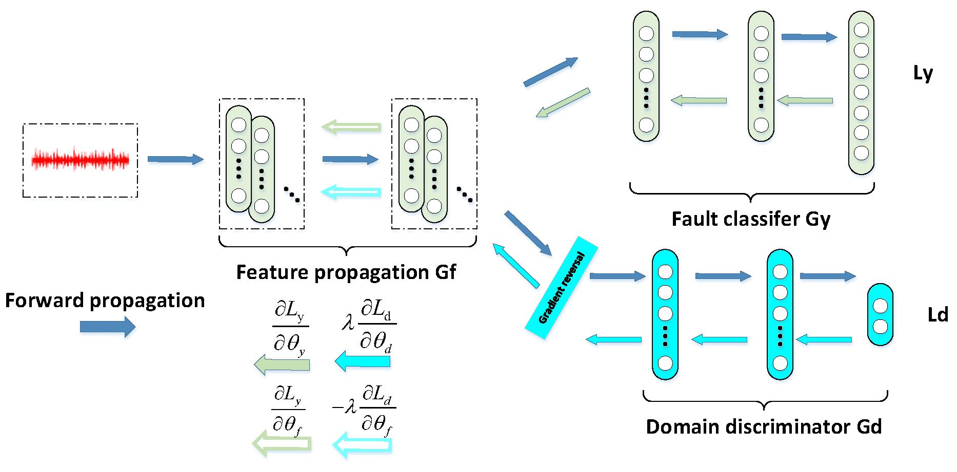
Figure 1. DANN network.
Actuators 12 00188 g001
Figure 2. Attention mechanism.
Actuators 12 00188 g002
Figure 3. Fault diagnosis method framework.
Actuators 12 00188 g003
Figure 4. Fault diagnosis model process.
Actuators 12 00188 g004
Figure 5. Case Western Reserve University bearing testing rig.
Actuators 12 00188 g005
Figure 6. Comparison of accuracy of different algorithms.
Actuators 12 00188 g006
Figure 7. T-SNE visualization of convolution results.
Actuators 12 00188 g007
Figure 8. T-SNE visualization of different models.
Actuators 12 00188 g008
Figure 9. PT500mini mechanical bearing gear fault simulation test bed.
Actuators 12 00188 g009
Figure 10. Accuracy curve and confusion matrix of 500 iterations under different tasks: (a,b) Task A-B accuracy curve and confusion matrix; (c,d) Task A-C accuracy curve and confusion matrix; (e,f) Task B-A accuracy curve and confusion matrix; (g,h) Task B-C accuracy curve and confusion matrix; (i,j) Task C-A accuracy curve and confusion matrix; (k,l) Task C-B accuracy curve and confusion matrix.
Actuators 12 00188 g010aActuators 12 00188 g010bActuators 12 00188 g010c
Table 1. Composition of experimental samples.
TypeLengthQuantityLabel
Normal20483009
Inner ring fault (0.007 inch)20483000
Rolling element failure (0.007 inch)20483001
Outer ring fault (0.007 inch)20483002
Inner ring fault (0.014 inch)20483003
Rolling element failure (0.014 inch)20483004
Outer ring fault (0.014 inch)20483005
Inner ring fault (0.021 inch)20483006
Rolling element failure (0.021 inch)20483007
Outer ring fault (0.021 inch)20483008
Table 2. Average accuracy of different algorithms.
MethodsA-BA-CB-AB-CC-AC-BAverage
SVM707461.667.665.763.367.0
CNN87.377.891.592.780.079.984.9
CNN-LSTM87.381.493.192.682.283.486.7
DACNN98.195.19898.894.698.797.2
ADACNN98.696.29899.296.69897.7
MADANN99.999.799.910099.810099.8
Table 3. Composition of experimental samples.
Sample TypeSample LengthNumber of SamplesCategory Tag
N204810000
B204810001
C204810002
I204810003
O204810004
T204810005
Table 4. Transmission tasks.
Domain AdaptationSource DomainTarget DomainAccuracy
A-B1000 r/min1500 r/min99.1
A-C1000 r/min2000 r/min98.6
B-A1500 r/min1000 r/min99.1
B-C1500 r/min2000 r/min99.5
C-A2000 r/min1000 r/min99.3
C-B2000 r/min1500 r/min99.9
Disclaimer/Publisher’s Note: The statements, opinions and data contained in all publications are solely those of the individual author(s) and contributor(s) and not of MDPI and/or the editor(s). MDPI and/or the editor(s) disclaim responsibility for any injury to people or property resulting from any ideas, methods, instructions or products referred to in the content.