An Enhanced Navigation Algorithm with an Adaptive Controller for Wheeled Mobile Robot Based on Bidirectional RRT

Abstract

A navigation algorithm providing motion planning for two-wheeled mobile robots is proposed in this paper. The motion planning integrates path planning, velocity planning and controller design. Bidirectional rapidly-exploring random trees algorithms (RRT) with path pruning and smoothing mechanism are firstly used to obtain a collision-free path to the robot destination with directional continuity. Secondly, velocity planning based on trapezoidal velocity profile is used in both linear and angular velocities, but the position error of the endpoint of the curve appears due to the coupling problem of the nonlinear system. To reduce the error, an approximation method is used to gradually modify several parts of time length of the trapezoidal velocity profile, so the continuity of the path can still be maintained. Thirdly, the controller keeping the robot on the planned path and velocity is designed based on the dynamic model of the robot. The parameters of this controller are estimated by the adaptive low, and the gain of controller is dynamic adjusted by fuzzy logic control to avoid the case that the control value is saturated. The controller stability and the convergence of tracking error is guaranteed by Lyapunov theory. Simulation results are presented to illustrate the effectiveness and efficiency.

1. Introduction

In the past years, many studies of wheeled mobile robots have been presented. Among them, the differential wheel type mobile robot is still the most important development project in the indoor flat environment because of its flexibility and cost advantages. Common applications include unmanned factories [1], automated warehouses, and home sweeping robots [2]. Robot navigation is the basic ability to realize application functions, and path planning is the most important ability. A* algorithm is one of most representative algorithms for path planning because of its best priority search and heuristic exploration strategy to obtain good application value in most cases [3,4]. However, the exponential growth of time and space complexity makes it difficult to be applied to large or high-dimensional maps. Relatively, those algorithms with only probabilistic completeness, such as RRT algorithms, are usually able to complete path planning tasks in less time, but it is also difficult to ensure optimality and requires subsequent improvement measures [5,6,7,8]. Therefore, this paper improves the traditional RRT algorithm and designs a series of optimization mechanisms to improve the path quality and solve the problems faced by the traditional RRT algorithm.

Although path planning provides a feasible solution to the goal point, there may be some unexpected situations, such as moving obstacles overlapping the path, so that the robot cannot proceed along the predetermined path. In addition, the robot itself will deviate from the predetermined path due to some disturbances or uncertainties, so a good controller is needed to correct the state error of the robot, such as PID, feedback linearization, backstepping, sliding mode control, neural networks, and the hybrids of the above controllers [9,10,11,12]. According to the level of the controllers, they can be classified into two types, depending on the controller designed with only kinematic [13,14,15,16] or both kinematic and dynamic methods [17,18]. Generally, the former is much more simple but still enough for general cases and suitable for those motors with the ability to control velocity already. The latter is applied to high-speed cases where accuracy is required, but it requires more computing.

At the only-kinematic level, there are some research studies that have improved existing controllers. For instance, Simon X. Yang et al. [13] proposed a controller based on bioinspired neurodynamics, which can produce smooth continuous robot control signals with zero initial velocities. Thanks to the continuity of velocities, the robot reduces the overshoot at startup. Sašo Blažič [14] proposed a periodic controller, which let the convergence of the orientation error be 2kπ or kπ with k being an integer constant for different condition instead of zero. Thus, there is no need for excessive rotation of the mobile robots in the case that the initial orientation error is large. Sašo Blažič also proposed a controller design role to determine a suitable control law. Many controllers can be obtained by following this design role. Zhong-Ping Jiang et al. [15] proposed one local and one global backstepping controller for path tracking. Limiting of the denominator may be zero, and the local controller is only for small initial errors. This problem is solved in global controllers by choosing a different way for the convergence path. In this study, the global controller also expands to a very simple dynamic model.

At both kinematic and dynamic levels, Bong Seok Park [17] proposed an adaptive controller with dynamic surface control and parameter estimators. The dynamic also includes motors, and all system parameters are obtained by the four update laws estimator. Chih-Lyang Hwang [18] proposed hierarchical variable structure tracking control for car-like mobile robots. The control output is composed of equivalent and switching parts. Instead of using the PID controller of kinematic errors as the only surface to be the input of the switch function, it also considers the dynamic errors and virtual reference as the second surface so that the system has better performance against disturbances. However, saturation problems of the controller output, which are not considered in most controller designs, may become more serious, especially in the high-speed or large-initial-error cases. When the controller output is saturated, the system stability and the convergence of errors guaranteed by Lyapunov theory is invalid, which means the system may diverge. One way to avoid this is reducing the controller gain, although doing so reduces the transient response. Thus, Xiaohan Chen [16] proposed a controller with diamond-shaped input constraints to guarantee the control value is limited by the input constraints. However, this controller only works in kinematic models. To solve this, we introduce a dynamic gain adjustment [19] considering the system errors and current output based on fuzzy logic control. Once the output is saturated, the controller gain reduces automatically, and then a limited increase of the gain occurs if it finds that there is still room to increase the amount of control. By adjusting the gain, the system can still have a good transient response when solving the saturation problem.

This paper is derived from the short conference paper published in [20]. In the initial conference paper, we focused on the controller design only. This paper extends the previous research and integrates the path planning as a reference signal to the controller, which finally enables the robot to follow the predetermined path to the destination. This paper is organized as follows. The problem statement is proposed in Section 2. Path planning is proposed in Section 3. The controller design and its stability analysis are presented in Section 4. Experimental results and conclusion are proposed in Section 5 and Section 6, respectively.

2. Problem Statement

2.1. Definition of Environment and Robot

It is assumed that the robot moves on a known and bounded two-dimensional plane, which is discretized into a grid map. Each grid point corresponds to a small area of actual space. If the space in this area is completely passable, its state is regarded as free, otherwise it is regarded as occupied. The structure of wheeled mobile robot with two actuated wheels on left and right sides is shown in Figure 1. P_c is the center of mass of mobile robot. Q is the middle point of two actuated wheels. d is the distance between P_c and Q. R is the half width from left to right actuated wheel. r is the radius of the wheel. R_o is the radius of the smallest circle with its center Q that covers the entire robot. The three variables related to robot coordinates are as follows. θ is the heading angle of mobile robot. x and y are the coordinates of Q. If the wheels are non-slipping, then the nonholonomic constraint is given as:

$$\dot{x}\sin \theta -\dot{y}\cos \theta =0$$

(1)

The kinematic model of mobile robots is given in (2). q = [x, y, θ]^T is the vector of position. z = [v_wr, v_wf]^T is the vector of velocity, where v_wr and v_wl are the angular velocity of right and left wheel, respectively.

$$\begin{array}{c}\dot{q}=J\left(q\right)z=\frac{r}{2}\left[\begin{array}{cc}\cos \theta & \cos \theta \\ \sin \theta & \sin \theta \\ R^{-1}& -R^{-1}\end{array}\right]\left[\begin{array}{c}{v}_{wr}\\ v_{wf}\end{array}\right]\\ \tau =M\dot{z}+C\left(\dot{q}\right)z+Dz+{\tau }_d\end{array}$$

(2)

The dynamic of motion of the mobile robot is given in (3). m_c is the mass of the body, and m_ω is the mass of wheel with a motor. I_c, I_ω and I_m are the moment of inertia of the body about the vertical axis, through the wheel with a motor about the wheel axis, and the wheel with a motor about the wheel diameter, respectively. τ is the vector of control torque applied to the wheels of the robot. τ_d is disturbances with the unmodeled dynamic and assumed as bounded as |τ_di| ≤ b_mi for i = 1, 2. d₁₁ and d₁₂ are the damping coefficients.

$$\begin{array}{c}M=\left[\begin{array}{cc}{m}_{11}& m_{12}\\ m_{12}& m_{11}\end{array}\right]\\ C\left(\dot{q}\right)=\frac{r^2{m}_{c}d}{2R}\left[\begin{array}{cc}0& \dot{\theta }\\ -\dot{\theta }& 0\end{array}\right]\\ D=\left[\begin{array}{cc}{d}_{11}& 0\\ 0& d_{22}\end{array}\right]\\ m_{11}=\frac{r^2}{4R^2}\left(m{R}^2+I\right)+I_{\omega }\\ m_{12}=\frac{r^2}{4R^2}\left(m{R}^2-I\right)\\ m=m_c+2m_{\omega }\\ I=m_c{d}^2+2m_{\omega }{R}^2+I_c+2I_m\\ \tau ={\left[{\tau }_r,{\tau }_f\right]}^T\\ {\tau }_d={\left[{\tau }_{d1},{\tau }_{d2}\right]}^T\end{array}$$

(3)

Neglecting motor inductance, the dynamic of DC motors to the actuated wheels are represented as (4). τ_m = [τ_mr, τ_ml]^T is the torque vector generated by DC motors. i_m = [i_mr, i_ml]^T is the current vector of motors. The controller output is defined as u = [u_r, u_l]^T, which is also the voltage vector of motors. θ_m = [θ_mr, θ_ml]^T is the rotation angle vector of the motors. Under reasonable assumptions, the voltage should be bounded as |u_r| ≤ u_max and |u_l| ≤ u_max. The parameters K_T, K_E and R_a are represented the motor torque constant, the back electromotive force coefficient, and the resistance, respectively.

$$\begin{array}{c}{\tau }_m=K_T{i}_a\hfill \\ u=R_a{i}_a+K_E{\dot{\theta }}_m\hfill \end{array}$$

(4)

In most cases, a gearbox is installed between the motor and the wheel to increase the torque output of the motor, which gives the relationship in (5). n_i is the gear ratio.

$$n_i=\frac{{\dot{\theta }}_{mi}}{{\nu }_{wi}}=\frac{{\tau }_i}{{\tau }_{mi}},\hspace{1em}i=r,l$$

(5)

By integrating (2)–(5), the complete dynamic model of two-wheeled mobile robot including kinematics is written as (6), where P₁ = R_a⁻¹N²K_TK_E and N = diag(n_r, n_l).

$$\begin{array}{c}\dot{q}=J\left(q\right)z\hfill \\ \dot{z}=M^{-1}\left(R_a^{-1}N{K}_{T}u-\left(C\left(\dot{q}\right)+D+P_1\right)z-{\tau }_d\right)\hfill \end{array}$$

(6)

2.2. Path Planning

The process of planning a path satisfying the conditions in (7) from starting point S to ending point E is called path planning. The path planned by this process is symbolized by P. Since P is composed of multiple points, we use P(k) to represent the k + 1th point of P, where k is a non-negative integer from 0 to n_p − 1, and n_p is the number of points in P. The subscript symbols x, y, θ correspond to the state variables of P(k), so that P_x(k), P_y(k) are the coordinates, and P_θ(k) is the orientation. Function B(x, y) is used to find the space where the coordinate (x, y) locates. Function State(B) returns the state of space B that State(B) ∈ {free, occupied}. Function N(B) returns a set of points which are the neighbors of space B.

$$\begin{array}{l}P\left(0\right)=S,\hspace{1em}\\ P\left(n_p-1\right)=E,\\ State\left(B\left(P_x\left(k\right),P_y\left(k\right)\right)\right)=free,\hspace{1em}\forall k\in \mathbb{N},k<n_p,\\ P\left(k+1\right)\in N\left(P\right),\hspace{1em}\forall k\in \mathbb{N},k<n_p-1\end{array}$$

(7)

As applying the planned path to robot navigation of two-wheeled mobile robots, the property of orientation continuity should be considered. Because of the nonholonomic constraint in (1), the robot needs to follow the “stop–turn–go” process every time it encounters a discontinuous point of direction, which takes lots of time and energy due to the large velocity change. Therefore, we expect the planned path to have the property of directional continuity to satisfy the inequality in (8), where θth is the threshold angle that the robot can turn in a single step Δk.

$$\left|P_{\theta }\left(k+1\right)-P_{\theta }\left(k\right)\right|<{\theta }_{th},\hspace{1em}\forall k\in \mathbb{N},k<n_p-1$$

(8)

Another issue needs to be considered is the volume of the robot. To avoid that the robot crashes into the wall or other obstacles, the condition in (9) must satisfied, where R₀ is given in Figure 1.

$$\begin{array}{l}State\left(B\left(P_x\left(k\right)+x_0,P_y\left(k\right)+y_0\right)\right)=free,\\ \forall k\in \mathbb{N},k<n_p,\hspace{1em}\forall x_0,y_0\Rightarrow \sqrt{x_0^2+y_0^2}\le R_0\end{array}$$

(9)

If we need to obtain further dynamic information of the path, which is the linear velocity P_v(k) and angular velocity P_ω(k), the variable k in (7) should be regarded as the discrete time. More constraints in (10) need to be satisfied, where Δk is the time interval, a_max is the max linear acceleration, and α_max is the max angular acceleration.

$$\begin{array}{l}\left|P_v\left(k+1\right)-P_v\left(k\right)\right|\le a_{max}\Delta k,\\ \left|P_{\omega }\left(k+1\right)-P_{\omega }\left(k\right)\right|\le {\alpha }_{max}\Delta k,\hspace{1em}\forall k\in \mathbb{N},k<n_p-1\end{array}$$

(10)

In addition, the linear velocity P_v(k) and angular velocity P_ω(k) should be bounded because of the physical limitations, which shows in (11). v_max and ω_max are the max linear and angular velocities.

$$\left|P_v\left(k\right)\right|\le v_{max},\hspace{1em}\left|P_{\omega }\left(k\right)\right|\le {\omega }_{max},\hspace{1em}\forall k\in \mathbb{N},k<n_p$$

(11)

2.3. Obstacle Avoidance

Although the path planning algorithm proposes an obstacle-free path to the ending point, the robot may encounter some unexpected obstacles when moving, causing collision problems when moving along a predetermined path. There are at least two ways to solve this problem. The first method is updating the map with the unexpected obstacles and path planning aging to obtain a new obstacle-free path. Its advantage is global searching to avoid local maximum problem, but it usually takes more time because of constantly re-planning, especially in the dynamic environment. The second method is to perform local path adjustments to satisfy the condition in (12), where P_o is given in Figure 1, and O(k) is the coordinates of the obstacle at discrete time k so that the distance between P_o and O(k) is always greater the threshold distance R_o. The advantages of the second method are that it is fast and convenient. However, the problem is that there is no guarantee that the original predetermined path can be correctly returned to after obstacle avoidance. In practice, the second method is usually used first, and if the problem occurs, the first method is used to solve the problem.

$$Dis\left(P_o\left(k\right),O\left(k\right)\right)>R_0$$

(12)

2.4. Controller Design

The main purpose of the controller is to reduce the error between the planned path and the coordinates of the actual robot, which is also called path tracking. In controller design, the reference target is given from the planned path showing in (13). x, y, θ, v, ω are defined as the x-coordinate, y-coordinate, orientation, linear velocity and angular velocity of Q in Figure 1, respectively.

$$x_r=P_x,\hspace{1em}{y}_r=P_y,\hspace{1em}{\theta }_r=P_{\theta },\hspace{1em}{v}_r=P_v,\hspace{1em}{\omega }_r=P_{\omega }$$

(13)

The path tracking problem of wheeled mobile robots can be described as follows. We introduce the virtual wheeled mobile robot with the same structure as the actual robot, which gives the kinematic model in (14), and q_r = [x_r, y_r, θ_r]^T.

$${\dot{x}}_r={\nu }_r\cos {\theta }_r,\hspace{1em}{\dot{y}}_r={\nu }_r\sin {\theta }_r,\hspace{1em}{\dot{\theta }}_r={\omega }_r$$

(14)

The tracking error X_e is defined as:

$$X_e=\left[\begin{array}{c}{x}_e\\ y_e\\ {\theta }_e\end{array}\right]=\left[\begin{array}{ccc}\cos \theta & \sin \theta & 0\\ -\sin \theta & \cos \theta & 0\\ 0& 0& 1\end{array}\right]\left[\begin{array}{c}{x}_r-x\\ y_r-y\\ {\theta }_r-\theta \end{array}\right]$$

(15)

Taking the time differential of tracking error, the dynamic of tracking error becomes

$$\begin{array}{c}{\dot{x}}_e=v_r\cos {\theta }_e-v+\omega y\hfill \\ {\dot{y}}_e=v_r\sin {\theta }_e-\omega x_e\hfill \\ {\dot{\theta }}_e={\omega }_r-\omega \hfill \end{array}$$

(16)

The control objective is to design a law of u such that

$$\left|X_e\right|<\delta \hspace{1em}as\hspace{1em}t\to \infty ,$$

(17)

where δ is an acceptable position error range for path tracking. In other words, the errors need to converge to the range δ as time goes to infinity.

3. Path Planning

Traditional RRT algorithm is a random sampling method and with non-heuristic iteratives. The general operation process of the RRT algorithm is given in Algorithm 1.

Algorithm1. RRT

1: T.Initialize(S) 2: for i = 0 to Parameters.MaxSearchingNumber 3:     nr = RandomSampling(Map) 4:     nc = FindNearest(T, nr) 5:     nn = Extend(nc, nr) 6:     if CollisionCheck (Map, nc, nn) continue 7:     nn.parent = nc 8:     T.Add(nn) 9:     if !GoalTest(Map, nn, E) continue 10:   return SelectPath (T, E) 11: end 12: return Error.PathPlanningFailed.OutOfSearchingNumber

If the robot can move freely in the environment, a two-way searching strategy may reduce the search range. Bidirectional RRT (BRRT), an improved algorithm from RRT, searches from starting point and ending point. The pseudocode is given in Algorithm 2. Therefore, there are two search trees T_s and T_e. The pseudo-code of bidirectional RRT is given as follows. In the initialize state, only S in T_s and only E in T_e. T is the cell array, including T_s and T_e. n_r is a point of random sampling on the map. Lines 7 to 15 are a twice-loop for two-side searching. n_c is the closest point in the current searching tree to n_r. n_n is a point extending from n_c with a random distance. CollisionCheck(Map, n_c, n_n) is to check if there are some obstacles between n_c and n_n to cause a collision. GoalTest(Map, n_n, N(j)) is to check if there are no obstacle between n_n and the target N(j). SelectPath (T(j), T(1 − j), n_n, S, E) is to construct the path form S to E. This function constructs the first path Path₁ based on T(j) starting at n_n, constructs the second path Path₂ based on T(1 − j) starting at n_n, reverses Path₁ as Path₃, combines Path₃ and Path₂ as Path, and finally returns Path or its reversed vision Reverse(Path) based on whether the first point of Path is S or E. If i reaches the max searching number, BRRT returns an error to indicate the searching number is reached.

Algorithm2. BRRT

1: Ts.Initialize(S) 2: Te.Initialize(E) 3: T = {Ts, Te} 4: N = {S, E} 5: for i = 0 to Parameters.MaxSearchingNumber 6:     nr = RandomSampling(Map) 7:     for j = 0 to 1 8:         nc = FindNearest(T(j), nr) 9:         nn = Extend(nc, nr) 10:       if CollisionCheck(Map, nc, nn) continue 11:       nn.parent = nc 12:       T(j).Add(nn) 13:       if !GoalTest(Map, nn, N(j)) continue 14:       return SelectPath (T(j), T(1 − j), nn, S, E) 15:     end 16: end 17: return Error.PathPlanningFailed.OutOfSearchingNumber

Both RRT and BRRT algorithms create many unnecessary and time-consuming turns. Therefore, a path-improving mechanism is needed. Three mechanisms, which are path pruning, path smoothing, and trapezoidal velocity profile, are used to improve the path.

3.1. Path Pruning

The concept of path pruning is established by the greedy method. Although it is not guaranteed that the best path is selected, it is suitable for matching with RRT or BRRT algorithms because of its fast convergence. The pseudocode of path pruning is given in Algorithm 3. PrunedPath is initialized with only Path(0). Once the condition in Line 5 is satisfied, the point Path(j) is added in PrunedPath, because it is the furthest point from Path(i). If the condition on Line 3 is no longer satisfied, PathPrunning() returns PrunedPath.

Algorithm3. Path Pruning

1: PrunedPath.Initialize(Path(0)) 2: i = 0 3: while i < length(Path) − 1 4:        for j = length(Path) −1 to i + 1 by −1 5:                 if CollisionCheck(Map, Path(i), Path(j)) continue 6:                 PrunedPath.Add(Path(j)) 7:                 i = j 8:                 break 9:        end 10: end 11: return Pruned

3.2. Path Smoothing

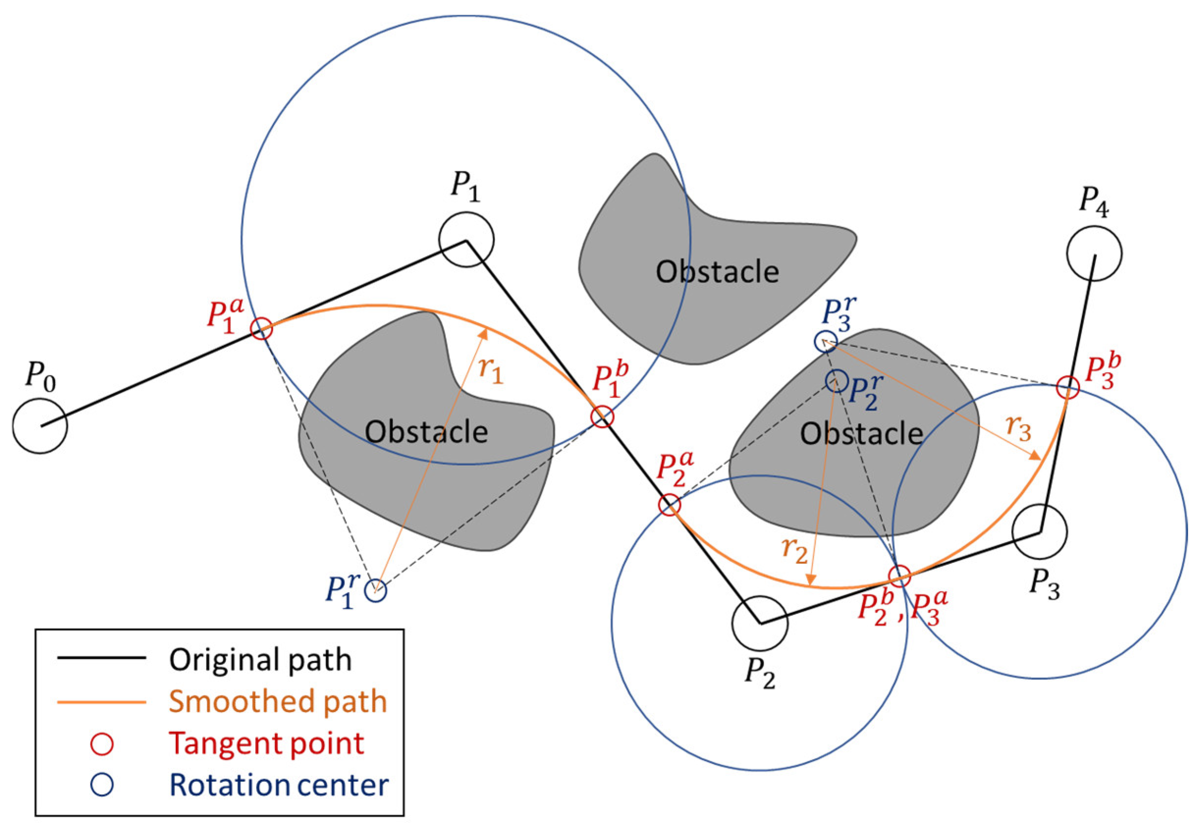
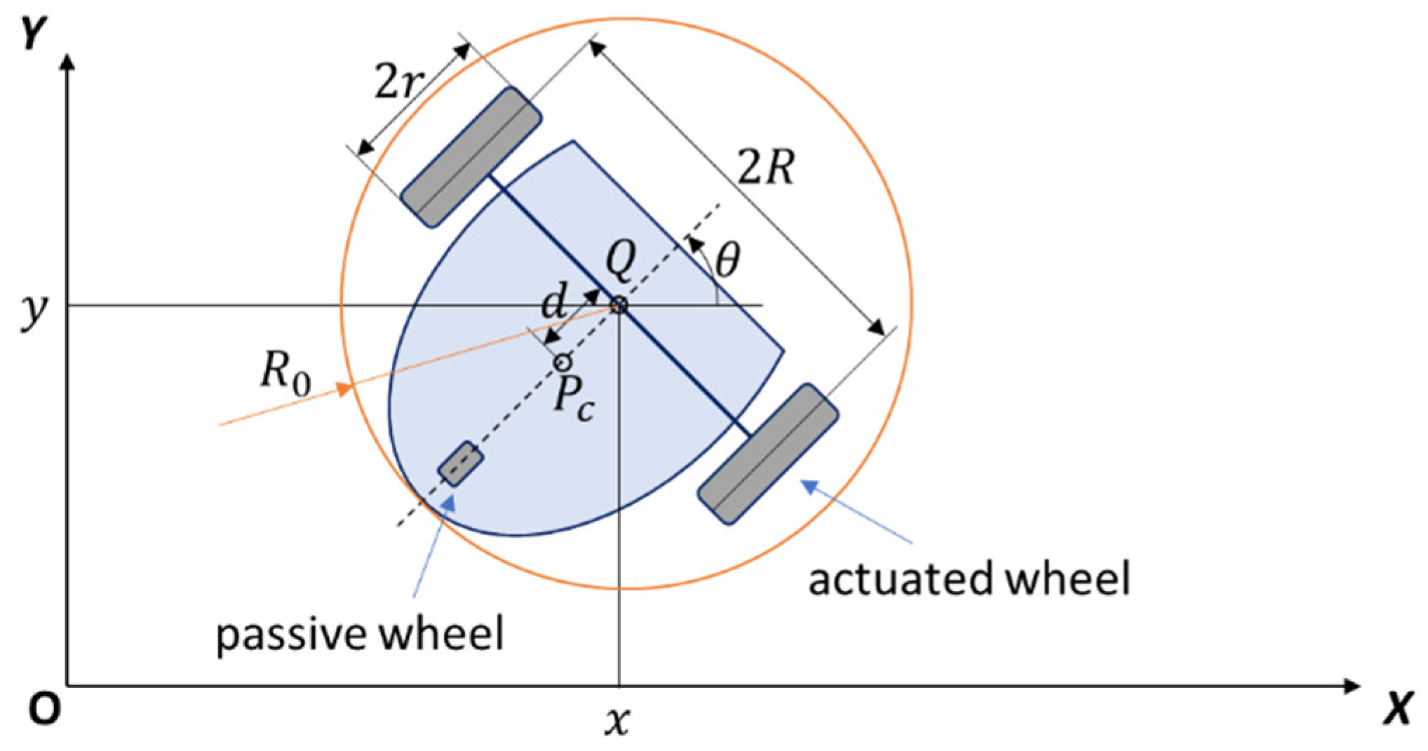
The purpose of path smoothing is to find an arc to replace the path around the path points so that the continuity of the orientation is obtained. Figure 2 shows an example of path smoothing on a five-point path. In this example, we have three arcs to replace part of the original path. For each point of path except the first and the last, its rotation radius, rotation center, and two tangent points are represented as r_i, $P_i^r$, $P_i^a$, and $P_i^b$, respectively. The relations between these points are given in (18).

$$\begin{array}{l}\left[\begin{array}{l}{x}_i^a\\ y_i^a\end{array}\right]=\left[\begin{array}{l}{x}_i-r_i\sin \left(\left|\Delta {\theta }_i\right|/2\right)\cos \left({\theta }_i\right)\\ x_i-r_i\sin \left(\left|\Delta {\theta }_i\right|/2\right)\sin \left({\theta }_i\right)\end{array}\right]\\ \left[\begin{array}{l}{x}_i^b\\ y_i^b\end{array}\right]=\left[\begin{array}{l}{x}_i+r_i\sin \left(\left|\Delta {\theta }_i\right|/2\right)\cos \left({\theta }_{i+1}\right)\\ x_i+r_i\sin \left(\left|\Delta {\theta }_i\right|/2\right)\sin \left({\theta }_{i+1}\right)\end{array}\right]\\ {\theta }_i{=\tan }^{-1}\left(\frac{y_i-y_{i-1}}{x_i-x_{i-1}}\right)+2m_i\pi ,\hspace{1em}{m}_i\in \mathbb{Z},s.t.0\le {\theta }_i<2\pi \\ \Delta {\theta }_i={\theta }_i-{\theta }_{i-1}+2n_i\pi ,\hspace{1em}{n}_i\in \mathbb{Z},s.t.-\pi \le {\theta }_i<\pi \end{array}$$

(18)

With a larger rotation radius, robots may move with less angular velocity to obtain higher linear velocity. Therefore, path smoothing becomes an optimization problem, and the fitness function is designed in (19) to maximum the rotation radius. c is a positive constant satisfying c > 1 to maintain log(r_i + c) > 0.

$$\underset{r_i\in (0,r_{\max }]}{\max }{\displaystyle {\sum }_{i=1}^{n-1}\log \left(r_i+c\right)}$$

(19)

The conditions of the optimization problem are given in (20).

$$\begin{array}{l}\overline{P_i{P}_i^b}+\overline{P_{i+1}{P}_{i+1}^a}\le \overline{P_i{P}_{i+1}},\hspace{1em}\forall i\in {\mathbb{Z}}^{+},i<n-2\\ \overline{P_1{P}_1^a}\le \overline{P_0{P}_1}\\ \overline{P_{n-2}{P}_{n-2}^b}\le \overline{P_{n-2}{P}_{n-1}}\\ State\left(B\left(Inde{x}_B\left(x,y\right)\right)\right)=free,\hspace{1em}\\ \hspace{1em}\forall P(x,y)\in \stackrel{⌢}{P_i^a{P}_i^b},\forall i\in {\mathbb{Z}}^{+},i<n-1\end{array}$$

(20)

3.3. Trapezoidal Velocity Profile

The trapezoidal velocity profile (TVP) is a simple and common method for motion planning by giving a fixed distance. In our case, the robot moves in a 2-D plane with two control inputs. Therefore, we consider implementing the trapezoidal velocity profile on both linear and angular velocities with the kinematic model of wheeled mobile robots in (21).

$$\dot{x}=v\cos \theta ,\dot{y}=v\sin \theta ,\dot{\theta }=\omega$$

(21)

Figure 3 shows an example of the trapezoidal velocity profile with (21) to replace an arc curve. Both linear and angular velocities are designed by TVP as (22) and shown in Figure 3b. The initial location of the robot is [x, y, θ] = [0, 0, 0]. In Figure 3a, an arc curve with same starting and ending point is added in to compare with the moving trajectory. The state of ending point in this example is [1.7100, 1.5934, 1.4997].

$$v=\{\begin{array}{ll}0\hfill & 0\le t<0.5\hfill \\ 2(t-0.5)\hfill & 0.5\le t<1\hfill \\ 1\hfill & 1\le t<3\hfill \\ 1-2(t-3)\hfill & 3\le t<3.5\hfill \\ 0\hfill & 3.5\le t<4\hfill \end{array},\hspace{1em}\omega =\{\begin{array}{ll}0.5t\hfill & 0\le t<1\hfill \\ 0.5\hfill & 1\le t<3\hfill \\ 0.5(3-t)\hfill & 3\le t<4\hfill \end{array}$$

(22)

Taking the example in Figure 2, three arc curves are replaced with the TVP method. Then, the linear velocities of three straight segments, which are P₀ to $P^a$₁, $P^b$₁ to $P^a$₂, and $P^b$₃ to P₄, are simply applied with traditional TVP, and their angular velocities are kept at zero. After combining three curves and three straight segments, the velocity profile from P₀ to P₄ is obtained, and the time function of this path can also be further obtained. Therefore, the time plan of this path is obtained.

The step-by-step process of the proposed path planning in this paper is given in Figure 4, including BRRT and three improving methods.

4. Controller Design and Stability Analysis

In this section, we develop a controller in four parts. The first part is at the kinematic level to determine the virtual reference velocities. The dynamic for controller design is included in the second part. In the second part, the controller law is also obtained to determine the control value with the virtual reference velocities. The mechanism of dynamic gain adjustment is shown in the third part to solve the saturation problem. Obstacle avoidance is shown in the last part.

4.1. Kinematic Controller

From the kinematic controller in (2), there are two parameters, r and R, in the system. For the convenience of parameter estimation, we define a₁ = 1/r, a₂ = R/r, and â_i is the estimation of a_i as i = 1, 2. The Lyapunov function V₁ is chosen as:

$$V_1=\frac{1}{2r}{x}_e^2+\frac{1}{2r}{y}_e^2+\frac{R}{r}{V}_{\theta }\left({\theta }_e\right)+\frac{1}{2{\gamma }_1}{\tilde{a}}_1^2+\frac{1}{2{\gamma }_2}{\tilde{a}}_2^2$$

(23)

where V_θ(θ_e) is a Lyapunov function of θ_e to V_θ > 0 as θ_e ≠ 2kπ and V_θ = 0 as θ_e = 2kπ with k ∈ ℤ. The estimation errors are defined as ã_i = a_i − â_i, i = 1, 2. γ₁ and γ₂ are positive constants, the gain of estimators. Using the error dynamic Equation (15), the time derivative of V₁ becomes:

$$\begin{array}{ll}{\dot{V}}_1=& x_e\left(-\frac{{\nu }_{wr}+{\nu }_{wl}}{2}+a_1{\nu }_r\cos {\theta }_e\right)+a_1{y}_e{\nu }_r\sin {\theta }_e\hfill \\ & +\frac{\partial V_e}{\partial {\theta }_e}\left(-\frac{{\nu }_{wr}-{\nu }_{wl}}{2}+a_2{\omega }_r\right)-{\displaystyle \sum _{i=1}^2\frac{{\tilde{a}}_i{\dot{\widehat{a}}}_i}{{\gamma }_i}}\hfill \end{array}$$

(24)

The virtual control law $\overline{z}={[{\overline{\nu }}_{wr},{\overline{\nu }}_{wl}]}^T$ is chosen as ${\overline{\nu }}_{wr}=h_1+h_2$ and ${\overline{\nu }}_{wl}=h_1-h_2$, where h₁ and h₂ are given in (25).

$$\begin{array}{l}{h}_1={\widehat{a}}_1{\nu }_r\cos {\theta }_e+k_x{x}_e\\ h_2={\widehat{a}}_2{\omega }_r+{\widehat{a}}_1{k}_y{y}_e{\nu }_r{\Omega }_y+k_{\theta }{\Omega }_{\theta }\end{array}$$

(25)

Then, the time derivative of V₁ becomes:

$$\begin{array}{ll}{\dot{V}}_1=& -k_x{x}_e^2+a_1{y}_e{\nu }_r\left(\sin {\theta }_e-k_y\frac{\partial V_e}{\partial {\theta }_e}{\Omega }_y\right)-k_{\theta }{\Omega }_{\theta }\frac{\partial V_e}{\partial {\theta }_e}\hfill \\ & -{\gamma }_1^{-1}{\tilde{a}}_1\left({\dot{\widehat{a}}}_1+{\gamma }_1{x}_e{\nu }_r\cos {\theta }_e+{\gamma }_1{y}_e{\nu }_r\sin {\theta }_e\right)\hfill \\ & -{\gamma }_2^{-1}{\tilde{a}}_2\left({\dot{\widehat{a}}}_2+{\gamma }_2{k}_y^{-1}{\Omega }_y^{-1}{\omega }_r\sin {\theta }_e\right)+q_0\hfill \end{array}$$

(26)

with

$$\begin{array}{ll}{q}_0=& 0.5x_e\left(-{\nu }_{wr}-{\nu }_{wl}+{\overline{\nu }}_{wr}+{\overline{\nu }}_{wl}\right)\hfill \\ & +0.5\left(k_y^{-1}{\Omega }_y^{-1}\sin {\theta }_e\right)\left(-{\nu }_{wr}+{\nu }_{wl}+{\overline{\nu }}_{wr}-{\overline{\nu }}_{wl}\right)\hfill \end{array}$$

(27)

Ω_y and Ω_θ are chosen as:

$$\begin{array}{l}\sin {\theta }_e-k_y{\Omega }_y\frac{d{V}_1}{d{\theta }_e}=0\\ {\Omega }_{\theta }\frac{d{V}_1}{d{\theta }_e}\{\begin{array}{l}=0,\hspace{1em}{\theta }_e=2k\pi ,k\in Z\\ >0,\hspace{1em}\mathrm{elsewhere}\end{array}\end{array}$$

(28)

with â₁ and â₂ are updated by:

$$\begin{array}{c}{\dot{\widehat{a}}}_1=-{\gamma }_1\left(x_e{\nu }_r\cos {\theta }_e+{\gamma }_1{y}_e{\nu }_r\sin {\theta }_e\right)\hfill \\ {\dot{\widehat{a}}}_2=-{\gamma }_2\left(k_y^{-1}{\Omega }_y^{-1}{\omega }_r\sin {\theta }_e\right)\hfill \end{array}$$

(29)

Then, V₁ becomes:

$${\dot{V}}_1=-k_x{x}_e^2-k_{\theta }{\Omega }_{\theta }\left(\partial V_e/\partial {\theta }_e\right)+q_0$$

(30)

q₀ comes from the error between virtual control law and the angular velocity of wheels, which should deal with the dynamic controller. For this reason, it can be ignored only considering the kinematic level, which gives that time derivative of V₁ ≤ 0.

4.2. Dynamic Controller

To simplify the complexity of the controller, the dynamic surface control is introduced though a first-order equation as:

$${\tau }_{\nu }{\dot{z}}_f+z_f=\overline{z},\hspace{1em}{z}_f\left(0\right)=\overline{z}\left(0\right),\hspace{1em}{\tau }_{\nu }>0$$

(31)

The velocity error is defined as:

$$z_e=z-z_f$$

(32)

Its time derivative is given as:

$$\begin{array}{cc}{\dot{z}}_e& =\dot{z}-{\dot{z}}_f=M^{-1}\left(R_a^{-1}N{K}_{T}u-\left(C\left(\dot{q}\right)+D+P_1\right)z-{\tau }_d\right)-{\dot{z}}_f\\ & \le {\left(M{R}_a\right)}^{-1}N{K}_T\left(u+\Phi W\right)\hfill \end{array}$$

(33)

In (33), the vector of system parameter W can be estimated by â₃ with the update law in (24), such that a₃ = W^TW. Φ is a based matrix of system variable. Both W and Φ are shown in (34).

$$\begin{array}{c}W={\left[\begin{array}{cccccccccc}\frac{r_{ar}{r}^3}{4R^2{n}_r{k}_{tr}}& \frac{r_{al}{r}^3}{4R^2{n}_l{k}_{tl}}& \frac{r_{ar}{d}_{11}}{n_r{k}_{tr}}+n_r{k}_{er}& \frac{r_{al}{d}_{22}}{n_l{k}_{tl}}+n_l{k}_{el}& \frac{r_{ar}{m}_{11}}{n_r{k}_{tr}}& \frac{r_{ar}{m}_{12}}{n_r{k}_{tr}}& \frac{r_{al}{m}_{12}}{n_l{k}_{tl}}& \frac{r_{al}{m}_{11}}{n_l{k}_{tl}}& \frac{r_{ar}{d}_{m1}}{n_r{k}_{tr}}& \frac{r_{al}{d}_{m2}}{n_l{k}_{tl}}\end{array}\right]}^T\hfill \\ \Phi =\left[\begin{array}{cccccccccc}-{\nu }_{wf}\left({\nu }_{wr}-{\nu }_{wf}\right)& 0& -{\nu }_{wr}& 0& -{\dot{z}}_{f1}& {\dot{z}}_{f2}& 0& 0& 1& 0\\ 0& {\nu }_{wr}\left({\nu }_{wr}-{\nu }_{wf}\right)& 0& {\nu }_{wf}& 0& 0& {\dot{z}}_{f2}& {\dot{z}}_{f1}& 0& 1\end{array}\right]\hfill \end{array}$$

(34)

Notice that ż_f1 and ż_f2 can be obtained easily with (31), and that is the reason why dynamic surface control can reduce the complexity of the controller. Then, the control law is chosen by:

$$u=-k_{\nu }{z}_e-0.5{\delta }_1^{-2}{\widehat{a}}_3\Phi {\Phi }^T{z}_e$$

(35)

The update law of â₃ is designed as:

$${\dot{\widehat{a}}}_3=0.5{\gamma }_3{\delta }_1^{-2}{z}_e^T\Phi {\Phi }^T{z}_e\hspace{1em}{\widehat{a}}_3\left(0\right)=0$$

(36)

Instead of estimating all the parameters in the dynamic equation, â₃ is the estimator of W^TW. Therefore, although this dynamic controller is simple, it can work without precise parameters.

4.3. Dynamic Gain Adjustment

To overcome the saturation problem, we adjust the gain of the controller by fuzzy logic control. As the conditions in (28) must be maintained, only k_x and k_θ are tuned. In this fuzzy logic control, the position error e and the duty of control value are the input, and the output tunes the ratio of gain r_k to achieve dynamic gain adjustment.

The major target is to reduce controller saturation. Therefore, we choose the larger one of u to define the duty of control value u₀ as (37).

$$u_0=\frac{\max \left(\left|u\right|\right)}{u_{\max }}$$

(37)

u_max is max driving voltage of the motors, so that 0 ≤ u₀ ≤ 1. The position error e is defined in (38).

$$e={\left(x_e^2+y_e^2+{\theta }_e^2\right)}^{1/2}$$

(38)

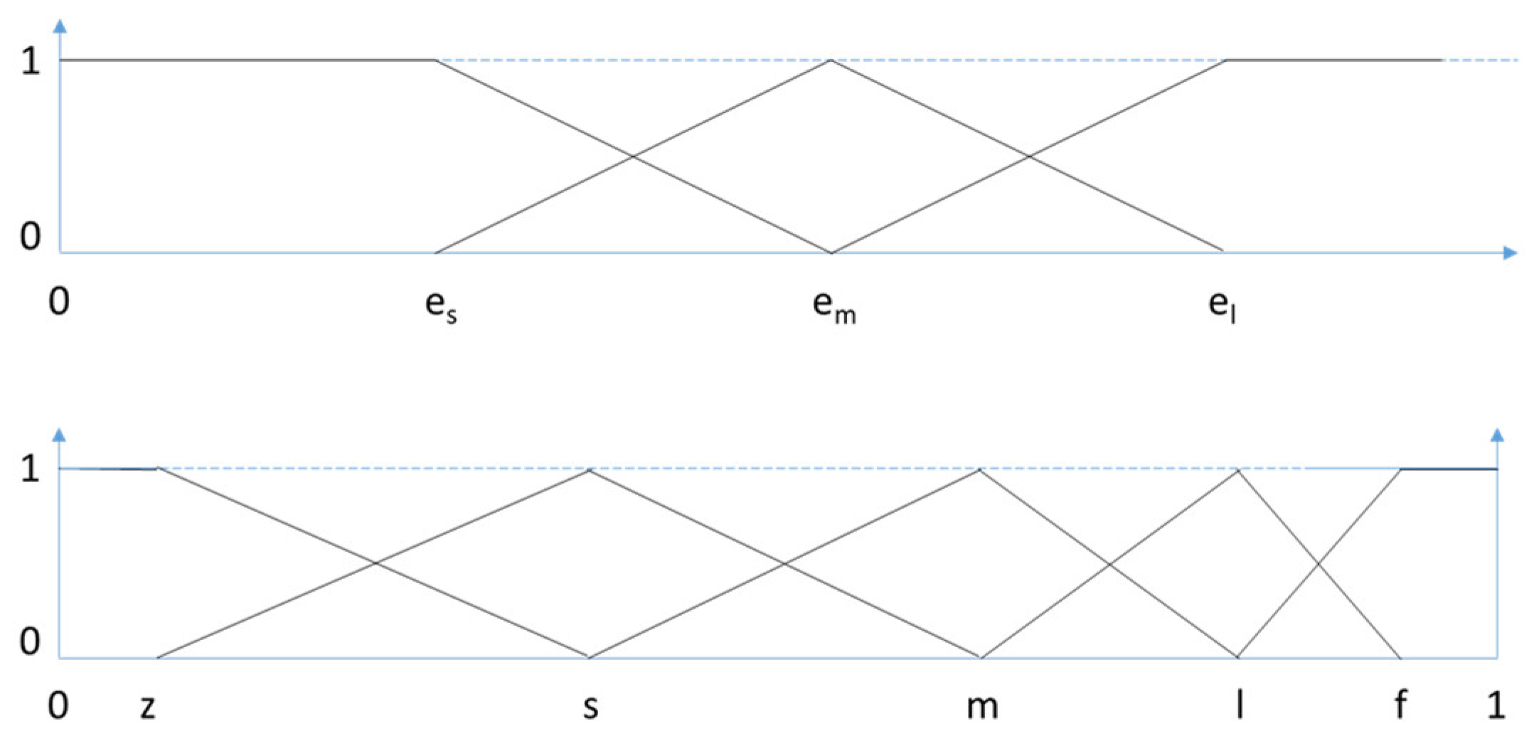
The membership function of the two inputs in shown in Figure 5. It is clear shown that the scale design of u₀ is asymmetric. This is because of the best duty of the motors should be put in the m scale to keep a good operating space.

Table 1. The role table of fuzzy logic control.

	u0	z	s	m	l	f
e
s		SR	NC	NC	NC	SI
m		SR	SR	NC	SI	SI
l		HR	SR	NC	SI	HI

is the rules to determine to increase or decrease the gain of the controller in each case. The output given in five levels in each case are: heavy increasing (HI), smooth increasing (SI), non-change (NC), smooth reducing (SR) and heavy reducing (HR).

Finally, the controller gain can be tuned as follows:

$$k_x^{*}=r_k{k}_x,\hspace{1em}{k}_{\theta }^{*}=r_k{k}_{\theta },\hspace{1em}{\dot{r}}_k=\mathrm{FLC}\left(u_0,e\right)$$

(39)

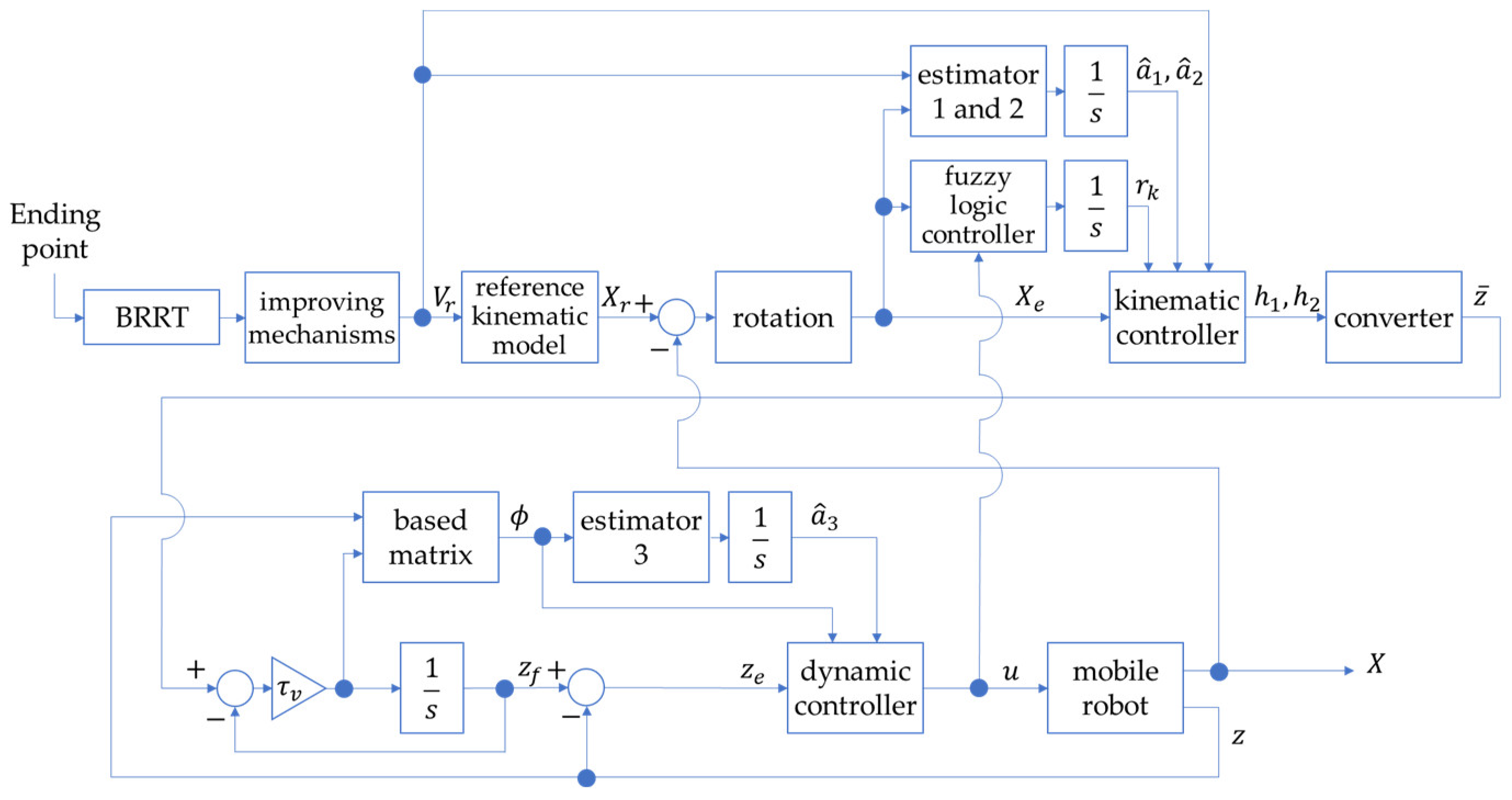
The structure diagram of proposed controller is shown on Figure 6. The reference velocity V_r of the virtual wheeled mobile robot and the path X_r based on the kinematic model are obtained from path planning algorithm. The tracking error X_e, obtained from (15) with a rotation is further provided to estimator 1 and 2 in (29) to obtain â₁ and â₂, provided to the fuzzy logic controller in (39) to obtain the gain ratio r_k, and provided to the kinematic controller in (25) with â₁, â₂, r_k, and a converter to obtain the virtual control law $\overline{z}$. The dynamic surface control proposes z_f from $\overline{z}$ with the first-order differential equation in (31). The based matrix Φ in (34) is provided to estimator 3 to obtain â₃ in (36). Finally, the dynamic controller for the mobile robot is designed in (35) with â₃, Φ, and z_e. The gain of the kinematic controller is also adjusted by u according to (37) and (39).

For traditional path planning algorithms, such as the A* algorithm and RRT algorithm in the grid, only the path X_r is provided, and its differentiability is not guaranteed. Hence, some controllers, such as PD, PID, and the proposed controller, are not suitable for direct application to traditional path planning algorithms. Take the PD controller as an example: the design of orientation control is given as the following:

$$u_b=k_p{\theta }_e+k_d{\dot{\theta }}_e$$

(40)

According to the definition of θ_e in (15), its time differential is obtained as ω_r − ω. Because the differentiability of X_r is not guaranteed, the angular velocity of the virtual wheeled mobile robot ω_r does not always exist. In this case, the time differential needs to be obtained by the numerical difference method from θ_e, which may cause approximation errors and the huge peak problem because of the discontinuity of orientation. However, ω_r is the second state of V_r in proposed path planning algorithm, so that ω_r always exists. Therefore, u_b has been fully defined, so that PD controller can be easily implemented in robot control with the proposed path planning algorithm.

4.4. Obstacle Avoidance

In this section, we focus on the ability of obstacle avoidance. The pseudo-code of obstacle avoidance is shown in Algorithm 4, where n is the number of levels. Figure 7 shows an example with four obstacles close to the original path with three obstacle avoidance levels. In this case, the obstacles are too close to the path and may cause collisions. Here, we define two parameters d₀ and d₁. d₀ is the hard-safe range so that the distance d between the obstacles and the robot should be larger than d₀. d₁ is the soft-safe range, which is also the threshold for obstacle avoidance design to take effect.

Algorithm4. Obstacle Avoidance

1: for i = 1 to length(Path) 2:     for j = 1 to n 3:         NewPath(i) = Path(i) 4:         for k = 1 to length(Obstacles) 5:             d = Distance(Path(i), Obstacles(k)) 6:             theta = Orientation(Obstacles(k), Path(i)) 7:             m = min(max(−(d − d1)/(d1 − d0), 0), 1) 8:             NewPath(i) = NewPath(i) + m * d1 * [cos(theta), sin(theta)] 9:         end 10:         Path = NewPath 11:     end 12: end 13: return NewPath

5. Experimental Results

The size of the map is 512 × 512 pixels and the origin is defined in the upper left corner of the map. Figure 8 shows the results of path planning. In Figure 8a, the start point is marked as a circle and located at (15, −30). The goal point is marked as a diamond and located at (270, −212). The blue polyline is the planned path by BRRT, and the red line is the tree of BRRT. Clearly, lots of unnecessary turns are included in the path. 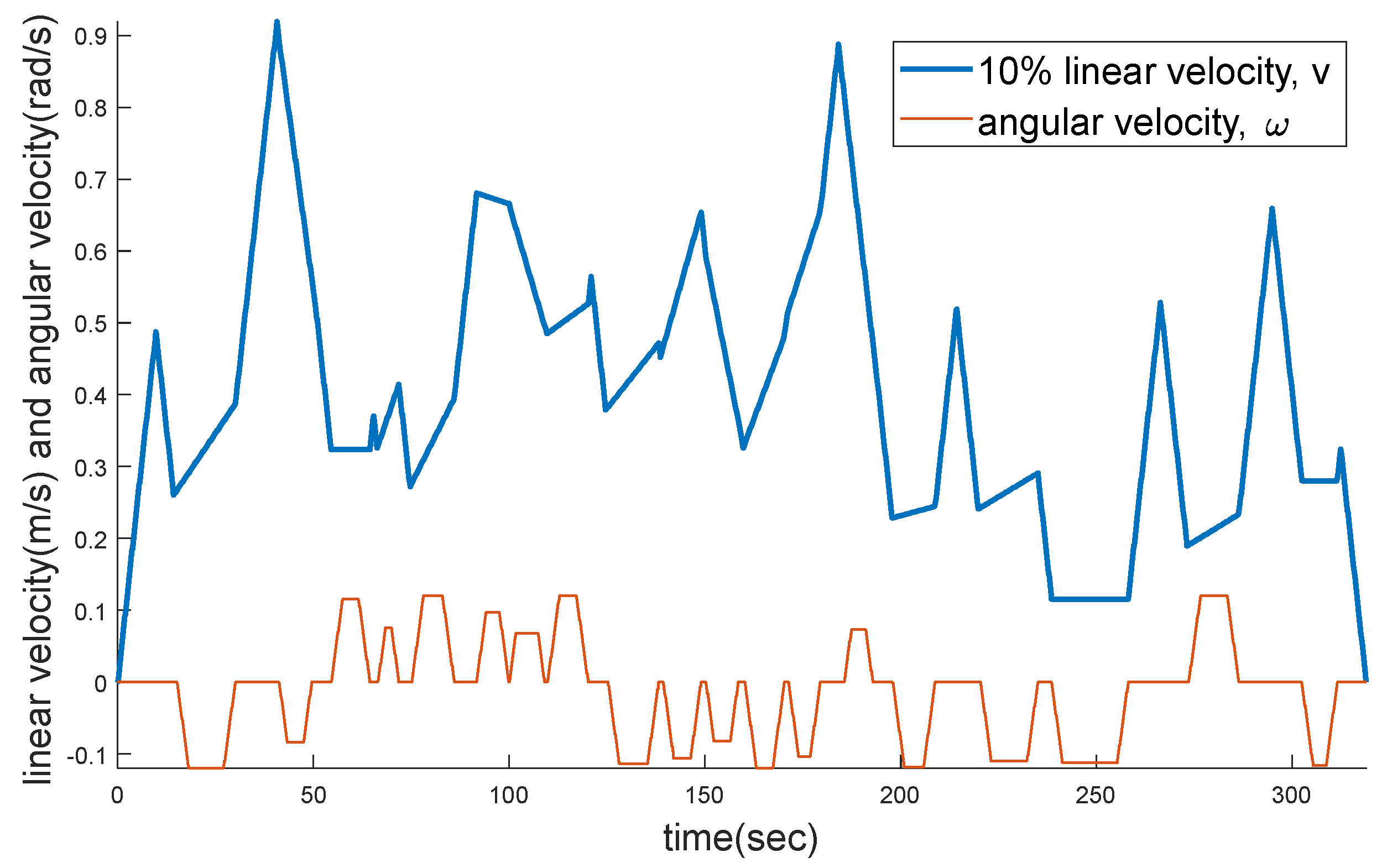Therefore, a smoothed path is given in Figure 8b, including the original path by BRRT, path pruning, and path smoothing. The minimum and maximum extension distance of BRRT is set between 3 to 10. The linear and angular velocities of the smoothed path are shown in Figure 9. The parameters of path smoothing are given in

Table 2. Parameters of path smoothing.

Name	Value	Name	Value
vmax	10 m/s	ωmax	0.12 rad/s
amax	0.5 m/s2	αmax	0.04 rad/s2
vratio	0.95	rmax	1000 m
h	0.01 s

.

In

Table 3. Performance of path pruning and path smoothing.

	Original Path		Pruned Path		Smoothed Path
	Length (m)	Num of Turns	Length (m)	Num of Turns	Length (m)	Num of Turns
average	1640.3	269.69	1357.8	22.210	1284.8	22.210
minimum	1550.0	245	1304.6	18	1258.5	18
maximum	1747.4	295	1430.5	26	1333.1	26
std. dev.	44.854	10.225	28.283	1.6955	16.707	1.6955

, a 100-times test is proposed to compare the paths in different stage, which are the original path, pruned path, and smoothed path. With the mechanism of path pruning, the average length is reduced from 1640.3 m to 1357.8 m, and the number of turns is reduced from 269.69 to 22.210. Data show that a lot of unnecessary turns are removed in path pruning. Although the mechanism of path smoothing does not change the number of turns required, the continuity of the path angle is improved, and the average length is further reduced to 1284.8 m.

The proposed controller is compared with P controller, which is a simple but widely used feedback control algorithm. The controller is designed as (41). Two errors, which are expected to be suppressed by the P controller, are defined as the position error e₀ and the orientation error e₁. The controller value u_b(0) and u_b(1) are designed proportional to the error e₀ and e₁, respectively. Both k_p0 and k_p1 are the positive gains of the P controller. Just like the design of ${\overline{\nu }}_{wr}=h_1+h_2$ and ${\overline{\nu }}_{wl}=h_1-h_2$, a converter is required to convert u_b to u in (40) according to the geometric relationship between the motor angle and the robot position.

$$\begin{array}{l}{e}_0={\left(x_e^2+y_e^2\right)}^{1/2},\hspace{1em}{e}_1={\theta }_e\\ u_b\left(0\right)=k_{p0}{e}_0,\hspace{1em}{u}_b\left(1\right)=k_{p1}{e}_1\\ u=\left[u_b\left(0\right)+u_b\left(1\right),u_b\left(0\right)-u_b\left(1\right)\right]\end{array}$$

(41)

The gains of the P controller are choosing as k_p0 = 6 and k_p1 = 8. The parameters of the robot and the gains of proposed controller are given in

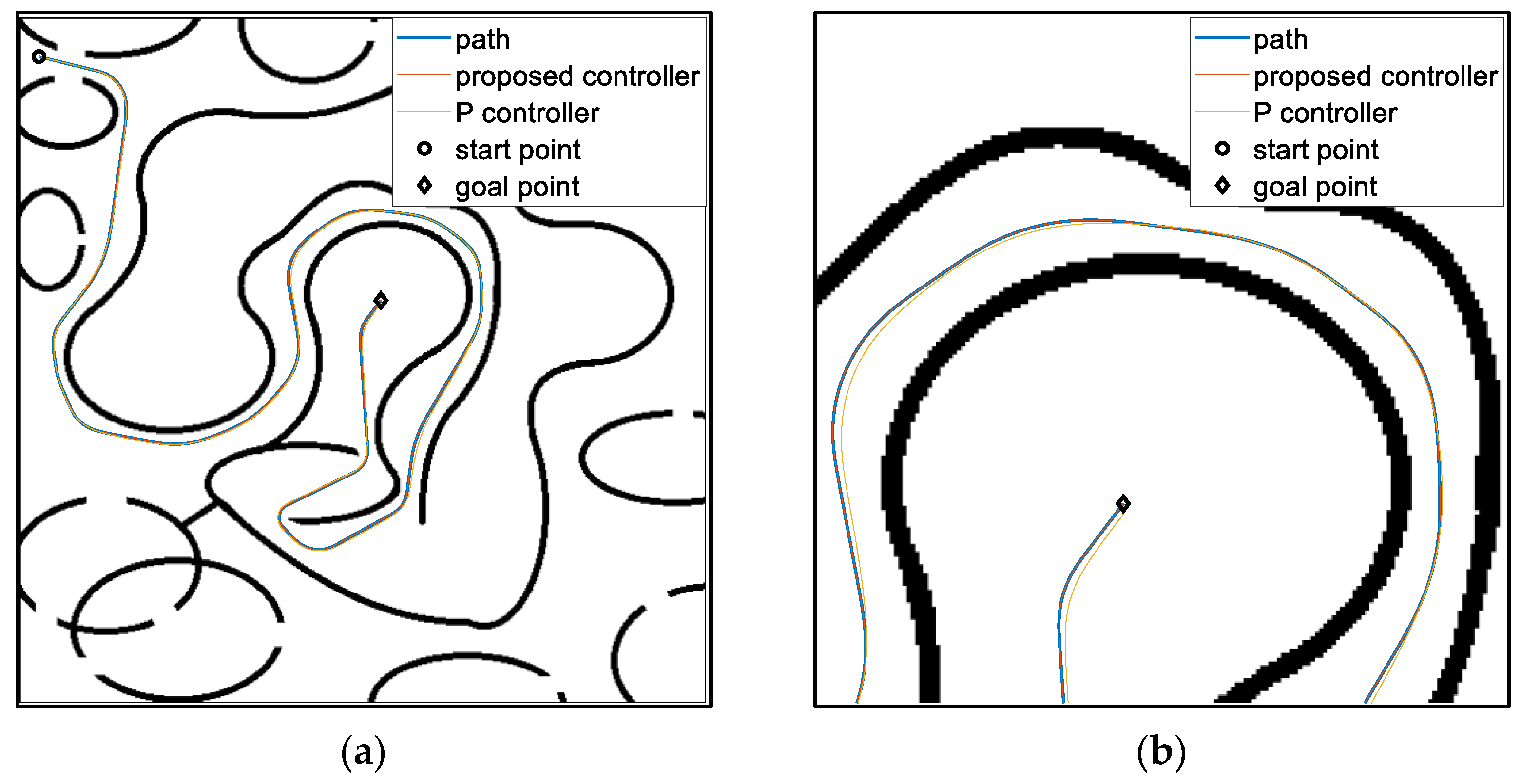
Table 4. The parameters of the robot and the gains of proposed controller.

Parameters
Name	Value	Name	Value
R	0.6 m	mw	0.7 kg
d	0.2 m	Ic	14.73 kgm2
r	0.1 m	Iw	0.004 kgm2
mc	25 kg	Im	0.002 kgm2
rar, ral	2.2 Ω	Ktr, ktl	0.281 oz-in/A
d11, d12	3 m	nar, nal	50
ker, kel	0.18 V/rad/s	umax	48 V
Gains
Name	Value	Name	Value
kx	3	γ1	30
ky	3	γ2	30
kθ	3	γ3	0.001
kv	4	δ1	10

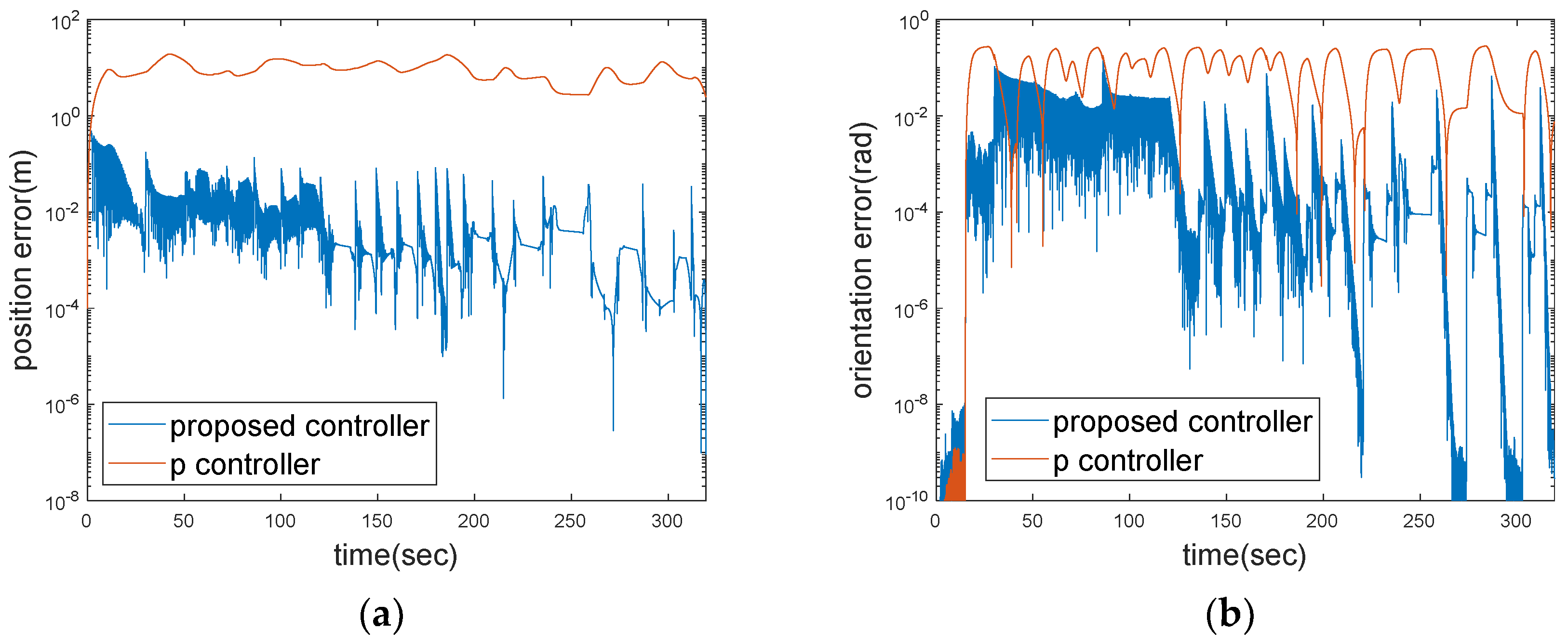
. The tracking results are shown in Figure 10, the tracking errors are shown in Figure 11, and the cumulative errors are shown in Figure 12. The tracking error is defined as e₀ in (40), and the orientation error is defined as the absolute value of e₁.

Table 5. Average tracking errors of P controller and proposed controller.

	P Controller		Proposed Controller
	Position Error (m)	Orientation Error (rad)	Position Error (m)	Orientation Error (rad)
average	8.9394	0.1159	0.0177	0.0070

shows the average tracking errors. The results show that the controller proposed in this paper outperforms the P controller in both position and orientation errors.

6. Conclusions

In this paper, we propose a navigation algorithm by using BRRT with several improvement measures to find the path with its time function, and by using an adaptive controller with dynamic gain adjustment in both the kinematics and dynamic models to reduce the tracking error and estimate the system parameters. A three-level obstacle avoidance algorithm is also proposed. In 100 simulations, this measure can save about 86% of the path planning time and 84% of the number of nodes. The robot’s movement time can also be reduced. The path planned in this way has the characteristics of velocity continuity, so it is suitable for application to control methods that require high order, especially in the design of controllers where the control term includes a differential term. Compared with P control, the proposed controller has better tracking ability to reduce the tracking errors in both position and orientation.