Abstract
Climate change is increasingly impacting both environments and human communities. Coastal regions in Thailand are experiencing more severe impacts, which vary based on the unique physical and socio-economic characteristics of each area. To assess the vulnerability of coastal regions in Thailand, this study focused on two provinces, Nakhon Si Thammarat (NST) and Krabi, each representing distinct coastal environments. NST, situated on the Gulf of Thailand’s east coast, has an agriculture-based economy, while Krabi, on the Andaman Sea’s west coast, relies heavily on tourism. The study utilized a multi-criteria decision analysis approach (MCDA) and GIS to analyze the Coastal Vulnerability Index at the sub-district level. The results revealed that, although NST was more vulnerable than Krabi to socio-economic factors such as the poverty rate and the number of fishery households, Krabi was much more vulnerable in the physical environment, including wave height, tidal level, coastal erosion, and slope. However, overall, Krabi exhibited high to the highest levels of coastal vulnerability, while NST displayed moderate to high levels. These findings provide valuable insights for policymakers and government agencies, aiding in the development of strategies to mitigate vulnerability and enhance the quality of life for local residents in both provinces.
1. Introduction
Low-lying coastal areas, situated between land and an ocean or lake, known as a coastline or shoreline, experience heightened vulnerability based on their physical exposure. This vulnerability is magnified if they are more susceptible to socio-economic factors (Alexandrakis et al. 2019; López-Dóriga and Jiménez 2020). Natural forces, such as sea level variations, wave activity, coastal and longshore currents, tidal fluctuations, vertical land movements, and sediment transport dynamics, exert significant influences on these coastal regions. Globally, coastal ecosystems have suffered due to a combination of factors, including eutrophication, overfishing, habitat degradation, and the impacts of climate change. Among the various challenges faced by coastal regions worldwide, one of the most severe is sea level rise (SLR). This phenomenon is expected to accelerate in the near future, with a projected global average increase of 60–90 cm above the current sea level by 2100. This rapid rise in sea levels is poised to result in more frequent and hazardous occurrences of flooding and erosion in coastal zones (Dolan and Walker 2006; IPCC 2022).
A range of other issues specific to coastal environments is further exacerbating the challenges associated with human utilization of coastal areas and posing threats to coastal ecosystems. These include problems such as marine pollution, marine litter, coastal development, tourism, and the loss of marine ecosystems. (Fairbanks 1989; Wahl et al. 2018; Langkulsen et al. 2022b). Additionally, the rate, type, and magnitude of climate change interact with the sensitivity and adaptive capacity of coastal systems. This interaction is expected to accelerate the speed of coastline retreat, rendering extensive coastal areas with high tourist value more vulnerable to disasters such as flooding and erosion (Dolan and Walker 2006). This process not only endangers the quality and value of services provided by coastal environments but also threatens the overall sustainability of coastal zones (Nicholls et al. 2007; Borchert et al. 2018; Wahl et al. 2018; Curoy et al. 2022). Hence, the intensification of any of the aforementioned processes, whether initiated by natural or human factors, has the potential to significantly degrade coastal areas, resulting in land loss, extensive damage to infrastructure, sea pollution, and a reduction in the biodiversity of marine resources (Neumann et al. 2015).
Vulnerability, in the context of disaster risk, refers to the extent of impact or damage caused by the combination of exposure, sensitivity, and adaptive capacity of individuals or communities in a specific area (Cardona et al. 2012). Coastal fragility, on the other hand, specifically pertains to the vulnerability of coastal regions and the people or communities residing in these coastal areas. To analyze the vulnerability of coastal areas worldwide, researchers have widely adopted and adapted the Coastal Vulnerability Index (CVI) approach, which considers various physical and socio-economic factors (Gornitz 1991; Markphol et al. 2021). The degree of impact or damage resulting from disasters varies depending on the unique physical and socio-economic characteristics of each area. While many factors used in vulnerability analysis are common across studies, variations may exist based on the study area’s size and data availability limitations (McLaughlin and Cooper 2010).
Physical factors commonly considered in vulnerability assessments include geomorphology, the extent of flooding affecting roads and buildings, wave height, tidal levels, sea level rise, and coastal erosion (McLaughlin and Cooper 2010; Duriyapong and Nakhapakorn 2011; Wies et al. 2016). Socio-economic factors contributing to vulnerability encompass aspects such as wealth, education, ethnicity, religion, gender, age, social class, disability, and health, which collectively characterize the local community (Cardona et al. 2012; Langkulsen et al. 2022a). Frequently used socio-economic factors in vulnerability analysis encompass the gender and age composition of the population, population density, education levels, income or poverty rates, access to healthcare systems, and internet accessibility (McLaughlin and Cooper 2010; Islam et al. 2015; Wies et al. 2016; Bevacqua et al. 2018; Apotsos 2019; Dintwa et al. 2019; Pricope et al. 2019).
A Geographic Information System (GIS) is a set of tools for handling spatial data, which proves valuable in helping analysts and decision-makers identify priorities based on various factors. GIS provides decision-makers with a flexible environment for researching and addressing complex geographical challenges (Seenath et al. 2016). Multi-Criteria Decision Analysis (MCDA) is a technique that can be used to combine stakeholder preferences and spatial information, converting them into quantitative values for assessment and subsequent decision-making. The Analytical Hierarchy Process (AHP) is a well-established pairwise comparison method within the realm of MCDA (Saaty 1988; Bera and Maiti 2021). The combination of GIS and MCDA allows for a rational assessment of the likely physical changes resulting from phenomena like flooding and erosion. However, it is worth noting that the subjectivity of expert opinions remains a challenge in this process. Nevertheless, this approach enables the preliminary planning of strategies for managing and safeguarding coastal resources and infrastructure in areas of interest (Seenath et al. 2016). In summary, the integration of GIS and MCDA serves the purpose of assisting decision-makers by providing them with the means to evaluate different options based on a range of sometimes conflicting criteria (Dhiman et al. 2018).
This study utilizes GIS-MCDA to assess the physical and socio-economic vulnerability to erosion and flooding in the Nakhon Si Thammarat (NST) and Krabi provinces. It considers significant physical factors shaping coastal geomorphology, including significant wave height, tidal level, sea level rise, slope, coastal erosion rate, household density, and land use type. Additionally, it incorporates relevant socio-economic factors such as the occupation of local residents, education level, unemployment, dependency ratio, and poverty rate into the analysis.
2. Materials and Methods
2.1. Research Framework
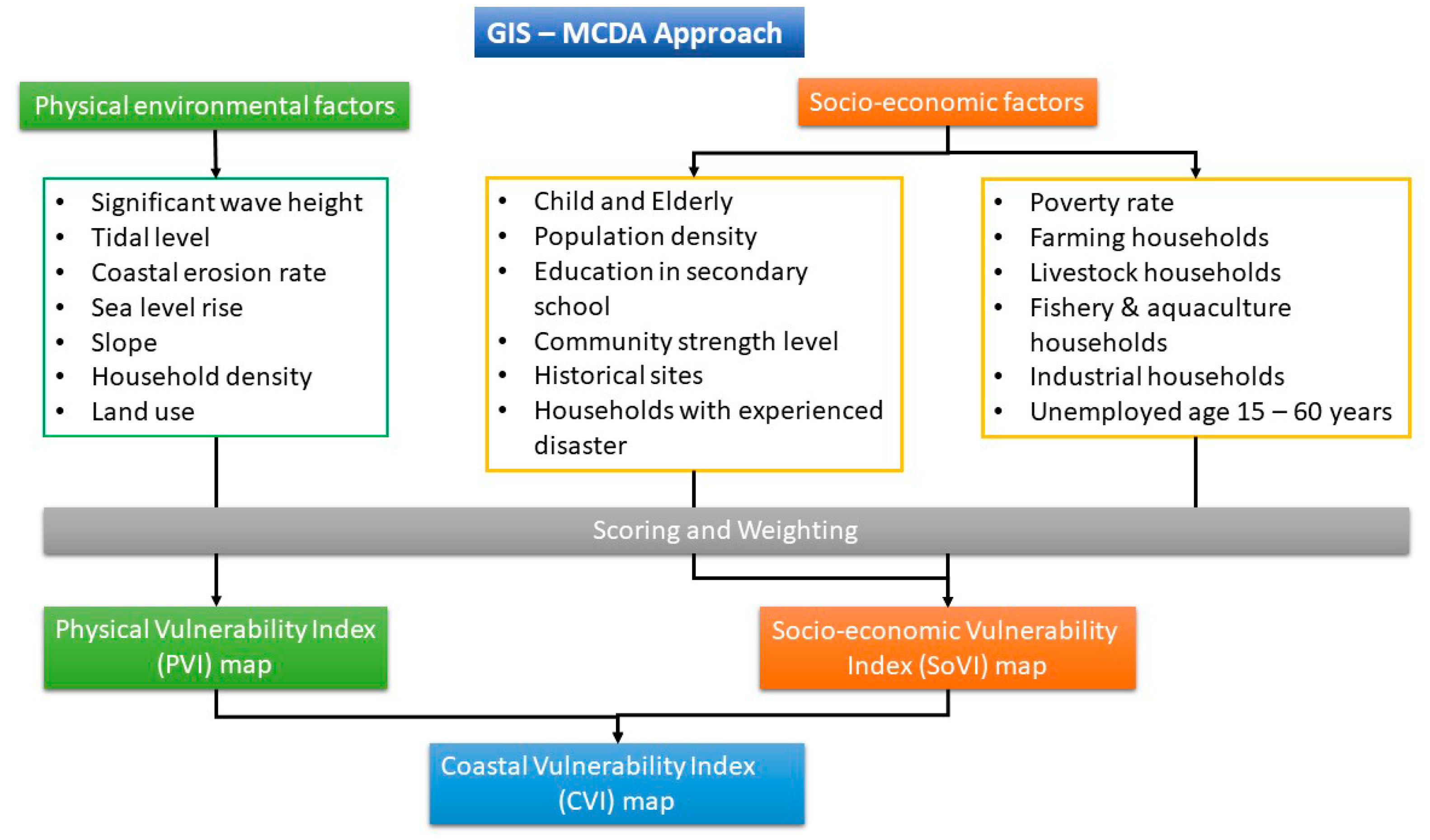
The GIS-MCDA approach research framework, as illustrated in Figure 1, utilized the Analytical Hierarchical Process (AHP), one of the Multi-Criteria Decision Analysis (MCDA) methods, in conjunction with Geographic Information System (GIS) technology to generate a Coastal Vulnerability Index map. The analysis commenced by assessing physical environment factors, leading to the creation of a Physical Vulnerability Index map (PVI map). Concurrently, social and economic factors were evaluated collectively to formulate a Socio-Economic Vulnerability Index map (SoVI map). Subsequently, the PVI and SoVI maps were integrated using a predetermined scoring and weighting methodology to generate the comprehensive CVI map.
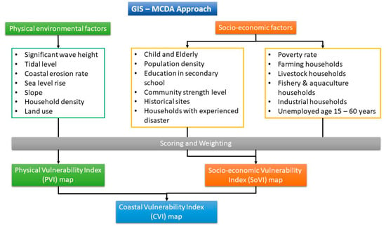
Figure 1.
Research framework.
2.2. Study Area and Datasets
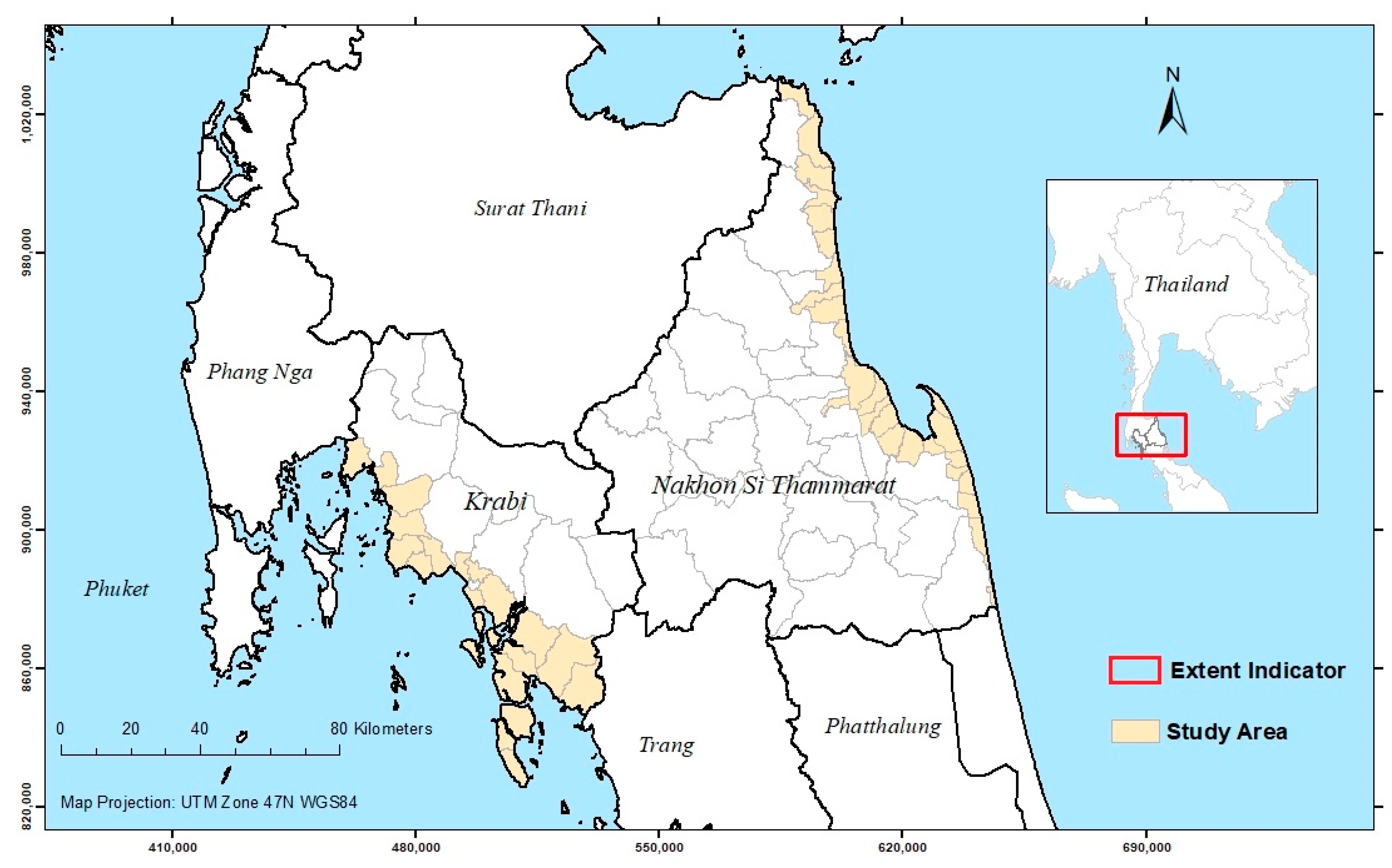
The study area encompasses 26 coastal sub-districts within 6 districts of NST and 20 coastal sub-districts within 5 districts of Krabi, situated in the southern region of Thailand, as depicted in Figure 2. NST is situated along the eastern coast, adjacent to the Gulf of Thailand, and its economy is primarily based on fisheries and aquaculture. The coastal stretch of NST spans approximately 225 km. In contrast, Krabi represents the western coast, adjacent to the Andaman Sea, and its economy relies heavily on tourism. The coastal line of Krabi extends for approximately 160 km. The spatial unit of analysis in both provinces is at the sub-district level. To analyze certain factors such as slope, house density, and land cover, it is necessary to use spatial units in the form of polygons. In the context of GIS data in Thailand, the smallest available administrative unit represented as polygons is the sub-district, while villages are depicted as points.
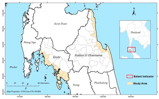
Figure 2.
Location of the study sub-districts.
The factors used in this study reflect the physical and socio-economic attributes of the study area that influence its vulnerability to natural processes such as storm impact, coastal erosion, and flooding. The physical and environmental data consist of 7 factors, which are detailed in Table 1. Additionally, socio-economic data, aggregated at the sub-district level, include 6 social factors and 6 economic factors, as outlined in Table 2.

Table 1.
Physical environmental factors used to measure PVI.
Table 2.
Socio-economic factors used to measure SoVI. All data are 2017.
2.2.1. Physical and Environmental Factors
Significant wave height: In NST, the prevailing wave directions are east and northeast, with the typical significant wave height falling within the 0.25–0.50 m range. Conversely, in Krabi, the primary wave directions are west and southwest, and the representative significant wave height predominantly falls within the 0.50–0.75 m range.
Tidal level: During the period from 1997 to 2007, the average high tide recorded at the Pak Phanang Station in NST was approximately +0.30 m. From 1981 to 2007, the Pak Nam Krabi Station in Krabi recorded an average peak tide of approximately +1.05 m. These average high tide values from the two stations were utilized as reference data for this study.
Sea Level Rise: The sea level rise data employed in this study were derived from a collaborative project conducted between Thailand and EC GEO2TECDI. This project aimed to investigate vertical land movement and sea level rise rates in the Gulf of Thailand and the Andaman Sea (Trisirisatayawong et al. 2011). According to the findings of this study, the rate of sea level rise in the Gulf of Thailand, specifically along the coast of NST, is approximately 4.5 mm/year. Conversely, along the Krabi coast, which borders the Andaman Sea, the rate of sea level rise is approximately 2.5 mm/year (Trisirisatayawong et al. 2011).
Slope: Digital Elevation Models (DEMs) were obtained from the Shuttle Radar Topography Mission (SRTM) DEM dataset featuring a spatial resolution of 90 m with a vertical accuracy of 10 m. These datasets were made available by the U.S. Geological Survey (USGS) and NASA. Subsequently, Geographic Information System (GIS) tools were employed to process these DEMs in order to derive slope data for the study area. Notably, the region in NST is characterized by a mountainous terrain oriented in a North–South direction, resulting in the formation of steep slopes in this area. In contrast, the topography of Krabi generally exhibits less pronounced slopes. To obtain representative slope values for each sub-district, the zonal statistics function in GIS was utilized to calculate the average pixel values within each sub-district.
Coastal erosion rate: Coastal erosion rate data for both NST and Krabi were obtained through an analysis conducted using the Digital Shoreline Analysis System (DSAS) in conjunction with Geographic Information System (GIS) tools (Curoy et al. 2022). The duration of this analysis spanned 30 years, during which the DSAS was employed to generate transects perpendicular to the shoreline baseline. Net Shoreline Movement (NSM) data were used to measure the net distance between the oldest recorded coastline and the most recent coastline within the study period. Subsequently, the NSM values were divided by 30, representing the number of years during which data were collected, in order to calculate erosion rates per year. It is noteworthy that several areas along the Krabi coastline exhibited higher erosion rates compared to those in NST. To determine the representative erosion rate for each sub-district, the GIS software (ArcGIS 10.7.1) utilized a zonal statistics function to compute the average value of pixels within the respective sub-district.
Household density: In 2019, data regarding household density was obtained from a statistical report on population and households published by the Office of Registration Administration, Department of Provincial Administration, Ministry of Interior. The number of households was utilized to calculate household density at the sub-district level, expressed as households per square kilometer (household/sq.km). Subsequently, the household density values were categorized into five classes for analysis. It should be noted that household density in Krabi was higher than in NST.
The number of households was further transformed into house density per square kilometer and classified into five vulnerability categories based on the house density range in the study area, as follows:
- Low vulnerability: Less than 250 houses per km2
- Moderate vulnerability: 250–500 houses per km2
- Medium vulnerability: 500–750 houses per km2.
- High vulnerability: 750–1000 houses per km2
- Very high vulnerability: More than 1000 houses per km2.
Land use type: In 2015, land use data was acquired from the Land Development Department, Ministry of Agriculture and Cooperatives. These data were categorized into five distinct land use categories, which include water bodies, grassland, forest, agriculture, and urban areas. Each of these land use types was assigned specific vulnerability levels, adapted from Duriyapong and Nakhapakorn (2011), representing their varying vulnerability to environmental risks and hazards.
2.2.2. Socio-Economic Factors
All the factors used in this study, except for those related to population and historical sites, were gathered by the Community Development Department (CDD) under the Ministry of Interior in the year 2017. It is worth noting that the CDD initially collected this data at the village level. However, for the purposes of this study, the data was aggregated and consolidated at the sub-district level.
Population data from the year 2017, which includes information on children and the elderly, as well as the total population count, was obtained from the Department of Provincial Administration (DOPA) website at the sub-district level. To assess the dependency ratio for each sub-district, the percentage of children and elderly individuals in relation to the total population was calculated. Additionally, the population density for each sub-district was calculated by dividing the total population of the sub-district by its land area in square kilometers.
Table 3 shows the statistical values of sub-districts for each factor. The percentage of farming households, livestock households, fishery and aquaculture households, and industrial households was calculated for comparison across those sub-districts. Subsequently, all values of these socio-economic factors were transformed into Z-scores, standardizing the data on a scale from 0 to 1, as previously explained, and then categorized into five vulnerability levels using equal interval classification.
Table 3.
The statistical values of socio-economic factors.
2.3. Vulnerability Level Scoring
In this study, the MCDA technique, combined with GIS, was utilized to assign scores to each factor based on their respective vulnerability levels. The vulnerability of each factor was then categorized into five classes, with a range from 5 (indicating the highest vulnerability) to 1 (representing the lowest vulnerability). The scoring of the physical environmental factors followed a prior study conducted in the Bangkok Metropolitan Region, as outlined by Duriyapong and Nakhapakorn (2011) (Table 4).
Table 4.
Physical and environmental factors, scoring scheme.
The socio-economic data layers, detailed in Table 3 with varied value ranges, were standardized into Z-scores using Equation (1). The resulting Z-scores comprised both positive and negative values, including some outliers. For the creation of five classes, Z-scores ranging from −2 to 2 were considered, with outliers less than −2 placed in the lowest class and outliers greater than 2 allocated to the highest class. Subsequently, in Table 5, the Z-scores were transformed into normalized scores spanning 0 to 1, and these normalized scores were further categorized into five classes using equal intervals. The class coded as 1 signifies the lowest vulnerability, while the class coded as 5 represents the highest vulnerability.
Table 5.
Normalized score in 5 categories of vulnerability.
- where Z = Z-Score
- x = a value of each factor
- mean = the mean value of each factor
- SD = the standard deviation of each factor
2.4. Coastal Vulnerability Index Map
2.4.1. Physical Vulnerability Index
To generate the Physical Vulnerability Index map, equal weights were assigned the physical environmental factors, following the approach of McLaughlin and Cooper (2010). The scores for each factors were aggregated, and the combined scores were then categorized into five classes using equal interval classification.
2.4.2. Socio-Economic Vulnerability Index
The weights for the socio-economic factors were determined through structured interviews, gathering insights from a selected group of seven participants representing both the public and private sectors in NST and Krabi. The participants were chosen from key stakeholders responsible for disaster management at the provincial level, including representatives from the Provincial Environmental section, Marine and Coastal Resources Department, Provincial Farmers Council, and Provincial Chamber of Commerce. The Analytical Hierarchical Process (AHP) technique, employed in previous research (Duriyapong and Nakhapakorn 2011; Cozannet et al. 2013; Bozorg-Haddad et al. 2021; Charuka et al. 2023), was used for this purpose. The participants conducted pairwise comparisons of factors, assigning important on a scale of 1–9 (as shown in Table 6) based on their perceived importance relative to one another. After the participants completed the assignment of importance levels, the weights of each factor were computed, and the Consistency Ratio (CR) was then calculated, as detailed in Bozorg-Haddad et al. (2021). Once the CR fell within an acceptable range (CR < 0.1), the average weights were used as the weights assigned to each socio-economic factor.
Table 6.
A pairwise comparison scale (Bozorg-Haddad et al. 2021).
2.4.3. Coastal Vulnerability Index
The coastal vulnerability score for each sub-district was calculated by combining the physical scores and the socio-economic weighted scores, with equal weighting. This total score was then used to create the coastal vulnerability index map through an equal-interval classification process.
3. Results
3.1. Physical Vulnerability Index
Significant Wave Height: Based on the information provided in Table 4, significant wave height along the NST coastline (ranging from 0.25 to 0.5 m) was classified as having a low vulnerability level. In contrast, along the Krabi coastline, where the significant wave height ranged from 0.50 to 0.75 m, it was classified as having a moderate vulnerability level.
Tidal Level: This study utilized the average high tide as the tidal level. According to the information presented in Table 4, the average high tide level along the NST coast, measured at +0.30 m, was classified as having a low vulnerability level. In contrast, along the Krabi coast, where the average high tide level was recorded at +1.05 m, it was classified as having a very high vulnerability level.
Sea Level Rise: According to Table 4, the rate of sea level rise along the NST coast was classified as having a high vulnerability level. On the other hand, the Andaman Sea along the Krabi coast was classified as having a low vulnerability level in terms of sea level rise.
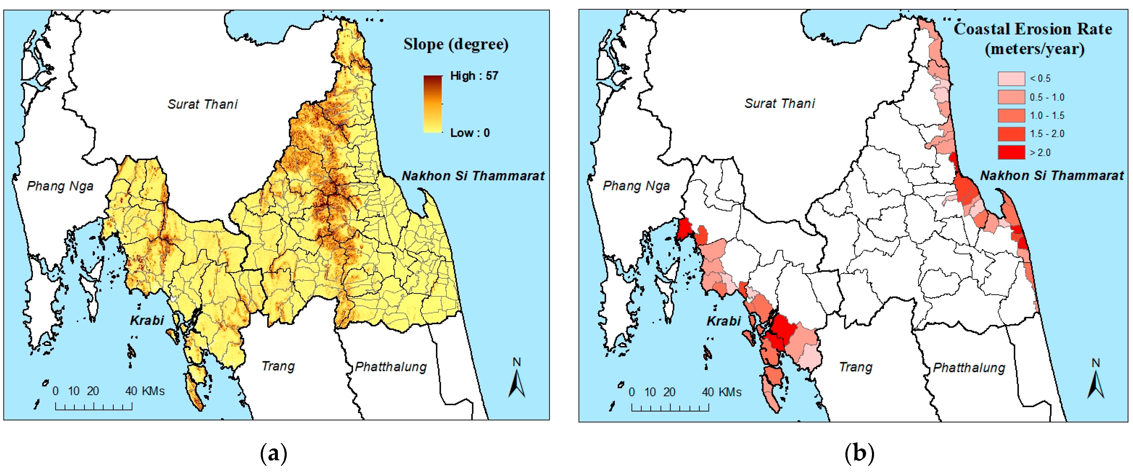
Slope: The slope data derived from the DEM is depicted in Figure 3a. Steep slopes are predominantly located in the mountainous regions further inland. These areas are not susceptible to coastal flooding but are more vulnerable to river flooding, particularly flash floods. Conversely, areas with a low slope, typically situated along the shoreline and coastal hinterland, are considered to have high vulnerability. They are prone to marine flooding caused by storm surges, increasing vulnerability during severe weather conditions.
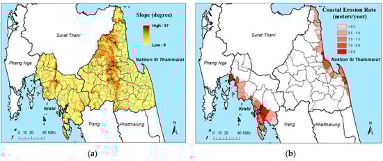
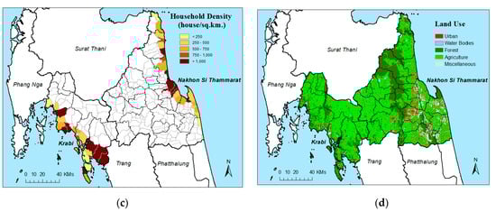
Figure 3.
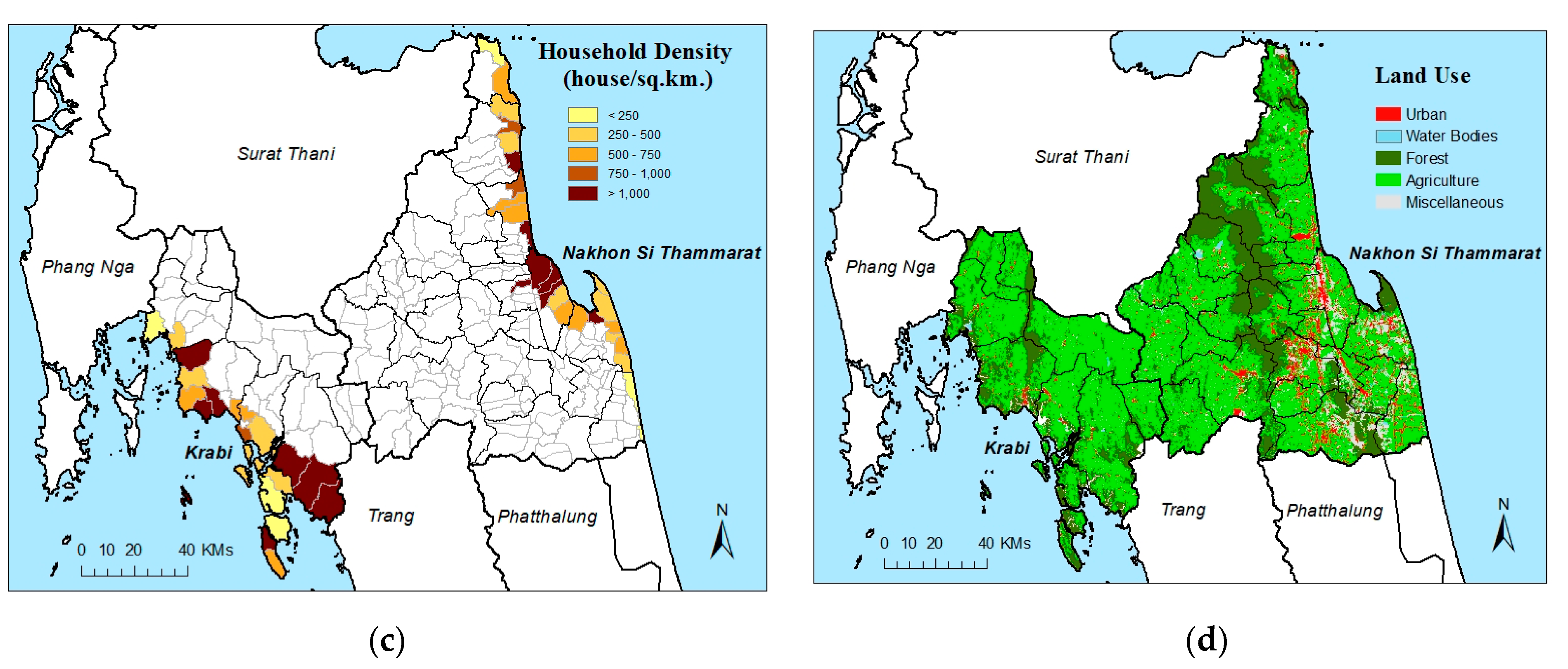
Physical and environmental factors used to generate the physical vulnerability index map: (a) Slope derived from DEM; (b) Coastal erosion; (c) Household density at sub-district level in 2019; (d) Land use in the study area in 2015.
Coastal Erosion Rate: The average erosion rate for each sub-district is illustrated in Figure 3b. Sub-districts with erosion rates exceeding 2 m per year were categorized as having the highest vulnerability. Conversely, sub-districts with erosion rates less than 0.5 m per year were deemed to have the lowest vulnerability.
Household Density: The household density in the study area varies, ranging from fewer than 250 houses per square kilometer to more than 1000 houses per square kilometer, as depicted in Figure 3c. The majority of sub-districts in NST have a density of less than 1000 houses per square kilometer. In contrast, most of the sub-districts in Krabi exhibit a density of more than 1000 houses per square kilometer.
Land Use Type: The study classified land use types based on the adapted criteria from the work of Duriyapong and Nakhapakorn (2011), as presented in Table 4. These criteria ranked urban areas as the most vulnerable, followed by agriculture areas, forested regions, grasslands, and water bodies as the least vulnerable. The study area primarily consists of agricultural areas, as depicted in Figure 3d. Urban areas, shown in red, occupy a larger area in NST compared to Krabi.
The Physical Vulnerability Index map in Figure 4 shows that the coastal regions in NST have lower vulnerability compared to Krabi. This difference arises from multiple factors contributing to lower vulnerability scores in NST, including reduced wave height, lower tides, decreased coastal erosion rates, lower household density, and predominant agricultural land use. In contrast, Krabi’s coastal areas, with higher household density and a greater proportion of urban land use, exhibit higher vulnerability levels.
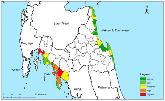
Figure 4.
Physical vulnerability index map of Nakhon Si Thammarat and Krabi.
3.2. Socio-Economic Vulnerability Index
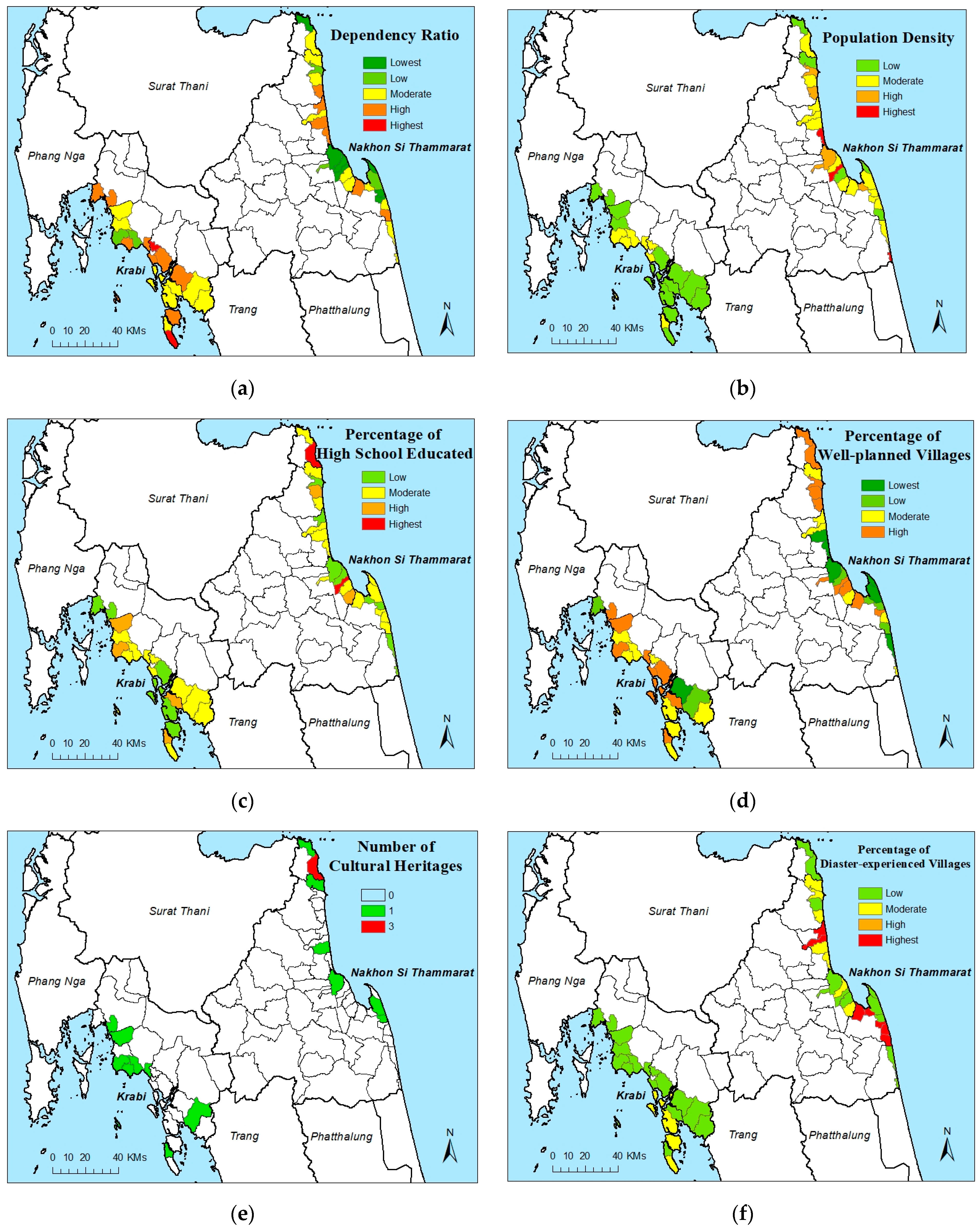
Figure 5 and Figure 6 depict the vulnerability levels of socio-economic factors. Notably, in NST, sub-districts showed higher vulnerability levels than Krabi in several socio-economic aspects, including dependency ratio, population density, villages with a history of natural disasters, poverty rates, number of farming households, and number of fishery households. However, the distribution patterns of the remaining factors appear more varied and do not consistently favor one province over the other.

Figure 5.
Social factors for generating a socio-economic vulnerability index map: (a) Dependency Ratio (percentage of children and old aged per total population); (b) population density; (c) percentage of high school educated (high percentage, low vulnerability in the key); (d) percentage of well-planned villages (high percentage, low vulnerability in the key); (e) number of the cultural heritages in sub-districts; (f) percentage of villages experienced natural disasters.
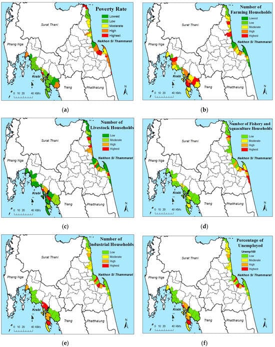
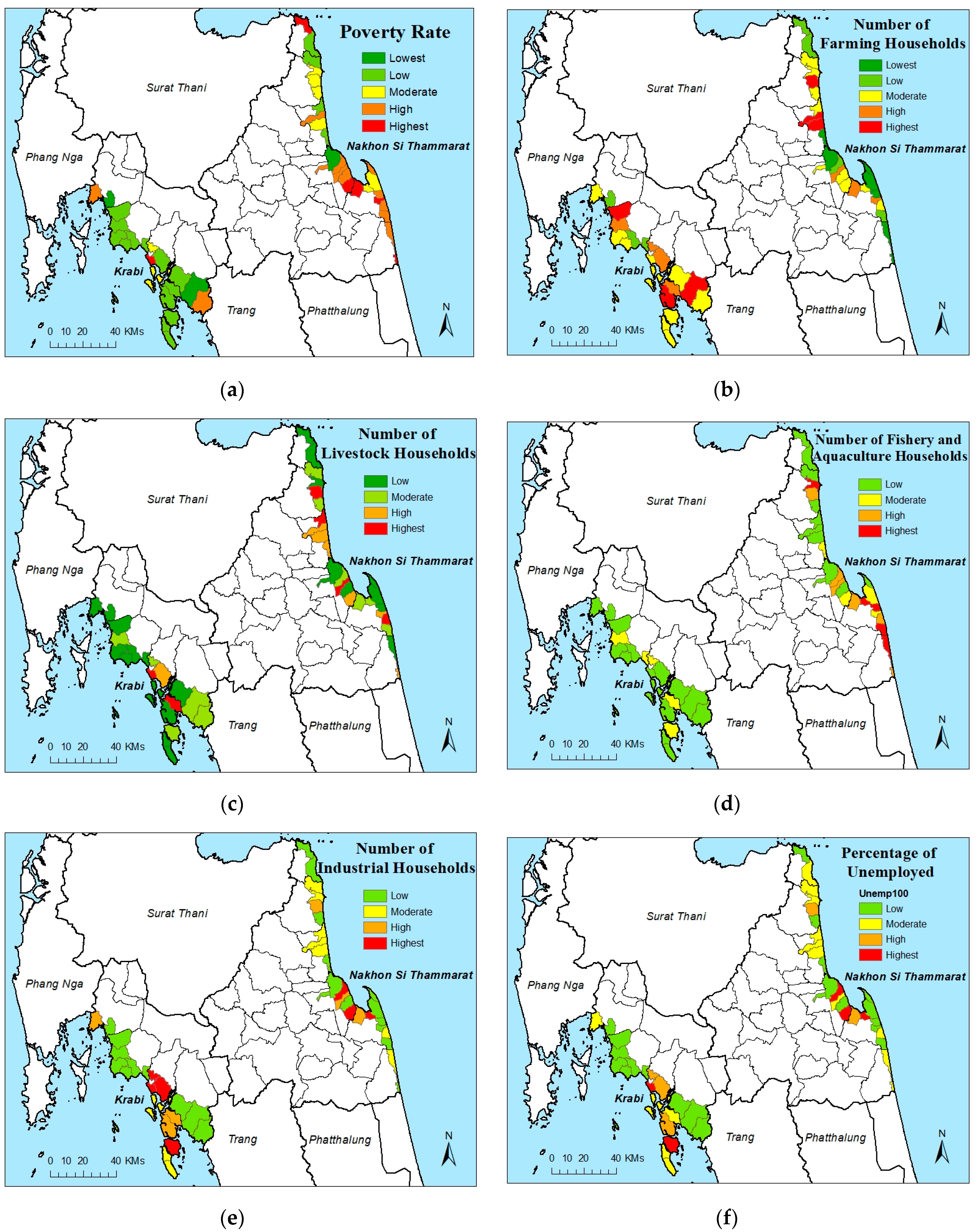
Figure 6.
Economic factors for generating a socio-economic vulnerability index map: (a) poverty rate (b) number of farming households; (c) number of livestock households; (d) number of fishery and aquaculture households; (e) number of small industrial households; (f) percentage of unemployed people.
The weights assigned to socio-economic factors, determined through the AHP analysis as explained in Section 2.4.2, are presented in Table 7. The factor related to fishery and aquaculture households was attributed the highest weight among the economic factors, emphasizing its significant importance in assessing vulnerability. On the other hand, among the social factors, the factor pertaining to households with prior experience of natural disasters received the highest weight, underscoring its critical role in evaluating vulnerability.
Table 7.
Weights of socio-economic factors given by participants.
For the socio-Economic Vulnerability Index map, the weighted scores of each sub-district for every socio-economic factor were computed by multiplying the coefficient by its respective score. Subsequently, these weighted scores were added to calculate the total socio-economic scores for each sub-district. A lower score indicates lower socio-economic vulnerability, while a higher score indicates higher socio-economic vulnerability.
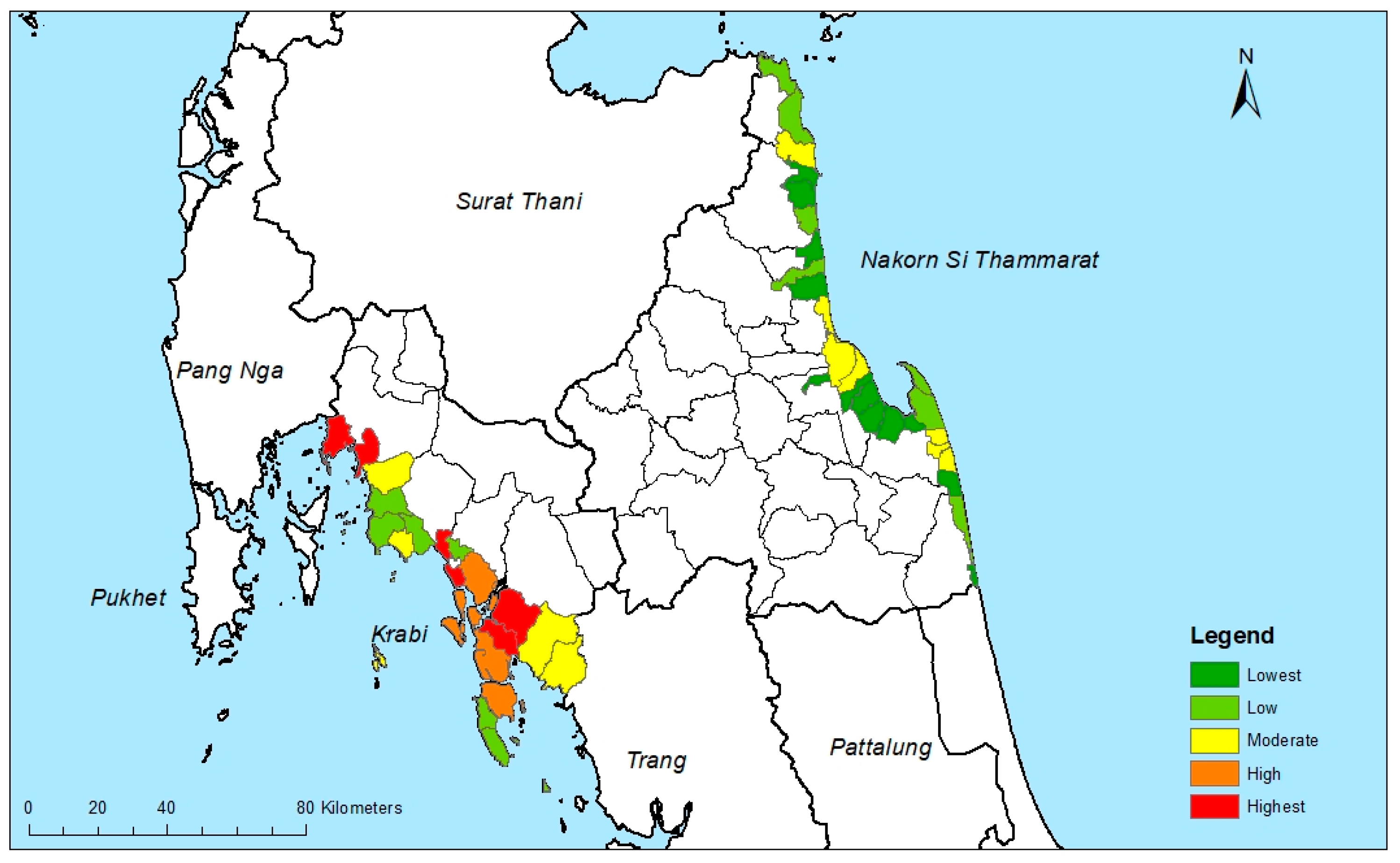
In Figure 7, it is evident that sub-districts along the coastlines of NST generally exhibited higher socio-economic vulnerability compared to those along the coastline of Krabi. Within Krabi Province, the southern coastal areas were more vulnerable than the northern coastal areas. Conversely, within NST, almost all sub-districts along the coast are classified as having high vulnerability, with the exception of the northern part of the province, which demonstrates lower vulnerability levels.
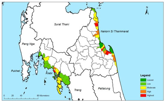
Figure 7.
Socio-economic vulnerability index map.
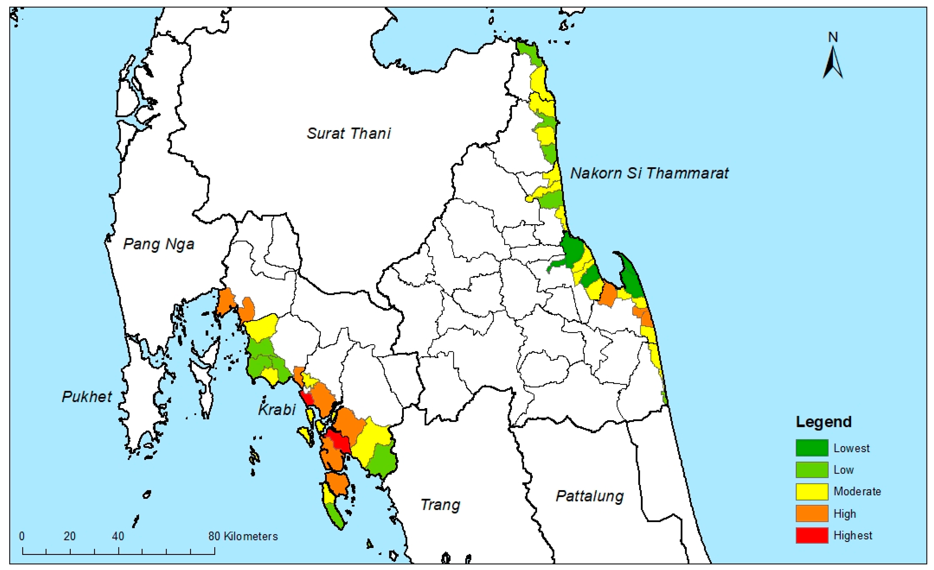
3.3. Coastal Vulnerability Index
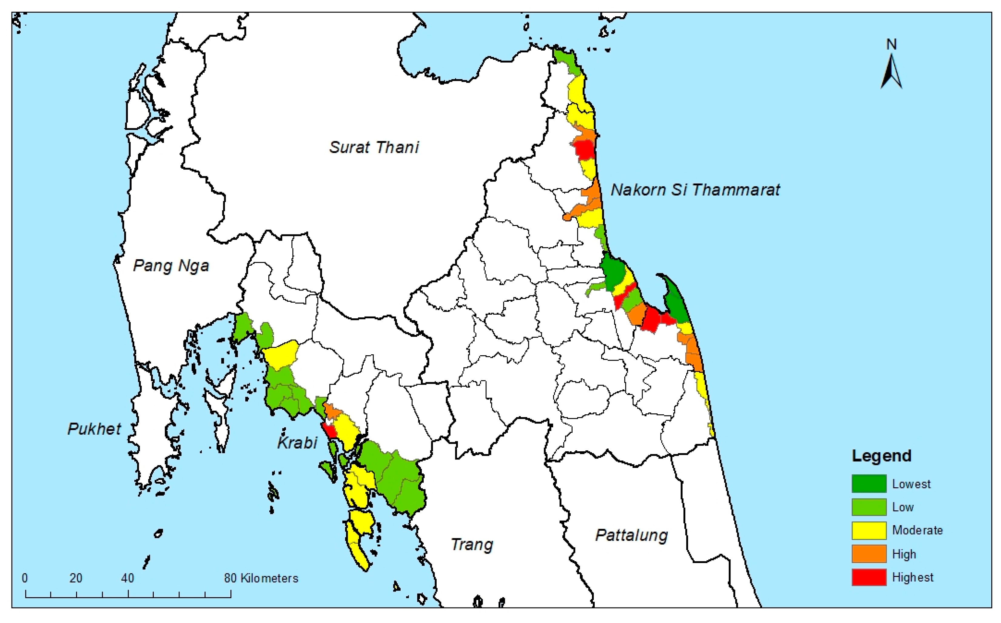
The CVI map resulting from the study is displayed in Figure 8. When comparing the vulnerability of the two provinces, it becomes apparent that the coastal areas of Krabi exhibit higher vulnerability than those of NST. This suggests that Krabi’s coastlines are more vulnerable to coastal erosion and flooding, while NST’s coastal areas are relatively less vulnerable.
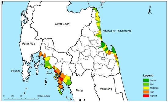
Figure 8.
Coastal vulnerability index map.
The six sub-districts with the highest level of vulnerability among the two provinces are as follows:
Krabi:
- Lamsak Sub-district in Ao Luk District;
- Taling Chan Sub-district in Nue Klong District;
- Huay Nam Khaw Sub-district in Klong Tom District;
- Klong Yang Sub-district and Ko Lunta Noi Sub-district in Ko Lanta District.
Nakhon Si Thammarat:
- Tja Sak in Mueang District
- Tha Phaya in Pak Phanang District
While most sub-districts in Krabi exhibit low to moderate levels of socio-economic vulnerability, the overall Coastal Vulnerability Index in Krabi is higher than that in NST. This heightened coastal vulnerability in Krabi is attributed to several physical environmental factors including higher significant wave height, higher tidal level, higher erosion rates, higher household density, and more urban areas.
4. Discussion
Previous studies have employed various approaches, or the same approach with different methods, to generate Coastal Vulnerability Index maps (Gornitz 1991; McLaughlin and Cooper 2010; Duriyapong and Nakhapakorn 2011; Kunte et al. 2014; Wies et al. 2016; Bevacqua et al. 2018; Apotsos 2019; Dintwa et al. 2019; Pricope et al. 2019; Alexandrakis et al. 2019; Charuka et al. 2023). This study was designed to utilize common variables from previous research, including coastal forcing, sea level rise, slope, population, education, employment, occupation, and poverty (McLaughlin and Cooper 2010; Duriyapong and Nakhapakorn 2011; Kunte et al. 2014; Wies et al. 2016; Bevacqua et al. 2018; Apotsos 2019; Dintwa et al. 2019; Pricope et al. 2019). The sub-district boundary was chosen as the smallest spatial extent of analysis due to data availability.
The findings of this study establish a significant foundation for informing and enhancing coastal management policies, particularly within the framework of Integrated Coastal Zone Management (ICZM). The generated PVI, SoVI, and CVI maps, along with insights from the Multi-Criteria Decision Analysis (MCDA) technique, provide valuable resources for policymakers aiming to address existing gaps in coastal management.
One notable contribution of this study is the identification of coping mechanisms for coastal erosion and flooding, as outlined by Langkulsen et al. (2022b). The risk mapping and database availability highlighted in their work align with the integrated tools developed in our study, serving as pivotal components for policy formulation and implementation. Similarly, Charuka et al. (2023) addressed the gap in the frequency and specificity of Coastal Vulnerability Index mapping over the past decade in Ghana by developing an updated CVI map. This recent CVI map is crucial for coastal planners, enabling the revision of short, medium, and long-term coastal adaptation policies with current and pertinent information.
The study’s maps serve as comprehensive tools that government agencies involved in coastal management can employ. The identification and categorization of vulnerability levels through PVI, SoVI, and CVI provide an understanding of socio-economic and environmental factors influencing vulnerability. Policymakers can use the vulnerability indices to develop targeted strategies for community resilience (Ariffin et al. 2023). Additionally, the study’s categorization into vulnerability classes facilitates the prioritization of areas requiring urgent attention and resource allocation.
The MCDA technique used in this study not only provided a systematic approach to weigh factors but also involved stakeholders in the decision-making process. Policymakers can adopt similar participatory approaches to ensure that decisions align with the needs and perspectives of local communities. This inclusivity fosters a sense of ownership among stakeholders and enhances the likelihood of successful policy implementation.
5. Conclusions
This study utilized the GIS-MCDA approach to calculate weighted scores for both physical and socio-economic factors, ultimately generating a Coastal Vulnerability Index map for NST and Krabi provinces. The results on the Coastal Vulnerability Index map reveal an uneven distribution of vulnerability among the sub-districts in the study area. Krabi’s sub-districts exhibit higher coastal vulnerability indices compared to those in NST, mainly due to their elevated physical vulnerability along Krabi’s coastlines. Although NST, on the whole, has higher socio-economic vulnerability than Krabi, the combined physical and socio-economic scores result in lower overall vulnerability scores for NST when compared to Krabi.
In summary, Krabi faces more substantial threats from physical factors, while NST’s vulnerabilities are mainly linked to socio-economic factors. The maps generated in this study, depicting various factors in both physical and socio-economic aspects, physical vulnerability index, socio-economic vulnerability index, and coastal vulnerability index, offer valuable insights for policymakers and government agencies. These insights can inform future management strategies aimed at reducing vulnerability and enhancing the quality of life for the local populations in both provinces.
The results of this study not only contribute valuable insights into coping mechanisms and vulnerability assessment but also present practical tools for policymakers. By integrating these findings into coastal management policies, policymakers can address gaps, foster community resilience, and work towards sustainable and effective ICZM practices.
Author Contributions
Conceptualization, P.C., U.L., K.N. and C.M.; methodology, P.C. and U.L.; validation, P.C.; formal analysis, P.C., V.L. and W.P.; investigation, P.C., C.C., S.B. and U.L.; writing—original draft preparation, P.C.; writing—review and editing, P.C., U.L., A.L. and C.M.; funding acquisition, K.N. and C.M. All authors have read and agreed to the published version of the manuscript.
Funding
This research was funded by the Economic & Social Research Council (ESRC), the Natural Environment Research Council (NERC), and the Thailand Social Research and Innovation (TSRI), grant number NE/S003231/1.
Institutional Review Board Statement
The study was conducted in accordance with the Declaration of Helsinki, and approved by the Institutional Ethics Committee of Mahidol University Central Institutional Review Board (MU-CIRB) (COA No. MU-CIRB 2019/020.3101).
Informed Consent Statement
Informed consent was obtained from all subjects involved in the study.
Data Availability Statement
The data presented in this study are available on request from the corresponding author. The data are not publicly available due to privacy issues. The data from the data source providers were permitted to use in this study only, cannot be disclosed to others.
Acknowledgments
The authors are grateful to experts for participating in the questionnaires survey contributing to the AHP process, and the data source providers for providing the valuable data for this study.
Conflicts of Interest
The authors declare no conflicts of interest.
References
- Alexandrakis, George, Sandro De Vita, and Mauro Di Vito. 2019. Preliminary risk assessment at Ustica based on indicators of natural and human processes. Annals of Geophysics 62: VO07. [Google Scholar] [CrossRef]
- Apotsos, Alex. 2019. Mapping relative social vulnerability in six mostly urban municipalities in South Africa. Applied Geography 105: 86–101. [Google Scholar] [CrossRef]
- Ariffin, Effi Helmy, Manoj Joseph Mathew, Adina Roslee, Aminah Ismailluddin, Lee Shin Yun, Aditya Bramana Putra, Ku Mohd Kalkausar Ku Yusof, Masha Menhat, Isfarita Ismail, Hafiz Aiman Shamsul, and et al. 2023. A multi-hazards coastal vulnerability index of the east coast of Peninsular Malaysia. International Journal of Disaster Risk Reduction 84: 103484. [Google Scholar] [CrossRef]
- Bera, Rakesh, and Ramkrishna Maiti. 2021. Multi hazards risk assessment of Indian Sundarbans using GIS based Analytic Hierarchy Process (AHP). Regional Studies in Marine Science 44: 101766. [Google Scholar] [CrossRef]
- Bevacqua, Anthony, Danlin Yu, and Yaojun Zhang. 2018. Coastal vulnerability: Evolving concepts in understanding vulnerable people and places. Environmental Science and Policy 82: 19–29. [Google Scholar] [CrossRef]
- Borchert, Sinead M., Michael J. Osland, Nicholas M. Enwright, and Kereen T. Griffith. 2018. Coastal wetland adaptation to sea level rise: Quantifying potential for landward migration and coastal squeeze. Journal of Applied Ecology 55: 2876–87. [Google Scholar] [CrossRef]
- Bozorg-Haddad, Omid, Hugo Loáiciga, and Babak Zolghadr-Asli. 2021. Analytic Hierarchy Process (AHP). In A Handbook on Multi-Attribute Decision-Making Methods. Edited by Omid Bozorg-Haddad, Hugo Loáiciga and Babak Zolghadr-Asli. Hoboken: Wiley. [Google Scholar] [CrossRef]
- Cardona, Omar-Dario, Maarten K. van Aalst, Jorn Birkmann, Maureen Fordham, Glenn McGregor, Rosa Perez, Roger S. Pulwarty, E. Lisa F. Schipper, and Bach Tan Sinh. 2012. Determinants of risk: Exposure and vulnerability. In Managing the Risks of Extreme Events and Disasters to Advance Climate Change Adaptation. Edited by Christopher B. Field, Vicente Barros, Thomas F. Stocker, Qin Dahe, David J. Dokken, Kristie L. Ebi, Michael D. Mastrandrea, Katharine J. Mach, Gian-Kasper Plattner, Simon K. Allen and et al. A Special Report of Working Groups I and II of the Intergovernmental Panel on Climate Change (IPCC). Cambridge and New York: Cambridge University Press, pp. 65–108. [Google Scholar]
- Charuka, Blessing, Donatus Bapentire Angnuureng, Emmanuel K. Brempong, Samuel K. M. Agblorti, and Kwesi Twum Antwi Agyakwa. 2023. Assessment of the integrated coastal vulnerability index of Ghana toward future coastal infrastructure investment plans. Ocean & Coastal Management 244: 106804. [Google Scholar] [CrossRef]
- Cozannet, Goneri Le, Manuel Garcin, T. Bulteau, C. Mirgon, M. L. Yates, M. Méndez, A. Baills, D. Idier, and C. Oliveros. 2013. An AHP-derived method for mapping the physical vulnerability of coastal areas at regional scales. Natural Hazards and Earth System Sciences 13: 1209–27. [Google Scholar] [CrossRef]
- Curoy, Jerome, Raymond D. Ward, John Barlow, Cherith Moses, and Kanchana Nakhapakorn. 2022. Coastal dynamism in Southern Thailand: An application of the CoastSat toolkit. PLoS ONE 17: e0272977. [Google Scholar] [CrossRef]
- Dhiman, Ravinder, Pradip Kalbar, and Arun B. Inamdar. 2018. GIS coupled multiple criteria decision making approach for classifying urban coastal areas in India. Habitat International 71: 125–34. [Google Scholar] [CrossRef]
- Dintwa, Kakanyo Fani, Gobopamang Letamo, and Kannan Navaneetham. 2019. Quantifying social vulnerability to natural hazards in Botswana: An application of cutter model. International Journal of Disaster Risk Reduction 37: 101189. [Google Scholar] [CrossRef]
- Dolan, A. H., and I. J. Walker. 2006. Understanding vulnerability of coastal communities to climate change related risks. Journal of Coastal Research SI 39: 1316–23. Available online: http://www.jstor.org/stable/25742967 (accessed on 20 October 2023).
- Duriyapong, Farida, and Kanchana Nakhapakorn. 2011. Coastal Vulnerability Assessment: A case study of Samut Sakhon coastal zone. Songklanakarin Journal of Science and Technology 33: 469–76. [Google Scholar]
- Fairbanks, Richard G. 1989. A 17,000-year glacio-eustatic sea level record: Influence of glacial melting rates on the Younger Dryas event and deep-ocean circulation. Nature 342: 637–42. [Google Scholar] [CrossRef]
- Gornitz, Vivien. 1991. Global coastal hazards from future sea level rise. Palaeogeography, Palaeoclimatology, Palaeoecology 89: 379–98. [Google Scholar] [CrossRef]
- IPCC. 2022. Sea Level Rise and Implications for Low-Lying Islands, Coasts and Communities. In The Ocean and Cryosphere in a Changing Climate: Special Report of the Intergovernmental Panel on Climate Change. Cambridge: Cambridge University Press, pp. 321–446. [Google Scholar]
- Islam, Ashraful, S. M. Kamrul Hassan, Abu Naime, Shakhawat Hossian, Mostafizur Rahman, and Mehedi Hasan Peas. 2015. Assessment of Socio-Economic Resilience Against Coastal Disasters in Sandwip Island of Bangladesh. Bangladesh Journal of Science Research 28: 161–70. [Google Scholar] [CrossRef]
- Kunte, Pravin D., Nitesh Jauhari, Utkarsh Mehrotra, Mahender Kotha, Andrew S. Hursthouse, and Alexandre S. Gagnon. 2014. Multi-hazards coastal vulnerability assessment of Goa, India, using geospatial techniques. Ocean & Coastal Management 95: 264–81. [Google Scholar] [CrossRef]
- Langkulsen, Uma, Desire Tarwireyi Rwodzi, Pannee Cheewinsiriwat, Kanchana Nakhapakorn, and Cherith Moses. 2022a. Socio-Economic Resilience to Floods in Coastal Areas of Thailand. International Journal of Environmental Research and Public Health 19: 7316. [Google Scholar] [CrossRef]
- Langkulsen, Uma, Pannee Cheewinsiriwat, Desire Tarwireyi Rwodzi, Augustine Lambonmung, Wanlee Poompongthai, Chalermpol Chamchan, Suparee Boonmanunt, Kanchana Nakhapakorn, and Cherith Moses. 2022b. Coastal Erosion and Flood Coping Mechanisms in Southern Thailand: A Qualitative Study. International Journal of Environmental Research and Public Health 19: 12326. [Google Scholar] [CrossRef]
- López-Dóriga, Uxía, and José A. Jiménez. 2020. Impact of Relative Sea-Level Rise on Low-Lying Coastal Areas of Catalonia, NW Mediterranean, Spain. Water 12: 3252. [Google Scholar] [CrossRef]
- Markphol, Adirake, Jawanit Kittitornkool, Derek Armitage, and Ponlachart Chotikarn. 2021. An integrative approach to planning for community-based adaptation to sea-level rise in Thailand. Ocean & Coastal Management 212: 105846. [Google Scholar] [CrossRef]
- McLaughlin, Suzanne, and J. Andrew G. Cooper. 2010. A multi-scale coastal vulnerability index: A tool for coastal managers? Environmental Hazards 9: 233–48. [Google Scholar] [CrossRef]
- Neumann, Barbara, Athanasios T. Vafeidis, Juliane Zimmermann, and Robert J. Nicholls. 2015. Future Coastal Population Growth and Exposure to Sea-Level Rise and Coastal Flooding—A Global Assessment. PLoS ONE 10: e0118571. [Google Scholar] [CrossRef] [PubMed]
- Nicholls, Robert J., Poh Poh Wong, Virginia Burkett, Jorge Codignotto, John Hay, Roger McLean, Sachooda Ragoonaden, and Colin D. Woodroffe. 2007. Coastal systems and low-lying areas. Climate Change 2007: Impacts, Adaptation and Vulnerability. In Contribution of Working Group II to the Fourth Assessment Report of the Intergovernmental Panel on Climate Change. Edited by Martin L. Parry, Osvaldo F. Canziani, Jean P. Palutikof, Paul van der Liden and Clair E. Hanson. Cambridge: Cambridge University Press, pp. 315–56. [Google Scholar]
- Pricope, Narcisa G., Joanne N. Halls, and Lauren M. Rosul. 2019. Modeling residential coastal flood vulnerability using finished-floor elevations and socio-economic characteristics. Journal of Environmental Management 237: 387–98. [Google Scholar] [CrossRef] [PubMed]
- Saaty, Thomas L. 1988. What is the analytic hierarchy process? In Mathematical Models for Decision Support. Heidelberg and Berlin: Springer, pp. 109–21. [Google Scholar]
- Seenath, Avidesh, Matthew Wilson, and Keith Miller. 2016. Hydrodynamic versus GIS modelling for coastal flood vulnerability assessment: Which is better for guiding coastal management? Ocean & Coastal Management 120: 99–109. [Google Scholar] [CrossRef]
- Trisirisatayawong, Itthi, Marc Naeije, Wim Simons, and Luciana Fenoglio-Marc. 2011. Sea level change in the Gulf of Thailand from GPS-corrected tide gauge data and multi-satellite altimetry. Global and Planetary Change 76: 137–51. [Google Scholar] [CrossRef]
- Wahl, Thomas, Sally Brown, Ivan D. Haigh, and Jan Even Øie Nilsen. 2018. Coastal Sea Levels, Impacts, and Adaptation. Journal of Marine Science and Engineering 6: 19. [Google Scholar] [CrossRef]
- Wies, Shawn W. Margles, Vera N. Agostini, Lynnette M. Roth, Ben Gilmer, Steven R. Schill, John English Knowles, and Ruth Blyther. 2016. Assessing vulnerability: An integrated approach for mapping adaptive capacity, sensitivity, and exposure. Climatic Change 136: 615–29. [Google Scholar] [CrossRef]
Disclaimer/Publisher’s Note: The statements, opinions and data contained in all publications are solely those of the individual author(s) and contributor(s) and not of MDPI and/or the editor(s). MDPI and/or the editor(s) disclaim responsibility for any injury to people or property resulting from any ideas, methods, instructions or products referred to in the content. |
© 2024 by the authors. Licensee MDPI, Basel, Switzerland. This article is an open access article distributed under the terms and conditions of the Creative Commons Attribution (CC BY) license (https://creativecommons.org/licenses/by/4.0/).