

The Role of Mechanical Ventilation in Indoor Air Quality in Schools: An Experimental Comprehensive Analysis
 , , , ,
  ,
,  and
and
Abstract
1. Introduction
- Zero energy: achieved through the installation of a photovoltaic system capable of covering all the annual electrical, thermal, and cooling needs of the classroom;
- Controlled physical (dust) and chemical (CO2 and VOC) contamination: ensured by the installation of a mechanical ventilation system;
- Controlled microbiological contamination: implemented through a protocol for sanitizing furniture and surfaces using probiotic microorganisms and eliminating chemical disinfectants, with a reduction in pathogenic microorganisms;
- Introduction of various types of plants and green walls;
- Optimization of the classroom’s interior design.
2. Materials and Methods
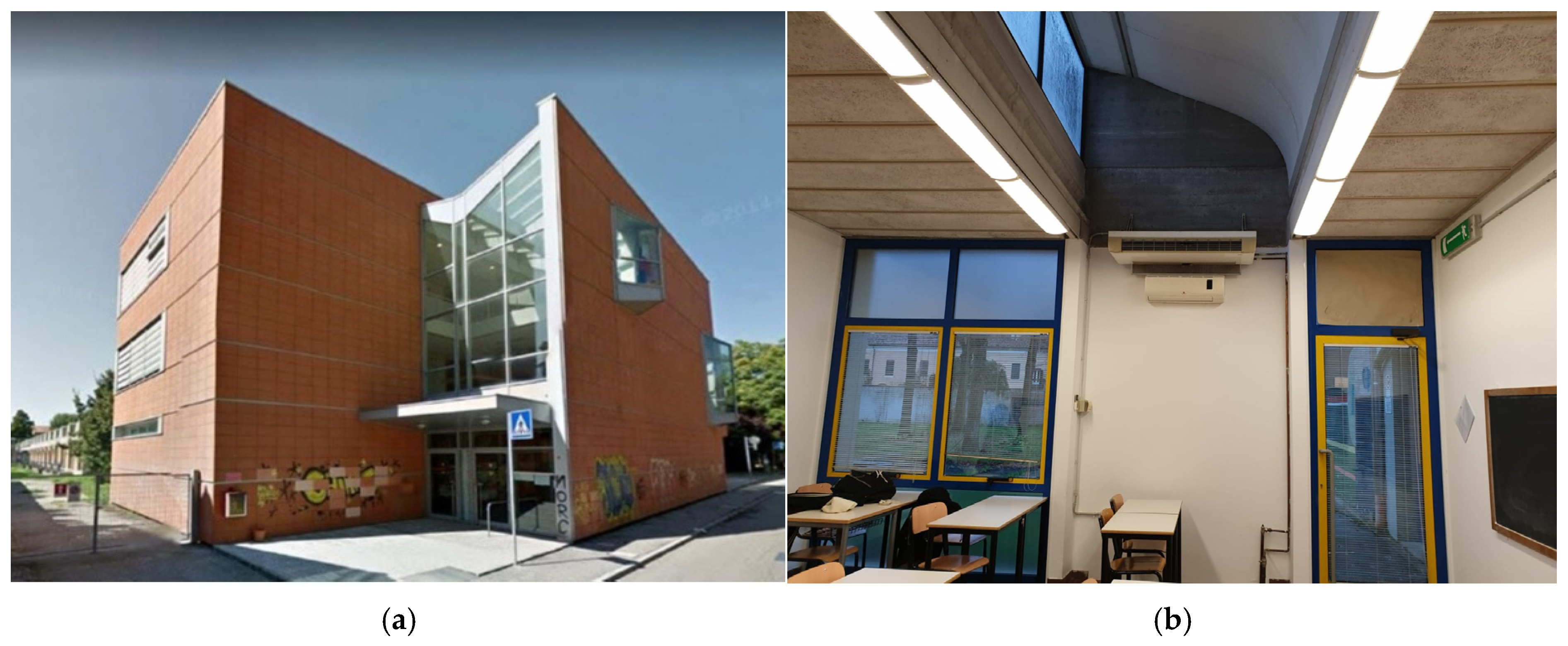
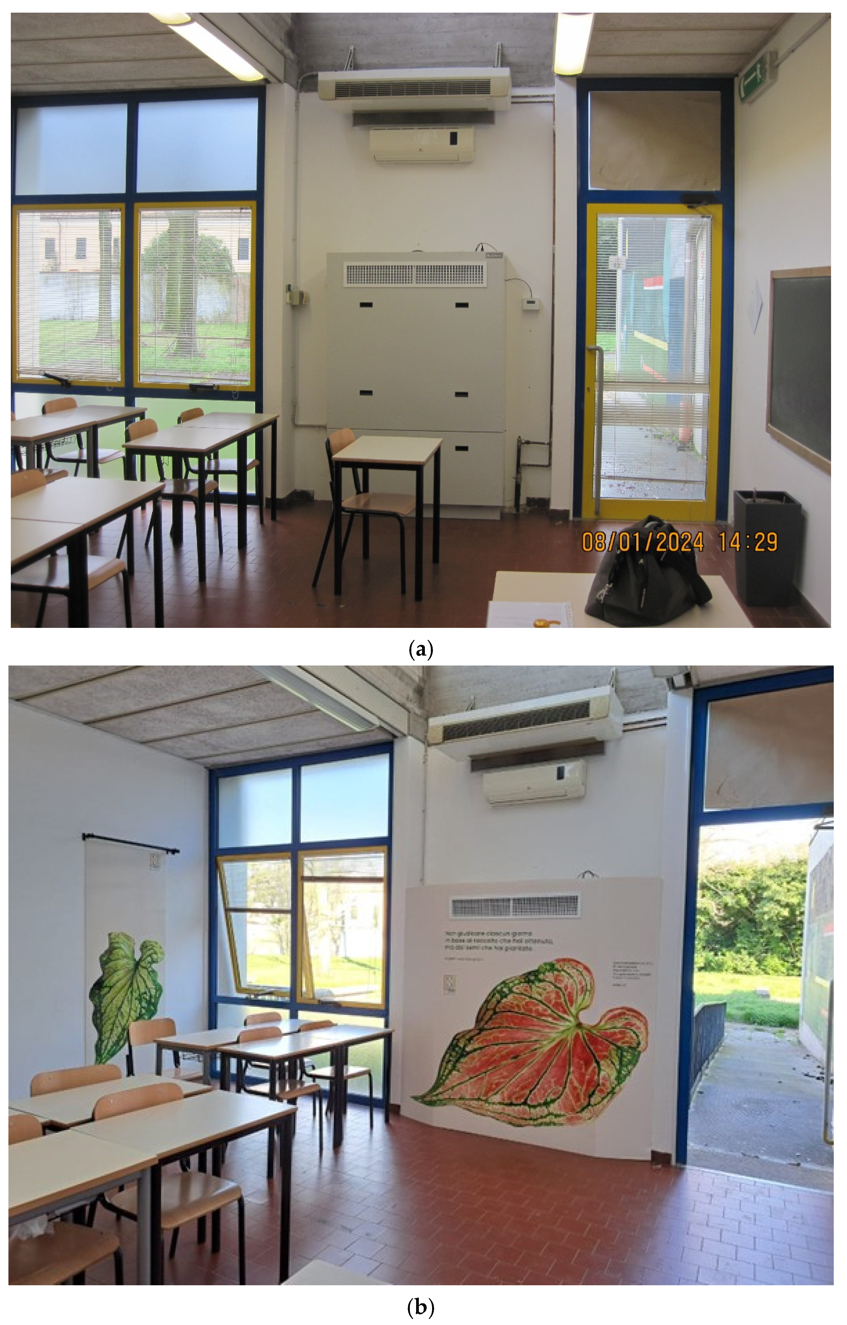
2.1. Building and Heating System Description
2.2. Controlled Mechanical Ventilation Unit
2.3. Set-Up of the Analysis and Sensors’ Position
- -
- The first phase (from mid-September 2023 to 31 December 2023) focused on using only natural ventilation in the classroom (Sensor 1 active);
- -
- The second phase (from 6 January 2024 onwards) involved mechanical ventilation (Sensor 1, Sensor 2, and MVHR active).
3. Results and Discussion
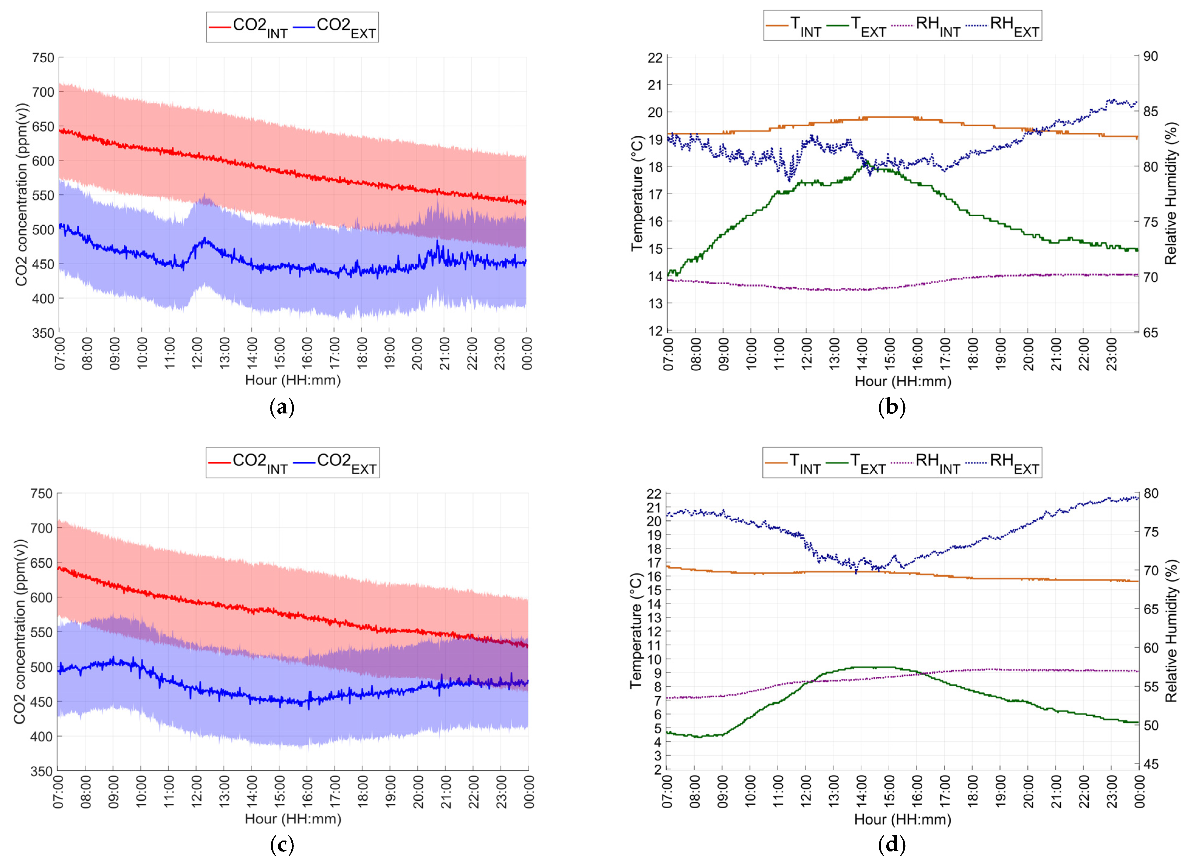
3.1. Thermohygrometric and CO2 Concentration Analysis (October 2023–April 2024)
3.2. CO2 Emission Rate per Person Inside the Classroom
- μCO2 and μair are the molar masses of CO2 and air, which are 44 g/mol and 29 g/mol, respectively;
- vmol,air is the molar volume of air, which depends on temperature. At 20 °C, it is 24.05 × 10⁻³ m3/mol;
- fCO2 is the molar (or volume) fraction expressed as a percentage, representing the ratio of nCO2/nair divided by 106. For example, at a concentration of 1000 ppm(v) in the environment, the volume fraction is 0.1%, as shown in Equation (4):
3.3. IAQ Analysis (February 2024–November 2024)
4. Conclusions
- -
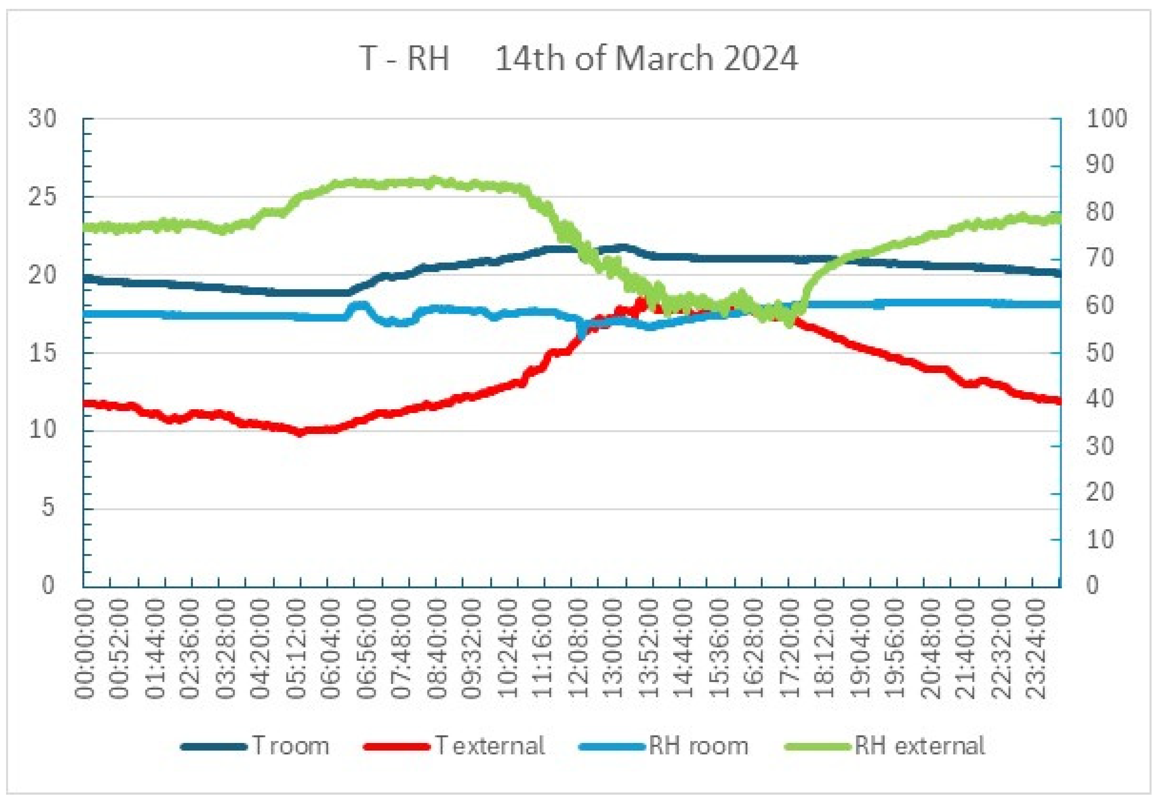
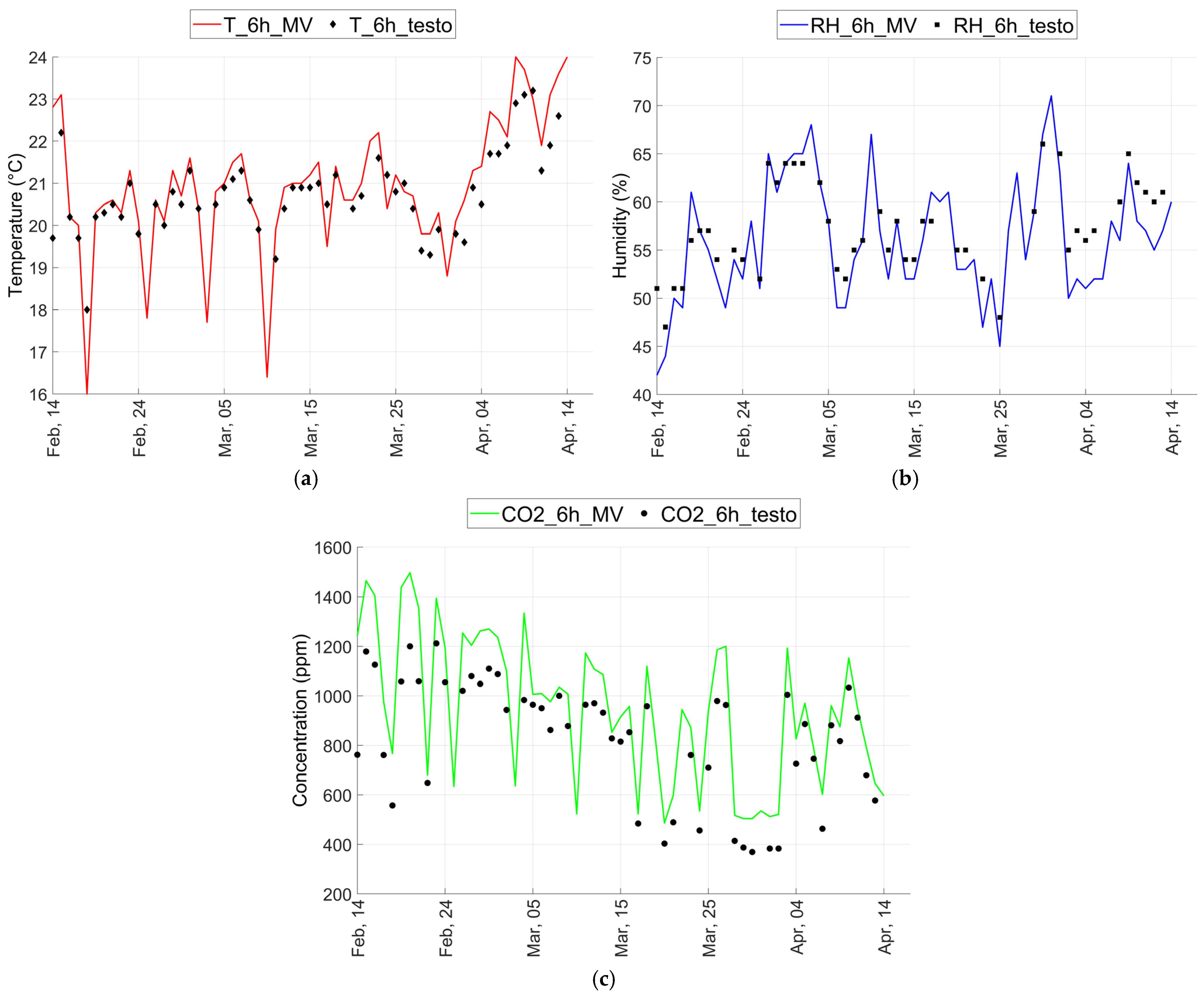
- CO2, humidity, and temperature measurements were obtained from two sensors: one located 1.70 m above the ground and the other near the ventilation machine system’s intake. The average deviations between the two sensors were approximately 0.8 K for temperature, 1% for relative humidity, and 147 ppm(v) for CO2 (Figure 14a–c).
- -
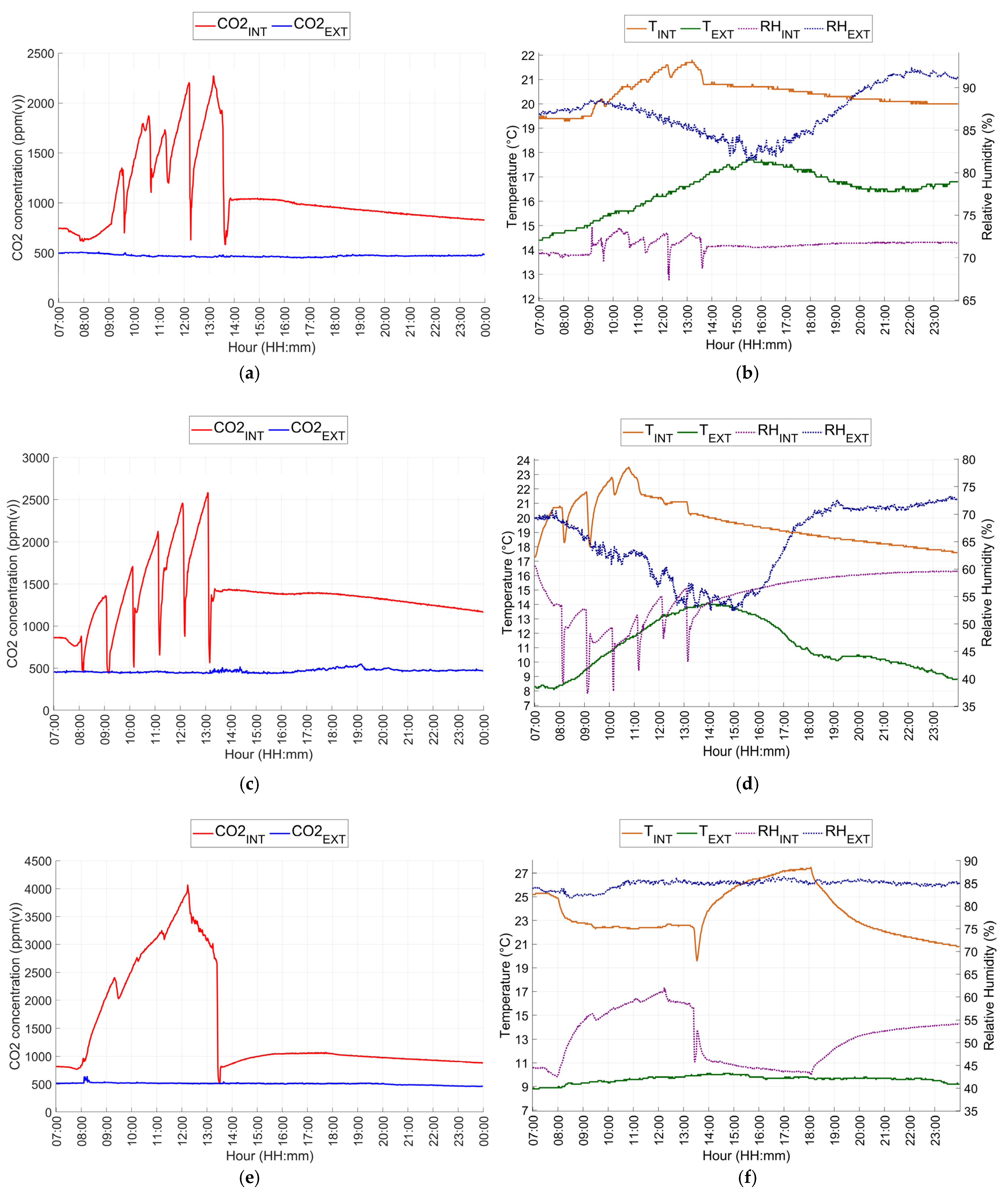
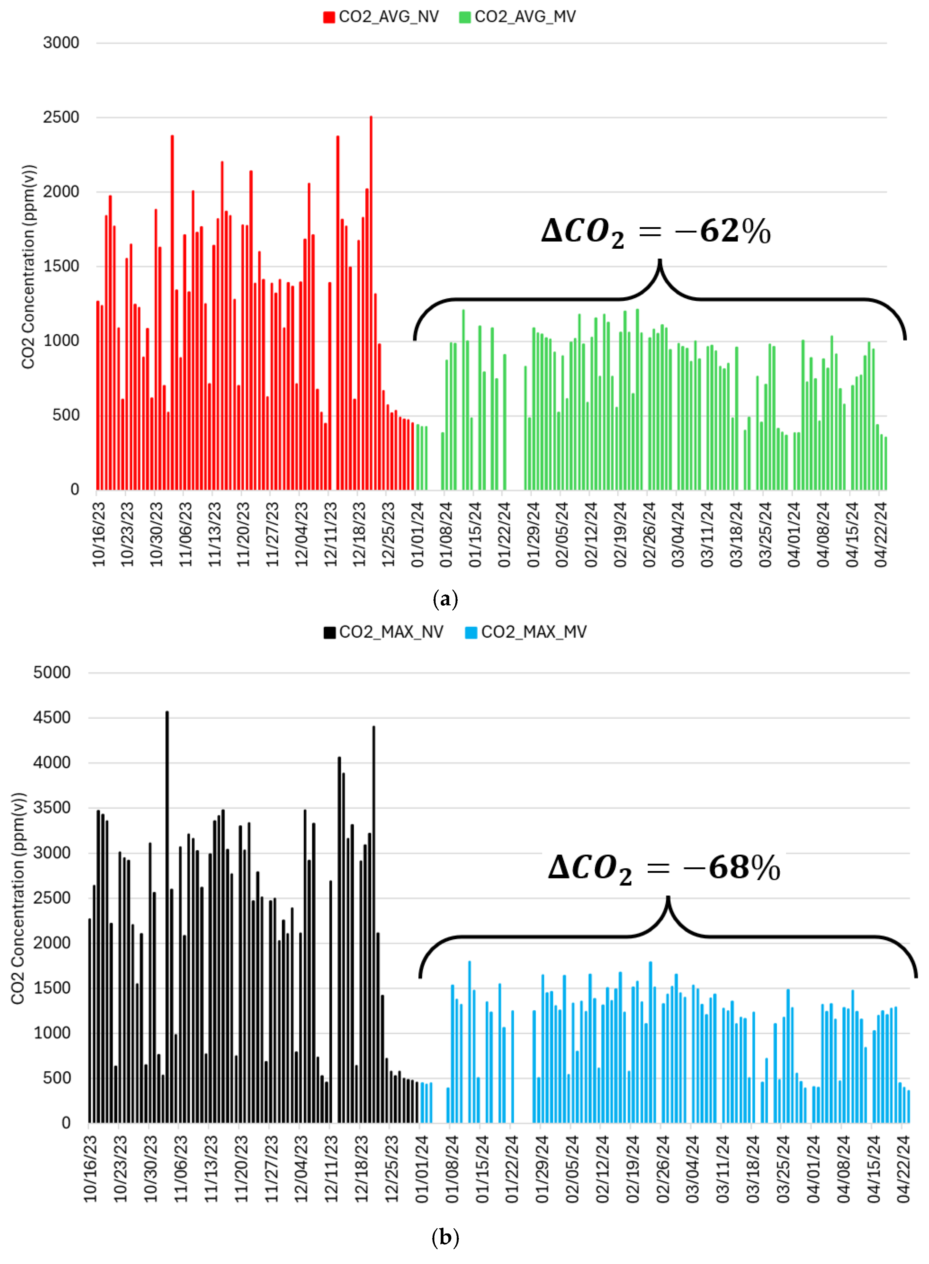
- CO2 concentrations in the classroom dropped significantly with mechanical ventilation, with peak values reaching more than 4500 ppm(v) under natural ventilation and rarely exceeding 1500 ppm(v) with mechanical ventilation. The average concentration during occupancy decreased from around 2500 ppm(v) to levels close to 1000 ppm(v) and a reduction of 62% (Figure 10a, considering mean values during the occupation period), and the daily reduction reached −68% considering the maximum daily values (Figure 10b).
- -
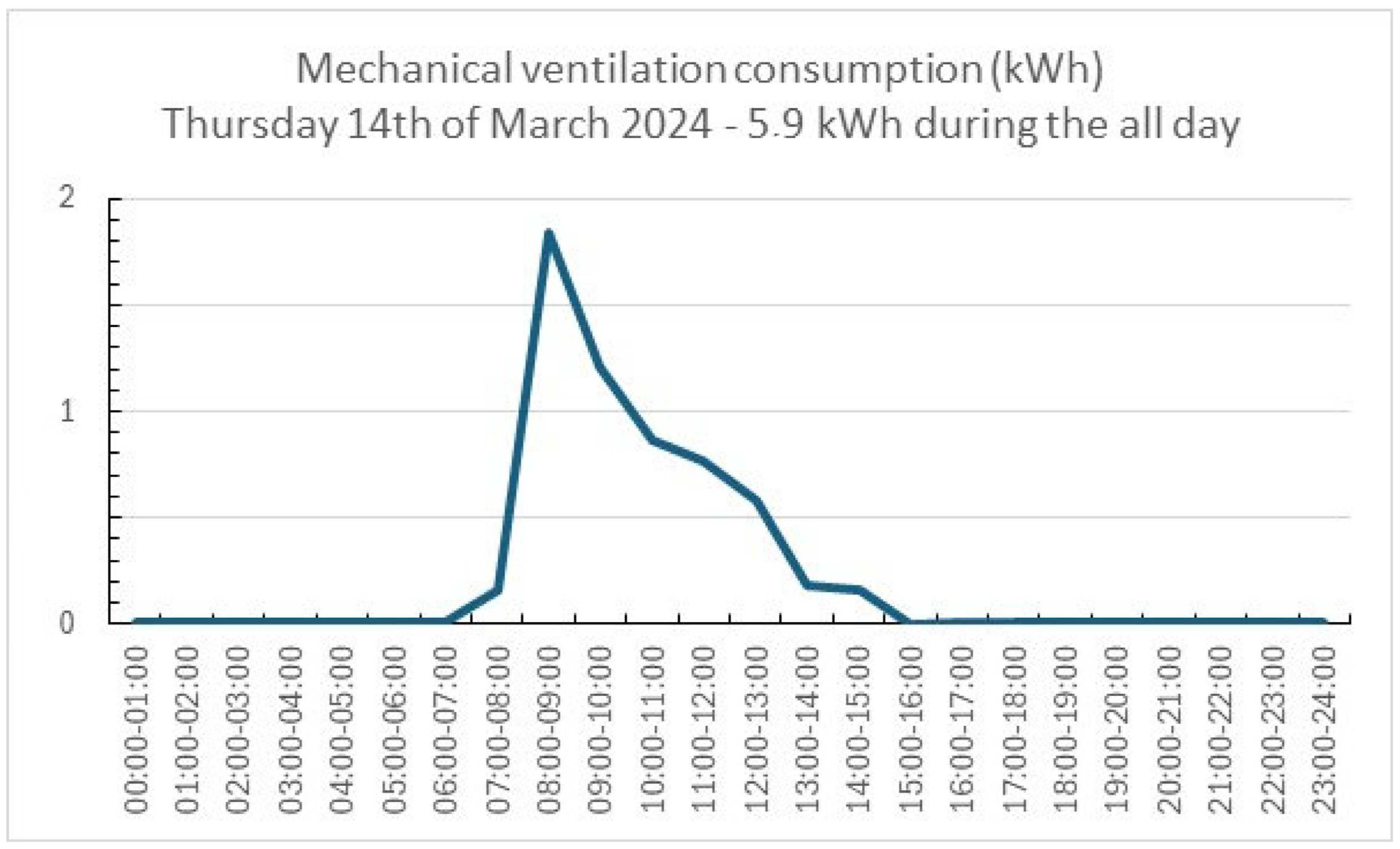
- Energy consumption by the MVHR system varied due to the use of the post-heating battery, mainly depending on external air temperature (R2 = 0.425), as the machine was set to operate at a fixed rate. Daily energy usage ranged from about 1 kWh to 11 kWh over 6 h of operation, indicating the need for variable-rate operation to reduce energy use and avoid excessive ventilation and consumption.
- -
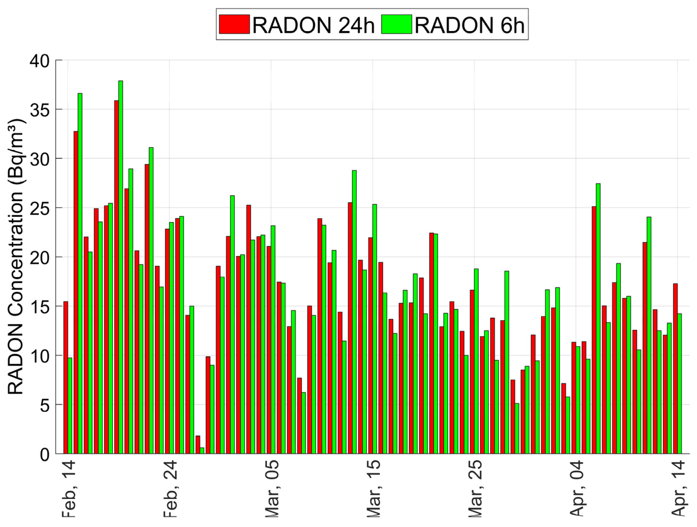
- While the MVHR system demonstrated clear benefits in managing CO2 levels, similar effects were not observed for PM2.5, VOCs, or radon. Throughout the measurement period, indoor PM2.5 levels (daily range 3–39 μg/m3) remained lower than those outside, regardless of whether the machine was on or off. No significant differences were observed in VOC levels between machine operation and downtime, with daily averages between 60 and 370 ppb. Radon levels also showed no significant change with the system on or off, with annual average values around 21 Bq/m3 and peaks reaching 56 Bq/m3 (Figure 12a,b and Figure 13). These effects may be partly attributed to the machine’s operation at neutral pressure, allowing potential pollutant infiltration from outside, even though the system is equipped with an F7/ePM1 70% filter that can capture at least 70% of finer particles, including PM1. The observed indoor PM2.5 levels mirrored those from nearby ARPAE monitoring stations outside the building.
- -
- Characterization of the environmental microbiome (microbial, bacterial, and fungal communities) and methods to support a balanced ecosystem, including compatible plant installations (green classrooms);
- -
- Control of thermohygrometric, physical, chemical, and energy parameters to enhance occupant health and reduce the built environment’s carbon footprint (decarbonization);
- -
- Improvement in psychological well-being and learning outcomes by enhancing the aesthetic, functional, and material qualities of spaces, promoting interaction among people and between individuals and their environment (interior design);
- -
- Development and prototyping of innovative educational spaces, using specific and quantitative knowledge of the various parameters that contribute to the livability of constructed spaces.
Author Contributions
Funding
Data Availability Statement
Acknowledgments
Conflicts of Interest
Appendix A

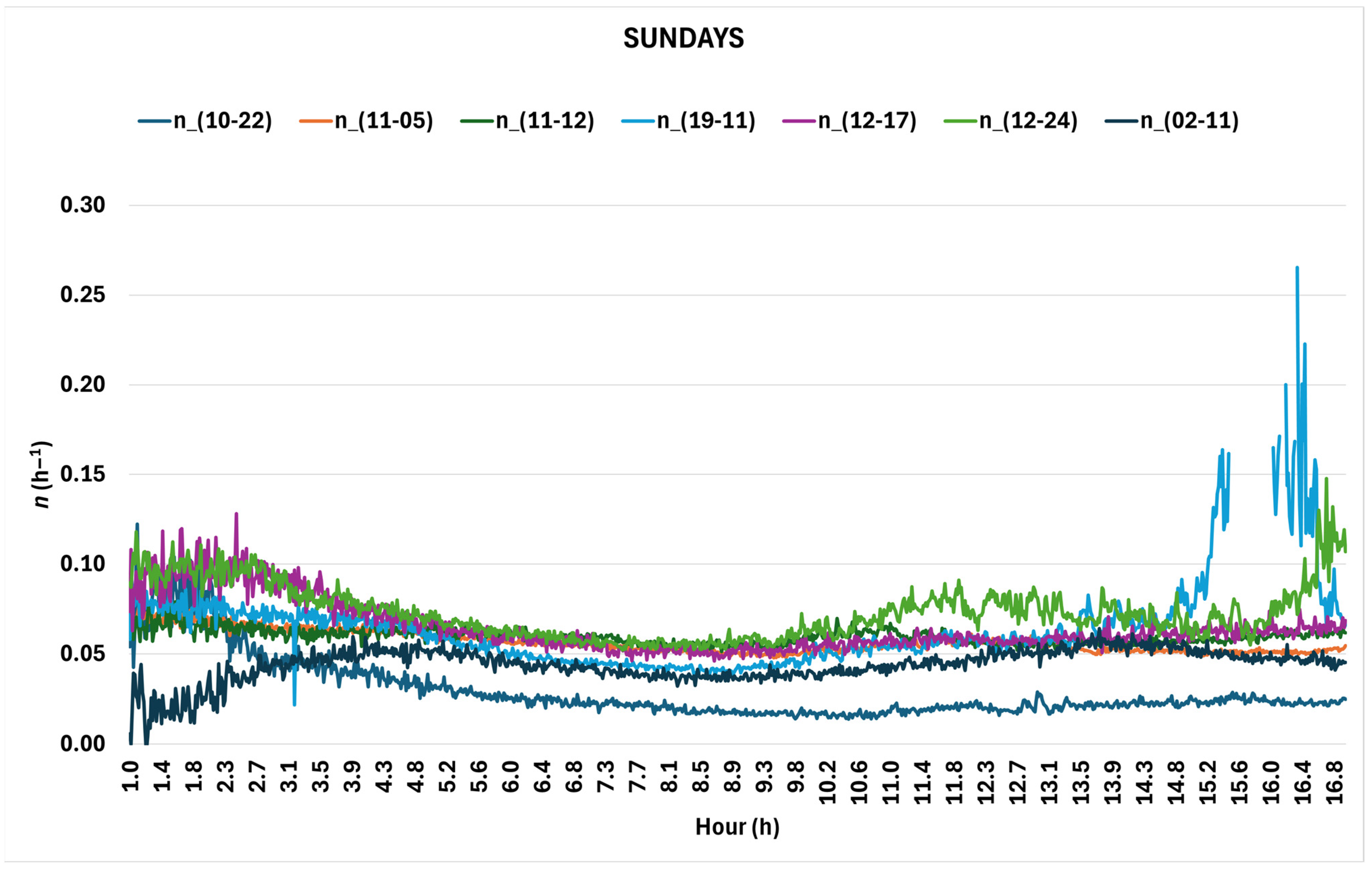
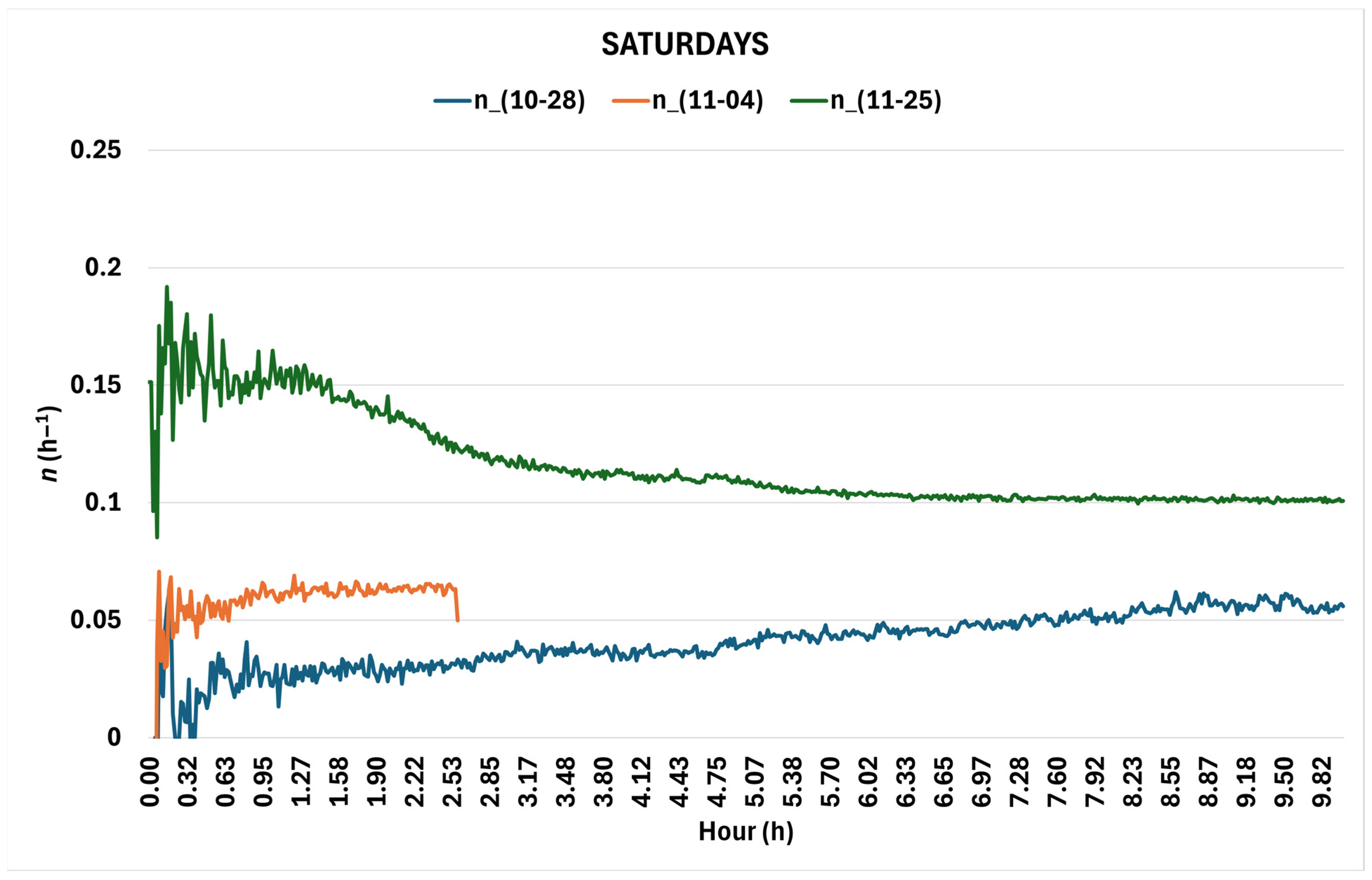
| Date | Period | Day of the Week | n (h−1) |
|---|---|---|---|
| 22 October 2023 | 07.00–0.00 | SUNDAY | 0.032 |
| 5 November 2023 | 07.00–0.00 | SUNDAY | 0.058 |
| 12 November 2023 | 07.00–0.00 | SUNDAY | 0.061 |
| 19 November 2023 | 07.00–0.00 | SUNDAY | 0.065 |
| 17 December 2023 | 07.00–0.00 | SUNDAY | 0.065 |
| 24 December 2023 | 07.00–0.00 | SUNDAY | 0.077 |
| 11 February 2024 | 07.00–0.00 | SUNDAY | 0.046 |
| 28 October 2023 | 14.00–0.00 | SATURDAY | 0.040 |
| 4 November 2023 | 14.00–0.00 | SATURDAY | 0.057 |
| 25 November 2023 | 14.00–0.00 | SATURDAY | 0.116 |
Appendix B
References
- World Health Organization (WHO). WHO Guidelines for Indoor Air Quality: Selected Pollutants; WHO Regional Office for Europe: Copenhagen, Denmark, 2010; Available online: https://iris.who.int/bitstream/handle/10665/260127/9789289002134-eng.pdf (accessed on 10 November 2024).
- United States Environmental Protection Agency (EPA). The Inside Story: A Guide to Indoor Air Quality; U.S. Environmental Protection Agency: Washington, DC, USA, 2021. Available online: https://www.epa.gov/indoor-air-quality-iaq/inside-story-guide-indoor-air-quality (accessed on 10 November 2024).
- European Parliament and Council of the European Union. Directive (EU) 2018/844 of the European Parliament and of the Council of 30 May 2018 amending Directive 2010/31/EU on the Energy Performance of Buildings and Directive 2012/27/EU on Energy Efficiency. Official Journal of the European Union, L 156/75. 2018. Available online: https://eur-lex.europa.eu/legal-content/EN/TXT/?uri=CELEX:32018L0844 (accessed on 10 November 2024).
- European Parliament and Council of the European Union. Directive (EU) 2024/1275 of the European Parliament and of the Council on the Energy Performance of Buildings aiming at Zero-Emission Buildings by 2050. Official Journal of the European Union, L 128/75. 2024. Available online: https://eur-lex.europa.eu/legal-content/EN/TXT/?uri=OJ:L_202401275 (accessed on 10 November 2024).
- McGill, G.; Oyedele, L.O.; McAllister, K. An Investigation of Indoor Air Quality, Thermal Comfort and Sick Building Syndrome Symptoms in UK Energy Efficient Homes. Smart Sustain. Built Environ. 2015, 4, 329–348. [Google Scholar] [CrossRef]
- Rostron, J. Sick Building Syndrome: A Review of Causes, Consequences and Remedies. J. Retail. Leis. Prop. 2008, 7, 291–303. [Google Scholar] [CrossRef]
- Takeda, M.; Saijo, Y.; Yuasa, M.; Kanazawa, A.; Araki, A.; Kishi, R. Relationship between Sick Building Syndrome and Indoor Environmental Factors in Newly Built Japanese Dwellings. Int. Arch. Occup. Environ. Health 2009, 82, 583–593. [Google Scholar] [CrossRef] [PubMed]
- Szczurek, A.; Maciejewska, M.; Pietrucha, T. CO2 and Volatile Organic Compounds as Indicators of IAQ. 2015. Available online: https://www.aivc.org/resource/co2-and-volatile-organic-compounds-indicators-iaq (accessed on 10 November 2024).
- Sánchez-Fernández, A.; Coll-Aliaga, E.; Lerma-Arce, V.; Lorenzo-Sáez, E. Evaluation of Different Natural Ventilation Strategies by Monitoring the Indoor Air Quality Using CO2 Sensors. Int. J. Environ. Res. Public Health 2023, 20, 6757. [Google Scholar] [CrossRef]
- Schibuola, L.; Tambani, C. Indoor Environmental Quality Classification of School Environments by Monitoring PM and CO2 Concentration Levels. Atmos. Pollut. Res. 2020, 11, 332–342. [Google Scholar] [CrossRef]
- Settimo, G.; Indinnimeo, L.; Inglessis, M.; De Felice, M.; Morlino, R.; di Coste, A.; Carriera, F.; Di Fiore, C.; Avino, P. CO2 Levels in Classrooms: What Actions to Take to Improve the Quality of Environments and Spaces. Sustainability 2024, 16, 8619. [Google Scholar] [CrossRef]
- Satish, U.; Mendell, M.J.; Shekhar, K.; Hotchi, T.; Sullivan, D.; Streufert, S.; Fisk, W.J. Is CO2 an Indoor Pollutant? Direct Effects of Low-to-Moderate CO2 Concentrations on Human Decision-Making Performance. Environ. Health Perspect. 2012, 120, 1671–1677. [Google Scholar] [CrossRef]
- Ballerini, V.; Valdiserri, P.; Krawczyk, D.A.; Sadowska, B.; Lubowicka, B.; di Schio, E.R. Design, comparison and application of artificial intelligence predictive models based on experimental data for estimating carbon dioxide concentration inside a building. Appl. Therm. Eng. 2015, 261, 125122. [Google Scholar] [CrossRef]
- Ballerini, V.; Lubowicka, B.; Valdiserri, P.; Krawczyk, D.A.; Sadowska, B.; Kłopotowski, M.; di Schio, E.R. The Energy Retrofit Impact in Public Buildings: A Numerical Cross-Check Supported by Real Consumption Data. Energies 2023, 16, 7748. [Google Scholar] [CrossRef]
- Loreti, L.; Valdiserri, P.; Garai, M. Dynamic simulation on energy performance of a school. Energy Procedia 2016, 101, 1026–1033. [Google Scholar] [CrossRef]
- Cesari, S.; Valdiserri, P.; Coccagna, M.; Mazzacane, S. The energy saving potential of wide windows in hospital patient rooms, optimizing the type of glazing and lighting control strategy under different climatic conditions. Energies 2020, 13, 2116. [Google Scholar] [CrossRef]
- Krawczyk, D.A.; Rodero, A.; Gładyszewska-Fiedoruk, K.; Gajewski, A. CO2 Concentration in Naturally Ventilated Classrooms Located in Different Climates—Measurements and Simulations. Energy Build. 2016, 129, 491–498. [Google Scholar] [CrossRef]
- Chatzidiakou, L.; Archer, R.; Beale, V.; Bland, S.; Carter, H.; Castro-Faccetti, C.; Burridge, H.C. Schools’ air quality monitoring for health and education: Methods and protocols of the SAMHE initiative and project. Dev. Built Environ. 2023, 16, 100266. [Google Scholar] [CrossRef]
- Dimitroulopoulou, S.; Dudzińska, M.R.; Gunnarsen, L.; Hägerhed, L.; Maula, H.; Singh, R.; Toyinbo, O.; Haverinen-Shaughnessy, U. Indoor Air Quality Guidelines from across the World: An Appraisal Considering Energy Saving, Health, Productivity, and Comfort. Environ. Int. 2023, 178, 108127. [Google Scholar] [CrossRef] [PubMed]
- Lowther, S.D.; Dimitroulopoulou, S.; Foxall, K.; Shrubsole, C.; Cheek, E.; Gadeberg, B.; Sepai, O. Low Level Carbon Dioxide Indoors—A Pollution Indicator or a Pollutant? A Health-Based Perspective. Environments 2021, 8, 125. [Google Scholar] [CrossRef]
- BS EN 16798-1:2019; Energy Performance of Buildings—Ventilation for Buildings—Part 1: Indoor Environmental Input Parameters for Design and Assessment of Energy Performance of Buildings Addressing Indoor Air Quality, Thermal Environment, Lighting and Acoustics. British Standards Institution: London, UK, 2019.
- National Oceanic and Atmospheric Administration (NOAA). Climate Change: Atmospheric Carbon Dioxide. Available online: https://www.climate.gov/news-features/understanding-climate/climate-change-atmospheric-carbon-dioxide (accessed on 10 November 2024).
- Madureira, J.; Paciência, I.; Pereira, C.; Teixeira, J.P.; de O Fernandes, E. Indoor Air Quality in Portuguese Schools: Levels and Sources of Pollutants. Indoor Air 2016, 26, 526–537. [Google Scholar] [CrossRef] [PubMed]
- Lucialli, P.; Marinello, S.; Pollini, E.; Scaringi, M.; Sajani, S.Z.; Marchesi, S.; Cori, L. Indoor and Outdoor Concentrations of Benzene, Toluene, Ethylbenzene and Xylene in Some Italian Schools Evaluation of Areas with Different Air Pollution. Atmos. Pollut. Res. 2020, 11, 1998–2010. [Google Scholar] [CrossRef]
- Seltenrich, N. Clearing the Air: Gas Stove Emissions and Direct Health Effects. Environ. Health Perspect. 2024, 132, 022001. [Google Scholar] [CrossRef]
- World Health Organization (WHO). Household Air Pollution and Health; WHO: Geneva, Switzerland, 2023; Available online: https://www.who.int/news-room/fact-sheets/detail/household-air-pollution-and-health (accessed on 11 November 2024).
- World Health Organization (WHO). WHO Global Air Quality Guidelines; WHO: Geneva, Switzerland, 2021; Available online: https://www.who.int/publications/i/item/9789240034228 (accessed on 11 November 2024).
- Tofful, L.; Canepari, S.; Sargolini, T.; Perrino, C. Indoor Air Quality in a Domestic Environment: Combined Contribution of Indoor and Outdoor PM Sources. Build. Environ. 2021, 202, 108050. [Google Scholar] [CrossRef]
- Cai, C.; Sun, Z.; Weschler, L.B.; Li, T.; Xu, W.; Zhang, Y. Indoor Air Quality in Schools in Beijing: Field Tests, Problems and Recommendations. Build. Environ. 2021, 205, 108179. [Google Scholar] [CrossRef]
- Settimo, G.; Manigrasso, M.; Avino, P. Indoor Air Quality: A Focus on the European Legislation and State-of-the-Art Research in Italy. Atmosphere 2020, 11, 370. [Google Scholar] [CrossRef]
- Zeeb, H.; Shannoun, F.; Organization, W.H. WHO Handbook on Indoor Radon: A Public Health Perspective; WHO: Geneva, Switzerland, 2009; ISBN 978-4-938987-94-7. [Google Scholar]
- Gaskin, J.; Coyle, D.; Whyte, J.; Krewksi, D. Global Estimate of Lung Cancer Mortality Attributable to Residential Radon. Environ. Health Perspect. 2018, 126, 057009. [Google Scholar] [CrossRef] [PubMed]
- Indoor Radon Concentration Map. Available online: https://remap.jrc.ec.europa.eu/Atlas.aspx?layerID=3 (accessed on 10 November 2024).
- Dubois, G.; Bossew, P.; Tollefsen, T.; De Cort, M. First Steps towards a European Atlas of Natural Radiation: Status of the European Indoor Radon Map. J. Environ. Radioact. 2010, 101, 786–798. [Google Scholar] [CrossRef] [PubMed]
- Jeong, J.; Cho, K. Experimental Study on CO2 and Radon Mitigations in an Apartment Using a Mechanical Ventilation System. Buildings 2023, 13, 1439. [Google Scholar] [CrossRef]
- Dovjak, M.; Virant, B.; Krainer, A.; Zavrl, M.Š.; Vaupotič, J. Determination of Optimal Ventilation Rates in Educational Environment in Terms of Radon Dosimetry. Int. J. Hyg. Environ. Health 2021, 234, 113742. [Google Scholar] [CrossRef]
- Italy. Legislative Decree D.Lgs 101/2020. Attuazione della Direttiva 2013/59/Euratom, Che Stabilisce Norme Fondamentali di Sicurezza Relative alla Protezione Contro i Pericoli Derivanti Dall’esposizione alle Radiazioni Ionizzanti; Gazzetta Ufficiale della Repubblica Italiana: Rome, Italy, 2020; Available online: https://www.gazzettaufficiale.it/eli/id/2020/08/12/20G00121/sg (accessed on 10 November 2024).
- European Union. Council Directive 2013/59/EURATOM. Laying Down Basic Safety Standards for Protection Against the Dangers Arising from Exposure to Ionising Radiation; Official Journal of the European Union: Brussels, Belgium, 2014; Available online: https://eur-lex.europa.eu/eli/dir/2013/59/oj (accessed on 10 November 2024).
- Conceição, E.Z.; Farinho, J.P.; Lúcio, M.J. Evaluation of indoor air quality in classrooms equipped with cross-flow ventilation. Int. J. Vent. 2012, 11, 53–68. [Google Scholar] [CrossRef]
- Conceição, E.Z.E.; Lúcio, M.M.; Ruano, A.E.B.; Crispim, E.M. Development of a temperature control model used in HVAC systems in school spaces in Mediterranean climate. Build. Environ. 2009, 44, 871–877. [Google Scholar] [CrossRef]
- Khovalyg, D.; Kazanci, O.B.; Halvorsen, H.; Gundlach, I.; Bahnfleth, W.P.; Toftum, J.; Olesen, B.W. Critical review of standards for indoor thermal environment and air quality. Energy Build. 2020, 213, 109819. [Google Scholar] [CrossRef]
- Berger, C.; Mahdavi, A.; Azar, E.; Bandurski, K.; Bourikas, L.; Harputlugil, T.; Schweiker, M. Reflections on the evidentiary basis of indoor air quality standards. Energies 2022, 15, 7727. [Google Scholar] [CrossRef]
- SYMBIEN. School Symbiotic Environments. Available online: https://cias-ferrara.it/projects/symbien/ (accessed on 10 November 2024).
- Testo 160 IAQ—Wi-Fi Data Logger. Technical Datasheet. Available online: https://static.testo.com/image/upload/US/testo-160-iaq-datasheet-us.pdf (accessed on 9 November 2024).
- AIRTHINGS VIEW PLUS Sensor. Thecnical Datasheet. Available online: https://www.airthings.com/hubfs/Website/Product%20Sheets/view-plus/view-plus-product-sheet-EN.pdf?hsLang=en-us (accessed on 9 November 2024).
- Aldes, Product Datasheet. Available online: https://www.aldes.it/ (accessed on 9 November 2024).
- Volterra, V. Fluctuations in the Abundance of a Species considered Mathematically. Nature 1926, 118, 558–560. [Google Scholar] [CrossRef]
- Esfehani, H.H.; Schäuble, J.; Paul, E.; Bohne, D. Simulation and analysis of load shifting and energy saving potential of CO2-based demand-controlled ventilation in a sports training center. IOP Conf. Ser. Mater. Sci. Eng. 2019, 609, 052042. [Google Scholar] [CrossRef]
- Stönner, C.; Edtbauer, A.; Williams, J. Real-world volatile organic compound emission rates from seated adults and children for use in indoor air studies. Indoor Air 2018, 28, 164–172. [Google Scholar] [CrossRef] [PubMed]
- Bella, G.; Massidda, C.; Mattana, P. The relationship among CO2 emissions, electricity power consumption and GDP in OECD countries. J. Policy Model. 2014, 36, 970–985. [Google Scholar] [CrossRef]
- Valdiserri, P.; Ballerini, V.; Rossi di Schio, E. Interpolating functions for CO2 emission factors in dynamic simulations: The special case of a heat pump. Sustain. Energy Technol. Assess. 2022, 53, 102725. [Google Scholar] [CrossRef]
- Dafdsf ARPAE, Emilia-Romagna Regional Environmental Protection Agency. Available online: https://www.arpae.it/it (accessed on 9 November 2024).
- Dext3r Web App. Available online: https://simc.arpae.it/dext3r/ (accessed on 9 November 2024).
- Air Quality in Emilia-Romagna. Available online: https://sdati-test.datamb.it/arex/ (accessed on 9 November 2024).
- Pei, G.; Rim, D.; Schiavon, S.; Vannucci, M. Effect of Sensor Position on the Performance of CO2-Based Demand Controlled Ventilation. Energy Build. 2019, 202, 109358. [Google Scholar] [CrossRef]


| Variable | Range | Accuracy | Resolution |
|---|---|---|---|
| Temperature | 0–50 °C | ±0.1 K | 0.1 K |
| Humidity | 0–100% | ±2% (range 20–80% at 25 °C) | 0.1% |
| CO2 | 0–5000 ppm(v) | ±(50 ppm(v) + 3% m.v.) | 1 ppm(v) |
| Variable | Range | Accuracy |
|---|---|---|
| Temperature | 4–40 °C | 0.5 K |
| Humidity | Up to 85% | 3% |
| Pressure | 0.6 hPa | |
| Radon | 0–20,000 Bq/m3 | ±10% m.v. |
| Particulate (PM2.5) | 0–500 μg/m3 | ±5 (μg/m3 +15% m.v.), range 0–150 μg/m3 |
| VOCs | 0–10,000 ppb | - |
| CO2 | 400–5000 ppm | ±(50 ppm(v) + 5% m.v.) |
| Length | 8.47 m |
| Width | 5.75 m |
| Ceiling height | 3.23 m |
| Maximum height | 5.15 m |
| Floor area | 48.7 m2 |
| Volume | 170 m3 |
| Heat recovery efficiency 1 | 80% |
| Nominal power (excluding electrical post-heating) | 377 W |
| Nominal external pressure | 50 Pa |
| Fan efficiency | 49.3% |
| Specific power (SFPint) | 1189 W/(m3/s) |
| Filters | F7/ePM1 70% for extraction and fresh air |
| Sound power level 1 | 56 dB(A) |
Disclaimer/Publisher’s Note: The statements, opinions and data contained in all publications are solely those of the individual author(s) and contributor(s) and not of MDPI and/or the editor(s). MDPI and/or the editor(s) disclaim responsibility for any injury to people or property resulting from any ideas, methods, instructions or products referred to in the content. |
© 2025 by the authors. Licensee MDPI, Basel, Switzerland. This article is an open access article distributed under the terms and conditions of the Creative Commons Attribution (CC BY) license (https://creativecommons.org/licenses/by/4.0/).
Share and Cite
Ballerini, V.; Coccagna, M.; Bisi, M.; Volta, A.; Droghetti, L.; Rossi di Schio, E.; Valdiserri, P.; Mazzacane, S. The Role of Mechanical Ventilation in Indoor Air Quality in Schools: An Experimental Comprehensive Analysis. Buildings 2025, 15, 869. https://doi.org/10.3390/buildings15060869
Ballerini V, Coccagna M, Bisi M, Volta A, Droghetti L, Rossi di Schio E, Valdiserri P, Mazzacane S. The Role of Mechanical Ventilation in Indoor Air Quality in Schools: An Experimental Comprehensive Analysis. Buildings. 2025; 15(6):869. https://doi.org/10.3390/buildings15060869
Chicago/Turabian StyleBallerini, Vincenzo, Maddalena Coccagna, Matteo Bisi, Antonella Volta, Lorenzo Droghetti, Eugenia Rossi di Schio, Paolo Valdiserri, and Sante Mazzacane. 2025. "The Role of Mechanical Ventilation in Indoor Air Quality in Schools: An Experimental Comprehensive Analysis" Buildings 15, no. 6: 869. https://doi.org/10.3390/buildings15060869
APA StyleBallerini, V., Coccagna, M., Bisi, M., Volta, A., Droghetti, L., Rossi di Schio, E., Valdiserri, P., & Mazzacane, S. (2025). The Role of Mechanical Ventilation in Indoor Air Quality in Schools: An Experimental Comprehensive Analysis. Buildings, 15(6), 869. https://doi.org/10.3390/buildings15060869