Abstract
In the context of model updating of bridge structures, dynamic approaches are currently dominant. This is mainly due to the opportunity of performing dynamic tests under environmental and traffic loadings, without putting the bridges out of service. Several techniques have been proposed in the literature to control and address the relevant model updating workflow. These methods typically consider the structural frequencies, or a combination of frequencies with vibration modes. Dissipative properties are, on the contrary, more rarely considered in updating procedures, given their strong dependence on the amplitude of the vibrations and on the type of forcing load. In this work, six ruling objective functions are considered for the dynamic model updating of girder bridge structures. The first one, taken from the literature, is a widely used function based on discrepancies among numerical and experimental frequencies. Two additional functions, also derived from the existing literature, are subsequently considered: one focuses on vibration modes, utilizing the Modal Assurance Criterion (MAC), and the other incorporates both structural frequencies and mode shapes, deploying the Modal Flexibility Matrix (MFM). Three novel objective functions are introduced, which are adaptations of the previously mentioned ones, with alternative applications of MAC and MFM. These six functions are analyzed and discussed through two comprehensive experimental case studies, in which the relative weights of the specific function terms are also investigated. A quantitative selection criterion is proposed and examined in order to choose the most suitable objective function based on identifiability. The method implementation, leveraging second-order derivatives, is executed via a finite difference scheme.
1. Introduction
Model updating is a process involving the modification and enhancement of a numerical structural model, typically based on experimental test results, to achieve a reliable representation of structural behavior under specific loading conditions. This process addresses an inverse problem that allows for the adjustment of model parameters to improve the alignment between predictions and experimental results, thereby reducing simulation biases, uncertainties, and errors.
In structural numerical simulations, biases, uncertainties, and errors arise from various sources, and the following classification is currently usually accepted in the literature [1,2,3,4]:
- Modeling errors, which stem from inaccurate or simplifying assumptions in the model definition; these can include uncertainties in the mathematical equations governing the model (model–structure errors), such as geometric simplifications or kinematic and static assumptions; or approximate boundary conditions and model characteristics (model–parameter errors), like simplified restraint and load definitions or erroneous modeling of structural members; or approximate discretization and simplification of the modeled system (model–order errors), such as truncation errors or mesh discretization.
- Parameter value errors, arising from inaccurate assumptions regarding the values of the parameters that govern the structural response, such as material properties as well as member dimensions and stiffnesses; these may not be precisely known or may exhibit spatial variability that are too significant to be accurately described.
- Numerical software/hardware errors, which stem from the algorithms used to solve the model governing equations, including rounding errors and iterative convergence issues.
Moreover, since model updating relies on measured data, an important source of uncertainty is also that related to measurement or experimental error, which can manifest as random noise or systematic error due to equipment imperfections or subsequent signal processing [5]. For this reason, optimal sensor placement is a research branch strictly connected to model updating [6].
Even for large structures [7], model updating typically addresses errors in parameter values, employing various techniques to accurately calibrate the primary parameters of the model and reduce discrepancies between numerical and experimental results. Substructures are often used to reduce the computing time [8,9]. Model updating can also be used for damage identification [10,11,12].
In particular, methods can be categorized into two main classes. The first one concerns deterministic methods, which involve sensitivity analysis of the parameters governing the structural response and iterative or searching techniques to calibrate their correct values. The second class encompass uncertain parameters based on probabilistic approaches. Some applications can be found in Refs. [13,14], and an interested reader can refer to the available literature [15,16].
This paper focuses on deterministic sensitivity methods. In such methods, the main difficulties concern the choice of the parameters to be modified and the objective function to be adopted. Using data from construction monitoring can simplify complex multi-variable problems arising when traditional model updating approaches are adopted [17]. Referring to the specific case of dynamic model updating, linear models are commonly assumed, but some strategic approaches considering nonlinearities have been proposed [18]. Artificial intelligence has also been used in this context [19,20], trying to reduce additional complex mathematical calculations.
In this study, six objective functions are considered for the dynamic model updating of girder bridge structures. The first function, derived from the literature, is a widely used objective function based on the discrepancies between numerical and experimental frequencies. Two additional functions from existing studies are also adopted: one considers vibration modes through the Modal Assurance Criterion (MAC), and the other combines both frequencies and mode shapes using the Modal Flexibility Matrix (MFM). The remaining three objective functions are new proposals, and are obtained by properly combining MAC and MFM to better reflect different aspects of the updating process. These six objective functions are compared and evaluated using two full-scale experimental case studies, with varying weights assigned to the components of each function. Furthermore, a quantitative criterion is introduced for selecting the optimal objective function based on its identifiability performance.
2. Dynamic Model Updating and Definition of the Objective Functions
After a discussion on the general concepts related to model updating procedures and some insights concerning the relevant architectures, the adopted objective functions are discussed.
2.1. General Concepts
According to the descriptions provided in Refs. [3,4], a structural model can be viewed as an input–output function . This function takes an input vector , which may represent various loadings acting on the structure, and produces a set of output variables that characterize the mechanical behavior of the structural system. These output variables include displacements, strains, stresses, modal frequencies, and other relevant metrics. Function is inherently dependent on the structural properties of the system, which are defined by a finite set of parameters that encapsulate the characteristics of the structure. In other words:
However, model updating procedures are often based on output results that are independent of the input data , as typically done in dynamic model updating, where output quantities are often derived features, such as natural frequencies or modal shapes, i.e.,
To be noted is that the parameter vector spans a subset of values, representing not a single model, but an entire class of models, i.e., the model class , and each model within this model class provides a mapping from the model parameter space to the output space.
In this framework, deterministic model updating involves determining the optimal values of the model parameters, , that minimize the difference between model predictions and the corresponding experimentally obtained data . This difference is quantified by a cost function that needs to be minimized. Therefore, model updating is a constrained optimization problem, where the objective function to minimize reflects the discrepancy between the predicted numerical data and the experimentally observed data.
The general architecture of a sensitivity-based model updating procedure is discussed in the following section, whereas the subsequent one is dedicated to the adopted objective functions.
2.2. Model Updating Procedure
The following steps are usually required in a model updating process:
- Model class selection;
- Initial model definition;
- Output selection;
- Objective function definition;
- Sensitivity parameter selection;
- Parameter calibration (updating).
The first step involves selecting the type of model to describe the mechanical response of the structure, including all simplifying assumptions regarding geometric or mechanical characteristics of the structure. In this work, finite element (FE) models are used, based on linear elastic frame and shell formulations, as discussed in detail in Section 3.
Once the model class has been selected, the initial model of the structure is created (step 2) using the initial values of all model parameters, such as material properties and element dimensions. These values are typically derived from design documentation or from in situ and laboratory tests on selected specimens. On the one hand, the initial model should be as accurate as possible to minimize modeling errors and the discrepancy between numerical predictions and experimental results. However, on the other hand, the model must not be overly complex or dependent on too many parameters, as this can complicate and destabilize the updating process. Achieving a good balance between accuracy and complexity may require modifications to the model class and the iterative switch between the model class selection (step 1) and the initial model definition (step 2).
To avoid the ill-conditioning of the updating process, steps 3, 4, and 5 play a crucial role as, in general, updating all model parameters and optimizing the prediction of all output variables is unfeasible.
First, a specific set of model features must be selected as target output variables to be improved (step 3). For instance, instead of considering all natural frequencies and mode shapes, only the first most relevant eigenmodes are selected. This choice, certainly, also depends on the experimental data available as reference.
Then, the objective function to be minimized is defined to mathematically describe the misfit between the selected numerical outputs and the corresponding experimental results (step 4). This usually assumes the form of a weighted normalized square root mean square (RMS) function of the discrepancies, such as:
where and are the output variable and corresponding experimental data, respectively, and is the weight associated with the normalized residuals. This weight is a measure of the importance of the variable in the objective function, and is selected relying on the confidence that the analyst has in the corresponding measured data and in the capability of the model class in reproducing that data. The weights can be set as inversely proportional to the observed data standard deviations, when available. However, these are commonly determined based on engineering judgment.
It should be noted that the RMS in Equation (3) represents the effective value of the normalized error. This implies that, if the term in parentheses assumes the same value, namely, , for all modes, and the weights are all equal to 1, the objective function will yield exactly , which consistently matches the effective value.
Since several types of data with different characteristics can be simultaneously used as output variables, they can either be combined into one single objective function or a multi-objective optimization scheme can be considered. The latter avoids the effort of weighting the individual variables, but requires greater computational capabilities and is often avoided by professionals. Therefore, a single objective function approach is followed in this work.
After defining the objective function, sensitivity analyses are conducted to identify the model parameters that significantly influence the structural response (step 5). Only these key parameters are updated in the final step of the procedure, so as to avoid ill-conditioning. The chosen objective function serves as a metric to quantify the influence of each parameter, and two techniques can be employed. The first technique is the subset selection, which involves selecting parameters based on the orthogonality principle, i.e., each selected parameter influences specific output variables that are not affected by other parameters. This ensures that, in an iterative process, updating one parameter does not alter the outputs associated with the other parameters. The second technique is the parameter clustering, where parameters that influence the same output variables are grouped and updated together during the process.
Finally, the selected parameters of the model are updated (step 6) by minimizing the objective function, given by the chosen measure of the difference between numerical response and experimental outcomes.
The study in this work focuses on the steps 3 and 4 of the model updating procedure, involving the choice of the output variables to be monitored and the definition of the objective function. Specifically, the dynamic response of girder bridges is considered, and six different alternative objective functions are used, as detailed in the following subsection.
2.3. Adopted Objective Functions
Considering the steps 3 and 4 of the list displayed in the previous subsection, and referring to the specific case of dynamic model updating, three types of quantities are here considered as output variables to control the agreement between numerical and experimental results. These are obtained from the eigenvalue modal analysis of the structure and, for the general natural mode, are:
- Natural frequency, ;
- Vibration mode shape, ;
- Modal flexibility matrix, .
In this context, the vibration mode shape refers to a sub-vector of the complete mode shape vector: this contains only the degrees of freedom of the nodes corresponding to the experimentally monitored displacements. These sub-vectors are also used to construct the modal flexibility matrix, which couples the effects of both frequencies and mode shapes. When expressed independently for each natural mode, this results in [13,21]:
To be noted is that, while other output quantities, such as the modal strain energy [4], could be considered, these are more complex to compute, particularly from experimental measurements. Consequently, this study focuses exclusively on the simplest variables that can be straightforwardly computed in any application. Moreover, damping properties are not used in this work, since these are often affected by large variations in real-life applications [22,23].
To define the adopted objective functions, two mathematical operations are here introduced: the MAC (modal assurance criterion) [24] and the Frobenius norm of a matrix [25]. The MAC is computed between the numerical mode shape and the corresponding experimental counterpart as:
whereas, depending on the assumptions, the Frobenius norm is applied either to the numerical modal flexibility matrix , or its experimental counterpart , or their difference. For the general matrix , it results as:
It should be noted that, since modal shapes are uniquely determined except for a scaling factor, it is essential to ensure consistent scaling of numerical and experimental modal vectors when calculating the MFM matrix (as can be easily demonstrated, MAC does not depend on mode scaling). In this study, the adopted normalization considers a unit value for the norm of the scaled modal vector.
Hence, the six following expressions are here assumed as objective functions :
Hereafter, these functions are conveniently referred to by using the acronyms in the brackets. Function f (Equation (7)) is widely adopted in the literature (e.g., [26,27]), since experimental frequency values are more easily determined than other outputs. This function represents the weighted RMS of the normalized difference between numerical and experimental natural frequencies. Functions MAC1 and MFM1 (Equations (8) and (10)) are also derived from the literature ([26] and [13], respectively). They provide a dimensionless measure of the error in terms of mode shapes and a combination of frequencies and mode shapes, respectively, using for the latter the modal flexibility. However, these expressions are not based on an RMS definition. For MAC1, it can be easily proven that, when all the terms of the summation assume the same value, the function returns overall values without a straightforward interpretation, potentially leading to underestimation or overestimation of the total error. To address this issue, the alternative MAC2 (Equation (9)) is here proposed.
Function MFM1 (Equation (10)), related to the modal flexibility matrix, is not affected by the same problem. However, two alternative RMS-based functions, MFM2 and MFM3 (Equations (11) and (12)), are proposed, and their behavior is investigated: MFM2 considers the difference between the norms of the numerical and experimental counterparts, while MFM3 computes the norm of the difference matrix. Essentially, MFM3 is simply a variation on the way the terms from the various mode shapes are added together, whereas MFM2 introduces a new definition of the error and is intended to provide a global measure of the match between modes, similarly to MAC, but with MFM (and, therefore, also considering frequencies).
The characteristics of the six objective functions are summarized in Table 1.

Table 1.
Summary of the adopted objective functions.
A quantitative criterion is here introduced for choosing the objective function in which the optimal value of the parameter is best identifiable. This relies on the computation of the second-order derivative of the total error given by the function with respect to the varied parameter , i.e.,
Since this derivative represents the local curvature of the function , a higher value attained at the minimum of the curve indicates that its identification is easier:
These second-order derivatives are here computed numerically, by exploiting a four-point finite difference scheme [28].
3. Case Studies
The selected six objective functions are applied to two case studies to examine the impact of the different choices. The analyzed structures are two highway girder bridges, referred to as “Bridge A” and “Bridge B”, located in central Italy, each with distinct characteristics. Bridge A is a prestressed reinforced concrete (RC) bridge constructed in the late 1960s, while Bridge B is a newly built composite steel–concrete bridge. The following subsections provide detailed descriptions for both structures of the characteristics of the FE models used for numerical computations and the installed monitoring systems.
For both bridges, in the numerical models, structural elements belonging to the deck and the piers were modeled by discretizing them into several FEs. Their size has been properly chosen basing on preliminary converge analyses, whose results are not included in this paper for the sake of brevity.
3.1. Bridge A
Bridge A (Figure 1) consists of two independent structures supporting two carriageways, each constructed with a prestressed RC six-span girder deck. Each deck is 28 m long and comprises four I-shaped simply supported beams, transversely connected by five I-section cross beams (Figure 2). The deck slab is 20 cm thick and is connected only to the main longitudinal beams. Additionally, the slab is bordered by two RC curbs. The piers have an RC box section, and the abutments are made of a prismatic RC section.
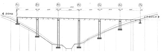
Figure 1.
Longitudinal section of Bridge A (adapted from the original drawing).
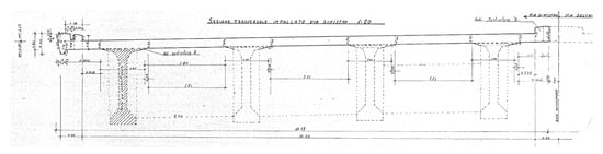
Figure 2.
Transverse section of the deck of Bridge A (adapted from the original drawing).
The bridge model is developed in SAP2000 [29], using frame FEs for all structural members, i.e., the main beams of the deck, including the slab, the cross beams, the curbs, and the piers (Figure 3). The connection between the longitudinal and the transverse cross beams of the deck is ensured by the definition of FE mesh, which divides the longitudinal beams at the intersections with the cross beams. A similar approach is used to connect the FEs representing the other structural members to the structure. The deck is connected to the piers and abutments using a two-node link system: a set of fully rigid links connects the mesh nodes at the pier cap to the mesh nodes at the intrados of each bearing, and another set of rigid links, representing the bearings, connects these nodes to those at the intrados of the main longitudinal beams. These latter restrict only specific translational degrees of freedom of the connected nodes, according to the bearing features. Pier bottoms are fully restrained. The impact of the soil layers is not considered because the mechanical properties of the soil show that it can be modeled as a simple fully restraint. Since the spans are simply supported, and the coupling given by the piers and other secondary elements was evanescent during the experimental investigations, the FE model includes only span #4 of one carriageway, which is the span where sensors have been placed during the dynamic measurements. Finally, all the dead loads, such as bridge deck pavement, are taken into account as additional equivalent distributed line load applied to the frame FEs representing the deck.
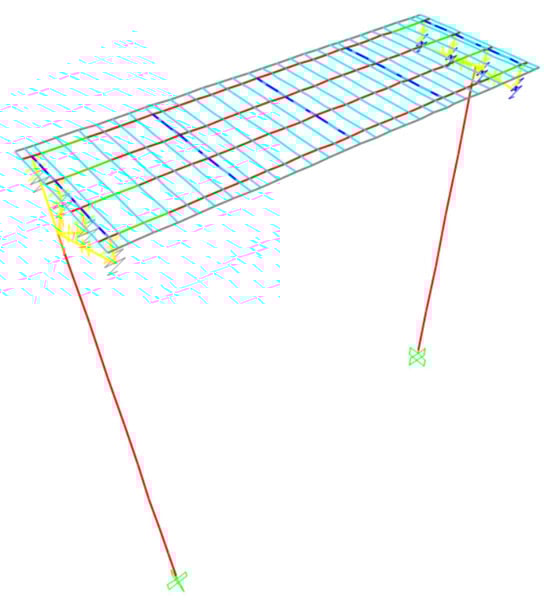
Figure 3.
Finite element model developed for Bridge A.
The monitored points during the experimental dynamic measurements are depicted in Figure 4. The monitoring system includes seven triaxial MEMS accelerometers (A1 to A7), characterized by a sampling frequency of 250 Hz.
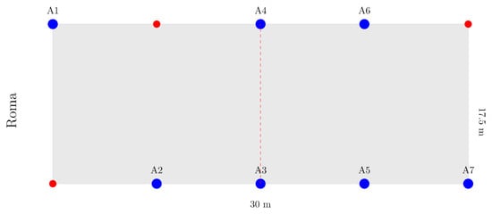
Figure 4.
Experimental monitoring test setup for dynamic measurements on Bridge A.
Frequencies and mode shapes are derived from accelerometric acquisitions recorded during both environmental vibrations and impulsive excitation, generated by the passage of a heavy vehicle over a bump. The two main identified mode shapes are shown in Figure 5 by means of numerical results: these basically involve bending and torsion of the deck, respectively.
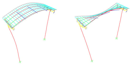
Figure 5.
Mode shapes identified for Bridge A from the experimental dynamic measurements: first flexural mode (left) and first torsional mode (right).
3.2. Bridge B
Bridge B comprises two identical adjacent and connected structures, each featuring an eight-span composite steel–concrete girder deck, for a total of 302 m in length (Figure 6). The outer spans measure 37 m each, while the inner spans are 38 m long. The deck of each of the two structures (Figure 7) consists of two main continuous I-shaped steel beams connected by a series of I-shaped steel cross girders and a 35 cm thick concrete slab, bordered by reinforced concrete curbs. The central curb is used as a connection between the two adjacent decks. The substructure includes seven piers with a composite steel–concrete section and prismatic reinforced concrete abutments.
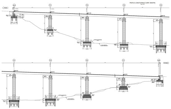
Figure 6.
Longitudinal section of Bridge B (adapted from the original drawing).

Figure 7.
Transverse section of the deck of Bridge B (adapted from the original drawing).
The bridge model is developed in SAP2000 using frame FEs for the steel girders, lateral curbs and piers, and shell FEs for the concrete slab and the central connecting curb (Figure 8). Similarly to Bridge A, all of the dead loads are modeled as equivalent distributed line loads applied to the deck frame FEs, and the connection between the deck and the substructures is modeled with a two-node link system. Additionally, in this case, clamps are applied at the pier bottoms.
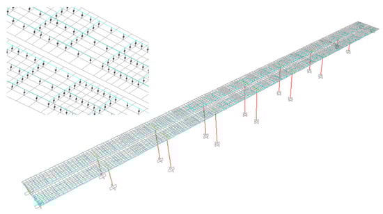
Figure 8.
Finite element model developed for Bridge B, with a focus on the shell mesh.
The monitored points during the experimental measurements are shown in Figure 9. The monitoring system includes mono- and tri-axial MEMS accelerometers, placed on the spans of the bridge according to the two experimental setups of the figure.
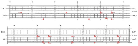
Figure 9.
Experimental monitoring test setup for dynamic measurements on Bridge B.
Frequencies and mode shapes of the bridge are extracted from an operational modal analysis OMA performed recording accelerations under environmental excitation. A total of eight modes are identified; the first two mode shapes are depicted in Figure 10 by means of numerical results, and both mode shapes are basically flexural modes.
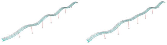
Figure 10.
Mode shapes identified for Bridge B from the experimental dynamic measurements: first flexural (left) and second flexural mode (right).
To be noted is that, in both bridges, although experimental measured points are located on the deck, and despite the simply supported deck configuration of Bridge A, due to the stiffness ratio between the deck and the pier, the modal response of the deck is not vanishingly affected by the stiffness of the piers. For this reason, the inclusion of the piers in the numerical models is essential for the accurate representation of the structure response. This is proven by the coupling in motion shown in Figure 5, for bridge A, and Figure 10 (and even better in the Figure 14 below), for bridge B.
4. Experimental Results
Based on the measured data, the model updating procedure is applied for the two bridges introduced in the previous section, according to the objective functions and sensitivity analyses defined in Section 2.3.
This study primarily focuses on evaluating the role of the objective function, rather than emphasizing the selection of updating parameters. Therefore, for brevity, a single parameter is incorporated within the updating process for each structural model under consideration. Specifically, for Bridge A, the parameter addressed is the Young’s modulus of the concrete utilized in the deck, while for Bridge B, the updating process encompasses the Young’s modulus of the concrete in the deck slab. This methodology, which involves the updating of merely the Young’s modulus, is extensively employed in the literature [30,31], and is also applied for damage detection. It facilitates a focused analysis of the influence of the objective function without the added complexity of adjusting multiple parameters.
Young’s modulus is varied in the range of −20% to +20% of the initial adopted value E0 (E0 = 32.0 GPa for the deck concrete of Bridge A, as indicated by compressive tests on the concrete and by the results of static load tests, and E0 = 34.1 GPa for the slab concrete of Bridge B, as prescribed in the original design). Results of the application of the proposed procedure are presented in the following subsections.
4.1. Bridge A
For Bridge A, since only two modes are available from the experiments, the objective functions (Equations (7)–(12)) are computed by assuming equal (unitary) weights for all modes (). The results of the sensitivity analysis with respect to the deck concrete Young’s modulus are plotted in Figure 11.
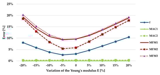
Figure 11.
Percentage errors for the different objective functions adopted in the sensitivity analysis of Bridge A.
Functions f, MFM1, MFM2, and MFM3 provide an optimal value of the parameter equal to a reduction of −5% with respect to the initial guess. By contrast, functions based on MAC seem to be insensitive to the variation, with errors always close to zero. This suggests that the sensitivity of the modal response of bridge A with respect to the selected parameter is higher for the frequencies than mode shapes.
To enhance readability, it is proposed to normalize the sensitivity curves by dividing each one by its maximum value. The results are plotted in Figure 12. This normalization facilitates a more direct and fair comparison between the objective functions, highlighting the differing trends of MAC1 and MAC2, which appear to be not very robust as objective functions. Additionally, it simplifies the identification of the optimal value for the other functions.
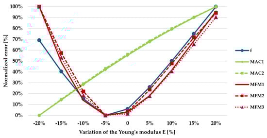
Figure 12.
Normalized percentage errors for the different objective functions adopted in the sensitivity analysis of Bridge A.
For the objective functions f, MFM1, MFM2, and MFM3, Table 2. reports the optimal values of the parameter detectable from the sensitivity curves and the corresponding second-order derivatives, where both the minimum values and the derivatives are computed from the collected discrete points adopting a finite difference scheme [28].
Table 2.
Optimal values of the parameter and relevant second-order derivatives for Bridge A.
All four objective functions have similar derivative values at the minimum, although MFM2 (according to Equation (14)) demonstrates slightly better performance in this regard (shaded row in table). Therefore, selecting any of the four objective functions listed in Table 2 results in minimal differences in the model updating outcomes, confirming the overall stability of the proposed procedure and four functions.
4.2. Bridge B
For Bridge B, where eight vibration modes are identified from OMA, three different approaches for the weighting coefficients are used:
- Case 1: all equal (unitary) weighting coefficients ;
- Case 2: weighting coefficients inversely proportional to the modes order and normalized to obtain a unitary sum ;
- Case 3: weighting coefficients proportional to the OMA power spectral density (PSD) ordinates and normalized to obtain a unitary sum , with being the ordinate of the PSD at the i-th identified frequency.
Figure 13 shows the trends of the six objective functions for Case 2. Similar behaviors are observed for the other two cases. In this figure, to more clearly highlight the differences in the trends of the objective function, the graph is divided into two subplots.
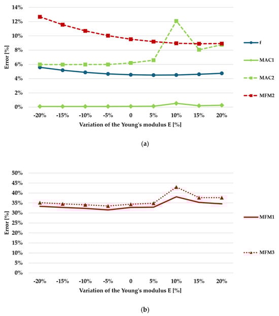
Figure 13.
Percentage errors for the different objective functions adopted in the sensitivity analysis of Bridge B, for Case 2 (i.e., with weighting coefficients proportional to the modes order): (a) objective functions f, MAC1, MAC2, and MFM2; (b) objective functions MFM1 and MFM3.
Functions f and MFM2 exhibit a smooth trend, with a minimum value between +5% and +15% of E0. Function MAC1 appears almost insensitive to the parameter variation, similar to the behavior observed in Bridge A. Consequently, MAC1 is excluded from subsequent analyses. Lastly, functions MAC2, MFM1, and MFM3 display a minimum value around −5% of E0. However, for this bridge, MFM1 and MFM3 indicate a higher overall error level due to the coupling error in frequencies and mode shapes.
It is noteworthy that functions MAC1, MAC2, MFM1, and MFM3, which account for mode shape variation, display a higher total error value for the +10% simulation compared to the rest of the curve. This is due to a coupling in the mode shapes that occurs at a parameter value of 1.1 E0 (+10%). Figure 14 illustrates the deformed shape of one of the vibration modes obtained for (a) E0 (0% variation) and (b) 1.10 E0 (+10% variation). As observed, whereas in the initial model (Figure 14a), this mode shape involves only the flexural vibration of the deck, for 1.10 E0 (Figure 14b) this vibration is coupled with that of one pier. This change in mode shape topology is accurately captured by objective functions MAC1, MAC2, MFM1, and MFM3 but, as expected, is not detected by function f. Function MFM2 also fails to describe this effect, as it is based on the difference in the norm of the modal flexibility matrix (Equation (11)), and thus only captures overall variations in structural behavior.
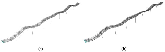
Figure 14.
Deformed shape for the 14th vibration mode of Bridge B obtained for a value of the parameter equal to (a) E0 (0% variation) and (b) 1.10 E0 (+10% variation).
Similarly to Bridge A, the sensitivity curves have been normalized relative to their maximum value to improve readability: Figure 15 shows the normalized sensitivity curves for (a) Case 1, (b) Case 2, and (c) Case 3. As observed for Bridge A, the normalized curve makes the minimum identification easier. It can be observed that:
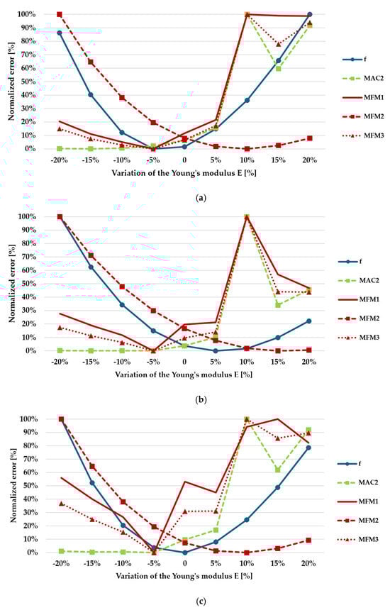
Figure 15.
Normalized percentage errors for the different objective functions adopted in the sensitivity analysis of Bridge B: (a) Case 1 with all equal weighting coefficients; (b) Case 2 with weighting coefficients proportional to the modes order; and (c) Case 3 with weighting coefficients proportional to the PSD ordinates.
- The position of the minimum of function f is sensitive to the weighting scheme; this is located at −5% of E0 for Case 1, at +5% of E0 for Case 2, and at E0 for Case 3;
- The position of the minimum of function MAC2 is insensitive to the weighting scheme, although its identification is not straightforward, due to very small variation for values of the parameter lower than −5% of E0;
- The position of the minimum of functions MFM1 and MFM3 is also insensitive to the weighting scheme, and is located at −5% of E0;
- The position of the minimum of function MFM2 slightly depends on the weighting scheme; this is located at +10% of E0 for Cases 1 and 3, and at +15% of E0 for Case 2.
- As already observed for Figure 13, functions MAC1, MAC2, MFM1, and MFM3 capture the coupling in the mode shapes that occurs at a parameter value of 1.1 E0 (+10%), which results in a peak of the normalized objective function.
Table 3 reports the parameter values at the optimal minimum error and the corresponding second-order derivatives. Functions MFM1 and MFM3 demonstrate the best performance within the set, exhibiting higher values of the second-order derivatives (shaded rows in table). Indeed, as mentioned at the end of Section 2.3, the second-order derivatives represent the local curvature of the function. Hence, higher values indicate that the minimum value can be easily identified, as the objective function is more sloping.
Table 3.
Optimal values of the parameter and relevant second-order derivatives for Bridge B.
5. Conclusions
This study presents a comprehensive examination of dynamic model updating procedures for girder bridge structures, focusing on the influence of different objective functions in improving the alignment between numerical simulations and experimental data. The analysis employs six objective functions, including three novel formulations proposed by the authors and three already widely available in the literature. The considered objective functions involve the numerical and experimental frequencies, the MAC among the relevant mode shapes, and the norm of the corresponding modal flexibility matrices (MFM). The six functions are applied to two real-life case studies: Bridge A, a prestressed RC bridge, and Bridge B, a composite steel–concrete bridge.
Sensitivity analyses were performed by varying the Young’s modulus of the concrete of the deck for Bridge A and of the deck slab for Bridge B. The performance of each objective function in terms of minimizing the discrepancies between the numerical predictions and the experimental data was evaluated, by assuming, as a quantitative selection criterion, the second-order derivative given by the objective function with respect to the varied parameters (Equation (14)). It should be noted that, for the case study of Bridge B (where eight mode shapes are identified), the error given by the function under investigation has been calculated for different types of weighting factors, applied at each addend of the error. They are chosen according to the confidence that the analyst has in the measured data, with the aim of measuring the corresponding importance in the calculations (for Bridge A, where only two modes are identified, only unitary equal coefficients have been considered).
For Bridge A, it was found that the objective functions based on frequencies (f) and MFM (MFM1, MFM2, and MFM3) indicate an optimal value of the parameter around a reduction of −5% on the initial one, showing a general stability of the proposed procedure. On the other hand, functions based on MAC (MAC1 and MAC2) show limited sensitivity to the variation of the stiffness parameter. Therefore, the best choice for objective functions for case study A seems to be between f and MFM, with slight differences in the outcome from one case to another.
In the more complex case study of Bridge B, with eight identified modes, similar trends were observed. Moreover, the inclusion of the mode shapes in the objective functions MAC1, MAC2, MFM1, and MFM3 showed a significant change in the results at specific parameter values, due to the coupling of deck and pier vibrations. Functions MFM1 and MFM3 are also characterized by higher second-order derivative values, and they converge to close minima and optimal values, maintaining stability across different weight types. However, the error evaluated with these two functions is numerically too high (more than 30%, where the objective function f gave an error of around 5%) and therefore misleading with respect to the closeness between numerical and experimental results. Regarding this drawback, the MFM2 function has proven to be more robust, and it is also quasi-stable when the weights are changed, albeit with lower values of the second derivatives.
Overall, this study emphasizes the significance of selecting appropriate objective functions for dynamic model updating. Functions based on frequencies and MFM, especially the MFM2 proposed by the authors, have demonstrated both robustness and effectiveness across case studies. MFM2 is then the suggested method (Equation (11)): this function is sensitive to parameter variations, it is quasi-stable when the weights are varied, and it does not show numerical divergences, although in some instances the identifiability is somewhat not optimal. The result can be seen as a specialization of Ref. [32], another paper where objective functions related to frequency residual only, mode shape residual only, modal flexibility residual only, and their combinations are investigated and compared. The cited work also shows that the introduction of a modal flexibility residual in the objective function considerably improves the detection capability. In this work, an improvement in the definition of the residual has been provided.
These outcomes underscore the potential of advanced objective functions in enhancing the accuracy and reliability of structural models, thereby contributing to more efficient and effective bridge maintenance and management. Further studies on the proposed procedure are expected to generalize the main findings of this paper.
Author Contributions
Conceptualization, P.D.R., I.V. and E.L.; methodology, P.D.R., I.V. and E.L.; software, P.D.R. and I.V.; validation, P.D.R., I.V. and E.L.; formal analysis, I.V.; investigation, P.D.R., I.V. and E.L.; data curation, P.D.R., I.V. and E.L.; writing—original draft preparation, P.D.R., I.V. and E.L.; writing—review and editing, P.D.R., I.V. and E.L.; visualization, P.D.R., I.V. and E.L.; supervision, E.L. All authors have read and agreed to the published version of the manuscript.
Funding
This research received no external funding.
Data Availability Statement
The data presented in this study are available on reasonable request to the corresponding author.
Acknowledgments
P. Di Re acknowledges the research grant SEED PNR 2021—000048 21 SEED DI RE—CUP B89J21032850001 (Sapienza University of Rome). The Authors thank Jacopo Ciambella (Department of Structural and Geotechnical Engineering, Sapienza University of Rome) for his kind support in the acquisition and analysis of the experimental data.
Conflicts of Interest
The authors declare no conflicts of interest.
Nomenclature
| FE | finite element |
| MAC | modal assurance criterion |
| MFM | modal flexibility matrix |
| OMA | operational modal analysis |
| RC | reinforced concrete |
References
- Mottershead, J.E.; Friswell, M.I. Model updating in structural dynamics: A survey. J. Sound Vib. 1993, 167, 347–375. [Google Scholar] [CrossRef]
- Mottershead, J.E.; Link, M.; Friswell, M.I. The sensitivity method in finite element model updating: A tutorial. Mech. Syst. Signal Process. 2011, 25, 2275–2296. [Google Scholar] [CrossRef]
- Simoen, E.; De Roeck, G.; Lombaert, G. Dealing with uncertainty in model updating for damage assessment: A review. Mech. Syst. Signal Process. 2015, 56–57, 123–149. [Google Scholar] [CrossRef]
- Ereiz, S.; Duvnjak, I.; Jiménez-Alonso, J.F. Review of finite element model updating methods for structural applications. Structures 2022, 41, 684–723. [Google Scholar] [CrossRef]
- Reichert, I.; Olney, P.; Lahmer, T. Influence of the error description on model-based design of experiments. Eng. Struct. 2019, 193, 100–109. [Google Scholar] [CrossRef]
- Lofrano, E.; Pingaro, M.; Trovalusci, P.; Paolone, A. Optimal Sensors Placement in Dynamic Damage Detection of Beams Using a Statistical Approach. J. Optim. Theory Appl. 2020, 187, 758–775. [Google Scholar] [CrossRef]
- Di Re, P.; Lofrano, E.; Ciambella, J.; Romeo, F. Structural analysis and health monitoring of twentieth-century cultural heritage: The Flaminio Stadium in Rome. Smart Struct. Syst. 2021, 27, 285–303. [Google Scholar] [CrossRef]
- Xiao, F.; Mao, Y.; Sun, H.; Chen, G.S.; Tian, G. Stiffness Separation Method for Reducing Calculation Time of Truss Structure Damage Identification. Struct. Control Health Monit. 2024, 1, 5171542. [Google Scholar] [CrossRef]
- Xiao, F.; Yan, Y.; Meng, X.; Xu, L.; Chen, G.S. Parameter identification of beam bridges based on stiffness separation method. Structures 2024, 67, 107001. [Google Scholar] [CrossRef]
- Teughels, A.; De Roeck, G. Damage detection and parameter identification by finite element model updating. Rev. Eur. Gen. Civ. 2005, 9, 109–158. [Google Scholar] [CrossRef]
- Schommer, S.; Nguyen, V.H.; Maas, S.; Zürbes, A. Model updating for structural health monitoring using static and dynamic measurements. Proc. Eng. 2017, 199, 2146–2153. [Google Scholar] [CrossRef]
- Mao, Y.; Tian, G.; Chen, G.S. Partial-Model-Based Damage Identification of Long-Span Steel Truss Bridge Based on Stiffness Separation Method. Struct. Control Health Monit. 2024, 1, 5530300. [Google Scholar] [CrossRef]
- Hurtado, O.D.; Ortiz, A.R.; Gomez, D.; Astroza, R. Bayesian Model-Updating Implementation in a Five-Story Building. Buildings 2023, 13, 1568. [Google Scholar] [CrossRef]
- Ruggieri, S.; Bruno, G.; Attolico, A.; Uva, G. Assessing the dredging vibrational effects on surrounding structures: The case of port nourishment in Bari. J. Build. Eng. 2024, 96, 110385. [Google Scholar] [CrossRef]
- Behmanesh, I.; Moaveni, B.; Lombaert, G.; Papadimitriou, C. Hierarchical Bayesian model updating for structural identification. Mech. Syst. Signal Process. 2015, 64–65, 360–376. [Google Scholar] [CrossRef]
- Zhao, H.; Fu, C.; Zhang, Y.; Zhu, W.; Lu, K.; Francis, E.M. Dimensional decomposition-aided metamodels for uncertainty quantification and optimization in engineering: A review. Comput. Methods Appl. Mech. Eng. 2024, 428, 117098. [Google Scholar] [CrossRef]
- Cheng, X.-X. Model Updating for a Continuous Concrete Girder Bridge Using Data from Construction Monitoring. Appl. Sci. 2023, 13, 3422. [Google Scholar] [CrossRef]
- Malekghaini, N.; Ghahari, F.; Ebrahimian, H.; Bowers, M.; Ahlberg, E.; Taciroglu, E. A Two-Step FE Model Updating Approach for System and Damage Identification of Prestressed Bridge Girders. Buildings 2023, 13, 420. [Google Scholar] [CrossRef]
- Liu, C.; Zhang, F.; Ni, Y.; Ai, B.; Zhu, S.; Zhao, Z.; Fu, S. Efficient Model Updating of a Prefabricated Tall Building by a DNN Method. Sensors 2024, 24, 5557. [Google Scholar] [CrossRef]
- Zhao, H.; Lv, J.; Wang, Z.; Gao, T.; Xiong, W. Finite Element Model Updating Using Resonance–Antiresonant Frequencies with Radial Basis Function Neural Network. Appl. Sci. 2023, 13, 6928. [Google Scholar] [CrossRef]
- Cui, J.; Kim, D.; Koo, K.Y.; Chaudhary, S. Structural model updating of steel box girder bridge using modal flexibility based deflections. Balt. J. Road Bridg. Eng. 2012, 7, 253–260. [Google Scholar] [CrossRef]
- Brunetti, M.; Ciambella, J.; Evangelista, L.; Lofrano, E.; Paolone, A.; Vittozzi, A. Experimental results in damping evaluation of a high-speed railway bridge. Procedia Eng. 2017, 199, 3015–3020. [Google Scholar] [CrossRef]
- Gattulli, V.; Lofrano, E.; Paolone, A.; Potenza, F. Measured properties of structural damping in railway bridges. J. Civ. Struct. Health Monit. 2019, 9, 639–653. [Google Scholar] [CrossRef]
- Pastor, M.; Binda, M.; Harcarik, T. Modal Assurance Criterion. Proc. Eng. 2012, 49, 543–548. [Google Scholar] [CrossRef]
- Golub, G.H.; Van Loan, C.F. Matrix Computations, 3rd ed.; Johns Hopkins: Baltimore, MD, USA, 1996. [Google Scholar]
- Jimenez-Alonso, J.F.; Naranjo-Perez, J.; Pavic, A.; Saez, A. Maximum likelihood finite-element model updating of civil engineering structures using nature-inspired computational algorithms. Struct. Eng. Int. 2021, 31, 326–338. [Google Scholar] [CrossRef]
- Di Re, P.; Ciambella, J.; Lofrano, E.; Paolone, A. Dynamic testing and modeling of span interaction in high-speed railway girder bridges. Measurement 2024, 226, 114078. [Google Scholar] [CrossRef]
- Di Re, P.; Benaim Sanchez, D.M. Finite difference technique for the evaluation of the transverse displacements in force-based beam finite elements. Comput. Methods Appl. Mech. Eng. 2024, 428, 117067. [Google Scholar] [CrossRef]
- Computers and Structures Inc. SAP2000 Integrated Software for Structural Analysis and Design; CSI: Berkeley, CA, USA, 2024; Volume 24, Available online: https://www.csiamerica.com/products/sap2000 (accessed on 19 January 2025).
- Aloisio, A.; Pasca, D.P.; Di Battista, L.; Rosso, M.M.; Cucuzza, R.; Marano, G.C.; Alaggio, R. Indirect assessment of concrete resistance from FE model updating and Young’s modulus estimation of a multi-span PSC viaduct: Experimental tests and validation. Structures 2022, 37, 686–697. [Google Scholar] [CrossRef]
- Waeytens, J.; Rosić, B.; Charbonnel, P.E.; Merliot, E.; Siegert, D.; Chapeleau, X.; Vidal, R.; Le Corvec, V.; Cottineau, L.M. Model updating techniques for damage detection in concrete beam using optical fiber strain measurement device. Eng. Struct. 2016, 129, 2–10. [Google Scholar] [CrossRef]
- Jaishi, B.; Ren, W.X. Structural finite element model updating using ambient vibration test results. J. Struct. Eng. 2005, 131, 617–628. [Google Scholar] [CrossRef]
Disclaimer/Publisher’s Note: The statements, opinions and data contained in all publications are solely those of the individual author(s) and contributor(s) and not of MDPI and/or the editor(s). MDPI and/or the editor(s) disclaim responsibility for any injury to people or property resulting from any ideas, methods, instructions or products referred to in the content. |
© 2025 by the authors. Licensee MDPI, Basel, Switzerland. This article is an open access article distributed under the terms and conditions of the Creative Commons Attribution (CC BY) license (https://creativecommons.org/licenses/by/4.0/).