Improving Project Estimates at Completion through Progress-Based Performance Factors

Abstract

From a managerial perspective, project success hinges on estimates at completion as they allow tailoring response actions to cost and schedule overruns. While the literature is moving towards sophisticated approaches, standard methodologies, such as Earned-Value Management (EVM) and Earned Schedule (ES), are barely implemented in certain contexts. Therefore, it is necessary to improve performance forecasting without increasing its difficulty. The objective of this study was twofold. First, to guide modeling and implementing project progress within cost and to schedule Performance Factors (PFs). Second, to test several PFs utilized within EVM and ES formulae to forecast project cost and duration at completion. Progress indicators dynamically adjust the evaluation approach, shifting from neutral to conservative as the project progresses, either physically or temporally. This study compared the performance of the progress-based PFs against EVM and ES standard, combined, and average-based PFs on a dataset of 65 real construction projects, in both cost and duration forecasting. The results show that progress-based PFs provide more accurate, precise, and timely forecasts than other PFs. This study allows practitioners to select one or more of the proposed PFs, or even to develop one, following the guidelines provided, to reflect best their assumptions about the future course of project performance.

1. Introduction

Project monitoring and control processes are crucial to project success. The larger and more complex a project, the higher the likelihood of risks emerging and compromising its performance [1]. Therefore, it is essential to monitor project activities and implement control actions as needed [2].

Control actions are developed based on Estimates at Completion (EACs) obtained from evaluating project performance. The extent of control actions depends on the deviation between the EACs and their corresponding planned values [3]. However, EACs are subject to variability, as various factors influence them, including the interrelationships among project variables [4].

Earned Value Management (EVM) [5] and its extension, Earned Schedule (ES) [6], stand among the most widely adopted project-monitoring methodologies. EVM compares the project Work Performed ($WP$) and the Actual Cost ($AC$) with the Performance Measurement Baseline (PMB), which consists of the Work Scheduled ($WS$) values from the project start and its Planned Duration (PD). In contrast, ES focuses on the homonym metric ($ES$), representing the time when the current $WP$ was scheduled to be attained, as per the PMB.

Previous research has proven EVM and ES effective in multiple projects [7]. However, both methodologies overlook cost and schedule performance relationships and trends [8]. Furthermore, neither EVM nor ES incorporate project progress into the evaluation of EACs. In contrast, the forecasting approach should be contingent on whether the project performance has stabilized [9].

The limitations of EVM and ES have sparked studies exploring alternative methods for project performance forecasting. These studies can be divided into two categories: those that build on and aim to improve EVM and ES and those adopting a different approach, including nonlinear regression, Bayesian inference, and Artificial Intelligence (AI).

Despite the advancements in project-monitoring methodologies, the adoption of EVM and ES remains restricted in specific scenarios [10]. Additionally, the complexity of sophisticated methods poses challenges for practical implementation by practitioners [11]. Consequently, there is a pressing need to enhance project performance forecasting by refining EVM and ES without compromising their simplicity in application.

This study had a twofold objective. First, to guide modeling project progress and implementing it within project Performance Factors (PFs), and to propose a series of progress-based PFs to implement within EVM and ES formulae for evaluating the project cost and duration estimates at completion. Second, to benchmark the proposed progress-based PFs against EVM and ES standard, combined, and average-based PFs under the accuracy, precision, and timeliness criteria at the overall, project, and progress levels.

This paper is structured as follows. Section 1 introduces the background of the study and its objective. Section 2 describes standard and alternative methods to project performance forecasting, highlighting the research gap. Section 3 illustrates the proposed progress modeling, implementation, and benchmarking procedures. Section 4 presents the benchmarking results. Section 5 discusses the results obtained, providing theoretical and practical implications and describing the limitations of the method adopted. Lastly, Section 6 concludes by stating the study limitations and future research avenues.

2. Literature Review

2.1. EVM and ES

EVM assesses project performance, using three metrics: Actual Cost ($AC$), Planned Value ($PV$), and Earned Value ($EV$). Let t indicate time. Following Fleming and Koppelman [12], the $AC$ consists of the actual expenditures incurred by the $WP$, the $PV$ corresponds to the budgeted cost associated with the $WS$, as per

$$PV\left(t\right)=WS\left(t\right)·\mathrm{BAC},$$

(1)

and the $EV$ corresponds to the budgeted cost associated with the $WP$, as per

$$EV\left(t\right)=WP\left(t\right)·\mathrm{BAC}.$$

(2)

EVM evaluates the project Cost Estimate at Completion ($cEAC$) and Time Estimate at Completion ($tEA{C}^{\mathrm{EVM}}$), using two different approaches. The $cEAC$ is determined by the sum of the $AC$ and the cost Estimate-to-Complete ($cETC$) [5], which is evaluated through the ratio of the cost associated with the remaining work ($\mathrm{BAC}-EV$) to the cost Performance Factor ($cPF$), as per

$$cEAC\left(t\right)=AC\left(t\right)+cETC\left(t\right)=AC\left(t\right)+\frac{\mathrm{BAC}-EV\left(t\right)}{cPF\left(t\right)}.$$

(3)

Instead, the $tEA{C}^{\mathrm{EVM}}$ is determined by the ratio of the $\mathrm{PD}$ to the schedule Performance Factor ($sPF$) [5], as per

$$tEA{C}^{\mathrm{EVM}}\left(t\right)=\frac{\mathrm{PD}}{sPF\left(t\right)}.$$

(4)

In standard EVM, the $cPF$ and the $sPF$ are set to the Cost Performance Index ($CPI$) and the Schedule Performance Index ($SP{I}^{\mathrm{EVM}}$), respectively. The former is the ratio of the $EV$ to the $AC$ [5], as per

$$CPI\left(t\right)=\frac{EV\left(t\right)}{AC\left(t\right)},$$

(5)

while the latter is the ratio of the $EV$ to the $PV$ [5], as per

$$SP{I}^{\mathrm{EVM}}\left(t\right)=\frac{EV\left(t\right)}{PV\left(t\right)}.$$

(6)

An index higher, equal, or inferior to 1 indicates performance superior to, on a par with, or below the PMB, respectively.

Previous studies have demonstrated EVM to be effective in cost forecasting [13,14] but not in duration forecasting. Specifically, studies have criticized $SP{I}^{\mathrm{EVM}}$ because it relies on cost metrics (i.e., $EV$ and $PV$), which equal the $\mathrm{BAC}$ of the project’s Actual Duration ($AD$), as per Equations (1) and (2), making the index converge to 1 as the project progresses [15,16]. This limitation has led to exploring alternative methodologies for schedule performance analysis.

ES was developed to overcome the limitations of $SP{I}^{\mathrm{EVM}}$. In ES, schedule performance is based on the $ES$ metric, calculated as per

$$ES\left(t\right)=z+\frac{EV\left(t\right)-PV\left(z\right)}{PV(z+1)-PV\left(z\right)}\mathrm{where}z:PV\left(z\right)\le EV\left(t\right)\le PV(z+1),$$

(7)

assuming linear progress between consecutive $PV$ values [6]. Similar to Equation (3), the ES Time Estimate at Completion ($tEA{C}^{\mathrm{ES}}$) is determined by the sum of t and the Time Estimate to Complete ($tETC$), which consists of the ratio of the “remaining duration” ($\mathrm{PD}-ES$) to the $SP{I}^{\mathrm{ES}}$ [17], as per

$$tEA{C}^{\mathrm{ES}}\left(t\right)=t+tETC\left(t\right)=t+\frac{\mathrm{PD}-ES\left(t\right)}{sPF\left(t\right)}.$$

(8)

In a standard ES, the $sPF$ corresponds to the ES Performance Index ($SP{I}^{\mathrm{ES}}$), which is the ratio of $ES$ to t [6], as per

$$SP{I}^{\mathrm{ES}}\left(t\right)=\frac{ES\left(t\right)}{t}.$$

(9)

Unlike $SP{I}^{\mathrm{EVM}}$, the $SP{I}^{\mathrm{ES}}$ does not converge to 1 as the project approaches completion, remaining meaningful throughout the project duration.

Earlier studies have proven ES more effective than EVM in duration forecasting [18,19]. Nonetheless, both methodologies present further limitations, from assessing cost and schedule performances separately to neglecting trends [20]. These flaws have led researchers to explore alternative methods for project performance forecasting.

Studies on project forecasting methods fall into two categories. The first category entails those studies that rely on standard EVM and ES formulae but implement different PFs. This method prioritizes simplicity as it neither introduces further assumptions nor needs external data. Instead, the second category encompasses those studies that use formulae different from those used by EVM and ES, introducing additional assumptions or relying on external data to improve forecasting performance.

2.2. Performance-Factor-Based Forecasting Methods

PFs can be either time-invariant or time-based. Let x indicate the forecast target. Time-invariant PFs assume the form $xPF=\mathrm{z},\forall t\in [0\dots AD]$. The specific case in which

$$xPF\left(t\right)=\mathrm{z}=1$$

(10)

reflects the assumption by which the current Cost Variance (i.e., $CV=EV-AC$) [5] or the ES Schedule Variance (i.e., $S{V}^{\mathrm{ES}}=ES-t$) [6] will remain the same until project completion (i.e., $cEAC=\mathrm{BAC}-CV$ and $tEA{C}^{\mathrm{ES}}=\mathrm{PD}-S{V}^{\mathrm{ES}}$), whereas setting $sPF=1$ in Equation (4) reflects the assumption by which the project will end exactly on time (i.e., $tEA{C}^{\mathrm{EVM}}=\mathrm{PD}$). In contrast, time-based PFs assume the form $xPF=f[PV,EV,AC,t]$, determining the rate of future accrual ($xPF<1$) or recovery ($xPF>1$) of cost overruns (if $x=c$) or schedule delay (if $x=s$).

Regarding time-based PFs, standard EVM uses the $CPI$ as the $cPF$ and the $SP{I}^{\mathrm{EVM}}$ as the $sPF$. These PFs reflect two assumptions: first, cost and time performances are unrelated, and second, future performance solely depends on the current one, ignoring any trends. To relax these assumptions, studies have proposed combined PFs and average-based PFs.

Combined PFs, combining cost and schedule performances, encompass products and weighted averages of the $cPF$ and the $sPF$. Products include the EVM Critical Ratio ($C{R}^{\mathrm{EVM}}$), as per

$$C{R}^{\mathrm{EVM}}\left(t\right)=CPI\left(t\right)·SP{I}^{\mathrm{EVM}}\left(t\right),$$

(11)

and the ES Critical Ratio ($C{R}^{\mathrm{ES}}$), as per

$$C{R}^{\mathrm{ES}}\left(t\right)=CPI\left(t\right)·SP{I}^{\mathrm{ES}}\left(t\right).$$

(12)

Weighted averages include the EVM Weighted Average ($W{A}^{\mathrm{EVM}}$), as per

$$W{A}^{\mathrm{EVM}}(t;\mathrm{w})=\mathrm{w}·CPI\left(t\right)+(1-\mathrm{w})·SP{I}^{\mathrm{EVM}}\left(t\right),$$

(13)

and the ES Weighted Average ($W{A}^{\mathrm{ES}}$), as per

$$W{A}^{\mathrm{ES}}(t;\mathrm{w})=\mathrm{w}·CPI\left(t\right)+(1-\mathrm{w})·SP{I}^{\mathrm{ES}}\left(t\right),$$

(14)

where w denotes the weight.

Average-based PFs, accounting for past trends in cost and schedule performances, include the cumulative, moving, and exponential moving averages of standard and combined PFs. Let $xPF$ denote the x PF, where $x=c$ indicates cost and $x=s$ indicates schedule. Then, the Cumulative Average (CA) is determined, as per

$$T^{\mathrm{CA}}(xPF,t)=\frac{1}{t}\sum _{j=0}^{t}xPF\left(j\right),$$

(15)

the Moving Average (MA) is determined, as per

$$T^{\mathrm{MA}}(xPF,t;\mathrm{k})=\frac{1}{\mathrm{k}}\sum _{j=t-\mathrm{k}+1}^{t}xPF\left(j\right),$$

(16)

where k indicates the sample window, and the Exponential Moving Average (EMA) is determined, as per

$$T^{\mathrm{EMA}}(xPF,t;\mathsf{\alpha })=\mathsf{\alpha }·xPF\left(t\right)+(1-\mathsf{\alpha })·T^{\mathrm{EMA}}(xPF,t-1;\mathsf{\alpha }),$$

(17)

where $\mathsf{\alpha }$ indicates the smoothing factor, and $0\le \mathsf{\alpha }\le 1$.

Combined PFs have been tested in cost forecasting [13,21,22,23,24,25] and duration forecasting [18,26,27]. The same applies to the Cumulative Average and the Moving Average [22,28,29], as well as to the Exponential Moving Average [30,31,32]. In all the studies above, while the best PF depended on the specific project characteristics, the $CPI$ and the $SP{I}^{\mathrm{ES}}$ were proven the most robust.

2.3. Other Forecasting Methods

Alternative forecasting methods to improve performance forecasting offer more sophisticated modeling capabilities, but they come at the expense of increased difficulty in implementation. The methods include nonlinear regression, Bayesian inference, and AI.

Nonlinear regression studies are based on the properties of project S-curves. Specifically, the studies calculate duration and cost estimates at completion by fitting theoretical models to the $EV$ and $AC$ data, respectively, and projecting the resulting models forward. The method was tested in both cost forecasting [33,34] and duration forecasting [35,36]. The difficulties related to nonlinear regression lie in choosing the theoretical model and performing the curve-fitting procedure.

Bayesian inference methods rely on external data to evaluate the parameters of ex-ante distributions [37] and use internal project-monitoring data to refine such distributions during project execution. These methods are applied to project S-curves [38], to cost- and schedule-overruns probability [39], and to risks-occurrences probability [40]. In adopting the Bayesian approach, the difficulties lie in defining the ex-ante distributions, collecting data to evaluate their parameters, and updating the parameters with the project in place.

AI algorithms use external data to build project-cost and duration forecasting models. Several reviews of AI applications in project monitoring are available, including [41,42,43]. Algorithms include linear regression [44], support vector machine [45,46,47], tree-based methods [48,49], k-nearest neighbors [50], ensemble methods [51,52], and artificial neural networks [53,54,55,56,57,58,59]. The difficulty in using AI models lies in collecting the data and in the procedures required to prevent underfitting and overfitting.

2.4. Research Gap

Despite the potential improvements in forecasting performance, alternative methods to EVM and ES are rarely utilized in practice. This is due to several factors, chief among them being difficulty in implementation or, one step earlier, lack of data on which to base the necessary assumptions. For this reason, where the preconditions for adopting more sophisticated methods are lacking, practitioners need simple methods that do not deviate excessively from standard EVM and ES. In light of this, this study provides progress-based PFs to predict the project-cost and duration estimates at completion while maximizing the trade-off between prediction performance and implementation difficulty. All PFs consider the current state of progress, which is used to move from a conservative projection to a bottom-up projection as the project approaches completion.

3. Research Methodology

This section is divided into two parts. The first part introduces the PFs that will be tested and describes how to model and implement progress within them. The second part describes the benchmarking, including the procedures to preprocess the data and the criteria to evaluate the forecasting performance of the models implementing the PFs.

3.1. Progress-Based Performance Factors

This study tested four categories of PFs: standard, combined, average-based, and progress-based. Standard PFs include EVM and ES indexes. Combined PFs include combinations of standard PFs. Average-based PFs are evaluated by calculating different types of averages of standard and combined PFs. Lastly, progress-based PFs are evaluated by modeling and implementing progress within standard PFs.

Let $PI$ denote the generic Progress Indicator. Then, $PI$ should be expressed in terms of physical or time progress, and $\left|PI\right|$ should range between 0% and 100% (i.e., $0\le \left|PI\right|\le 1$). In light of this, physical progress can be expressed as per $WP=EV/\mathrm{BAC}$ while time progress can be expressed as per $E{S}_{\mathrm{s}}=ES/\mathrm{PD}$, where the subscript “s” distinguishes the scaled from the unscaled variable.

This study sought to integrate $PI$ into the $xETC$ calculation, to shift from a neutral approach ($xPF=1$) to a more conservative one ($xPF\ne 1$) as project performance stabilized. Since $0\le \left|PI\right|\le 1$, $PI$ could be implemented as a weight ($P_w$) or an exponent ($P_x$). When implemented as a weight, $T^{\mathrm{WAP}}$ was determined, as per

$$T^{\mathrm{WAP}}(xPF,P{I}_w,t)=[1-P{I}_w\left(t\right)]·1+P_w\left(t\right)·xPF\left(t\right).$$

(18)

While $P{I}_w=0$ determined $T^{\mathrm{WAP}}=1$, $P{I}_w=1$ determined $T^{\mathrm{WAP}}=xPF$. When implemented as an exponent, $T^{\mathrm{XP}}$ was determined, as per

$$T^{\mathrm{XP}}(xPF,P{I}_x,t)={xPF\left(t\right)}^{\pm P{I}_x\left(t\right)}.$$

(19)

The effect of $\pm P{I}_x$ on $T^{\mathrm{XP}}$ was determined by both the $P{I}_x$ sign and the value of $xPF$, as per Table 1.

Table 1. Combinations of $P{I}_x$ and $xPF$ and their effect on $T^{\mathrm{XP}}$.

Scenario	$\mathit{xPF}$
	<1	=1	>1
$P{I}_x=-1$	$T^{\mathrm{XP}}>xPF$	$T^{\mathrm{XP}}=1$	$T^{\mathrm{XP}}<xPF$
$-1<P{I}_x<0$	$T^{\mathrm{XP}}>xPF$	$T^{\mathrm{XP}}=1$	$T^{\mathrm{XP}}<xPF$
$P{I}_x=0$	$T^{\mathrm{XP}}=1$	$T^{\mathrm{XP}}=1$	$T^{\mathrm{XP}}=1$
$0<P{I}_x<1$	$T^{\mathrm{XP}}>xPF$	$T^{\mathrm{XP}}=1$	$T^{\mathrm{XP}}<xPF$
$P{I}_x=1$	$T^{\mathrm{XP}}=xPF$	$T^{\mathrm{XP}}=1$	$T^{\mathrm{XP}}=xPF$

The generic progress-based PFs could be evaluated by combining Equations (18) and (19) into

$$\begin{array}{c}\hfill T^{\mathrm{WAXP}}(xPF,P{I}_w,P{I}_x,t)=[1-P{I}_w\left(t\right)]·1+P{I}_w\left(t\right)·{xPF\left(t\right)}^{\pm P{I}_x\left(t\right)}.\end{array}$$

(20)

The combinations of $P{I}_w$ and $P{I}_x$ determined the pace at which $T^{\mathrm{WAXP}}$ shifted from neutral to conservative.

To summarize, the standard PFs included 1, $CPI$, $SP{I}^{\mathrm{EVM}}$, and $SP{I}^{\mathrm{ES}}$. The combined PFs included $C{R}^{\mathrm{EVM}}$, $C{R}^{\mathrm{ES}}$, $W{A}^{\mathrm{EVM}}$, and $W{A}^{\mathrm{ES}}$. The average-based PFs were evaluated using all the standard PFs but 1 and the combined PFs; the parameters k and $\mathsf{\alpha }$ were set only once. The progress-based PFs were evaluated using all the standard PFs but 1, and all the possible combinations of $+WP$, $-WP$, $E{S}_{\mathrm{s}}$, and $-E{S}_{\mathrm{s}}$ as $P{I}_x$ and $P{I}_w$. The total number of PFs amounted to 71; the complete list will be provided when presenting the benchmarking results.

3.2. Benchmarking

Benchmarking PFs involves testing them in cost and duration forecasting on a real project dataset. This phase entails five steps: Data Collection, Scaling, Interpolation, Forecasts Evaluation, and Performance Assessment.

3.2.1. Data Collection

Data Collection involves retrieving monitoring data from real projects to develop the testing dataset. This study used 65 projects selected from the Operations Research and Scheduling Research group of the Faculty of Economics and Business Administration at Ghent University (Belgium) database [60]. Selection criteria ensured projects experienced both cost and schedule variances throughout their execution. Table 2 provides the projects’ building type, the number of activities in the network, $\mathrm{BAC}$, $\mathrm{PD}$, $AC\left(AD\right)$, and $AD$.

Table 2. Projects properties.

Code	Building Type	#Activities	$\mathbf{BAC}$	$\mathbf{PD}$	$\mathit{AC}\left(\mathit{AD}\right)$	$\mathit{AD}$
C2011-10	Residential	32	484,398.41	39	494,947.71	41
C2011-12	Commercial	49	3,027,133.19	7	3,102,395.91	7
C2011-13	Industrial	134	21,369,835.51	105	26,077,764.74	120
C2012-13	Civil	74	336,410.15	25	350,511.31	28
C2012-17	Residential	33	241,015.00	29	314,856.14	41
C2013-01	Civil	42	1,069,532.42	6	1,314,584.58	6
C2013-02	Civil	181	1,236,603.66	17	1,146,444.38	17
C2013-03	Institutional	55	15,440,865.89	18	16,338,027.20	18
C2013-04	Institutional	252	2,113,684.00	7	2,512,524.00	11
C2013-06	Institutional	276	19,429,810.51	19	21,546,846.18	18
C2013-07	Residential	46	180,476.47	10	175,030.65	11
C2013-08	Residential	42	501,029.51	10	576,624.05	13
C2013-09	Commercial	71	1,537,398.51	8	1,696,971.79	10
C2013-10	Civil	197	11,421,890.36	30	15,218,926.38	30
C2013-11	Civil	167	5,480,518.91	21	5,451,028.00	20
C2013-12	Institutional	27	818,439.99	3	879,853.17	5
C2013-13	Commercial	11	1,118,496.59	10	955,929.22	9
C2013-14	Commercial	9	85,847.89	2	75,468.30	2
C2013-15	Commercial	17	341,468.11	5	298,833.81	4
C2013-16	Commercial	7	248,203.92	6	198,567.00	5
C2013-17	Commercial	23	244,205.40	6	203,605.97	5
C2014-01	Residential	52	38,697,822.73	24	39,777,643.30	23
C2014-04	Industrial	24	62,385,597.58	24	65,526,930.04	36
C2014-05	Residential	25	532,410.29	11	591,410.53	13
C2014-06	Residential	29	3,486,375.47	17	3,599,114.11	19
C2014-07	Residential	25	1,102,536.78	12	1,289,696.78	14
C2014-08	Residential	39	1,992,222.09	11	2,380,299.86	13
C2015-01	Institutional	27	612,769.44	6	646,473.65	9
C2015-02	Civil	216	1,121,316.94	8	967,988.79	9
C2015-03	Industrial	135	2,244,090.74	9	1,868,796.28	10
C2015-04	Residential	56	2,750,938.00	7	2,590,796.73	8
C2015-05	Residential	64	2,524,765.19	4	2,563,675.86	5
C2015-06	Residential	184	143,673.20	9	186,107.00	10
C2015-07	Industrial	138	5,999,600.00	8	5,414,544.00	9
C2015-08	Commercial	186	467,297.21	8	461,900.17	8
C2015-09	Civil	348	1,457,424.00	6	2,145,682.26	9
C2015-27	Civil	18	22,703.52	5	25,313.12	6
C2015-29	Institutional	204	1,874,496.82	8	1,887,087.25	8
C2015-30	Residential	40	440,940.89	14	440,940.89	14
C2015-31	Residential	29	1,310,723.46	16	1,282,185.98	21
C2015-32	Residential	53	2,509,031.42	15	2,509,031.42	14
C2015-33	Civil	12	214,417.71	3	224,789.67	5
C2015-34	Civil	13	511,325.86	4	440,394.16	7
C2015-35	Residential	10	14,956,314.25	38	16,068,878.30	41
C2016-01	Civil	28	671,383.50	12	703,703.50	14
C2016-02	Civil	23	962,181.56	12	972,341.56	13
C2016-03	Civil	25	926,888.01	10	910,728.01	11
C2016-07	Commercial	110	930,179.09	8	932,757.25	11
C2016-11	Residential	55	162,472.00	5	163,189.00	5
C2016-12	Residential	59	222,858.00	5	226,285.00	5
C2016-13	Residential	51	367,952.00	4	379,300.00	5
C2016-14	Residential	48	218,366.00	5	222,021.78	5
C2016-15	Residential	13	95,694.00	4	100,763.00	4
C2016-27	Residential	16	813,663.06	3	879,701.06	4
C2016-28	Residential	19	569,177.85	4	586,086.85	4
C2016-29	Residential	19	1,797,873.62	4	1,860,330.62	4
C2016-30	Residential	23	1,319,736.29	3	1,353,361.29	4
C2016-31	Residential	23	488,936.00	3	498,473.00	4
C2016-32	Residential	22	477,381.00	4	496,991.00	4
C2016-33	Residential	23	377,282.00	3	394,829.00	4
C2016-34	Residential	23	362,476.00	3	383,871.00	3
C2019-01	Residential	86	1,292,979.00	8	1,315,819.86	10
C2019-02	Residential	18	734,602.11	9	748,555.80	9
C2019-03	Civil	17	967,878.00	20	1,270,875.82	22
C2019-04	Civil	33	4,318,950.00	18	4,232,553.41	24

3.2.2. Data Scaling

Data scaling involves expressing project data on a unitless scale. This step prevented projects with metrics expressed in different orders of magnitude from biasing the performance scores. Scaling was achieved by dividing the cost metrics (i.e., $PV$, $EV$, and $AC$) by the $\mathrm{BAC}$ and time metrics (i.e., t, $ES$) by the $\mathrm{PD}$. All the scaled metrics but $WP$ and $WS$ were denoted using the subscript “s”. All the scaled metrics but t, $AD$, and $AC$ ranged between 0 and 1.

3.2.3. Data Interpolation

Data interpolation involves evaluating the project metrics at specific points in time. This step allowed inferring the project’s evolution through all its stages. Interpolation was performed linearly to obtain the project metrics values at 5% progress intervals (i.e., $WP=.05,.10,\dots ,.95$. Records corresponding to $WP=0$ and $WP=1$ were omitted as no forecasts were calculated at the project start (i.e., $WP=0$) and end (i.e., $WP=1$).

3.2.4. Forecast Evaluation

Forecast Evaluation involves using the PFs to calculate the project estimates at completion. All 71 PFs were used for both cost and duration forecasting. Cost forecasts were determined by implementing the PFs as the $cPF$ within Equation (3), while duration forecasts were determined by implementing the PFs as the $sPF$ within Equation (8).

3.2.5. Performance Assessment

This study compared the PFs’ forecasting performance under three criteria: accuracy, precision, and timeliness. Accuracy referred to the ability to provide forecasts close to the real value of the target variable. Precision referred to the ability to minimize the dispersion of forecast errors. Timeliness referred to how fast forecasts achieved accuracy and precision.

For each observation i in the dataset, we let $y_i$ and ${\widehat{y}}_i$ indicate the real value and the forecast for that observation, respectively. Then, the forecast error ($E_i$) was determined by the difference between $y_i$ and ${\widehat{y}}_i$, as per

$$E_i=y_i-{\widehat{y}}_i$$

(21)

All performance criteria could be assessed by analyzing the functional boxplots of the forecast errors. In the functional-boxplot variant, all measures were expressed as a function of the $WP$. The variables $Q_1$, $Q_2$, and $Q_3$ represented the first, second, and third quartiles, respectively, while $LB$ indicated the lower bound and $UB$ the upper bound. Unlike in standard boxplots, this study defined the $LB$ and the $UB$ as the 10th and 90th percentiles of $E_i$, respectively.

Figure 1 illustrates a functional boxplot with the $WP$ on the x-axis. The filled area between $Q_3$ and $Q_1$ represents the functional InterQuartile Range ($IQR=Q_3-Q_1$). Following this notation, accuracy was assessed based on how close $Q_1$, $Q_2$, and $Q_3$ fall to the $WP$ axis (i.e., $E=0$), precision was assessed by the extent of the areas between the $UB$ and the $LB$ and the $IQR$, and timeliness was determined by how fast these measures converged.

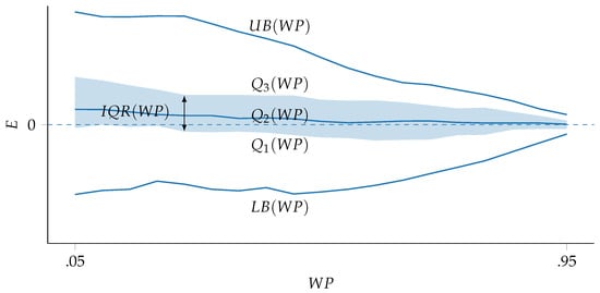
Figure 1. Example of forecast Error (E) functional boxplot with the Work Performed ($WP$) as the x-axis.

All performance criteria but timeliness could be summarized at a higher level without analyzing each PF functional boxplot. To achieve this, the benchmark utilized three regression scores: Mean Absolute Error ($MAE$), measuring average accuracy, Root Mean Squared Error ($RMSE$), measuring robustness, and a custom score based on the area determined by $Q_1$ and $Q_3$ throughout the project progress (A), measuring precision.

We let n indicate the total number of observations in the project dataset. Then, the $MAE$ was evaluated, as per

$$MAE=\frac{1}{n}\sum _{i=0}^n\left|E_i\right|,$$

(22)

the $RMSE$ was evaluated, as per

$$RMSE=\sqrt{\frac{1}{n}\sum _{i=0}^n{\left(E_i\right)}^2},$$

(23)

and A was calculated by evaluating the integral between the first and third quartiles lines and the $WP$-axis ($E_i=0$), as per

$$A=A_{Q_1,0}+A_{Q_3,0}={\int }_{WP=.5}^{.95}\left|Q_1\left(WP\right)\right|\mathrm{d}WP+{\int }_{WP=.5}^{.95}\left|Q_3\left(WP\right)\right|\mathrm{d}WP.$$

(24)

Figure 2 provides an example of how A was calculated. The light blue area corresponds to $A_{Q_3,0}$, while the dark blue one corresponds to $A_{Q_1,0}$.

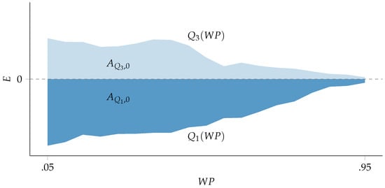
Figure 2. Example of functional boxplot Area score (A) evaluation.

4. Results

The PF parameters were assigned arbitrary values: weight parameter $\mathrm{w}=0.8$, sample window parameter $\mathrm{k}=1/10\mathrm{PD}$, and smoothing parameter $\mathsf{\alpha }=0.75$.

Table 3 presents the A, rank, $MAE$, and $RMSE$ scores of the $cPF$s, calculated on the entire dataset. The rank was determined based on the ascending order of A. The best-performing PF was $T^{\mathrm{XP}}(CPI,WP)$, ranking first with $MAE=0.0624$ and $RMSE=0.1220$. Among non-progress-based PFs, 1 ranked highest, placing 12th with $MAE=0.0638$ and $RMSE=0.1132$. The best-performing standard PF was $CPI$, ranking 37th with $MAE=0.0793$ and $RMSE=0.1662$.

Table 3. Cost PFs forecasts: overall accuracy scores.

$\mathit{cPF}$	Rank	A	$\mathit{MAE}$	$\mathit{RMSE}$
$T^{\mathrm{XP}}(CPI,WP)$	1	0.8667	0.0624	0.1220
$T^{\mathrm{WAXP}}(CPI,E{S}_{\mathrm{s}},E{S}_{\mathrm{s}})$	2	0.8758	0.0611	0.1130
$T^{\mathrm{WAP}}(CPI,WP)$	3	0.8911	0.0628	0.1241
$T^{\mathrm{WAXP}}(CPI,WP,WP)$	4	0.8931	0.0622	0.1170
$T^{\mathrm{WAXP}}(CPI,E{S}_{\mathrm{s}},WP)$	5	0.8962	0.0617	0.1149
$T^{\mathrm{WAXP}}(CPI,WP,E{S}_{\mathrm{s}})$	6	0.8980	0.0617	0.1147
$T^{\mathrm{WAP}}(CPI,E{S}_{\mathrm{s}})$	7	0.9063	0.0623	0.1200
$T^{\mathrm{XP}}(CPI,E{S}_{\mathrm{s}})$	8	0.9096	0.0623	0.1190
$T^{\mathrm{WAXP}}(SP{I}^{\mathrm{ES}},E{S}_{\mathrm{s}},E{S}_{\mathrm{s}})$	9	0.9675	0.0626	0.1103
$T^{\mathrm{WAXP}}(SP{I}^{\mathrm{ES}},E{S}_{\mathrm{s}},WP)$	10	0.9884	0.0638	0.1121
$T^{\mathrm{WAXP}}(SP{I}^{\mathrm{ES}},WP,E{S}_{\mathrm{s}})$	11	0.9994	0.0640	0.1125
1	12	1.0270	0.0638	0.1132
$T^{\mathrm{WAXP}}(SP{I}^{\mathrm{EVM}},E{S}_{\mathrm{s}},WP)$	13	1.0304	0.0616	0.1091
$T^{\mathrm{WAXP}}(SP{I}^{\mathrm{ES}},WP,WP)$	14	1.0693	0.0655	0.1150
$T^{\mathrm{WAXP}}(SP{I}^{\mathrm{EVM}},WP,WP)$	15	1.0724	0.0625	0.1109
$T^{\mathrm{WAXP}}(SP{I}^{\mathrm{EVM}},WP,E{S}_{\mathrm{s}})$	16	1.0765	0.0622	0.1098
$T^{\mathrm{WAXP}}(CPI,WP,-WP)$	17	1.0879	0.0663	0.1110
$T^{\mathrm{WAXP}}(CPI,E{S}_{\mathrm{s}},-WP)$	18	1.1166	0.0668	0.1136
$T^{\mathrm{WAXP}}(CPI,WP,-E{S}_{\mathrm{s}})$	19	1.1171	0.0668	0.1135
$T^{\mathrm{WAXP}}(SP{I}^{\mathrm{ES}},WP,-WP)$	20	1.1435	0.0726	0.1199
$T^{\mathrm{WAXP}}(CPI,E{S}_{\mathrm{s}},-E{S}_{\mathrm{s}})$	21	1.1459	0.0680	0.1174
$T^{\mathrm{XP}}(CPI,-WP)$	22	1.1597	0.0682	0.1093
$T^{\mathrm{WAXP}}(SP{I}^{\mathrm{EVM}},E{S}_{\mathrm{s}},E{S}_{\mathrm{s}})$	23	1.1761	0.0658	0.1139
$T^{\mathrm{CA}}\left(CPI\right)$	24	1.1844	0.0779	0.1543
$T^{\mathrm{CA}}\left(W{A}^{\mathrm{ES}}\right)$	25	1.1847	0.0757	0.1456
$T^{\mathrm{WAXP}}(SP{I}^{\mathrm{ES}},E{S}_{\mathrm{s}},-WP)$	26	1.1853	0.0728	0.1198
$T^{\mathrm{WAXP}}(SP{I}^{\mathrm{EVM}},WP,-WP)$	27	1.1872	0.0768	0.1260
$T^{\mathrm{WAXP}}(SP{I}^{\mathrm{ES}},WP,-E{S}_{\mathrm{s}})$	28	1.1974	0.0728	0.1200
$T^{\mathrm{MA}}\left(W{A}^{\mathrm{ES}}\right)$	29	1.2201	0.0764	0.1496
$T^{\mathrm{MA}}\left(CPI\right)$	30	1.2242	0.0776	0.1577
$T^{\mathrm{EMA}}\left(W{A}^{\mathrm{ES}}\right)$	31	1.2286	0.0774	0.1526
$W{A}^{\mathrm{ES}}$	32	1.2332	0.0786	0.1554
$T^{\mathrm{EMA}}\left(CPI\right)$	33	1.2384	0.0782	0.1617
$T^{\mathrm{XP}}(CPI,-E{S}_{\mathrm{s}})$	34	1.2388	0.0711	0.1182
$T^{\mathrm{EMA}}\left(W{A}^{\mathrm{EVM}}\right)$	35	1.2458	0.0801	0.1601
$W{A}^{\mathrm{EVM}}$	36	1.2461	0.0811	0.1626
$CPI$	37	1.2495	0.0793	0.1662
$T^{\mathrm{MA}}\left(W{A}^{\mathrm{EVM}}\right)$	38	1.2537	0.0797	0.1578
$T^{\mathrm{WAP}}(SP{I}^{\mathrm{ES}},WP)$	39	1.2711	0.0719	0.1216
$T^{\mathrm{CA}}\left(W{A}^{\mathrm{EVM}}\right)$	40	1.3000	0.0810	0.1561
$T^{\mathrm{WAXP}}(SP{I}^{\mathrm{ES}},E{S}_{\mathrm{s}},-E{S}_{\mathrm{s}})$	41	1.3084	0.0746	0.1228
$T^{\mathrm{WAP}}(SP{I}^{\mathrm{EVM}},WP)$	42	1.3504	0.0731	0.1245
$T^{\mathrm{WAXP}}(SP{I}^{\mathrm{EVM}},E{S}_{\mathrm{s}},-WP)$	43	1.3565	0.0791	0.1301
$T^{\mathrm{WAP}}(SP{I}^{\mathrm{ES}},E{S}_{\mathrm{s}})$	44	1.3580	0.0687	0.1149
$T^{\mathrm{XP}}(SP{I}^{\mathrm{ES}},WP)$	45	1.3617	0.0772	0.1343
$T^{\mathrm{WAXP}}(SP{I}^{\mathrm{EVM}},WP,-E{S}_{\mathrm{s}})$	46	1.3652	0.0794	0.1308
$T^{\mathrm{XP}}(SP{I}^{\mathrm{ES}},E{S}_{\mathrm{s}})$	47	1.3674	0.0712	0.1194
$T^{\mathrm{WAXP}}(SP{I}^{\mathrm{EVM}},E{S}_{\mathrm{s}},-E{S}_{\mathrm{s}})$	48	1.4126	0.0851	0.1443
$T^{\mathrm{XP}}(SP{I}^{\mathrm{EVM}},WP)$	49	1.4147	0.0726	0.1215
$T^{\mathrm{WAP}}(SP{I}^{\mathrm{EVM}},E{S}_{\mathrm{s}})$	50	1.5436	0.0796	0.1366
$T^{\mathrm{XP}}(SP{I}^{\mathrm{ES}},-E{S}_{\mathrm{s}})$	51	1.5685	0.0866	0.1362
$T^{\mathrm{XP}}(SP{I}^{\mathrm{ES}},-WP)$	52	1.5810	0.0856	0.1337
$T^{\mathrm{XP}}(SP{I}^{\mathrm{EVM}},-WP)$	53	1.6351	0.0978	0.1612
$T^{\mathrm{XP}}(SP{I}^{\mathrm{EVM}},E{S}_{\mathrm{s}})$	54	1.6569	0.0836	0.1468
$T^{\mathrm{XP}}(SP{I}^{\mathrm{EVM}},-E{S}_{\mathrm{s}})$	55	1.7554	0.1116	0.2235
$T^{\mathrm{CA}}\left(SP{I}^{\mathrm{ES}}\right)$	56	3.4251	0.1445	0.2643
$T^{\mathrm{CA}}\left(C{R}^{\mathrm{ES}}\right)$	57	3.4344	0.1670	0.2929
$T^{\mathrm{MA}}\left(SP{I}^{\mathrm{ES}}\right)$	58	3.4371	0.1606	0.3470
$T^{\mathrm{EMA}}\left(SP{I}^{\mathrm{ES}}\right)$	59	3.5705	0.1743	0.3915
$T^{\mathrm{CA}}\left(SP{I}^{\mathrm{EVM}}\right)$	60	3.5828	0.1592	0.2576
$SP{I}^{\mathrm{ES}}$	61	3.6529	0.1930	0.5223
$T^{\mathrm{MA}}\left(C{R}^{\mathrm{ES}}\right)$	62	3.7078	0.1936	0.3866
$T^{\mathrm{MA}}\left(SP{I}^{\mathrm{EVM}}\right)$	63	3.8219	0.1735	0.3089
$T^{\mathrm{EMA}}\left(SP{I}^{\mathrm{EVM}}\right)$	64	4.0941	0.1887	0.3603
$T^{\mathrm{EMA}}\left(C{R}^{\mathrm{ES}}\right)$	65	4.1227	0.2116	0.4370
$T^{\mathrm{CA}}\left(C{R}^{\mathrm{EVM}}\right)$	66	4.2254	0.1900	0.2973
$SP{I}^{\mathrm{EVM}}$	67	4.2499	0.2106	0.5122
$C{R}^{\mathrm{ES}}$	68	4.2571	0.2322	0.5552
$T^{\mathrm{MA}}\left(C{R}^{\mathrm{EVM}}\right)$	69	4.6078	0.2144	0.3732
$T^{\mathrm{EMA}}\left(C{R}^{\mathrm{EVM}}\right)$	70	4.8626	0.2346	0.4331
$C{R}^{\mathrm{EVM}}$	71	4.9789	0.2599	0.5708

Table 4 presents the A, rank, $MAE$, and $RMSE$ scores of the $sPF$s, calculated on the entire dataset. The rank was determined based on the ascending order of A. The best-performing PF was $T^{\mathrm{WAXP}}(CPI,E{S}_{\mathrm{s}},WP)$, ranking first with $MAE=0.1158$ and $RMSE=0.1645$. Among the non-progress-based PFs, 1 ranked highest, placing 6th with $MAE=0.1180$ and $RMSE=0.1670$. The best-performing standard PF was $CPI$, ranking 49th with $MAE=0.1284$ and $RMSE=0.1811$.

Table 4. Schedule PFs forecasts: overall accuracy scores.

$\mathit{sPF}$	Rank	A	$\mathit{MAE}$	$\mathit{RMSE}$
$T^{\mathrm{WAXP}}(CPI,E{S}_{\mathrm{s}},WP)$	1	3.1647	0.1158	0.1645
$T^{\mathrm{WAXP}}(CPI,WP,E{S}_{\mathrm{s}})$	2	3.1652	0.1159	0.1645
$T^{\mathrm{WAXP}}(CPI,E{S}_{\mathrm{s}},E{S}_{\mathrm{s}})$	3	3.1663	0.1159	0.1645
$T^{\mathrm{WAXP}}(CPI,WP,WP)$	4	3.1705	0.1159	0.1646
$T^{\mathrm{WAXP}}(SP{I}^{\mathrm{ES}},E{S}_{\mathrm{s}},E{S}_{\mathrm{s}})$	5	3.1872	0.1210	0.1683
1	6	3.2053	0.1180	0.1670
$T^{\mathrm{WAP}}(CPI,WP)$	7	3.2083	0.1172	0.1645
$T^{\mathrm{XP}}(CPI,WP)$	8	3.2165	0.1166	0.1639
$T^{\mathrm{WAXP}}(SP{I}^{\mathrm{ES}},WP,E{S}_{\mathrm{s}})$	9	3.2215	0.1225	0.1707
$T^{\mathrm{WAXP}}(SP{I}^{\mathrm{ES}},E{S}_{\mathrm{s}},WP)$	10	3.2223	0.1222	0.1701
$T^{\mathrm{XP}}(CPI,E{S}_{\mathrm{s}})$	11	3.2225	0.1163	0.1633
$T^{\mathrm{WAP}}(CPI,E{S}_{\mathrm{s}})$	12	3.2298	0.1166	0.1636
$T^{\mathrm{WAXP}}(SP{I}^{\mathrm{EVM}},WP,E{S}_{\mathrm{s}})$	13	3.2410	0.1216	0.1682
$T^{\mathrm{WAXP}}(SP{I}^{\mathrm{EVM}},WP,WP)$	14	3.2416	0.1226	0.1693
$T^{\mathrm{WAXP}}(SP{I}^{\mathrm{EVM}},E{S}_{\mathrm{s}},WP)$	15	3.2449	0.1215	0.1680
$T^{\mathrm{WAXP}}(SP{I}^{\mathrm{ES}},WP,-WP)$	16	3.2618	0.1206	0.1716
$T^{\mathrm{XP}}(SP{I}^{\mathrm{ES}},E{S}_{\mathrm{s}})$	17	3.2680	0.1269	0.1745
$T^{\mathrm{WAXP}}(CPI,E{S}_{\mathrm{s}},-E{S}_{\mathrm{s}})$	18	3.2737	0.1218	0.1706
$T^{\mathrm{WAP}}(SP{I}^{\mathrm{ES}},E{S}_{\mathrm{s}})$	19	3.2903	0.1258	0.1721
$T^{\mathrm{WAXP}}(CPI,WP,-E{S}_{\mathrm{s}})$	20	3.2921	0.1218	0.1708
$T^{\mathrm{WAXP}}(CPI,E{S}_{\mathrm{s}},-WP)$	21	3.2926	0.1218	0.1707
$T^{\mathrm{WAXP}}(SP{I}^{\mathrm{ES}},WP,WP)$	22	3.3066	0.1253	0.1748
$T^{\mathrm{WAXP}}(CPI,WP,-WP)$	23	3.3071	0.1226	0.1718
$T^{\mathrm{WAXP}}(SP{I}^{\mathrm{ES}},E{S}_{\mathrm{s}},-WP)$	24	3.3189	0.1198	0.1698
$T^{\mathrm{WAXP}}(SP{I}^{\mathrm{EVM}},E{S}_{\mathrm{s}},E{S}_{\mathrm{s}})$	25	3.3217	0.1223	0.1687
$T^{\mathrm{WAXP}}(SP{I}^{\mathrm{ES}},WP,-E{S}_{\mathrm{s}})$	26	3.3230	0.1197	0.1697
$T^{\mathrm{WAXP}}(SP{I}^{\mathrm{ES}},E{S}_{\mathrm{s}},-E{S}_{\mathrm{s}})$	27	3.4070	0.1202	0.1702
$T^{\mathrm{XP}}(SP{I}^{\mathrm{ES}},WP)$	28	3.4219	0.1359	0.1942
$T^{\mathrm{XP}}(CPI,-E{S}_{\mathrm{s}})$	29	3.4266	0.1272	0.1761
$T^{\mathrm{XP}}(SP{I}^{\mathrm{ES}},-WP)$	30	3.4289	0.1285	0.1862
$T^{\mathrm{WAXP}}(SP{I}^{\mathrm{EVM}},WP,-WP)$	31	3.4344	0.1234	0.1733
$T^{\mathrm{XP}}(CPI,-WP)$	32	3.4353	0.1282	0.1785
$T^{\mathrm{WAP}}(SP{I}^{\mathrm{ES}},WP)$	33	3.4369	0.1320	0.1820
$T^{\mathrm{WAXP}}(SP{I}^{\mathrm{EVM}},WP,-E{S}_{\mathrm{s}})$	34	3.4800	0.1232	0.1730
$T^{\mathrm{CA}}\left(CPI\right)$	35	3.4819	0.1270	0.1768
$T^{\mathrm{WAXP}}(SP{I}^{\mathrm{EVM}},E{S}_{\mathrm{s}},-WP)$	36	3.4875	0.1231	0.1727
$T^{\mathrm{MA}}\left(W{A}^{\mathrm{ES}}\right)$	37	3.5227	0.1263	0.1740
$T^{\mathrm{WAXP}}(SP{I}^{\mathrm{EVM}},E{S}_{\mathrm{s}},-E{S}_{\mathrm{s}})$	38	3.5266	0.1251	0.1751
$T^{\mathrm{CA}}\left(W{A}^{\mathrm{ES}}\right)$	39	3.5361	0.1254	0.1722
$T^{\mathrm{XP}}(SP{I}^{\mathrm{EVM}},-WP)$	40	3.5525	0.1367	0.1963
$T^{\mathrm{XP}}(SP{I}^{\mathrm{ES}},-E{S}_{\mathrm{s}})$	41	3.5658	0.1263	0.1810
$T^{\mathrm{MA}}\left(CPI\right)$	42	3.5862	0.1271	0.1774
$T^{\mathrm{EMA}}\left(W{A}^{\mathrm{ES}}\right)$	43	3.5891	0.1266	0.1747
$W{A}^{\mathrm{ES}}$	44	3.5952	0.1272	0.1760
$T^{\mathrm{XP}}(SP{I}^{\mathrm{EVM}},E{S}_{\mathrm{s}})$	45	3.6313	0.1299	0.1769
$T^{\mathrm{WAP}}(SP{I}^{\mathrm{EVM}},E{S}_{\mathrm{s}})$	46	3.6314	0.1301	0.1783
$T^{\mathrm{EMA}}\left(CPI\right)$	47	3.6344	0.1276	0.1789
$T^{\mathrm{WAP}}(SP{I}^{\mathrm{EVM}},WP)$	48	3.6354	0.1302	0.1774
$CPI$	49	3.6448	0.1284	0.1811
$T^{\mathrm{XP}}(SP{I}^{\mathrm{EVM}},WP)$	50	3.6543	0.1285	0.1735
$T^{\mathrm{XP}}(SP{I}^{\mathrm{EVM}},-E{S}_{\mathrm{s}})$	51	3.6829	0.1429	0.2189
$W{A}^{\mathrm{EVM}}$	52	3.7241	0.1313	0.1819
$T^{\mathrm{EMA}}\left(W{A}^{\mathrm{EVM}}\right)$	53	3.7326	0.1310	0.1812
$T^{\mathrm{CA}}\left(W{A}^{\mathrm{EVM}}\right)$	54	3.7360	0.1344	0.1852
$T^{\mathrm{MA}}\left(W{A}^{\mathrm{EVM}}\right)$	55	3.7738	0.1317	0.1819
$T^{\mathrm{CA}}\left(SP{I}^{\mathrm{ES}}\right)$	56	4.4572	0.1854	0.3120
$T^{\mathrm{CA}}\left(SP{I}^{\mathrm{EVM}}\right)$	57	4.6418	0.1875	0.2760
$T^{\mathrm{MA}}\left(SP{I}^{\mathrm{ES}}\right)$	58	4.6660	0.2096	0.4112
$T^{\mathrm{EMA}}\left(SP{I}^{\mathrm{ES}}\right)$	59	4.8546	0.2228	0.4460
$SP{I}^{\mathrm{ES}}$	60	5.0237	0.2418	0.5618
$T^{\mathrm{MA}}\left(SP{I}^{\mathrm{EVM}}\right)$	61	5.0523	0.1985	0.3096
$T^{\mathrm{CA}}\left(C{R}^{\mathrm{ES}}\right)$	62	5.1055	0.1981	0.3250
$T^{\mathrm{EMA}}\left(SP{I}^{\mathrm{EVM}}\right)$	63	5.1683	0.2078	0.3432
$SP{I}^{\mathrm{EVM}}$	64	5.3570	0.2274	0.4825
$T^{\mathrm{MA}}\left(C{R}^{\mathrm{ES}}\right)$	65	5.4495	0.2306	0.4433
$T^{\mathrm{CA}}\left(C{R}^{\mathrm{EVM}}\right)$	66	5.6056	0.2045	0.2937
$T^{\mathrm{EMA}}\left(C{R}^{\mathrm{ES}}\right)$	67	5.7082	0.2480	0.4880
$C{R}^{\mathrm{ES}}$	68	5.9111	0.2687	0.5940
$T^{\mathrm{MA}}\left(C{R}^{\mathrm{EVM}}\right)$	69	5.9979	0.2232	0.3426
$T^{\mathrm{EMA}}\left(C{R}^{\mathrm{EVM}}\right)$	70	6.2270	0.2371	0.3833
$C{R}^{\mathrm{EVM}}$	71	6.2867	0.2589	0.5104

Table 5 presents, for each project, the $cPF$s that minimized the $MAE$ and $RMSE$ scores, calculated across all the $WP$ values. Concerning $MAE$, the progress-based PFs best performed in 32 projects, the average-based PFs in 21, the standard PFs in 8, and the combined PFs in 4 projects. Regarding $RMSE$, the progress-based PFs best performed in 34, the average-based PFs in 20, the standard PFs in 8, and the combined PFs in 3 projects. In 48 projects, the best $cPF$ was consistent across both $MAE$ and $RMSE$, while it differed in the remaining 17 projects.

Table 5. Cost forecasts: best PFs by project.

Code	$\mathit{MAE}$		$\mathit{RMSE}$
	$\mathit{cPF}$	Score	$\mathit{cPF}$	Score
C2011-10	$T^{\mathrm{WAXP}}(CPI,E{S}_{\mathrm{s}},-E{S}_{\mathrm{s}})$	0.0070	$T^{\mathrm{WAXP}}(CPI,E{S}_{\mathrm{s}},-E{S}_{\mathrm{s}})$	0.0110
C2011-12	$T^{\mathrm{WAP}}(CPI,E{S}_{\mathrm{s}})$	0.0062	$T^{\mathrm{WAP}}(CPI,E{S}_{\mathrm{s}})$	0.0079
C2011-13	$T^{\mathrm{WAXP}}(CPI,E{S}_{\mathrm{s}},E{S}_{\mathrm{s}})$	0.0282	$SP{I}^{\mathrm{ES}}$	0.0449
C2012-13	$T^{\mathrm{XP}}(SP{I}^{\mathrm{EVM}},-WP)$	0.0244	$T^{\mathrm{XP}}(SP{I}^{\mathrm{EVM}},-WP)$	0.0277
C2012-17	$T^{\mathrm{CA}}\left(W{A}^{\mathrm{EVM}}\right)$	0.0432	$T^{\mathrm{CA}}\left(W{A}^{\mathrm{EVM}}\right)$	0.0542
C2013-01	$T^{\mathrm{CA}}\left(SP{I}^{\mathrm{EVM}}\right)$	0.1056	$T^{\mathrm{CA}}\left(SP{I}^{\mathrm{EVM}}\right)$	0.1309
C2013-02	$T^{\mathrm{CA}}\left(CPI\right)$	0.0122	$T^{\mathrm{CA}}\left(CPI\right)$	0.0154
C2013-03	$T^{\mathrm{XP}}(SP{I}^{\mathrm{EVM}},WP)$	0.0376	$T^{\mathrm{XP}}(SP{I}^{\mathrm{EVM}},WP)$	0.0439
C2013-04	$W{A}^{\mathrm{ES}}$	0.0302	$W{A}^{\mathrm{ES}}$	0.0414
C2013-06	$T^{\mathrm{CA}}\left(C{R}^{\mathrm{EVM}}\right)$	0.0365	$T^{\mathrm{CA}}\left(C{R}^{\mathrm{EVM}}\right)$	0.0420
C2013-07	1	0.0075	$T^{\mathrm{WAXP}}(SP{I}^{\mathrm{EVM}},WP,-WP)$	0.0093
C2013-08	$C{R}^{\mathrm{ES}}$	0.0902	$C{R}^{\mathrm{ES}}$	0.0998
C2013-09	$CPI$	0.0418	$CPI$	0.0501
C2013-10	$T^{\mathrm{MA}}\left(SP{I}^{\mathrm{ES}}\right)$	0.3850	$T^{\mathrm{XP}}(CPI,-WP)$	0.4033
C2013-11	$T^{\mathrm{XP}}(CPI,-WP)$	0.0051	$T^{\mathrm{XP}}(CPI,-WP)$	0.0078
C2013-12	$T^{\mathrm{CA}}\left(CPI\right)$	0.0170	$T^{\mathrm{XP}}(SP{I}^{\mathrm{ES}},WP)$	0.0230
C2013-13	$T^{\mathrm{WAP}}(SP{I}^{\mathrm{ES}},WP)$	0.0537	$T^{\mathrm{WAP}}(SP{I}^{\mathrm{ES}},WP)$	0.0646
C2013-14	$CPI$	0.0016	$CPI$	0.0026
C2013-15	$T^{\mathrm{XP}}(SP{I}^{\mathrm{ES}},WP)$	0.0120	$T^{\mathrm{WAP}}(SP{I}^{\mathrm{ES}},WP)$	0.0179
C2013-16	$T^{\mathrm{XP}}(SP{I}^{\mathrm{EVM}},-WP)$	0.1359	$T^{\mathrm{XP}}(SP{I}^{\mathrm{EVM}},-WP)$	0.1610
C2013-17	$T^{\mathrm{WAP}}(SP{I}^{\mathrm{EVM}},WP)$	0.1211	$T^{\mathrm{WAXP}}(SP{I}^{\mathrm{EVM}},WP,WP)$	0.1556
C2014-01	$T^{\mathrm{CA}}\left(C{R}^{\mathrm{EVM}}\right)$	0.0251	$T^{\mathrm{CA}}\left(C{R}^{\mathrm{EVM}}\right)$	0.0314
C2014-04	$T^{\mathrm{EMA}}\left(W{A}^{\mathrm{EVM}}\right)$	0.0178	$T^{\mathrm{EMA}}\left(W{A}^{\mathrm{EVM}}\right)$	0.0223
C2014-05	$T^{\mathrm{WAXP}}(CPI,WP,WP)$	0.0210	$T^{\mathrm{WAP}}(CPI,WP)$	0.0306
C2014-06	$T^{\mathrm{WAXP}}(CPI,WP,WP)$	0.0057	$T^{\mathrm{WAP}}(CPI,E{S}_{\mathrm{s}})$	0.0088
C2014-07	$T^{\mathrm{XP}}(SP{I}^{\mathrm{EVM}},E{S}_{\mathrm{s}})$	0.0228	$T^{\mathrm{XP}}(SP{I}^{\mathrm{EVM}},E{S}_{\mathrm{s}})$	0.0308
C2014-08	$SP{I}^{\mathrm{EVM}}$	0.0162	$SP{I}^{\mathrm{EVM}}$	0.0197
C2015-01	$T^{\mathrm{WAXP}}(CPI,WP,-WP)$	0.0169	$T^{\mathrm{WAXP}}(CPI,WP,-WP)$	0.0212
C2015-02	$T^{\mathrm{XP}}(SP{I}^{\mathrm{ES}},-WP)$	0.0870	$T^{\mathrm{XP}}(SP{I}^{\mathrm{ES}},-WP)$	0.0936
C2015-03	$T^{\mathrm{XP}}(SP{I}^{\mathrm{EVM}},-E{S}_{\mathrm{s}})$	0.0204	$T^{\mathrm{XP}}(SP{I}^{\mathrm{EVM}},-E{S}_{\mathrm{s}})$	0.0239
C2015-04	$T^{\mathrm{XP}}(SP{I}^{\mathrm{ES}},-WP)$	0.0461	$T^{\mathrm{WAXP}}(SP{I}^{\mathrm{ES}},WP,-WP)$	0.0503
C2015-05	$T^{\mathrm{WAP}}(SP{I}^{\mathrm{EVM}},WP)$	0.0034	$T^{\mathrm{WAP}}(SP{I}^{\mathrm{EVM}},WP)$	0.0043
C2015-06	$T^{\mathrm{EMA}}\left(SP{I}^{\mathrm{EVM}}\right)$	0.0197	$T^{\mathrm{EMA}}\left(SP{I}^{\mathrm{EVM}}\right)$	0.0234
C2015-07	$T^{\mathrm{CA}}\left(SP{I}^{\mathrm{EVM}}\right)$	0.0651	$T^{\mathrm{CA}}\left(SP{I}^{\mathrm{EVM}}\right)$	0.0679
C2015-08	$T^{\mathrm{CA}}\left(W{A}^{\mathrm{EVM}}\right)$	0.0158	$T^{\mathrm{WAXP}}(SP{I}^{\mathrm{ES}},WP,-WP)$	0.0188
C2015-09	$T^{\mathrm{CA}}\left(C{R}^{\mathrm{ES}}\right)$	0.0761	$T^{\mathrm{CA}}\left(C{R}^{\mathrm{ES}}\right)$	0.1433
C2015-27	$T^{\mathrm{XP}}(CPI,-WP)$	0.0263	$T^{\mathrm{WAXP}}(CPI,E{S}_{\mathrm{s}},-E{S}_{\mathrm{s}})$	0.0372
C2015-29	$CPI$	0.0014	$CPI$	0.0024
C2015-30	$T^{\mathrm{XP}}(CPI,-WP)$	0.0025	$T^{\mathrm{XP}}(CPI,-WP)$	0.0031
C2015-31	$T^{\mathrm{XP}}(CPI,-E{S}_{\mathrm{s}})$	0.0204	$T^{\mathrm{XP}}(CPI,-E{S}_{\mathrm{s}})$	0.0207
C2015-32	$T^{\mathrm{WAXP}}(SP{I}^{\mathrm{ES}},WP,E{S}_{\mathrm{s}})$	0.0129	$T^{\mathrm{WAXP}}(SP{I}^{\mathrm{ES}},E{S}_{\mathrm{s}},WP)$	0.0161
C2015-33	$T^{\mathrm{WAXP}}(SP{I}^{\mathrm{EVM}},E{S}_{\mathrm{s}},-E{S}_{\mathrm{s}})$	0.0306	$T^{\mathrm{WAXP}}(SP{I}^{\mathrm{EVM}},E{S}_{\mathrm{s}},-E{S}_{\mathrm{s}})$	0.0372
C2015-34	$T^{\mathrm{XP}}(SP{I}^{\mathrm{ES}},-WP)$	0.0591	$T^{\mathrm{XP}}(SP{I}^{\mathrm{ES}},-WP)$	0.0689
C2015-35	$T^{\mathrm{CA}}\left(SP{I}^{\mathrm{EVM}}\right)$	0.0331	$T^{\mathrm{CA}}\left(SP{I}^{\mathrm{EVM}}\right)$	0.0391
C2016-01	1	0.0087	1	0.0194
C2016-02	$T^{\mathrm{CA}}\left(W{A}^{\mathrm{EVM}}\right)$	0.0048	$T^{\mathrm{CA}}\left(W{A}^{\mathrm{EVM}}\right)$	0.0056
C2016-03	$T^{\mathrm{WAXP}}(SP{I}^{\mathrm{ES}},E{S}_{\mathrm{s}},-E{S}_{\mathrm{s}})$	0.0117	$T^{\mathrm{XP}}(SP{I}^{\mathrm{EVM}},-E{S}_{\mathrm{s}})$	0.0133
C2016-07	$CPI$	0.0026	$CPI$	0.0027
C2016-11	$T^{\mathrm{WAXP}}(SP{I}^{\mathrm{EVM}},E{S}_{\mathrm{s}},E{S}_{\mathrm{s}})$	0.0032	$T^{\mathrm{WAXP}}(SP{I}^{\mathrm{EVM}},E{S}_{\mathrm{s}},E{S}_{\mathrm{s}})$	0.0044
C2016-12	$T^{\mathrm{CA}}\left(W{A}^{\mathrm{ES}}\right)$	0.0042	$T^{\mathrm{CA}}\left(W{A}^{\mathrm{ES}}\right)$	0.0047
C2016-13	$T^{\mathrm{WAP}}(SP{I}^{\mathrm{ES}},WP)$	0.0099	$T^{\mathrm{WAP}}(SP{I}^{\mathrm{EVM}},WP)$	0.0125
C2016-14	$T^{\mathrm{WAXP}}(CPI,WP,-WP)$	0.0029	$T^{\mathrm{WAXP}}(CPI,WP,-WP)$	0.0044
C2016-15	$T^{\mathrm{CA}}\left(W{A}^{\mathrm{EVM}}\right)$	0.0140	$T^{\mathrm{CA}}\left(W{A}^{\mathrm{EVM}}\right)$	0.0159
C2016-27	$T^{\mathrm{WAP}}(SP{I}^{\mathrm{ES}},E{S}_{\mathrm{s}})$	0.0097	$T^{\mathrm{CA}}\left(W{A}^{\mathrm{ES}}\right)$	0.0135
C2016-28	$T^{\mathrm{CA}}\left(W{A}^{\mathrm{ES}}\right)$	0.0040	$T^{\mathrm{CA}}\left(W{A}^{\mathrm{ES}}\right)$	0.0047
C2016-29	$T^{\mathrm{CA}}\left(W{A}^{\mathrm{EVM}}\right)$	0.0052	$T^{\mathrm{CA}}\left(W{A}^{\mathrm{EVM}}\right)$	0.0061
C2016-30	$T^{\mathrm{CA}}\left(W{A}^{\mathrm{EVM}}\right)$	0.0046	$T^{\mathrm{CA}}\left(W{A}^{\mathrm{EVM}}\right)$	0.0068
C2016-31	$T^{\mathrm{XP}}(CPI,WP)$	0.0029	$T^{\mathrm{XP}}(CPI,WP)$	0.0037
C2016-32	$CPI$	0.0020	$CPI$	0.0023
C2016-33	$T^{\mathrm{CA}}\left(CPI\right)$	0.0123	$T^{\mathrm{CA}}\left(CPI\right)$	0.0161
C2016-34	$T^{\mathrm{WAP}}(CPI,E{S}_{\mathrm{s}})$	0.0134	$T^{\mathrm{XP}}(CPI,E{S}_{\mathrm{s}})$	0.0185
C2019-01	$W{A}^{\mathrm{ES}}$	0.0054	$T^{\mathrm{EMA}}\left(W{A}^{\mathrm{EVM}}\right)$	0.0070
C2019-02	$T^{\mathrm{CA}}\left(CPI\right)$	0.0076	$T^{\mathrm{CA}}\left(CPI\right)$	0.0100
C2019-03	$W{A}^{\mathrm{EVM}}$	0.0319	$W{A}^{\mathrm{EVM}}$	0.0523
C2019-04	$T^{\mathrm{WAXP}}(CPI,E{S}_{\mathrm{s}},WP)$	0.0041	$T^{\mathrm{WAXP}}(CPI,E{S}_{\mathrm{s}},WP)$	0.0048

Table 6 presents, for each project, the $sPF$s that minimized the $MAE$ and $RMSE$ scores, calculated across all the $WP$ values. Concerning $MAE$, the progress-based PFs best performed in 40 projects, the average-based PFs in 17, the standard PFs in 4, and the combined PFs in 4 projects. Regarding the $RMSE$, the progress-based PFs best performed in 38 projects, the average-based PFs in 16, the combined PFs in 7 projects, and the standard PFs in 4. In 41 projects, the best $cPF$ was consistent across both $MAE$ and $RMSE$, while it differed in the remaining 24 projects.

Table 6. Duration forecasts: best PFs by project.

Code	$\mathit{MAE}$		$\mathit{RMSE}$
	$\mathit{sPF}$	Score	$\mathit{sPF}$	Score
C2011-10	$T^{\mathrm{XP}}(SP{I}^{\mathrm{ES}},-E{S}_{\mathrm{s}})$	0.0213	$T^{\mathrm{XP}}(SP{I}^{\mathrm{ES}},-E{S}_{\mathrm{s}})$	0.0282
C2011-12	$T^{\mathrm{XP}}(SP{I}^{\mathrm{EVM}},-E{S}_{\mathrm{s}})$	0.0420	$T^{\mathrm{XP}}(SP{I}^{\mathrm{ES}},-E{S}_{\mathrm{s}})$	0.0541
C2011-13	$T^{\mathrm{WAXP}}(CPI,E{S}_{\mathrm{s}},E{S}_{\mathrm{s}})$	0.0461	$T^{\mathrm{CA}}\left(W{A}^{\mathrm{ES}}\right)$	0.0516
C2012-13	$T^{\mathrm{XP}}(SP{I}^{\mathrm{EVM}},-WP)$	0.0975	$T^{\mathrm{XP}}(SP{I}^{\mathrm{EVM}},-WP)$	0.1055
C2012-17	$T^{\mathrm{CA}}\left(SP{I}^{\mathrm{EVM}}\right)$	0.0400	$CPI$	0.0561
C2013-01	$T^{\mathrm{XP}}(SP{I}^{\mathrm{ES}},-E{S}_{\mathrm{s}})$	0.0053	$T^{\mathrm{XP}}(SP{I}^{\mathrm{ES}},-E{S}_{\mathrm{s}})$	0.0073
C2013-02	$T^{\mathrm{MA}}\left(CPI\right)$	0.0259	$T^{\mathrm{WAXP}}(SP{I}^{\mathrm{ES}},WP,-WP)$	0.0305
C2013-03	$T^{\mathrm{XP}}(SP{I}^{\mathrm{EVM}},-WP)$	0.0304	$T^{\mathrm{XP}}(SP{I}^{\mathrm{ES}},-WP)$	0.0457
C2013-04	$T^{\mathrm{CA}}\left(SP{I}^{\mathrm{EVM}}\right)$	0.1851	$T^{\mathrm{CA}}\left(SP{I}^{\mathrm{EVM}}\right)$	0.2153
C2013-06	$T^{\mathrm{XP}}(CPI,-E{S}_{\mathrm{s}})$	0.0505	$T^{\mathrm{XP}}(CPI,-E{S}_{\mathrm{s}})$	0.0533
C2013-07	$T^{\mathrm{XP}}(CPI,-E{S}_{\mathrm{s}})$	0.0271	$T^{\mathrm{XP}}(CPI,-WP)$	0.0367
C2013-08	$T^{\mathrm{EMA}}\left(C{R}^{\mathrm{ES}}\right)$	0.1933	$C{R}^{\mathrm{EVM}}$	0.2220
C2013-09	$CPI$	0.1999	$CPI$	0.2112
C2013-10	$T^{\mathrm{XP}}(SP{I}^{\mathrm{ES}},-WP)$	0.0553	$T^{\mathrm{XP}}(SP{I}^{\mathrm{ES}},-WP)$	0.0722
C2013-11	$T^{\mathrm{CA}}\left(W{A}^{\mathrm{EVM}}\right)$	0.0209	$T^{\mathrm{CA}}\left(W{A}^{\mathrm{EVM}}\right)$	0.0303
C2013-12	$T^{\mathrm{EMA}}\left(C{R}^{\mathrm{EVM}}\right)$	0.2268	$T^{\mathrm{EMA}}\left(C{R}^{\mathrm{EVM}}\right)$	0.2511
C2013-13	$T^{\mathrm{WAXP}}(CPI,E{S}_{\mathrm{s}},E{S}_{\mathrm{s}})$	0.0143	$T^{\mathrm{WAXP}}(SP{I}^{\mathrm{ES}},E{S}_{\mathrm{s}},E{S}_{\mathrm{s}})$	0.0166
C2013-14	$T^{\mathrm{XP}}(SP{I}^{\mathrm{EVM}},-E{S}_{\mathrm{s}})$	0.0830	$T^{\mathrm{XP}}(SP{I}^{\mathrm{EVM}},-E{S}_{\mathrm{s}})$	0.1002
C2013-15	$T^{\mathrm{WAXP}}(SP{I}^{\mathrm{ES}},WP,-WP)$	0.0204	$T^{\mathrm{WAXP}}(SP{I}^{\mathrm{ES}},WP,-WP)$	0.0214
C2013-16	$T^{\mathrm{WAP}}(CPI,WP)$	0.1590	$T^{\mathrm{WAP}}(CPI,WP)$	0.1622
C2013-17	$T^{\mathrm{XP}}(CPI,-WP)$	0.1109	$T^{\mathrm{XP}}(CPI,-WP)$	0.1324
C2014-01	$T^{\mathrm{WAXP}}(SP{I}^{\mathrm{ES}},E{S}_{\mathrm{s}},-WP)$	0.0265	$T^{\mathrm{WAXP}}(SP{I}^{\mathrm{ES}},WP,-WP)$	0.0401
C2014-04	$T^{\mathrm{MA}}\left(C{R}^{\mathrm{EVM}}\right)$	0.2320	$T^{\mathrm{CA}}\left(C{R}^{\mathrm{EVM}}\right)$	0.2736
C2014-05	$T^{\mathrm{WAXP}}(CPI,WP,WP)$	0.0417	$T^{\mathrm{XP}}(CPI,WP)$	0.0516
C2014-06	$CPI$	0.0334	$CPI$	0.0380
C2014-07	$T^{\mathrm{CA}}\left(W{A}^{\mathrm{ES}}\right)$	0.0296	$T^{\mathrm{CA}}\left(CPI\right)$	0.0347
C2014-08	$T^{\mathrm{CA}}\left(C{R}^{\mathrm{EVM}}\right)$	0.0213	$T^{\mathrm{CA}}\left(C{R}^{\mathrm{EVM}}\right)$	0.0265
C2015-01	$W{A}^{\mathrm{EVM}}$	0.0761	$W{A}^{\mathrm{EVM}}$	0.0957
C2015-02	$T^{\mathrm{XP}}(SP{I}^{\mathrm{ES}},-WP)$	0.1338	$T^{\mathrm{XP}}(SP{I}^{\mathrm{ES}},-WP)$	0.1460
C2015-03	$T^{\mathrm{WAXP}}(CPI,E{S}_{\mathrm{s}},-E{S}_{\mathrm{s}})$	0.0396	$T^{\mathrm{WAXP}}(CPI,WP,-WP)$	0.0484
C2015-04	$T^{\mathrm{XP}}(SP{I}^{\mathrm{ES}},-WP)$	0.1073	$T^{\mathrm{XP}}(SP{I}^{\mathrm{ES}},-WP)$	0.1164
C2015-05	$SP{I}^{\mathrm{ES}}$	0.1223	$SP{I}^{\mathrm{ES}}$	0.1312
C2015-06	$T^{\mathrm{XP}}(SP{I}^{\mathrm{EVM}},WP)$	0.0250	$T^{\mathrm{XP}}(SP{I}^{\mathrm{EVM}},WP)$	0.0342
C2015-07	$T^{\mathrm{CA}}\left(CPI\right)$	0.0581	$T^{\mathrm{MA}}\left(CPI\right)$	0.0702
C2015-08	$T^{\mathrm{XP}}(SP{I}^{\mathrm{ES}},-WP)$	0.0070	$T^{\mathrm{XP}}(SP{I}^{\mathrm{ES}},-WP)$	0.0144
C2015-09	$CPI$	0.1053	$W{A}^{\mathrm{ES}}$	0.1727
C2015-27	$T^{\mathrm{CA}}\left(W{A}^{\mathrm{EVM}}\right)$	0.0917	$T^{\mathrm{CA}}\left(SP{I}^{\mathrm{EVM}}\right)$	0.1088
C2015-29	$T^{\mathrm{XP}}(SP{I}^{\mathrm{EVM}},-WP)$	0.0004	$T^{\mathrm{XP}}(SP{I}^{\mathrm{EVM}},-WP)$	0.0011
C2015-30	$T^{\mathrm{XP}}(SP{I}^{\mathrm{ES}},-WP)$	0.0424	$T^{\mathrm{XP}}(SP{I}^{\mathrm{ES}},-WP)$	0.0527
C2015-31	$T^{\mathrm{CA}}\left(CPI\right)$	0.1217	$T^{\mathrm{CA}}\left(CPI\right)$	0.1561
C2015-32	$T^{\mathrm{WAXP}}(SP{I}^{\mathrm{EVM}},E{S}_{\mathrm{s}},-E{S}_{\mathrm{s}})$	0.0280	$T^{\mathrm{WAXP}}(SP{I}^{\mathrm{EVM}},E{S}_{\mathrm{s}},-E{S}_{\mathrm{s}})$	0.0358
C2015-33	$C{R}^{\mathrm{ES}}$	0.1032	$C{R}^{\mathrm{ES}}$	0.1223
C2015-34	$T^{\mathrm{XP}}(CPI,-WP)$	0.2000	$T^{\mathrm{CA}}\left(W{A}^{\mathrm{EVM}}\right)$	0.2436
C2015-35	$T^{\mathrm{CA}}\left(SP{I}^{\mathrm{ES}}\right)$	0.0157	$T^{\mathrm{CA}}\left(SP{I}^{\mathrm{ES}}\right)$	0.0217
C2016-01	$T^{\mathrm{WAXP}}(SP{I}^{\mathrm{EVM}},WP,E{S}_{\mathrm{s}})$	0.0453	$T^{\mathrm{WAXP}}(SP{I}^{\mathrm{EVM}},E{S}_{\mathrm{s}},E{S}_{\mathrm{s}})$	0.0704
C2016-02	$T^{\mathrm{WAXP}}(SP{I}^{\mathrm{ES}},E{S}_{\mathrm{s}},-WP)$	0.0496	$T^{\mathrm{WAXP}}(SP{I}^{\mathrm{ES}},E{S}_{\mathrm{s}},-WP)$	0.0595
C2016-03	$W{A}^{\mathrm{EVM}}$	0.0588	$W{A}^{\mathrm{EVM}}$	0.0734
C2016-07	$T^{\mathrm{CA}}\left(SP{I}^{\mathrm{ES}}\right)$	0.1212	$T^{\mathrm{CA}}\left(SP{I}^{\mathrm{ES}}\right)$	0.1549
C2016-11	$T^{\mathrm{XP}}(SP{I}^{\mathrm{ES}},-WP)$	0.0218	$T^{\mathrm{XP}}(SP{I}^{\mathrm{ES}},-WP)$	0.0289
C2016-12	$T^{\mathrm{XP}}(SP{I}^{\mathrm{ES}},-E{S}_{\mathrm{s}})$	0.0013	$T^{\mathrm{XP}}(SP{I}^{\mathrm{ES}},-E{S}_{\mathrm{s}})$	0.0037
C2016-13	$T^{\mathrm{CA}}\left(SP{I}^{\mathrm{EVM}}\right)$	0.0636	$T^{\mathrm{CA}}\left(C{R}^{\mathrm{EVM}}\right)$	0.0833
C2016-14	$T^{\mathrm{XP}}(SP{I}^{\mathrm{EVM}},-WP)$	0.0054	$T^{\mathrm{XP}}(SP{I}^{\mathrm{ES}},-E{S}_{\mathrm{s}})$	0.0104
C2016-15	$T^{\mathrm{XP}}(SP{I}^{\mathrm{ES}},-WP)$	0.0092	$T^{\mathrm{XP}}(SP{I}^{\mathrm{ES}},-WP)$	0.0219
C2016-27	$T^{\mathrm{XP}}(SP{I}^{\mathrm{EVM}},E{S}_{\mathrm{s}})$	0.1144	$T^{\mathrm{XP}}(SP{I}^{\mathrm{EVM}},E{S}_{\mathrm{s}})$	0.1250
C2016-28	$T^{\mathrm{XP}}(SP{I}^{\mathrm{ES}},-WP)$	0.0229	$T^{\mathrm{XP}}(SP{I}^{\mathrm{ES}},-WP)$	0.0490
C2016-29	$T^{\mathrm{XP}}(SP{I}^{\mathrm{ES}},-WP)$	0.0600	$T^{\mathrm{XP}}(SP{I}^{\mathrm{ES}},-WP)$	0.0771
C2016-30	$T^{\mathrm{CA}}\left(C{R}^{\mathrm{EVM}}\right)$	0.0419	$T^{\mathrm{CA}}\left(C{R}^{\mathrm{EVM}}\right)$	0.0572
C2016-31	$T^{\mathrm{CA}}\left(SP{I}^{\mathrm{EVM}}\right)$	0.1330	$T^{\mathrm{CA}}\left(C{R}^{\mathrm{EVM}}\right)$	0.1487
C2016-32	$T^{\mathrm{XP}}(SP{I}^{\mathrm{ES}},-WP)$	0.0670	$T^{\mathrm{XP}}(SP{I}^{\mathrm{ES}},-WP)$	0.0819
C2016-33	$T^{\mathrm{XP}}(SP{I}^{\mathrm{EVM}},E{S}_{\mathrm{s}})$	0.0493	$W{A}^{\mathrm{EVM}}$	0.0655
C2016-34	$T^{\mathrm{XP}}(SP{I}^{\mathrm{ES}},-WP)$	0.0670	$T^{\mathrm{XP}}(SP{I}^{\mathrm{ES}},-WP)$	0.0886
C2019-01	$C{R}^{\mathrm{ES}}$	0.1170	$C{R}^{\mathrm{EVM}}$	0.1443
C2019-02	$T^{\mathrm{XP}}(SP{I}^{\mathrm{ES}},-WP)$	0.0138	$T^{\mathrm{XP}}(SP{I}^{\mathrm{ES}},-WP)$	0.0202
C2019-03	$T^{\mathrm{XP}}(SP{I}^{\mathrm{EVM}},-WP)$	0.0337	$T^{\mathrm{XP}}(SP{I}^{\mathrm{EVM}},-WP)$	0.0434
C2019-04	$T^{\mathrm{XP}}(SP{I}^{\mathrm{ES}},-E{S}_{\mathrm{s}})$	0.1329	$T^{\mathrm{XP}}(CPI,-E{S}_{\mathrm{s}})$	0.1861

Table 7 presents, for each $WP$, the $cPF$s that minimized the $MAE$ and $RMSE$ scores, calculated across all projects. Concerning the $MAE$, the progress-based PFs best performed in the $.05\le WP\le .65$ interval, the combined PFs best performed in the $.70\le WP\le .90$ interval, and the $CPI$ best performed at $WP=.95$. Regarding the $RMSE$, the progress-based PFs best performed in all but $WP=.95$ interval, where the average-based PFs performed best. In both the $MAE$ and $RMSE$ scores, the $SP{I}^{\mathrm{EVM}}$-based scores best performed in the $WP\le .40$, while the $CPI$-based PFs best performed in the remaining.

Table 7. Cost forecasts: best PFs by $WP$.

$\mathit{WP}$	$\mathit{MAE}$		$\mathit{RMSE}$
	$\mathit{cPF}$	Score	$\mathit{cPF}$	Score
.05	$T^{\mathrm{WAP}}(SP{I}^{\mathrm{ES}},WP)$	0.1189	$T^{\mathrm{WAXP}}(CPI,E{S}_{\mathrm{s}},E{S}_{\mathrm{s}})$	0.1909
.10	$T^{\mathrm{WAXP}}(SP{I}^{\mathrm{EVM}},E{S}_{\mathrm{s}},WP)$	0.1328	$T^{\mathrm{WAXP}}(SP{I}^{\mathrm{EVM}},E{S}_{\mathrm{s}},WP)$	0.2085
.15	$T^{\mathrm{WAXP}}(SP{I}^{\mathrm{EVM}},E{S}_{\mathrm{s}},WP)$	0.1246	$T^{\mathrm{WAXP}}(SP{I}^{\mathrm{EVM}},E{S}_{\mathrm{s}},WP)$	0.1953
.20	$T^{\mathrm{WAXP}}(SP{I}^{\mathrm{EVM}},E{S}_{\mathrm{s}},WP)$	0.1184	$T^{\mathrm{WAXP}}(SP{I}^{\mathrm{EVM}},E{S}_{\mathrm{s}},WP)$	0.1948
.25	$T^{\mathrm{WAXP}}(SP{I}^{\mathrm{EVM}},E{S}_{\mathrm{s}},WP)$	0.1118	$T^{\mathrm{WAXP}}(SP{I}^{\mathrm{EVM}},E{S}_{\mathrm{s}},WP)$	0.1892
.30	$T^{\mathrm{WAXP}}(SP{I}^{\mathrm{EVM}},E{S}_{\mathrm{s}},WP)$	0.1002	$T^{\mathrm{WAXP}}(SP{I}^{\mathrm{EVM}},E{S}_{\mathrm{s}},WP)$	0.1816
.35	$T^{\mathrm{WAXP}}(SP{I}^{\mathrm{EVM}},E{S}_{\mathrm{s}},WP)$	0.0948	$T^{\mathrm{WAXP}}(SP{I}^{\mathrm{EVM}},E{S}_{\mathrm{s}},WP)$	0.1761
.40	$T^{\mathrm{WAXP}}(SP{I}^{\mathrm{EVM}},E{S}_{\mathrm{s}},WP)$	0.0898	$T^{\mathrm{XP}}(CPI,-WP)$	0.1663
.45	$T^{\mathrm{WAXP}}(CPI,E{S}_{\mathrm{s}},E{S}_{\mathrm{s}})$	0.0862	$T^{\mathrm{XP}}(CPI,-WP)$	0.1604
.50	$T^{\mathrm{WAXP}}(CPI,E{S}_{\mathrm{s}},E{S}_{\mathrm{s}})$	0.0811	$T^{\mathrm{XP}}(CPI,-WP)$	0.1564
.55	$T^{\mathrm{WAXP}}(CPI,E{S}_{\mathrm{s}},E{S}_{\mathrm{s}})$	0.0761	$T^{\mathrm{XP}}(CPI,-WP)$	0.1463
.60	$T^{\mathrm{XP}}(CPI,E{S}_{\mathrm{s}})$	0.0716	$T^{\mathrm{XP}}(CPI,-WP)$	0.1437
.65	$T^{\mathrm{WAXP}}(CPI,E{S}_{\mathrm{s}},E{S}_{\mathrm{s}})$	0.0628	$T^{\mathrm{XP}}(CPI,-WP)$	0.1318
.70	$W{A}^{\mathrm{EVM}}$	0.0524	$T^{\mathrm{XP}}(CPI,-WP)$	0.1131
.75	$W{A}^{\mathrm{EVM}}$	0.0429	$T^{\mathrm{WAXP}}(SP{I}^{\mathrm{EVM}},WP,WP)$	0.0975
.80	$W{A}^{\mathrm{EVM}}$	0.0358	$T^{\mathrm{WAXP}}(SP{I}^{\mathrm{EVM}},WP,WP)$	0.0913
.85	$W{A}^{\mathrm{EVM}}$	0.0296	$T^{\mathrm{XP}}(CPI,-WP)$	0.0878
.90	$W{A}^{\mathrm{EVM}}$	0.0238	$T^{\mathrm{XP}}(CPI,-WP)$	0.0846
.95	$CPI$	0.0165	$T^{\mathrm{MA}}\left(SP{I}^{\mathrm{EVM}}\right)$	0.0642

Table 8 presents, for each $WP$, the $sPF$s that minimized the $MAE$ and $RMSE$ scores, calculated across all projects. Concerning the $MAE$, the progress-based PFs best performed across all phases. Regarding the $RMSE$, the progress-based PFs performed best in all but $.75\le WP\le .85$ stages, where the standard PF performed best. In both the $MAE$ and $RMSE$ scores, the early phases (i.e., $WP\le .35/.40$) and the very last phases ($WP>.90$) were dominated by $SP{I}^{\mathrm{ES}}$-based scores, while starting from the mid phases ($WP>.40/.45$), the $CPI$-based PFs dominated.

Table 8. Duration forecasts: best PFs by $WP$.

$\mathit{WP}$	$\mathit{MAE}$		$\mathit{RMSE}$
	$\mathit{sPF}$	Score	$\mathit{sPF}$	Score
.05	$T^{\mathrm{XP}}(SP{I}^{\mathrm{ES}},WP)$	0.1762	$T^{\mathrm{XP}}(SP{I}^{\mathrm{ES}},WP)$	0.2429
.10	$T^{\mathrm{WAXP}}(SP{I}^{\mathrm{ES}},E{S}_{\mathrm{s}},WP)$	0.1827	$T^{\mathrm{XP}}(SP{I}^{\mathrm{ES}},WP)$	0.2490
.15	$T^{\mathrm{XP}}(SP{I}^{\mathrm{ES}},E{S}_{\mathrm{s}})$	0.1701	$T^{\mathrm{XP}}(SP{I}^{\mathrm{ES}},WP)$	0.2194
.20	$T^{\mathrm{XP}}(SP{I}^{\mathrm{ES}},E{S}_{\mathrm{s}})$	0.1632	$T^{\mathrm{XP}}(SP{I}^{\mathrm{ES}},E{S}_{\mathrm{s}})$	0.2068
.25	$T^{\mathrm{XP}}(SP{I}^{\mathrm{ES}},E{S}_{\mathrm{s}})$	0.1607	$T^{\mathrm{XP}}(SP{I}^{\mathrm{ES}},E{S}_{\mathrm{s}})$	0.1998
.30	$T^{\mathrm{WAXP}}(SP{I}^{\mathrm{ES}},WP,WP)$	0.1459	$T^{\mathrm{XP}}(SP{I}^{\mathrm{ES}},E{S}_{\mathrm{s}})$	0.1853
.35	$T^{\mathrm{WAXP}}(SP{I}^{\mathrm{ES}},WP,WP)$	0.1329	$T^{\mathrm{XP}}(SP{I}^{\mathrm{ES}},E{S}_{\mathrm{s}})$	0.1761
.40	$T^{\mathrm{WAXP}}(SP{I}^{\mathrm{ES}},WP,WP)$	0.1244	$T^{\mathrm{XP}}(CPI,E{S}_{\mathrm{s}})$	0.1639
.45	$T^{\mathrm{WAXP}}(CPI,E{S}_{\mathrm{s}},E{S}_{\mathrm{s}})$	0.1260	$T^{\mathrm{XP}}(CPI,E{S}_{\mathrm{s}})$	0.1685
.50	$T^{\mathrm{XP}}(CPI,E{S}_{\mathrm{s}})$	0.1262	$T^{\mathrm{XP}}(CPI,E{S}_{\mathrm{s}})$	0.1735
.55	$T^{\mathrm{WAP}}(CPI,E{S}_{\mathrm{s}})$	0.1238	$T^{\mathrm{XP}}(CPI,E{S}_{\mathrm{s}})$	0.1728
.60	$T^{\mathrm{XP}}(CPI,E{S}_{\mathrm{s}})$	0.1258	$T^{\mathrm{WAP}}(CPI,E{S}_{\mathrm{s}})$	0.1769
.65	$T^{\mathrm{WAP}}(CPI,E{S}_{\mathrm{s}})$	0.1143	$T^{\mathrm{WAP}}(CPI,E{S}_{\mathrm{s}})$	0.1541
.70	$T^{\mathrm{WAP}}(CPI,WP)$	0.1023	$T^{\mathrm{WAP}}(CPI,WP)$	0.1426
.75	$T^{\mathrm{WAP}}(CPI,WP)$	0.0971	$CPI$	0.1362
.80	$T^{\mathrm{WAXP}}(CPI,WP,WP)$	0.0946	$CPI$	0.1296
.85	$T^{\mathrm{WAXP}}(CPI,WP,WP)$	0.0896	$CPI$	0.1242
.90	$T^{\mathrm{WAXP}}(SP{I}^{\mathrm{ES}},WP,-WP)$	0.0808	$T^{\mathrm{WAXP}}(SP{I}^{\mathrm{ES}},WP,-WP)$	0.1139
.95	$T^{\mathrm{WAXP}}(SP{I}^{\mathrm{ES}},WP,-WP)$	0.0695	$T^{\mathrm{XP}}(SP{I}^{\mathrm{ES}},-WP)$	0.0927

Figure 3 displays the functional boxplots of the forecasting errors of the $cEAC$ models implementing 1, $CPI$, and the best progress-based $cPF$ from Table 3, i.e., $T^{\mathrm{XP}}(CPI,WP)$. Regarding the standard PFs, 1 exhibited a larger range between $UB$ and $LB$ but a smaller IQR than the $CPI$ in the early stages; the opposite occurred in the mid–late stages. On the other hand, $T^{\mathrm{XP}}(CPI,WP)$ performed the best among the three $cPF$s, showing narrower bounds throughout all but the mid-stages, as shifting from the $CPI$ to 1 made it still subject to $CPI$ outliers. Furthermore, $T^{\mathrm{XP}}(CPI,WP)$’s IQR was narrower than the 1 and $CPI$ ones throughout all the phases.

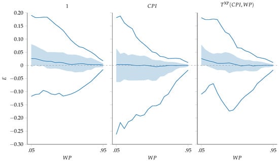
Figure 3. Functional boxplots of cost forecasting models implementing standard PFs and the best-performing progress-based PF.

Figure 4 displays the functional boxplots of the forecasting errors of the $tEAC$ models implementing 1, $SP{I}^{\mathrm{EVM}}$, $SP{I}^{\mathrm{ES}}$, and the best progress-based $sPF$ from Table 4, i.e., $T^{\mathrm{WAXP}}(CPI,E{S}_{\mathrm{s}},WP)$. Regarding the standard PFs, 1 performed best across all stages. Using $SP{I}^{\mathrm{EVM}}$ as the $sPF$ in Equation (8) instead of Equation (4) provided more accurate and precise results, yet fell behind other $sPF$s in performance. On the other hand, $T^{\mathrm{WAXP}}(CPI,E{S}_{\mathrm{s}},WP)$ performed the best, showing slightly narrower bounds and IQR throughout all the project phases.

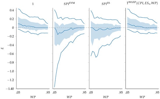
Figure 4. Functional boxplots of duration forecasting models implementing standard PFs and the best-performing progress-based PF.

5. Discussion

From a theoretical perspective, this study revealed multiple aspects. First, the progress-based PFs provided more accurate, precise, robust, and timely forecasts than the standard, combined, and average-based PFs for the dataset under analysis. The differences in the individual criteria were limited, especially when evaluated using scores calculated at the dataset level. However, when analyzed in aggregate and at the individual-project or physical-progress level, the differences in performance between progress-based and other PFs were more appreciable. Furthermore, even the slightest improvements could be crucial to project success in projects with hard budget or time constraints. This study also revealed that, in certain cases, the most effective cost-performance forecasting model ($cPF$) incorporated either $SP{I}^{\mathrm{EVM}}$ or $SP{I}^{\mathrm{ES}}$, while the most effective schedule-performance forecasting model ($sPF$) incorporated $CPI$. This could be due to two reasons. On the one hand, it is possible that cost performance was heavily influenced by schedule performance or vice versa. Alternatively, it may be that one of the indices exhibited greater stability, mitigating outliers in forecasting. This study also confirmed that the progress-based PFs consistently outperformed the other approaches. However, no progress-based PF or $PI$ (either physical or temporal) emerged as the clear winner. Therefore, it is recommended to consider forecasts from multiple PFs rather than relying solely on one.

From a practical perspective, this study provides guidance in developing progress-based PFs to change how estimates are evaluated during project execution without switching methods. Then, the study proposes a set of PFs developed following these principles, relying only on EVM and ES variables. While a particular PF may exhibit superior performance compared to others or even appear to be entirely disconnected from the project dynamics, its estimates should still be considered, complementing those derived from more suitable PFs or expert judgment.

The method adopted by the study has several limitations, all of which refer to Equation (20). First, the proposed progress-based PFs were developed using only $CPI$, $SP{I}^{\mathrm{EVM}}$, and $SP{I}^{\mathrm{ES}}$. Second, the evaluation of $xP{F}^{\prime }$ was limited to $\pm P{I}_x$. Third, the weights $[1-P_w\left(t\right)]$ and $P_w\left(t\right)$ that multiply 1 and $xP{F}^{\prime }$, respectively, could be reversed, just as 1 could be substituted. Lastly, no project critical phase was identified, as all progress stages (both in terms of physical progress and time progress) were accounted for in the same way. All these limitations were deliberately adopted to avoid further complicating the construction of the progress-based PFs. Future research may address all directions unexplored by the current study.

6. Conclusions

In project management, accurate and precise estimates are essential for making informed decisions regarding control actions and their scope. However, due to the inherent uncertainty in project activities, implementing the sophisticated estimation methods proposed in the literature is often impractical for practitioners. This study aimed to address this challenge by proposing a method that aligns with standard project-management practices while enhancing the reliability of estimates. Practitioners should readily adopt the proposed method and seamlessly integrate it with existing processes, ensuring its practical applicability and real-world impact.

The proposed method leverages the standard EVM and ES formulae to estimate project completion cost and duration. However, it introduces projection factors that account for physical project progress, temporal progress, or both. Progress is represented as an indicator that, through weighting or exponentiation, allows the PF to be adjusted from a conservative to a neutral value, effectively modifying the assumption underlying the remaining cost or duration calculation.

The study tested 71 PFs on 65 real projects for cost and duration-to-completion forecasting for 1235 total observations, each corresponding to a discrete advancement of physical progress. The results, analyzed across the board, at the individual-project level and the individual-percentage-of-physical-progress level, show that progress-based PFs can provide more accurate, precise, and timely forecasts. The most significant improvement was perceived in precision, followed by timeliness, and then by accuracy. In contrast to the sophisticated methods predicted in the literature, although the performance improvement over standard methodologies was limited, the proposed PFs were absolutely straightforward as they were based entirely on the same metrics predicted by the standard methodologies.

This study faced the limitation of using only EVM and ES metrics in the construction of the progress-based PFs. While these metrics provide valuable insights into project performance, they may not capture the full spectrum of factors that influence project progress and potential deviations from the original plan. Future research could explore the inclusion of additional variables, such as the project’s complexity, the experience of the project team, and external market conditions, to enhance the predictive power of the proposed method. Another limitation lies in the dependence on the project dataset used. Future studies could broaden the sample of projects analyzed.

References

- Rezakhani, P. Hybrid fuzzy-Bayesian decision support tool for dynamic project scheduling and control under uncertainty. Int. J. Constr. Manag. 2020, 22, 2864–2876. [Google Scholar] [CrossRef]
- Kwon, H.; Kang, C.W. Improving Project Budget Estimation Accuracy and Precision by Analyzing Reserves for Both Identified and Unidentified Risks. Proj. Manag. J. 2019, 50, 86–100. [Google Scholar] [CrossRef]
- Project Management Institute. Practice Standard for Project Risk Management, 1st ed.; Project Management Institute: Newton Square, PA, USA, 2009; p. 116. [Google Scholar]
- Abdel-Monem, M.; Alshaer, K.T.; El–Dash, K. Assessing Risk Factors Affecting the Accuracy of Conceptual Cost Estimation in the Middle East. Buildings 2022, 12, 950. [Google Scholar] [CrossRef]
- Project Management Institute. Practice Standard for Earned Value Management, 2nd ed.; Project Management Institute: Newton Square, PA, USA, 2012; p. 135. [Google Scholar]
- Lipke, W. Schedule is Different. Meas News 2003, 2, 31–34. [Google Scholar]
- Mayo-Alvarez, L.; Alvarez-Risco, A.; Del-Aguila-Arcentales, S.; Sekar, M.C.; Yañez, J.A. A Systematic Review of Earned Value Management Methods for Monitoring and Control of Project Schedule Performance: An AHP Approach. Sustainability 2022, 14, 5259. [Google Scholar] [CrossRef]
- Du, J.; Kim, B.C.; Zhao, D. Cost Performance as a Stochastic Process: EAC Projection by Markov Chain Simulation. J. Constr. Eng. Manag. 2016, 142, 4016009. [Google Scholar] [CrossRef]
- Barrientos, A.; Barrientos-Orellana, A.; Ballesteros-Pérez, P.; Mora-Melia, D.; González-Cruz, M.C.; Vanhoucke, M. Stability and accuracy of deterministic project duration forecasting methods in earned value management. Eng. Constr. Arch. Manag. 2021, 29, 1449–1469. [Google Scholar] [CrossRef]
- Aramali, V.; Gibson, G.E.; El Asmar, M.; Cho, N. Earned Value Management System State of Practice: Identifying Critical Subprocesses, Challenges, and Environment Factors of a High-Performing EVMS. J. Manag. Eng. 2021, 37, 04021031. [Google Scholar] [CrossRef]
- Li, M.; Zhou, H.; Zhang, R. A Dynamic Measurement Model of Equipment Procurement Progress for Nuclear Power Project Based on EVM. In Proceedings of the ASME 2017 Power Conference Joint with ICOPE-17 collocated with the ASME 2017 11th International Conference on Energy Sustainability, the ASME 2017 15th International Conference on Fuel Cell Science, Engineering and Technology, and the ASME 2017 Nuclear Forum, Charlotte, NC, USA, 26–30 June 2017; p. V002T07A003. [Google Scholar] [CrossRef]
- Fleming, Q.W.; Koppelman, J.M. Earned Value Project Management; Project Management Institute: Newton Square, PA, USA, 2016. [Google Scholar] [CrossRef]
- Batselier, J.; Vanhoucke, M. Empirical Evaluation of Earned Value Management Forecasting Accuracy for Time and Cost. J. Constr. Eng. Manag. 2015, 141, 5015010. [Google Scholar] [CrossRef]
- Kim, D.B.; White, E.D.; Ritschel, J.D.; Millette, C.A. Revisiting reliability of estimates at completion for department of defense contracts. J. Public Procure 2019, 19, 186–200. [Google Scholar] [CrossRef]
- Khamooshi, H.; Golafshani, H. EDM: Earned Duration Management, a new approach to schedule performance management and measurement. Int. J. Proj. Manag. 2014, 32, 1019–1041. [Google Scholar] [CrossRef]
- Chang, H.K.; Yu, W.D.; Cheng, T.M. A Quantity-Based Method to Predict More Accurate Project Completion Time. KSCE J. Civ. Eng. 2020, 24, 2861–2875. [Google Scholar] [CrossRef]
- Henderson, K. Further Developments in Earned Schedule. Meas News 2004, 2004, 15–22. [Google Scholar]
- Colin, J.; Martens, A.; Vanhoucke, M.; Wauters, M. A multivariate approach for top-down project control using earned value management. Decis. Support Syst. 2015, 79, 65–76. [Google Scholar] [CrossRef]
- Ballesteros-Pérez, P.; Sanz-Ablanedo, E.; Mora-Melià, D.; González-Cruz, M.; Fuentes-Bargues, J.L.; Pellicer, E. Earned Schedule min-max: Two new EVM metrics for monitoring and controlling projects. Autom. Constr. 2019, 103, 279–290. [Google Scholar] [CrossRef]
- Ngo, K.A.; Lucko, G.; Ballesteros-Pérez, P. Continuous earned value management with singularity functions for comprehensive project performance tracking and forecasting. Autom. Constr. 2022, 143, 104583. [Google Scholar] [CrossRef]
- Zwikael, O.; Globerson, S.; Raz, T. Evaluation of Models for Forecasting the Final Cost of a Project. Proj. Manag. J. 2000, 31, 53–57. [Google Scholar] [CrossRef]
- Anbari, F.T. Earned Value Project Management Method and Extensions. Proj. Manag. J. 2003, 34, 12–23. [Google Scholar] [CrossRef]
- Lipke, W. Independent estimates at completion—Another method. Meas. News 2004, 11, 10–14. [Google Scholar]
- Koke, B.; Moehler, R.C.R.C. Earned Green Value management for project management: A systematic review. J. Clean. Prod. 2019, 230, 180–197. [Google Scholar] [CrossRef]
- Barrientos-Orellana, A.; Ballesteros-Pérez, P.; Mora-Meliá, D.; Cerezo-Narváez, A. Comparison of the Accuracy of Cost Prediction Methods with Earned Value Analysis. In Proceedings of the 26 th International Congress on Project Management and Engineering, Terrassa, Spain, 5–8 July 2022; pp. 12–21. [Google Scholar]
- Henderson, K. Earned Schedule: A Breakthrough Extension to Earned Value Theory? A Retrospective Analysis of Real Project Data. Meas News 2003, 1, 13–23. [Google Scholar]
- Lipke, W.; Zwikael, O.; Henderson, K.; Anbari, F. Prediction of project outcome. Int. J. Proj. Manag. 2009, 27, 400–407. [Google Scholar] [CrossRef]
- Christensen, D.S. The estimate at completion problem: A review of three studies. Proj. Manag. J. 1993, 24, 37–42. [Google Scholar]
- Christensen, D.S.; Antolini, R.C.; McKinney, J.W. A Review of Estimate at Completion Research. J. Cost. Anal. 1995, 12, 41–62. [Google Scholar] [CrossRef]
- Batselier, J.; Vanhoucke, M. Improving project forecast accuracy by integrating earned value management with exponential smoothing and reference class forecasting. Int. J. Proj. Manag. 2017, 35, 28–43. [Google Scholar] [CrossRef]
- Martens, A.; Vanhoucke, M. Integrating Corrective Actions in Project Time Forecasting Using Exponential Smoothing. J. Manag. Eng. 2020, 36, 4020044. [Google Scholar] [CrossRef]
- Zhao, M.; Zi, X. Using Earned Value Management with exponential smoothing technique to forecast project cost. J. Phys. Conf. Ser. 2021, 1955, 12101. [Google Scholar] [CrossRef]
- Narbaev, T.; De Marco, A. Earned value and cost contingency management: A framework model for risk adjusted cost forecasting. J. Mod. Proj. Manag. 2017, 4, 12–19. [Google Scholar]
- De Marco, A.; Narbaev, T.; Ottaviani, F.M.; Vanhoucke, M. Influence of cost contingency management on project estimates at completion. Int. J. Constr. Manag. 2023, 1–11. [Google Scholar] [CrossRef]
- Warburton, R.D.H.; Cioffi, D.F. Estimating a project’s earned and final duration. Int. J. Proj. Manag. 2016, 34, 1493–1504. [Google Scholar] [CrossRef]
- Warburton, R.D.H.; Ottaviani, F.M.; De Marco, A. Critical Analysis of Linear and Nonlinear Project Duration Forecasting Methods. J. Mod. Proj. Manag. 2023, 11, 186–199. [Google Scholar]
- Zafari, B.; Kettunen, J. Bayesian Methods in Project Management. In Wiley StatsRef: Statistics Reference Online; Wiley: Hoboken, NJ, USA, 2017; pp. 1–5. [Google Scholar] [CrossRef]
- Firouzi, A.; Khayyati, M. Bayesian Updating of Copula-Based Probabilistic Project-Duration Model. J. Constr. Eng. Manag. 2020, 146, 4020046. [Google Scholar] [CrossRef]
- Caron, F. Project Control Using a Bayesian Approach. In Encyclopedia of Information Science and Technology, 4th ed.; IGI Global: Berlin/Heidelberg, Germany, 2018; pp. 5679–5689. [Google Scholar] [CrossRef]
- Mostafa, K.; Hegazy, T. Potential of Bayesian networks for forecasting the ripple effect of progress events. In Proceedings of the CSCE Annual Conference Growing with Youth, Laval, QC, Canada, 12–15 June 2019. [Google Scholar]
- Elmousalami, H.H. Artificial Intelligence and Parametric Construction Cost Estimate Modeling: State-of-the-Art Review. J. Constr. Eng. Manag. 2020, 146, 3119008. [Google Scholar] [CrossRef]
- Awada, M.; Srour, F.J.; Srour, I.M. Data-Driven Machine Learning Approach to Integrate Field Submittals in Project Scheduling. J. Manag. Eng. 2021, 37, 4020104. [Google Scholar] [CrossRef]
- Araba, A.M.; Memon, Z.A.; Alhawat, M.; Ali, M.; Milad, A. Estimation at Completion in Civil Engineering Projects: Review of Regression and Soft Computing Models. Knowl.-Based Eng. Sci. 2021, 2, 1–12. [Google Scholar] [CrossRef]
- Balali, A.; Valipour, A.; Antucheviciene, J.; Šaparauskas, J. Improving the results of the earned value management technique using artificial neural networks in construction projects. Symmetry 2020, 12, 1745. [Google Scholar] [CrossRef]
- Cheng, M.Y.; Hoang, N.D. Interval estimation of construction cost at completion using least squares support vector machine. J. Civ. Eng. Manag. 2014, 20, 223–236. [Google Scholar] [CrossRef]
- Wauters, M.; Vanhoucke, M. A comparative study of Artificial Intelligence methods for project duration forecasting. Expert Syst. Appl. 2016, 46, 249–261. [Google Scholar] [CrossRef]
- He, S.; Du, J.; Huang, J.Z. Singular-Value Decomposition Feature-Extraction Method for Cost-Performance Prediction. J. Comput. Civ. Eng. 2017, 31, 4017043. [Google Scholar] [CrossRef]
- Wauters, M.; Vanhoucke, M. A Nearest Neighbour extension to project duration forecasting with Artificial Intelligence. Eur. J. Oper. Res. 2017, 259, 1097–1111. [Google Scholar] [CrossRef]
- Santos, R.; Costa, A.A.; Grilo, A. Bibliometric analysis and review of Building Information Modelling literature published between 2005 and 2015. Autom. Constr. 2017, 80, 118–136. [Google Scholar] [CrossRef]
- Wauters, M.; Vanhoucke, M. Support Vector Machine Regression for project control forecasting. Autom. Constr. 2014, 47, 92–106. [Google Scholar] [CrossRef]
- Santos, J.I.; Pereda, M.; Ahedo, V.; Galán, J.M. Explainable machine learning for project management control. Comput. Ind. Eng. 2023, 180, 109261. [Google Scholar] [CrossRef]
- Liang, A.; Tao, L.; Lei, H. Combined machine-learning and EDM to monitor and predict a complex project with a GERT-type network: A multi-point perspective. Comput. Ind. Eng. 2023, 180, 109256. [Google Scholar] [CrossRef]
- Cheng, M.Y.; Chang, Y.H.; Korir, D. Novel Approach to Estimating Schedule to Completion in Construction Projects Using Sequence and Nonsequence Learning. J. Constr. Eng. Manag. 2019, 145, 4019072. [Google Scholar] [CrossRef]
- Al Hares, E.F.T.; Budayan, C. Estimation at completion simulation using the potential of soft computing models: Case study of construction engineering projects. Symmetry 2019, 11, 190. [Google Scholar] [CrossRef]
- Kareem Kamoona, K.R.; Budayan, C. Implementation of Genetic Algorithm Integrated with the Deep Neural Network for Estimating at Completion Simulation. Adv. Civ. Eng. 2019, 2019, 7081073. [Google Scholar] [CrossRef]
- Le, T.A.; Huynh, Q.T.; Nguyen, T.H.; Nguyen, N.H.; Cao, P.N. A Method for Project Completion Cost Predicting Using LSTM in Earned Value Management Technique. In Proceedings of the 2020 4th International Conference on Recent Advances in Signal Processing, Telecommunications & Computing (SigTelCom), Hanoi, Vietnam, 28–29 August 2020; pp. 87–92. [Google Scholar] [CrossRef]
- Aidan, I.A.; Al-Jeznawi, D.; Al-Zwainy, F.M.S.S. Predicting earned value indexes in residential complexes’ construction projects using artificial neural network model. Int. J. Intell. Eng. Syst. 2020, 13, 248–259. [Google Scholar] [CrossRef]
- Mohammed, S.J.; Abdel-khalek, H.A.; Hafez, S.M. Predicting Performance Measurement of Residential Buildings Using Machine Intelligence Techniques (MLR, ANN and SVM). Iran. J. Sci. Technol.-Trans. Civ. Eng. 2021, 46, 3429–3451. [Google Scholar] [CrossRef]
- Dastgheib, S.R.; Feylizadeh, M.R.; Bagherpour, M.; Mahmoudi, A. Improving estimate at completion (EAC) cost of construction projects using adaptive neuro-fuzzy inference system (ANFIS). Can. J. Civ. Eng. 2022, 49, 222–232. [Google Scholar] [CrossRef]
- Vanhoucke, M. The Illusion of Control: Project Data, Computer Algorithms and Human Intuition for Project Management and Control, 1st ed.; Springer: Berlin/Heidelberg, Germany, 2023; p. 330. [Google Scholar] [CrossRef]
Disclaimer/Publisher’s Note: The statements, opinions and data contained in all publications are solely those of the individual author(s) and contributor(s) and not of MDPI and/or the editor(s). MDPI and/or the editor(s) disclaim responsibility for any injury to people or property resulting from any ideas, methods, instructions or products referred to in the content. |
© 2024 by the authors. Licensee MDPI, Basel, Switzerland. This article is an open access article distributed under the terms and conditions of the Creative Commons Attribution (CC BY) license (https://creativecommons.org/licenses/by/4.0/).