Development and Verification of Wireless Vibration Sensors

Abstract

Structural vibration testing is an effective guarantee for the Structural Health Monitoring (SHM) of large-scale civil engineering. Traditional vibration testing has drawbacks such as difficulties in wiring and picking up low-frequency signals, low communication speed, and susceptibility to testing site conditions. In order to improve the universality of wireless vibration sensors, this article develops a wireless vibration sensor, introduces the module composition and basic principles of the sensor, and conducts standard vibration table performance comparison tests between wired acceleration sensors and wireless vibration sensors, verifying the accuracy of wireless vibration sensors. In order to further explore the feasibility of wireless vibration sensor applications, the wired acceleration sensor and wireless vibration sensor were used to analyze the structural dynamic characteristics of the four-layer steel frame structure model in the laboratory, and the comparison was made based on ABAQUS finite element simulation. Finally, the field vibration test was carried out outdoors. The results show that the natural frequency identification results of the wireless vibration sensor and the wired acceleration sensor for the four-story steel frame structure through fast Fourier transform, short-time Fourier transform, and wavelet transform are basically the same, the half-power bandwidth method and logarithmic decrement rate method are used to identify the damping, and wavelet transform is used to identify the vibration mode with minimal error and high accuracy. It shows that the wireless vibration sensor is feasible in practical engineering, has stable and reliable transmission capacity, and can provide certain reference values for earthquake monitoring, building Structural Health Monitoring, etc.

1. Introduction

The design service life of building structures is generally 50 years, but, with the accumulation of time and the influence of external environment, many buildings begin to experience a series of health problems, such as cumulative aging and damage to structures, slight changes in structural deformation, and internal damage to structures. Many health issues can affect the applicability, safety, and durability of structures [1,2,3]. Ensuring structural safety is the top concern of engineers. In recent years, engineering accidents have occurred frequently due to neglecting or neglecting structural health issues, such as the collapse of the FIU pedestrian bridge in Miami, USA, and the collapse of the New Home Hotel in Quanzhou, China. The above engineering cases illustrate that the health issues of exposed structures such as bridges, dams, and high-rise buildings in nature need to be put on the agenda as soon as possible. For buildings with structures that have reached their designed lifespan, although they can be used normally for a certain period of time, there are still certain risks [4,5]. To avoid accidents or minimize losses caused by accidents, regular or even long-term health monitoring of building structures is necessary. Therefore, it is very necessary to conduct health monitoring and safety assessment on civil engineering structures [6,7,8].

Structural health detection technology refers to the use of on-site non-destructive and real-time methods to collect input and output information of structures, analyze structural fluctuations, deterioration, damage, and other characteristics, and provide decision-making support for management and maintenance. At present, the main methods of structural health detection in various countries include wired testing and wireless testing [9,10]. The traditional Structural Health Monitoring system usually uses wired sensors to measure the building’s structure. Although this method will make the measured data synchronized quickly, there will be many inconveniences in the layout of measuring points. On the one hand, due to the fact that measurement points are usually arranged on different floors, it not only increases the workload of early wiring but also cannot guarantee the stability between equipment. On the other hand, after completing the tedious wiring work in the early stage, it is also necessary to consider the attenuation problem of the collected signal during long-distance transmission, and the attenuation rate of signal transmission will change with the distance between measurement points, thereby affecting data analysis [11,12,13,14]. With the rapid development of wireless network technology, wireless sensor network technology represented by the Internet of Things is widely used in the research field of Structural Health Monitoring [15,16]. Zhang et al. comprehensively reviewed the radio frequency identification sensor system used for Structural Health Monitoring in recent years. As the radio frequency technology is suitable for short distance transmission, its use is limited [17]. In order to overcome the shortcomings of short distance transmission in frequency transmission technology, a new generation of Zigbee technology is gradually emerging. Yan et al. proposed a wireless sensor network monitoring technology based on Zigbee 802.15.4 protocol and carried out dynamic stress monitoring and internal crack detection on large building structures. However, Zigbee technology is suitable for data transmission between various electronic devices with close ranges, low power consumptions, and low transmission rates [18,19]. Although WiFi has the disadvantage of high power consumption, it has certain advantages over Zigbee and frequency technology in terms of transmission speed and distance. Heo et al. developed a Wireless Unified Maintenance System (WUMS) to meet all the requirements of a civil structural disaster prevention SHM system. This system allows users to selectively use the WiFi RF frequency band to measure structural response in real time, provided that WiFi has a wider bandwidth and stronger frequency signal [20]. To create a low-cost and easy to implement Structural Health Monitoring method, many scholars have proposed to use the built-in sensors, network transmission, data storage, and embedded processing functions in modern smart phones to achieve Structural Health Monitoring. A large number of experiments have proved that smart phones can not only become useful wireless sensor network (WSN) components, forming a self-management SHM system, they can also be used for long-term determination of structural damage [21,22,23]. However, with the rapid development of building informatization, some scholars have begun to attempt to develop and combine health monitoring systems based on existing BIM technology and have come to the conclusion that not only can a considerable amount of sensor data be obtained by fully utilizing the advantages of BIM, but, also, subsequent structural health information can be obtained [24,25]. As we all know, the offshore building structures suffering from severe marine environment need higher level Structural Health Monitoring technology. Chandrasekaran et al. could easily identify structural damage by deploying dense array sensors to monitor reaction behavior [26]. To further overcome the adaptability and complexity of offshore sites, Kim et al. proposed a method of comparing cosine similarity with sensor data, which could directly identify the most similar situation to the current state without any additional analysis between monitoring and damage identification, making the damage identification process simpler [27]. Due to poor monitoring conditions, Zhao et al. proposed a Structural Health Monitoring method based on the baseline model to eliminate the impact of external environment on Structural Health Monitoring, mainly by establishing the relationship between signal characteristics and changing environment, then using data statistical analysis to assess the tolerance range of signal characteristics [28]. However, other protocols are also used in the development of wireless sensors, especially Bluetooth Low Energy and LoRa, which are widely used in on-site Structural Health Monitoring with low costs and low power consumptions [29,30]. The above research fully showed that wireless sensor network technology could not only solve the problems of wired sensor layout difficulties and high maintenance costs but also collect monitoring data with high accuracies and a large number of advantages, such as real-time monitoring, pre-processing of collected data, etc. Therefore, wireless sensor technology has developed rapidly [31,32,33,34,35,36,37,38].

To sum up, in order to improve the data transmission accuracy of the wireless vibration sensor and the flexibility of the field application, this paper developed a high-precision wireless vibration sensor that could choose different wireless communication modes (4G and WiFi) according to the field environment. The standard vibration table performance comparison test was carried out in the laboratory, and the test results showed that the wireless vibration sensor was accurate and reliable. Then, the numerical simulation and indoor vibration test of the four-layer steel frame scale model were carried out in the laboratory, and it was found that the dynamic characteristics of the structure obtained by the two methods were basically consistent. Finally, the wireless vibration sensor and the wired acceleration sensor were tested in the field, and the test results showed that the data accuracy could meet the actual engineering monitoring requirements. The above tests demonstrated that the developed wireless vibration sensors could be used in the field of Structural Health Monitoring in civil engineering.

2. Hardware Design of Wireless Vibration Sensors

The overall structure of wireless vibration sensors is mainly composed of a data acquisition module, a signal processing module, a data transmission module, a power supply module, etc. The overall structure is shown in Figure 1. In the data acquisition module, the sensor detects and sends the measured signal to a high-precision analog-to-digital conversion unit after a series of processing, which is then converted into a digital signal and stored in a storage unit (Micro SD card). At the same time, the signal can also be sent to the upper computer through a 4G communication module or WiFi communication module through processor allocation. Among them, the signal processing module mainly includes an anti aliasing filter, a programmable amplifier PGA281, and a 24-bit, high-precision analog-to-digital converter. Processors are usually connected to storage units, are mainly used to manage the current system’s processing processes, and work together with other modules to complete assigned monitoring tasks. In addition to various functional modules, another important component is the power supply module (battery powered, based on time history sampled at 50 Hz for 60 s, the battery supply time is estimated to be approximately 24 h), which will provide power to each module of the wireless vibration sensor and maintain normal operation. The internal structure and external overall physical image of the wireless vibration sensor are shown in Figure 2.

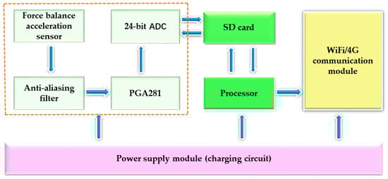
Figure 1. Overall structure of wireless vibration sensors.

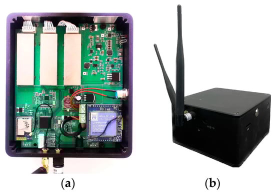
Figure 2. Physical diagram of wireless vibration sensor. (a) Internal structure diagram; (b) External physical image.

2.1. Data Acquisition Module

The specific process of the data collection module is shown in Figure 3. The force-balanced acceleration sensor filters the measured signal through an anti-aliasing filter to obtain an accurate electrical signal based on the sampling frequency. The signal is then amplified by a programmable amplifier (PGA281) to maintain its original state. Finally, the conditioned signal is transmitted to a 24-bit analog-to-digital converter (ADC).

Figure 3. Basic structure of signal conditioning.

2.2. Signal Processing Module

This article adopts a force-balanced acceleration sensor, which can measure low-frequency and ultra-low frequency vibrations of a structure. The main principle is to convert the external measured single component vibration acceleration signal into a voltage digital signal inside the sensor. It has the advantages of high sensitivity, high measurement accuracy, good consistency of technical parameters, small size, low power consumption, and good stability. Compared with MEMS acceleration sensors, MEMS acceleration sensors generally have a measurement dynamic range of −70 dB, whereas force-balanced acceleration sensors have a measurement dynamic range greater than 120 dB. Thus, MEMS acceleration sensors are mainly used in larger vibration signal measurement fields, such as automobiles, various mechanical fields, etc. [39], and force-balanced acceleration sensors are mainly used in building structures, earthquake monitoring, etc. After the sensor completes the measurement work, due to the theoretically infinite frequency components contained in the measured signal, high-order modal frequencies are likely to overlap to the low frequency range, resulting in signal aliasing. Therefore, after the sensor collects the signal, it is necessary to perform low-pass filtering on the collected signal. Considering that the signal may experience attenuation during transmission, after low-pass filtering, a programmable amplifier is added to amplify the signal as necessary.

The sensor uses a programmable amplifier (PGA281) to amplify the electrical signal, and the circuit diagram is shown in Figure 4 (Figure 4 is sourced from https://www.ti.com/product/PGA281#tech-docs, accessed on 21 April 2023). The programmable amplifier (PGA281) is a high-precision instrument amplifier with CNC gain and signal integrity testing functions. It can provide multiple internal gain options within the range of 1/8 V/V (attenuation) to 176 V/V, making it highly versatile and suitable for various analog front-end applications. At the same time, the signal rail to rail output is a wide range input, which makes the docking work between the programmable amplifier PGA281 and the low voltage domain of the high-resolution analog-to-digital converter (ADC) easy.

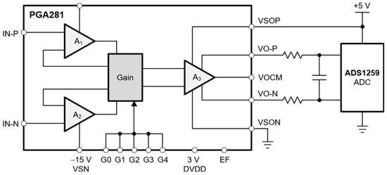
Figure 4. PGA281 circuit diagram.

2.3. Data Processing Module

Large building structures usually undergo long-term monitoring work; thus, it is necessary to consider factors such as data transmission accuracy, data processing and analysis capabilities, and power consumption impact. The sensor uses a high-precision and low-power STM32F429 micro-controller as the main CPU controller [40]. STM32F429 is a micro-controller based on the high-performance ARM Cortex-M4 32-bit RISC core. It has a working frequency of up to 180 MHz, a working temperature range of −40~+105 °C, and a power supply voltage range of 1.7~3.6 V. The core of the micro-controller comes with a single precision floating-point unit (FPU) that supports all AMR single precision data processing instructions and data types. It is suitable for efficient allocation and high-precision data processing under ultra long-distance testing conditions.

2.4. Power Supply Management Module

The power management module of wireless vibration sensors needs to consider the overall charging stability, as well as the stability and interference of reference voltages such as the STM32F429 microprocessor, the 4G and WiFi communication module, the programmable amplifier, the analog-to-digital converter, etc. Thus, we use a low-cost and highly stable constant current and voltage charger, SJT-30W, which can adjust the charging current through peripheral resistors to ensure overall charging stability. The power module includes a +12 V battery and the DC/DC modules DS1 and DS2. Considering the rated working voltage of the STM32F429 micro-controller, 4G and WiFi communication module, and signal conditioning circuit in the system, in the design of power management, the DC/DC module DS1 converts the +12 V power supply into a +/−12 V dual power supply output, and the output +/−12 V power supply directly supplies power to the programmable amplifier PGA281. The DC/DC module DS2 converts the input power into a +5 V single power output, and the output power is supplied to the AD analog-to-digital converter and various chips through decoupling filtering capacitors C24 and C25. The size of the internal output voltage of the DC/DC module can be changed by controlling the duty cycle of the oscillation part to maintain a constant output. Compared with the voltage stabilization module, the entire voltage reduction process can minimize the consumption of electrical energy on the voltage reduction module, thereby ensuring the stability of circuit conditioning in wireless vibration sensors and the rationality of internal power supply. Figure 5 shows the schematic diagram of the power module circuit.

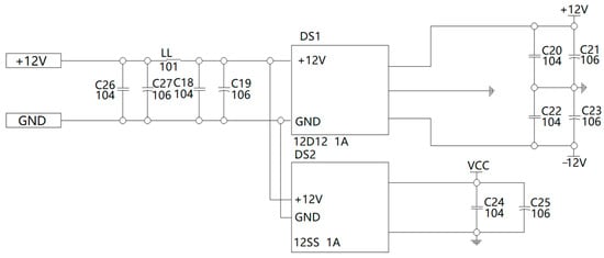
Figure 5. Schematic diagram of power module circuit.

2.5. Wireless Communication Module

Wireless vibration sensors mainly include two communication methods: 4G wireless communication and WiFi wireless communication. The corresponding communication method can be selected based on on-site measurement conditions. There is a slight difference in the communication chips used in the two communication methods. The WH-LTE-7S4 V2 communication chip is used for 4G wireless communication of the wireless vibration sensor (as shown in Figure 6), whereas the E103-W02 communication chip is used for WiFi wireless communication (as shown in Figure 7). The two chips have certain advantages in connection modes, data processing and analyses, hardware updates, power consumptions, stabilities, and reliabilities, and the WH-LTE-7S4V2 communication chip can establish powerful network nodes at low cost, thus adapting to the fields of Structural Health Monitoring and earthquake monitoring used for long-term work, ultra-long-distance testing, and large amounts of data processing.

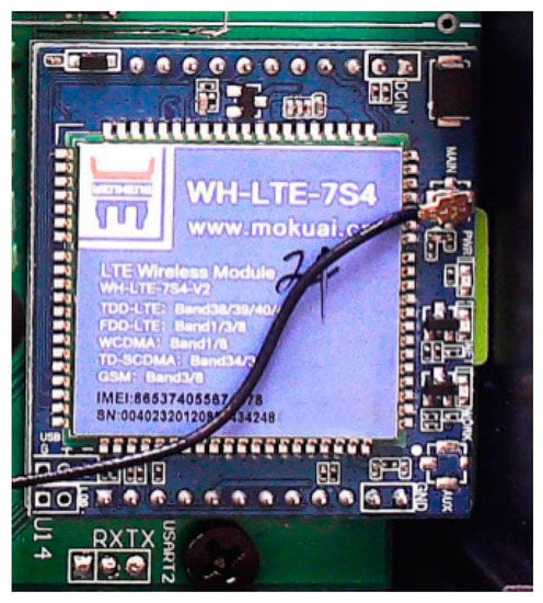
Figure 6. WH-LTE-7S4 V2 communication chip.

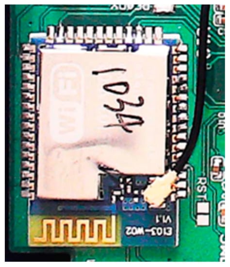
Figure 7. E103-W02 communication chip.

3. Visual Interface for Wireless Vibration Sensors

The data visualization interface of the wireless vibration sensor has the functions of monitoring equipment overview, data viewing, historical data playback, and relevant parameter data export. When it comes to short distance engineering vibration testing work, wireless vibration measurement systems can use WiFi for data transmission within the local area network. The system fixes the IP address of the server. After connecting the server computer to the router connected to the system, the IP address of the server computer itself needs to be fixed to 192.168.1.102 so that the server and system equipment can communicate in the same router environment. The connection interface is shown in Figure 8.

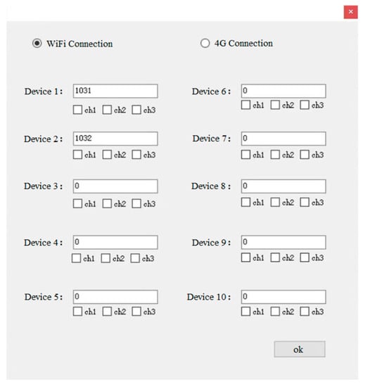
Figure 8. WiFi Connection Mode Interface.

Before data collection, it is necessary to set the sampling rate. After stopping collection, the collected data will be stored in the log directory under the running directory of the collection software. In actual large-scale construction engineering measurement work, it involves ultra-long-distance engineering testing tasks; thus, engineering vibration testing can be carried out based on the advantages of the 4G communication method, such as large coverage range, strong anti-interference ability, and high transmission rate. The 4G communication method requires inserting a 4G traffic card into the wireless vibration sensor and then turning on the power. After turning on the power, it takes about 1 min to connect to the operator’s network and then connect to the network cloud server. Before running the user application software, it is necessary to first install and run the cloud service serial port virtual software: USR-VCOM_V3.7.2.529_. Then, the user sets up and enters the username and password of the cloud server in the login interface of the software and then establishes a connection between the device and the virtual serial port (as shown in Figure 9). After the connection is completed, the data collection software is opened, and the user can proceed with the data collection work. The connection method of the data collection interface is the same as the WiFi connection method mentioned above. Two communication methods can be selected and used according to the on-site situation.

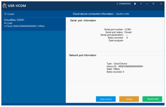
Figure 9. 4G communication mode login interface and serial port connection interface.

4. Performance Testing of Wireless Vibration Sensors

To verify the accuracy of wireless vibration sensors, the sensors are fixed in the middle of a single axis horizontal standard vibration table in the laboratory, and sine waves of different frequencies are input to test the amplitude frequency characteristics and amplitude linearity characteristics of the sensors. The vibration table is shown in Figure 10, and the specific performance parameters are shown in Table 1.

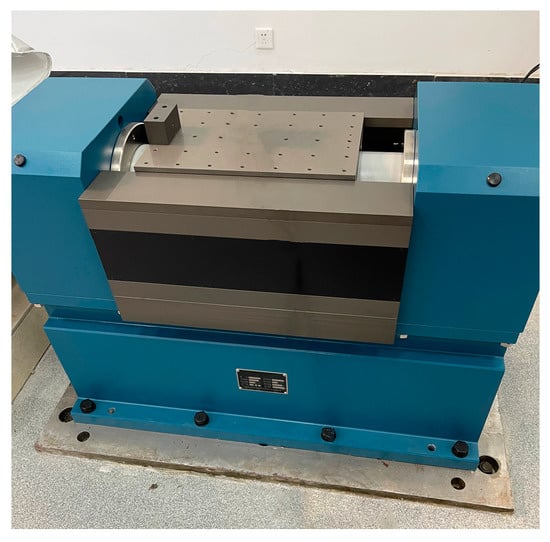
Figure 10. Vibration table.

Table 1. The main standard instruments of measurement.

Name	Measuring Range	Uncertainty	Accuracy	Maximum Permissible Error
Standard vibration table	(0.1–200) Hz	Urel = 0.5% (k = 2)	Urel = 1% (k = 2)	±0.1%

4.1. Sensitivity Amplitude Frequency Characteristic Test

In total, 14 frequency test points within the frequency range of 0.1 to 120 Hz were selected for sensitivity testing of the sensor. Due to the limitations of the maximum amplitude and maximum output acceleration of the low-frequency calibration vibration table, different accelerations (0.1, 0.2, 0.5, 1, 2, 5, 10 m/s²) were selected for testing at different frequency points. The measured results were compared with the static sensitivity, which was 278.9 mV/(m/s²) at 0 Hz. The test results are shown in Table 2.

Table 2. Sensitivity amplitude-frequency characteristic test results.

Frequency (Hz)	Output Acceleration (m/s2)	Sensitivity (mV/m/s2)	Urel,k = 2(%)
0.1	0.01	296.8	2.0
0.2	0.02	282.9	2.0
0.5	0.05	279.3	2.0
1	1.0	278.3	2.0
2	2.0	278.8	2.0
5	5.0	278.9	2.0
10	10.0	278.1	2.0
20	10.0	275.6	2.0
30	10.0	271.3	2.0
50	10.0	259.6	2.0
60	10.0	252.8	2.0
80	10.0	238.6	2.0
100	10.0	225.0	2.0
120	10.0	212.1	2.0

From the test results in Table 1, it can be seen that the sensitivity of the wireless vibration sensor in low-frequency testing is similar to the static sensitivity, with a maximum error of 0.51% in amplitude frequency characteristics, and the uncertainty of each group of data was two percent, indicating the high reliability of the test results.

4.2. Acceleration Amplitude Linear Test

The vibration table test signal frequency is selected as 10 Hz, and the acceleration amplitudes are selected as 0.1, 1, 5, 10, 20, and 30 m/s², respectively. The measured results are compared with the static sensitivity, and the static sensitivity (0 Hz) is 278.9 mV/(m/s²). The test results are shown in Table 3.

Table 3. Linear test results of acceleration amplitude.

Frequency (Hz)	Output Acceleration (m/s2)	Sensitivity (mV/m/s2)	Urel,k = 2(%)
10	0.1	278.8	2.0
10	1	278.5	2.0
10	5	278.5	2.0
10	10	278.4	2.0
10	20	278.1	2.0
10	30	278.1	2.0

From Table 3, it can be seen that when the sensor had a fixed test signal frequency of 10 Hz, and six different values of acceleration amplitude were selected. The maximum linearity error was 0.29%, and the corresponding output acceleration of the vibration table was 30 m/s². The uncertainty of each group of test data was two percent, indicating the high reliability of the test results.

5. Research on Dynamic Characteristics Based on Wireless Vibration Sensors

The pulsation and free decay tests were carried out using a scaled-down model located in the laboratory of the School of Construction Engineering at Dalian University. The model was a steel frame structure consisting mainly of four steel plates and four steel columns fastened together by high strength bolts, with the bottom of the model fixed to the laboratory floor by means of a fastening, thus ensuring the overall rigidity of the steel frame model. The total height of the building was 1000 mm, with a first-floor height of 350 mm, a second and third floor height of 200 mm, a fourth-floor height of 250 mm, and a steel plate size of 600 × 800 × 9 mm, steel column size 30 × 6 × 1000 mm. The specific dimensions of the model are shown in Figure 11, and the material properties of the steel columns and steel plates are shown in Table 4.

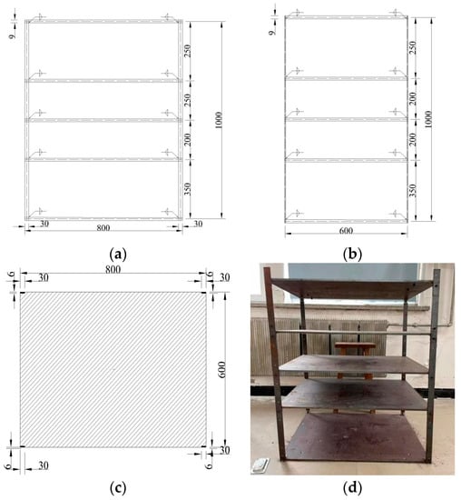
Figure 11. Scaled-down models of steel frame structures. (a) Front view; (b) side view; (c) steel plate; (d) steel-frame structure.

Table 4. Scale steel frame model member material.

Components	Material	Dimension (mm)	Density (g/cm3)	Young’s Modulus (GPa)	Poisson’s Ratio
Steel column	Q235	30 × 6	7.85	200	0.30
Steel plate	Q235	600 × 800	7.85	200	0.30

5.1. Modal Analysis of Scaled Steel Frames

Using the finite element software ABAQUS, establish a finite element model, as shown in Figure 12, based on the dimensions, materials, and connection methods of the scaled model of the laboratory steel frame structure and perform modal analysis. Among them, the steel plate selects the shell element (S4R), and the steel column selects the beam element (B31). Table 5 shows the first ten vibration modes of the scaled steel frame structure, and Figure 13 shows the first four vibration modes of the scaled steel frame structure model.

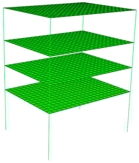
Figure 12. Finite element model.

Table 5. Modal characteristics of scaled steel frame structure model.

Vibration Mode	Frequency (Hz)	Time (s)	Characteristics
1	1.5326	0.6525	X
2	5.9878	0.1670	Y
3	6.0632	0.1650	torsion
4	6.7046	0.1492	torsion
5	15.350	0.0651	Y
6	19.121	0.0522	X
7	28.486	0.0351	torsion
8	31.564	0.0317	Y
9	32.593	0.0307	Z
10	32.823	0.0305	Z

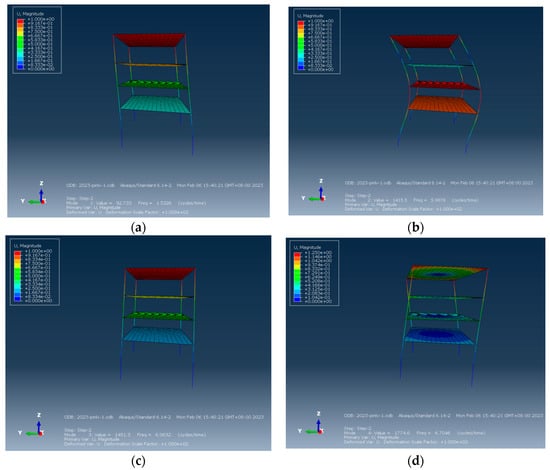
Figure 13. Vibration mode diagram of steel frame structure. (a) First-order vibration mode; (b) Second-order vibration mode; (c) Third-order vibration mode; (d) Fourth-order vibration mode.

5.2. Identification of Natural Frequency

5.2.1. Fast Fourier Transform (FFT)

FFT is a discrete Fourier transform algorithm commonly used in engineering vibration testing with a large number of sampling points. The specific process is to use a sliding window to obtain n consecutive time-domain data from the original signal, and then use the FFT method to convert the frequency information of each window data. The specific definition formula is as follows:

$$f(t)=\frac{1}{2\pi }{\displaystyle {\int }_{-\infty }^{+\infty }}F(jw)e^{jwt}d(w)$$

(1)

It is also possible to convert frequency domain signals into time domain:

$$F(jw)={\displaystyle {\int }_{-\infty }^{+\infty }}f(t)e^{jwt}d(t)$$

(2)

According to Formula (2), signals can be converted to each other in the frequency domain and time domain. In practical engineering, more accurate analysis signals can be obtained by using discretization Fourier transform, as shown in formula:

$$f(t)={\displaystyle \sum _{-\infty }^{+\infty }{c}_w}{e}^{jwt}$$

(3)

From this, it can be concluded that the main idea of FFT is to solve for the complex signal f(t) and then decompose it to obtain the sum of different sinusoidal signals. Additionally, the more sine signals obtained from f(t) decomposition the more frequency components they have.

(1)

Free attenuation test

The measurement points are selected as the center positions of each top layer of the steel frame structure, with measurement points 1 to 4 from bottom to top. After selecting the measurement points, wireless vibration sensors and wired acceleration sensors are arranged, and data collection work begins (as shown in Figure 14). After the experiment, perform fast Fourier transform on the measured data. During the testing process, the wireless vibration sensor and wired acceleration sensor have a sampling rate of 50 Hz and a sampling time of 1 min. The frequency of each order obtained from the data under the free attenuation test through fast Fourier transform and the natural vibration frequency of each order obtained from ABAQUS calculation results are shown in Table 6. The analysis results in the time and frequency domains of each measurement point are shown in Figure 15, Figure 16, Figure 17, Figure 18, Figure 19, Figure 20, Figure 21 and Figure 22. From the analysis of the results, it can be seen that the natural frequency distribution of wired, wireless, and ABAQUS is basically consistent during the sampling time.

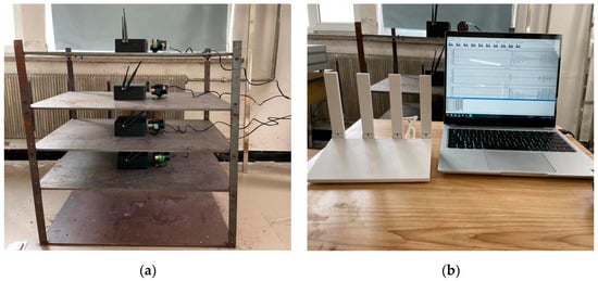
Figure 14. Layout of measurement points and data collection. (a) Measuring point layout; (b) data acquisition.

Table 6. Free attenuation test—comparison of natural frequency with FFT and ABAQUS calculation results.

Measure Point	Vibration Mode	Wireless Test Results (Hz)	Wired Test Results (Hz)	ABAQUS Analysis Results (Hz)
1	1	1.533840	1.533840	1.532600
	2	6.118710	6.118710	5.987800
	3	14.93831	14.93831	15.35000
2	1	1.533840	1.533840	1.532600
	2	6.118710	6.118710	5.987800
	3	14.93831	14.93831	15.35000
3	1	1.533840	1.533840	1.532600
	2	6.118710	6.118710	5.987800
	3	14.93831	14.93831	15.35000
4	1	1.533840	1.533840	1.532600
	2	6.118710	6.118710	5.987800
	3	14.93831	14.93831	15.35000

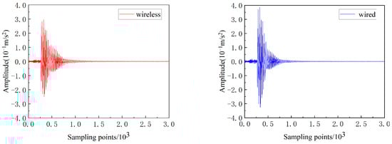
Figure 15. Time history curves of wireless and wired acceleration for No.1 measuring point under free attenuation test.

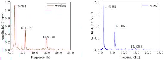
Figure 16. Frequency domains diagram of wireless and wired for No.1 measuring point under free attenuation test.

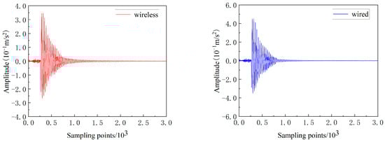
Figure 17. Time history curves of wireless and wired acceleration for No.2 measuring point under free attenuation test.

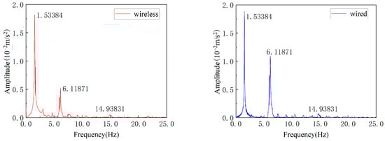
Figure 18. Frequency domains diagram of wireless and wired for No.2 measuring point under free attenuation test.

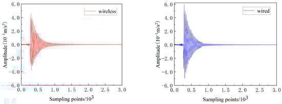
Figure 19. Time history curves of wireless and wired acceleration for No.3 measuring point under free attenuation test.

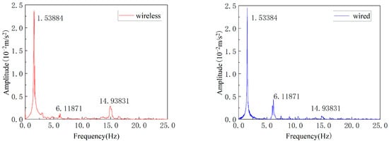
Figure 20. Frequency domains diagram of wireless and wired for No.3 measuring point under free attenuation test.

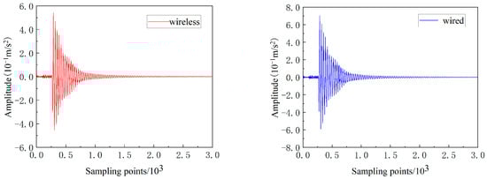
Figure 21. Time history curves of wireless and wired acceleration for No.4 measuring point under free attenuation test.

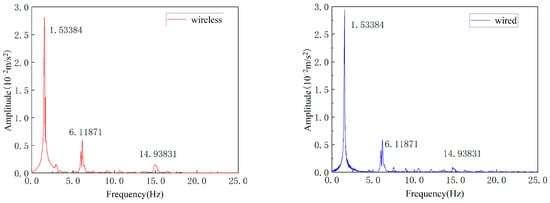
Figure 22. Frequency domains diagram of wireless and wired for No.4 measuring point under free attenuation test.

(2)

Pulsation test

The arrangement of measurement points for the pulsation test is the same as those for the free attenuation test (as shown in Figure 14). During the testing process, the wireless vibration sensor and wired acceleration sensor have a sampling rate of 50 Hz and a sampling time of 1 min. The various frequencies obtained from the pulsation test data through fast Fourier transform and the natural frequencies obtained from ABAQUS calculation results are shown in Table 7. The analysis results in the time and frequency domains of each measurement point are shown in Figure 23, Figure 24, Figure 25, Figure 26, Figure 27, Figure 28, Figure 29 and Figure 30. From the analysis of the results, it can be seen that the natural frequency distribution of wired, wireless, and ABAQUS is basically consistent during the sampling time.

Table 7. Pulsation test—comparison of natural frequency with FFT and ABAQUS calculation results.

Measure Point	Vibration Mode	Wireless Test Results (Hz)	Wired Test Results (Hz)	ABAQUS Analysis Results (Hz)
1	1	1.683330	1.683330	1.532600
	2	6.450000	6.450000	5.987800
	3	15.08333	15.08333	15.35000
	4	21.16677	21.16677	19.12100
2	1	1.683330	1.683330	1.532600
	2	6.450000	6.450000	5.987800
	3	15.08333	15.08333	15.35000
	4	21.16677	21.16677	19.12100
3	1	1.683330	1.683330	1.532600
	2	6.450000	6.450000	5.987800
	3	15.08333	15.08333	15.35000
	4	21.16677	21.16677	19.12100
4	1	1.683330	1.683330	1.532600
	2	6.450000	6.450000	5.987800
	3	15.08333	15.08333	15.35000
	4	21.16677	21.16677	19.12100

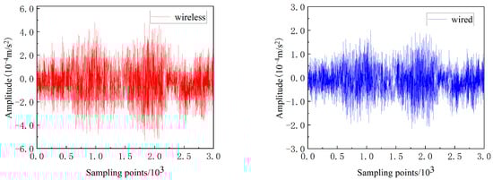
Figure 23. Time history curves of wireless and wired for No.1 measuring point under pulsation test.

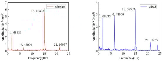
Figure 24. Frequency domains diagram of wireless and wired for No.1 measuring point under pulsation test.

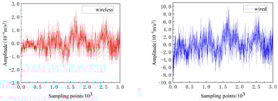
Figure 25. Time history curves of wireless and wired for No.2 measuring point under pulsation test.

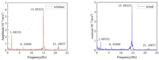
Figure 26. Frequency domains diagram of wireless and wired for No.2 measuring point under pulsation test.

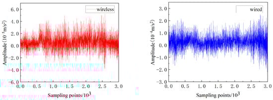
Figure 27. Time history curves of wireless and wired for No.3 measuring point under pulsation test.

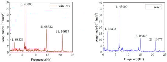
Figure 28. Frequency domains diagram of wireless and wired for No.3 measuring point under pulsation test.

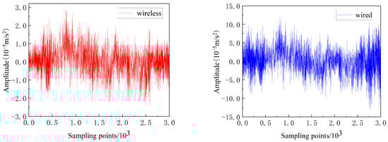
Figure 29. Time history curves of wireless and wired for No.4 measuring point under pulsation test.

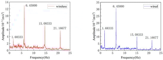
Figure 30. Frequency domains diagram of wireless and wired for No.4 measuring point under pulsation test.

The results obtained from the FFT of the field measurements of wired acceleration sensors and wireless vibration sensors were compared with the results calculated by ABAQUS for analytical error analysis, and the results are shown in Table 8 and Table 9:

Table 8. Error analysis of free attenuation test.

Vibration Mode	Frequency (Hz)			Relative Error (%)		Characteristics
	Wireless	Wired	ABAQUS	Test	ABAQUS
1	1.533840	1.533840	1.532600	0	0.08	X
2	6.118710	6.118710	5.987800	0	2.18	Y
3			6.063200			torsion
4			6.704600			torsion
5	15.08333	15.08333	15.35000	0	1.76	Y
6			19.12100			X
7			28.48600			torsion
8			31.56400			Y
9			32.59300			Z
10			32.82300			Z

Table 9. Error analysis of the pulsation test.

Vibration Mode	Frequency (Hz)			Relative Error (%)		Characteristics
	Wireless	Wired	ABAQUS	Test	ABAQUS
1	1.683330	1.683330	1.593600	0	5.63	X
2	6.450000	6.450000	5.987800	0	7.70	Y
3			6.063200			torsion
4			6.704600			torsion
5	15.08333	15.08333	15.35000	0	1.76	Y
6	21.16677	21.16677	19.12100	0	10.7	X
7			28.48600			torsion
8			31.56400			Y
9			32.59300			Z
10			32.82300			Z

The above results indicate that the wireless and wired test results of the free attenuation test and the pulsation test are consistent. For the free attenuation test, the difference between the wireless and wired test results and the ABAQUS calculation results is very small, with the maximum difference being the second order mode shape, reaching 2.18%. For the pulsation test, the difference between the wireless and wired test results and the ABAQUS calculation results is also very small, with the maximum difference being the fourth-order vibration mode, reaching 10.7%. The reason for its deviation may be due to differences between the parameters used in ABAQUS modeling and the actual structure.

5.2.2. Short Time Fourier Transform (STFT)

STFT is obtained from time-frequency analysis of Fourier transform localization. The principle of STFT is to first divide the time-domain signal into several narrow time periods along the time axis, and then perform Fourier transform on the signal within each time period. Then, the physical characteristics of the signal in each small time period can be obtained, and the narrow time periods that are divided into are called the windows of Fourier Transform. The specific expression for the STFT is as follows:

$$\mathrm{STFT}\left(t,f\right)={\displaystyle {\int }_{-\infty }^{+\infty }s\left(\tau \right)}g\left(\tau -t\right)e^{-j^2\pi f\tau }dt$$

(4)

In the above expression:

• $f\left(t\right)\in L^2\left(R\right),$
• g(t)—window function;
• s(t)—time domain;
• f—frequency, t—time.

STFT can observe the frequency domain changes in the time domain. The specific transformation process is, first, Fourier transform the time domain signal intercepted by the window function g(t), then move the window function in the time domain, and perform Fourier transform on the signal of the new window function. The collection obtained by repeating the above process is STFT. Perform STFT signal analysis on the test results, with a sampling frequency of 50 Hz and a sampling time of 1 min. The recognition results are shown in Figure 31, Figure 32, Figure 33 and Figure 34. From the recognition results, it can be seen that STFT identifies the first four frequencies and is consistent with the natural frequency distribution of the free attenuation and pulsation test data through FFT during the sampling time.

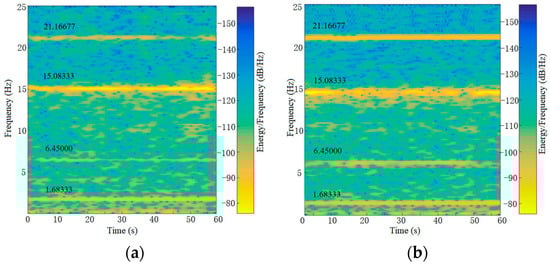
Figure 31. STFT recognition result of measurement point No.1. (a) Wireless; (b) Wired.

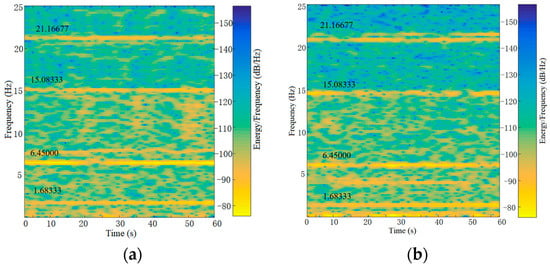
Figure 32. STFT recognition result of measurement point No.2. (a) Wireless; (b) Wired.

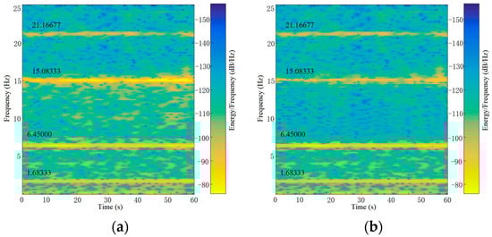
Figure 33. STFT recognition result of measurement point No.3. (a) Wireless; (b) Wired.

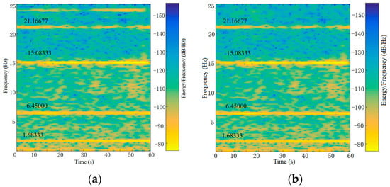
Figure 34. STFT recognition result of measurement point No.4. (a) Wireless; (b) Wired.

5.2.3. Wavelet Transform (WT)

WT is considered as a Fourier transform with adjustable windows, which can adaptively adjust the time and frequency length of the signal. The WT solves the defects in the STFT process, improves the characteristics of the time–frequency window, and solves the problems of frequency and time resolution aliasing in the analysis process. The process involves adding mother wavelets and sub wavelets to the Fourier transform, and the sub wavelets are obtained by scaling and translating the mother wavelet. Then, the signal is decomposed, and structural parameters are identified. If the signal is $f\left(t\right)\in L^2\left(R\right)$, then the WT is

$$W{T}_{\psi }\left(a,b\right)=\left[{\psi }_{\left(t\right)},{\phi }_{a,b}\left(t\right)\right]=\frac{1}{\sqrt{\left|a\right|}}{\displaystyle {\int }_{-\infty }^{+\infty }\psi \left(t\right)}\dot{\phi }\left(\frac{t-b}{a}\right)dt.$$

(5)

The convolution expression is:

$$W{T}_{\psi }\left(a,b\right)=\left[\psi \left(t\right),{\phi }_{a,b}\left(t\right)\right]=\frac{1}{\sqrt{\left|a\right|}}{\displaystyle {\int }_{-\infty }^{+\infty }\psi }\left(t\right)\phi \left(\frac{t-b}{a}\right)dt={\left|a\right|}^{\raisebox{1ex}{$1$}\!\left/ \!\raisebox{-1ex}{$2$}\right.}\dot{\psi }{\overline{\phi }}_{\left|a\right|}\left(b\right)$$

(6)

In the above expression:

• ${\overline{\phi }}_{\left|a\right|}\left(t\right)={\left|a\right|}^{-1}\dot{\phi }\left(\raisebox{1ex}{$-t$}\!\left/ \!\raisebox{-1ex}{$a$}\right.\right)$
• a—scale facto r(a > 0);
• b—shift factor (Can be positive or negative);
• $a,b,t\in R,a\ne 0.$
• $\phi \left(t\right)$—basic wavelet or mother wavelet, $\dot{\phi }\left(t\right)$ and $\phi \left(t\right)$ complex conjugate.

For the results of the pulsation test, take point 1 as an example for WT signal analysis, where the sampling frequency is 50 Hz, and the sampling time is 1 min. The test results are shown in Figure 35. During the sampling time, compared with the identification results of FFT and STFT, the WT identified the natural frequencies of the first three orders of the structure, and the distribution of the natural frequencies of the first three orders was basically consistent with the frequency distribution of FFT.

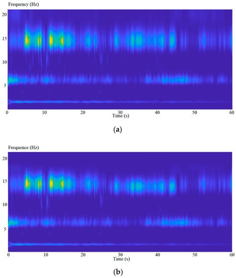
Figure 35. WT recognition result of measurement point No.1. (a) Wireless; (b) Wired.

5.3. Identification of Damping

5.3.1. Half-Power Bandwidth

Half-Power Bandwidth is the most commonly used frequency domain damping ratio identification method. Usually, the entire modal analysis is completed in conjunction with the peak picking method. After obtaining the frequency response function of the structure, the frequency corresponding to the peak point of the spectral line is the natural frequency of the structure. At the peak value of 0.707, draw a horizontal line, and the two points intersecting the spectral line are called half-power points (as shown in Figure 36). The damping ratio corresponding to the natural frequency of the structure at the peak value ξ’s expression for the half-power bandwidth of:

$$\xi =\frac{{\omega }_2-{\omega }_1}{2\omega }\frac{\Delta \omega }{2\omega }$$

(7)

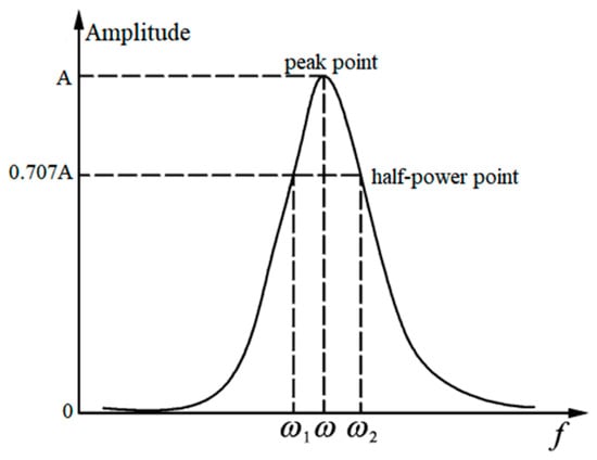
Figure 36. Schematic diagram of half-power bandwidth method.

• ω₁, ω₂: frequency value corresponding to half-power bandwidth point;
• ω: the frequency value corresponding to the peak point.

The traditional half-power bandwidth method for damping estimation does not consider the influence of higher-order terms. When calculating the second- and third-order damping ratio results, in order to eliminate the influence of different damping ratios between vibration modes on the calculation results, calculate the damping ratio of the second and third order modes using the extended Rayleigh damping model, and its expression is as follows:

$$\left[C\right]=a_0\left[M\right]+a_1\left[K\right]$$

(8)

In the above equation, a₀ and a₁ represent proportional coefficients. If the damping of the structure meets orthogonal conditions, the orthogonal conditions can be used to determine the coefficients a₀ and a₁.

Substitute the formula $C_n=2{\xi }_n{\omega }_n{M}_n$ ${\omega }_n{}^2=K_n/M_n$ into Equation (8) to obtain:

$${\xi }_n=\frac{a_0}{2{\omega }_n}+\frac{a_1{\omega }_n}{2}$$

(9)

ξ_n: damping ratio coefficient; ω_n: undamped natural frequency.

Based on the frequency domain results of measurement point 1 in Figure 16, the first three-order damping ratios of wireless and wired are calculated, and the results are shown in Table 10.

Table 10. Comparison of damping identification results by half-power bandwidth method.

Vibration Mode	Wireless Test Results		Wired Test Results
	Frequency (Hz)	Damping Ratio	Frequency (Hz)	Damping Ratio
first order	1.533840	0.04812463	1.533840	0.04825478
second order	6.118710	0.04825483	6.118710	0.04836279
third order	14.93831	0.10202145	14.93831	0.10229736

5.3.2. Logarithmic Decrement

The damping analysis method of logarithmic decay rate considers a single degree of freedom linear system:

$$\ddot{x}+2\xi {\omega }_n\dot{x}+{\omega }^{2}x=0$$

(10)

Free attenuation acceleration response:

$$x\left(t\right)=C{e}^{-\xi {\omega }_{n}t}\sin \left({\omega }_{d}t+\phi \right)$$

(11)

In the above expression:

• $\xi$—Damping ratio coefficient
• ${\omega }_n$—Undamped natural frequency
• ${\omega }_d={\omega }_n\sqrt{1-{\xi }^2}$—Damped natural frequency
• $C,\phi$—Constant determined by initial conditions

$$x\left(0\right)=C\sin \phi ,\dot{x}\left(0\right)=-C\xi {\omega }_n\sin \phi +C{\omega }_d\cos \phi$$

(12)

The logarithmic decay rate is:

$$\delta =\ln \frac{C_1}{C_2}=\ln \frac{C{e}^{-\xi {\omega }_n{t}_i}}{C{e}^{-\xi {\omega }_n\left(t_i+n{T}_d\right)}}=\xi {\omega }_n{T}_{d}n=2n\pi \xi /\sqrt{1-{\xi }^2}$$

(13)

In the above expression: $T_d=\frac{2\pi }{{\omega }_d}$—natural cycle, the damping coefficient can be calculated from the above formula.

Take some time history data from point 1 in Figure 15 and calculate the damping ratio of the wireless and wired test results using the logarithmic decay rate. The calculation results are shown in Table 11, and the time history data of the wired and wireless parts intercepted are shown in Figure 37. The damping ratios of wireless vibration sensors and wired acceleration sensors obtained by the half-power bandwidth method and logarithmic decay rate method are basically consistent.

Table 11. Comparison of damping ratio results for logarithmic decay rate identification.

Wireless Testing	Wired Testing
0.047	0.048

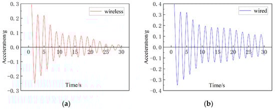
Figure 37. Part of the captured wireless test data (a) and wired test data (b).

5.4. Identification of Vibration Modes

The results of using wavelet transform to identify structural modal vibration modes are shown in Figure 38, Figure 39, Figure 40 and Figure 41. From the result identification graph, it can be seen that the vibration mode coefficients of the wireless vibration sensor and the wired acceleration sensor obtained by wavelet transform are basically consistent, and the trend in the vibration mode coefficients of the wired and wireless results is basically consistent with the height change.

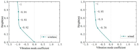
Figure 38. First-order mode diagram of wireless and wired test results.

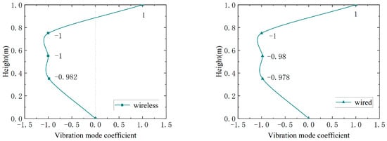
Figure 39. Second-order mode diagram of wireless and wired test results.

Figure 40. Third-order mode diagram of wireless and wired test results.

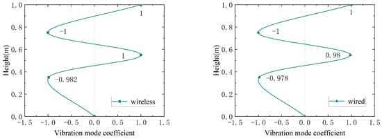
Figure 41. Fourth-order mode diagram of wireless and wired test results.

5.5. Field Vibration Test

In the top floor of the clock tower located in Dalian University, a wireless vibration sensor and a wired acceleration sensor were used for field vibration test (as shown in Figure 42). During the sampling process, the sampling rates of both the wireless vibration sensor and the wired acceleration sensor was set to 50 Hz. Data from the same time period and a duration of 1 min during the sampling process were selected for analysis, and the time history and frequency domain curves shown in Figure 43 and Figure 44 were obtained.

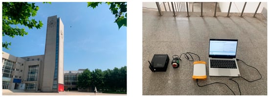
Figure 42. Field vibration test.

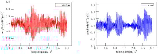
Figure 43. Time history curves of wireless and wired under field vibration test.

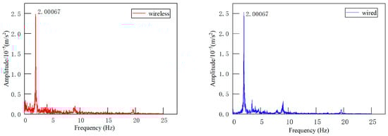
Figure 44. Frequency domains diagram of wireless and wired under field vibration test.

From Figure 43, it can be seen that the self-noise levels of the wireless vibration sensors were higher than those of the wired acceleration sensors, but they met the monitoring requirements in earthquake monitoring and health monitoring of civil engineering structures. From Figure 44, it can be seen that the natural frequencies of the structure obtained by the wireless vibration sensor and the wired acceleration sensor were consistent, and the noise level of the low-frequency wireless vibration sensor was higher than that of the wired acceleration sensor. However, in the frequency band greater than 1 Hz, the difference between the two was not significant, and the measurement accuracy met the requirements of engineering monitoring.

6. Conclusions

(1)

Using FFT, STFT, and WT to identify the natural frequency of experimental data, the FFT identification results of the free attenuation test showed that the first three orders of the natural frequency identification results of the wireless and wired test points were consistent. In the FFT identification results of the pulsation test, the first four natural frequencies of each measurement point in the wireless and wired tests were consistent; however, the first three order identification results of the pulsation test were larger than the free attenuation identification results. The reason for the error may have been the shaking of the model structure during the free attenuation test, which caused damage to the internal components of the structure.

(2)

The changes in the first four, three, and order natural frequencies of the structure in the time domain were identified using STFT and WT, respectively. The identification results were basically consistent with the frequency distribution in the FFT.

(3)

The frequency domain and time domain data of point 1 in the free attenuation test were calculated using the half-power bandwidth method and the logarithmic attenuation method, and the damping ratio results of the structure were basically consistent.

(4)

The vibration mode recognition results of the wired and wireless test data during the wavelet transform were basically consistent.

(5)

The field vibration test results of wireless and wired methods showed that the natural frequencies of the structure obtained by the two methods were consistent, and, in the low frequency range, the noise level of the wireless testing was higher than that of wired testing, but the difference between the two was small in the frequency band above 1 Hz.

The above test data fully proved the accuracy and reliability of the wireless vibration sensor test data capabilities and also proved the accuracy of the time–frequency analysis method program developed in this paper to identify structural dynamic characteristic parameters. Therefore, the wireless vibration sensor could be used in the field of civil engineering Structural Health Monitoring.

References

- Mesquita, E.; Arede, A.; Pinto, N.; Antunes, P.; Varum, H. Long-term monitoring of a damaged historic structure using a wireless sensor network. Eng. Struct. 2018, 161, 108–117. [Google Scholar] [CrossRef]
- Alejandro, M.G.; Carlos, A.P.R.; Aurelio, D.G.; Martin, V.R.; Omar, C.A.; Juan, P.A.S. Sensors Used in Structural Health Monitoring. Arch. Comput. Methods Eng. 2018, 25, 901–918. [Google Scholar] [CrossRef]
- Wu, R.T.; Jahanshahi, M.R. Data fusion approaches for structural health monitoring and system identification: Past, present, and future. Struct. Health Monit.-Int. J. 2020, 19, 552–586. [Google Scholar] [CrossRef]
- Guo, J.Q.; Xie, X.B.; Bie, R.F.; Sun, L.M. Structural health monitoring by using a sparse coding-based deep learning algorithm with wireless sensor networks. Pers. Ubiquitous Comput. 2014, 18, 1977–1987. [Google Scholar] [CrossRef]
- Zhang, Y.; Kim, C.W.; Zhang, L.; Bai, Y.T.; Yang, H.; Xu, X.Y.; Zhang, Z.H. Long term structural health monitoring for old deteriorated bridges: A copula-ARMA approach. Smart Struct. Syst. 2020, 25, 285–299. [Google Scholar] [CrossRef]
- Ma, H.Y.; Li, J.; Su, X.Y.; Han, Y.; Pang, K.; Sun, Z.P. Design of bridge all-weather health monitoring system based on wireless sensor network. Foreign Electron. Meas. Technol. 2021, 40, 150–155. (In Chinese) [Google Scholar]
- Ye, F.Y.; Wang, X.C. Dam safe monitoring information management and application. Electron. Meas. Technol. 2018, 41, 75–79. (In Chinese) [Google Scholar]
- Liu, F.; Wang, Q.; Yang, Y.; Xu, W.J. Study of accelerometer-based vibration monitoring of high rise building. Transducer Microsyst. Technol. 2020, 39, 36–39. (In Chinese) [Google Scholar]
- Zhao, L.; Zhang, T.; Huang, X.B.; Zhang, Y.; Liu, W. A structural health monitoring system of the overhead transmission line conductor. Iet Sci. Meas. Technol. 2021, 16, 28–39. [Google Scholar] [CrossRef]
- Annamdas, V.G.M.; Bhalla, S.; Soh, C.K. Applications of structural health monitoring technology in Asia. Struct. Health Monotoring—Int. J. 2017, 16, 324–346. [Google Scholar] [CrossRef]
- Guemes, A.; Salowitz, N.; Chang, F.K. Trends on research in structural health monitoring. Struct. Health Monotoring—Int. J. 2014, 13, 579–580. [Google Scholar] [CrossRef]
- Padmavathy, T.V.; Bhargava, D.S.; Venkatesh, P.; Sivakumar, N. Design and development of microstrip patch antenna with circular and rectangular slot for structural health monitoring. Pers. Ubiquitous Comput. 2018, 22, 883–893. [Google Scholar] [CrossRef]
- Sivasuriyan, A.; Vijayan, D.S.; Leemarose, A.; Revathy, J.; Monicka, S.G.; Adithya, U.R.; Daniel, J.J. Development of Smart Sensing Technology Approaches in Structural Health Monitoring of Bridge Structures. Adv. Mater. Sci. Eng. 2021, 2021, 2615029. [Google Scholar] [CrossRef]
- Omar, S.S.; Muhammad, R. Algorithms and Techniques for the Structural Health Monitoring of Bridges: Systematic Literature Review. Sensors 2023, 23, 4230. [Google Scholar] [CrossRef]
- Abdelgawad, A.; Yelamarthi, K. Internet of Things (IoT) platform for structure health monitoring. Wirel. Commun. Mob. Comput. 2017, 2017, 6560797. [Google Scholar] [CrossRef]
- Chowdhry, B.S.; Shah, A.A.; Uqaili, M.A.; Memon, T. Development of IOT Based Smart Instrumentation for the Real Time Structural Health Monitoring. Wirel. Pers. Commun. 2020, 113, 1641–1649. [Google Scholar] [CrossRef]
- Zhang, M.C.; Liu, Z.T.; Shen, C.; Wu, J.B.; Zhao, A. A Review of Radio Frequency Identification Sensing Systems for Structural Health Monitoring. Materials 2022, 15, 7851. [Google Scholar] [CrossRef]
- Yan, S.; Ma, H.Y.; Li, P.; Song, G.B.; Wu, J.X. Development and Application of a Structural Health Monitoring System Based on Wireless Smart Aggregates. Sensors 2017, 17, 1641. [Google Scholar] [CrossRef]
- Shi, Y.; Ma, H.Y.; Jiang, X.L.; Qi, B.H.; Liu, F.X. A Bridge Health Monitoring System Based on Wireless Smart Aggregates. Appl. Mech. Mater. 2014, 578–579, 1138–1144. [Google Scholar] [CrossRef]
- Heo, G.; Son, B.; Kim, C.; Jeon, S.; Jeon, J. Development of a Wireless Unified-Maintenance System for the Structural Health Monitoring of Civil Structures. Sensors 2018, 18, 1485. [Google Scholar] [CrossRef]
- Vega, F.; Yu, W. Smartphone based structural health monitoring using deep neural networks. Sens. Actuators A-Phys. 2022, 346, 113820. [Google Scholar] [CrossRef]
- Han, R.C.; Zhao, X.F. Shaking Table Tests and Validation of Multi-Modal Sensing and Damage Detection Using Smartphones. Buildings 2021, 11, 477. [Google Scholar] [CrossRef]
- Ozer, E.; Feng, M.Q. Structural Reliability Estimation with Participatory Sensing and Mobile Cyber-Physical Structural Health Monitoring Systems. Appl. Sci. 2019, 9, 2840. [Google Scholar] [CrossRef]
- Li, X.F.; Xiao, Y.Y.; Guo, H.N.; Zhang, J.S. A BIM Based Approach for Structural Health Monitoring of Bridges. Ksce J. Civ. Eng. 2021, 26, 155–165. [Google Scholar] [CrossRef]
- Valinejadshoubi, M.; Bagchi, A.; Moselhi, O. Development of a BIM-Based Data Management System for Structural Health Monitoring with Application to Modular Buildings: Case Study. J. Comput. Civ. Eng. 2019, 33, 05019003. [Google Scholar] [CrossRef]
- Chandrasekaran, S.; Chithambaram, T. Health monitoring of tension leg platform using wireless sensor networking: Experimental investigations. J. Mar. Sci. Technol. 2019, 24, 60–72. [Google Scholar] [CrossRef]
- Kim, B.; Min, C.; Kim, H.; Cho, S.; Oh, J.; Ha, S.H.; Yi, J.H. Structural Health Monitoring with Sensor Data and Cosine Similarity for Multi-Damages. Sensors. 2019, 19, 3047. [Google Scholar] [CrossRef] [PubMed]
- Zhao, X.Y.; Lang, Z.Q. Baseline model based structural health monitoring method under varying environment. Renew. Energy 2019, 138, 1166–1175. [Google Scholar] [CrossRef]
- Buckley, T.; Ghosh, B.; Pakrashi, V. Edge Structural Health Monitoring (E-SHM) Using Low-Power Wireless Sensing. Sensors 2021, 21, 6760. [Google Scholar] [CrossRef] [PubMed]
- Zanelli, F.; Castelli-Dezza, F.; Tarsitano, D.; Mauri, M.; Bacci, M.L.; Diana, G. Design and Field Validation of a Low Power Wireless Sensor Node for Structural Health Monitoring. Sensors 2021, 21, 1050. [Google Scholar] [CrossRef] [PubMed]
- Li, C.H.; Teng, Y.T.; Zhou, J.C.; Hu, X.X.; Wang, X.Z.; Li, X.j.; Wang, Y.S. Design on high-precision time-synchronization system for distributed seismic data acquisition. Acta Seismol. Sin. 2022, 44, 1111–1120. (In Chinese) [Google Scholar]
- Sofi, A.; Regita, J.J.; Rane, B.; Lau, H.H. Structural health monitoring using wireless smart sensor network-an overview. Mech. Syst. Signal Process. 2021, 163, 108113. [Google Scholar] [CrossRef]
- Nvabiva, N.; Beskhyroun, S.; Matulish, J. Development of wireless smart sensor network for vibration-based structural health monitoring of civil structures. Struct. Infrastruct. Eng. 2022, 18, 345–361. [Google Scholar] [CrossRef]
- Gael, L.; Alassane, S.; Alexandru, T.; Daniela, D. Autonomous wireless sensors network for the implementation of a cyber-physical system monitoring reinforced concrete civil engineering structures. IFAC-PapersOnLine 2022, 55, 19–24. [Google Scholar] [CrossRef]
- Zhang, D.Y.; Tian, J.D.; Li, H. Design and Validation of Android Smartphone Based Wireless Structural Vibration Monitoring System. Sensors 2020, 20, 4799. [Google Scholar] [CrossRef]
- Morgenthal, G.; Eick, J.F.; Rau, S.; Taraben, J. Wireless Sensor Networks Composed of Standard Microcomputers and Smartphones for Applications in Structural Health Monitoring. Sensors 2019, 19, 2070. [Google Scholar] [CrossRef]
- Bai, H.D.; Li, S.; Barreiros, J.; Tu, Y.Q.; Pollock, C.R.; Shepherd, R.F. Stretchable distributed fiber-optic sensors. Science 2020, 370, 6518. [Google Scholar] [CrossRef] [PubMed]
- Bai, X.; Yang, M.J.; Ajmera, B. An Advanced Edge-Detection Method for Noncontact Structural Displacement Monitoring. Sensors 2020, 20, 4941. [Google Scholar] [CrossRef] [PubMed]
- Li, P.; Li, L.Y.; Song, G.B.; Yu, Y. Wireless sensing and vibration control with increased redundancy and robustness design. IEEE Trans. Cybern. 2014, 44, 2076–2087. [Google Scholar] [CrossRef]
- Yang, J.; Fan, T.; Huang, W.; Deng, T.; Yuan, Q. Development of engineering strong vibration accelerometer based on MEMS sensor. J. Nat. Disasters 2022, 31, 181–189. (In Chinese) [Google Scholar]
Disclaimer/Publisher’s Note: The statements, opinions and data contained in all publications are solely those of the individual author(s) and contributor(s) and not of MDPI and/or the editor(s). MDPI and/or the editor(s) disclaim responsibility for any injury to people or property resulting from any ideas, methods, instructions or products referred to in the content. |
© 2023 by the authors. Licensee MDPI, Basel, Switzerland. This article is an open access article distributed under the terms and conditions of the Creative Commons Attribution (CC BY) license (https://creativecommons.org/licenses/by/4.0/).