Analysis of the Sustainable Driving Effect of Building Energy Consumption on Economic Development Based on the Sustainable Driving Force Model

Abstract

The environmental problems caused by building energy consumption (BEC) are becoming increasingly prominent. Reducing building energy consumption can not only effectively curb environmental pollution, but also continue to promote economic development. However, there are few reports on reducing building energy consumption to continuously promote economic development. Sustainable driving force (SDF) has been widely mentioned in past research as a common-sense concept, but few systematic studies have been carried out. The main research objectives of this article include two aspects: On the one hand, this study takes the lead in establishing an SDF model and conducting systematic research on SDF. On the other hand, based on the SDF model, an empirical study is conducted on the sustainable driving effect of reducing building energy consumption on economic development in China. The main conclusions are as follows: (1) Research on the SDF model: Based on common examples, the objective reality of SDF has been theoretically proven. Based on the relevant theories of econometrics, this article believes that the “Granger causality test” and the “distributed lag regression model” can be used as basic tools for quantitative research of SDF models. (2) Research on the application of SDF model: From the Granger causality test, it can be seen that the current BEC intensity is the Granger cause of China’s economic development in the first and eighth cycles of the future. According to the results of the distributed lag regression model, reducing BEC intensity has a sustainable driving effect on economic development. Specifically, in the lagged period 1~8, the sustainable driving effect (reverse effect) of BEC on economic development gradually increases at first (coefficient value from 3878.52 to 5163.87), and then gradually decreases (coefficient value from 5163.87 to 783.534). To sum up, the SDF model can provide a reference for the quantitative study of SDF; studying the sustainable driving effect of BEC on economic development can provide a macro reference for the government to formulate “energy conservation and emission reduction” measures.

1. Introduction

In recent years, the activities of the construction industry and residents have accounted for approximately 30% to 40% of the global final energy consumption, but this figure may vary by country and time period [1,2,3]. In the United States, the energy consumption of the construction sector accounts for 39% of the total energy consumption, while the energy consumption of residential buildings in the European Union accounts for approximately 40% of the total BEC [4,5]. Such huge energy consumption in the construction industry makes carbon emissions increasingly serious, which is the cause of global warming, climate change and air pollution [6]. Driven by technological and industrial development, population growth and the need to improve living standards, the rising of BEC cannot be curbed easily [7]. 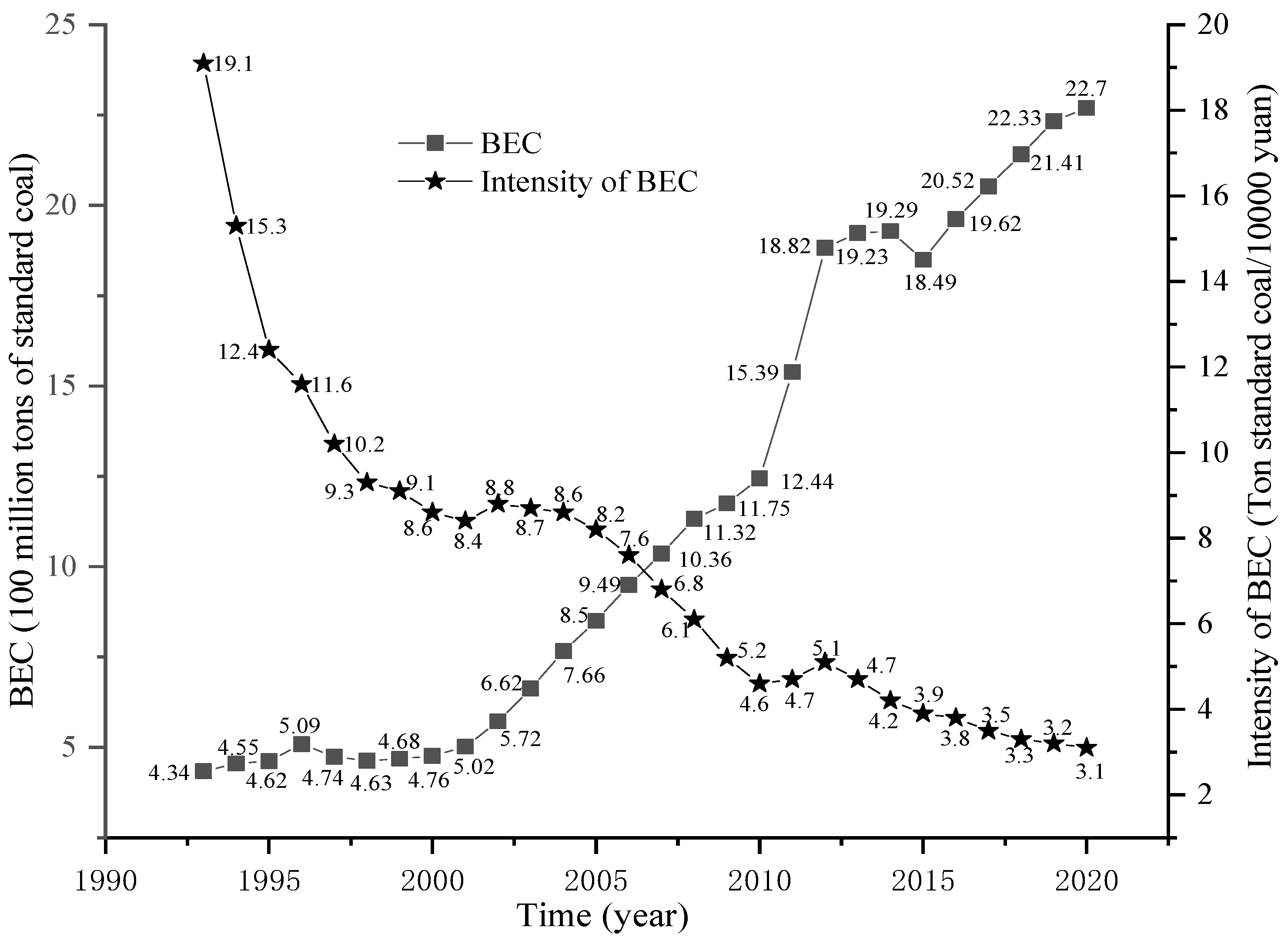The UNEP-SBCI report, Building and Climate Change: Summary for decision-maker, (the United Nations Environment Programme-Sustainable Building & Climate Initiative), highlights that BEC accounts for 40% of global energy consumption, and 1/3 of global greenhouse gas emissions are related to buildings [8]. Over the years, the BEC in China has been on the rise. The total energy consumption of buildings nationwide has reached 899 million tons of standard coal, with public buildings accounting for 38.53% of the energy consumption [9]. At present, the consumption structure of urban and rural residents in China has gradually upgraded from “clothing and food” to “living and transportation”; the goal of life has changed from survival to comfort. China’s urban and rural residents’ requirements for living conditions such as building areas, indoor environment comfort and so on are gradually increasing, resulting in a continuous rise in BEC, which will become the main growth point of energy consumption and CO₂ emissions in the next 20 years. In the “Outline of the 13th Five-Year Plan for Housing and Urban-Rural Development”, the Chinese government clearly highlights the need to “develop green buildings, green building materials, and vigorously strengthen building energy conservation”. Meanwhile, it clearly requires that by 2020, the proportion of green building promotion in new urban buildings will exceed 50%, the proportion of green building materials application will exceed 40% and the energy efficiency requirements of new buildings will be 20% higher than the end of the 12th Five-Year Plan [10].

The continuous rise of BEC has attracted the attention of many scholars at home and abroad. Due to the lack of detailed data on BEC, some scholars have carried out data calculation research in this area [11,12,13]. For example, Zhuang et al. (2011) calculated the energy consumption of urban civil buildings based on statistical yearbooks, energy balance tables, and sampling survey data. The results showed that the building energy consumption obtained by these three methods can be mutually referenced and verified, and can be used to calculate the energy consumption of urban civil buildings [12]. Other scholars have begun to adopt new technologies based on artificial intelligence, machine learning, the Internet of Things, edge and cloud computing to promote building energy efficiency [6]. In addition, multiple studies have focused on BEC prediction models [14,15], because prediction models play an indispensable role in energy management and conservation [16]. There are also references related to the relationship between energy consumption and economic development. In the context of China’s rapid economic development, the BEC has increased sharply. Reducing the BEC can further accelerate the building of a resource-saving and environmentally friendly society [17]. Energy consumption and economic growth have a two-way causal relationship; China’s energy consumption is positively correlated with economic growth [18]. In China, energy consumption, energy use and energy import are positively related to economic development [19]. Based on the analysis of the economic development and energy consumption status in Guangdong Province, Zhang [20] selects the corresponding variables and conducts a co-integration analysis and Granger causality test, further constructing the VAR model of impulse response analysis to study the relationship between energy consumption and economic growth. In China, there is a long-term and stable relationship between energy consumption and economic growth, and there is a one-way causal relationship between economic growth and energy consumption [21]. Huo [22] innovatively develops the Integrated Dynamic Emission Assessment Model (IDEAM) to model the dynamic evolution of Chinese commercial building carbon emissions toward 2060. The results show that commercial building carbon emissions will peak at 1.28 Gigatons (Gt) of CO₂ in 2037 under the baseline scenario and will advance toward 2029 with an emissions peak of 0.98 Gt CO₂ under the low-carbon scenario. The study provides a deeper understanding of possible emission pathways.

The foresaid research literature can be summarized as follows: Firstly, BEC accounts for a large proportion of total energy consumption, resulting in increasingly prominent environmental problems. Reducing BEC is an important issue to be urgently solved. Secondly, with the development of the social economy, people’s demand for housing is increasing, and the development of the construction industry has become an important part of economic development. Thirdly, from the perspective of economic development, energy consumption plays a positive role in promoting economic development.

From the perspective of the current complex trend of global economic development, reducing BEC contains rich content: reducing the consumption of fossil energy can effectively curb environmental problems [7]; reducing BEC can force the development and utilization of green energy [23]; reducing energy consumption can promote the upgrading of industrial structure [13] and so on. Therefore, this paper believes that reducing BEC is to promote sustainable economic development. However, there are few reports on the sustainable driving effect of reducing BEC on economic development.

In the existing research literature, although the expression is different, there are many references related to SDF. When examining the reproduction of social capital, Marx first clearly put forward the concept of SDF. Marx believed that monetary capital is the first driving force to launch the entire process of capitalist production. Capital in monetary form, or monetary capital as the first driving force and SDF of every new enterprise, whether it is a social investigation or individual investigation, is the requirement for the production of capitalist commodities [24]. The existing research literature has demonstrated that there are a large number of entries on continued impetus or SDF. In web of science, 16,934 results are displayed if you enter the topic (impetus) [25,26,27,28], for the topic (driving force), 174,578 results are displayed [29,30,31,32,33] and for the topic (sustainability), 247,548 results are displayed [34,35,36]. Whether in natural or social sciences, it has been found that the terms “impetus”, “driving force” and “sustainability” are frequently used. For example, many articles directly use the terms “impetus”, “driving force” and “sustainability” in the title [37,38,39,40,41,42].

For the convenience of research, the following discussion combines the relevant research on sustainability into “sustainable driving force”. In summary, the above studies are based on the basic assumption that SDF is a common-sense term. There are many direct or indirect qualitative or quantitative descriptions of SDF, but there is a lack of systematic quantitative research. There are a large number of references confirming this conclusion. When studying sustainable agriculture, Cui [43] points out that scientific development and technological progress are the key driving forces of agricultural transformation. Chang [39] analyzes the dynamic changes and driving forces of urbanization in Xi’an from 1997 to 2016, and finds that topographic factors, policies and geographical location are the main driving forces of land use and urbanization change. Hou [44] believes that the information and communication technology supported by the Internet has become an important driving force to promote the intelligent development of China’s environmental governance. Zhao [45] conducts an empirical study on the relationship between China’s education level and economic development from 1978 to 2005 by using the distributed lag regression model and Granger causality test; the results show that China’s education level has a strong SDF for economic development. From the perspective of time and space, SDF is a concept of time dimension, and the difficulty for the research on SDF is its existence and occurrence conditions. This paper takes the above discussion as the logical starting point of the study, and carries out the following research. Firstly, based on a common example, this paper theoretically verifies the existence and occurrence conditions of SDF. Secondly, the Granger causality test can test whether one group of time series is the cause of change of another group of time series in a statistical sense; the distributed lag regression model can judge the impact of each lagged value of the independent variable on the dependent variable by the significance test of the coefficient of the regression equation. Therefore, with the help of Granger causality test and the distributed lag regression model in econometrics, the systematic quantitative study of SDF can be carried out. Finally, a study on the sustainable driving role of BEC on China’s economic development by using the quantitative research method of SDF is conducted. The innovations of this article are the following two points: (1) This study takes the lead in establishing an SDF model and proves its objective reality based on common cases; and (2) With the help of econometrics, the method of quantitative research on SDF is systematically explored.

In brief, the main aim of this article includes two aspects: (1) This study takes the lead in establishing an SDF model and conducted systematic research on SDF. (2) Based on the SDF model, an empirical study is conducted on the sustainable driving effect of reducing building energy consumption on China’s economic development.

2. Objective Reality of SDF

At present, there is no systematic study on SDF of one time-series variable X on another time series variable X. This research will theoretically verify the existence and the occurrence conditions of SDF based on a common case.

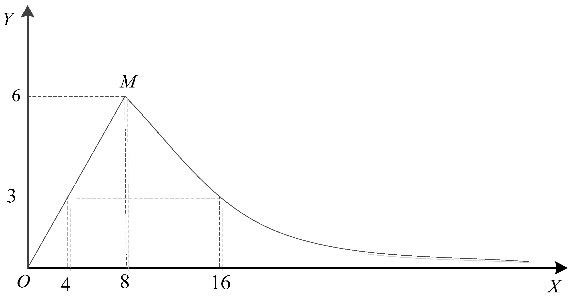
Example illustration: In order to prevent “influenza,” a school disinfects its classrooms by fumigation. It is known that during the combustion of drugs, the drug’s content X (mg) per cubic meter in the air of the classroom is in positive proportion to the time X (min), and after the combustion of drugs, X is in inverse proportion to the time X. Now, it is measured that the drugs can be burned within 8 min; the drug’s content per cubic meter in the classroom air is 6 mg when the combustion is completed. Moreover, medical studies have shown that the drug is only effective if the amount of it in the air is at least 3 mg per cubic meter. Therefore, how many minutes is the effective time for the fumigation and disinfection of drugs (This example is a common function exercise in middle school teaching in China)? The answer to the example is obvious, and the expression of its function is as follows:

$$y=\left\{\begin{array}{ll}\frac{3}{4}x& (0\le x<8)\\ \frac{48}{x}& (x\ge 8)\end{array}\right.$$

(1)

When the drug’s content y is 3 mg, as shown in Figure 1, the intersection coordinates are obtained by the simultaneous Equation (1). It can be seen that the drug’s content per cubic meter in the air in the classroom is more than 3 mg between the 4th minute and the 16th minute from Figure 1. Furthermore, we can get the result of the example; that is, the effective time of the fumigation is 12 min.

If it takes more than 12 min to meet the requirements of fumigation, the drug must be put in again at a certain time point for fumigation. After that, it is necessary to put drugs into fumigation many times to continuously meet the requirements of fumigation. In general, meeting the current fumigation requirements depends not only on the current drug investment, but also on the previous drug investment. Namely, satisfying the current fumigation conditions is the result of the superposition of the current drug input and the previous drug input, and the previous drug input has a sustainable driving effect on the current fumigation results. The above drug investment can be divided into two cases: non-periodic investment and periodic investment. The objective reality and occurrence conditions of SDF in the above two cases are studied below.

2.1. Non-Periodic Investment of Fumigation

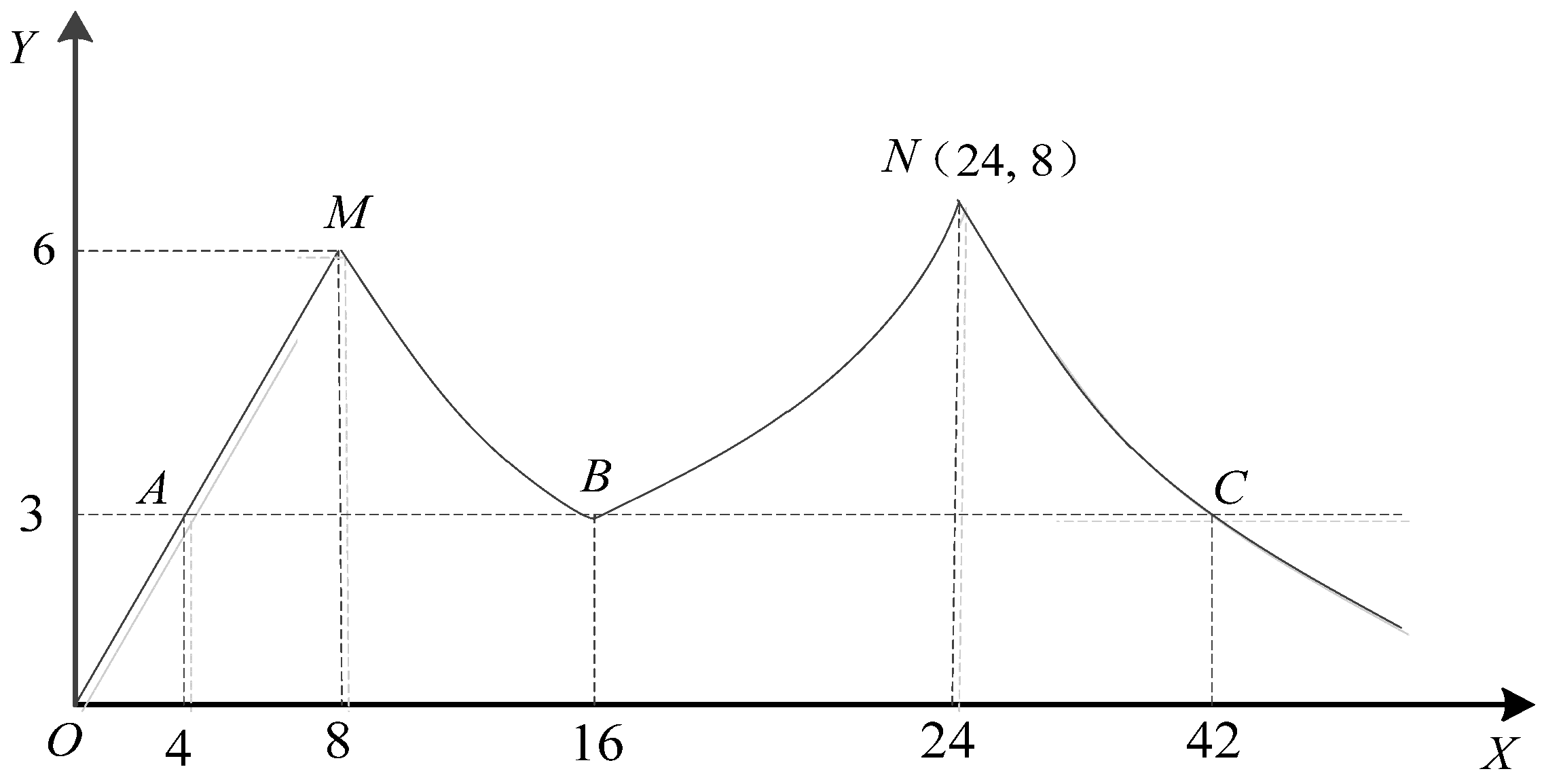
If the standard of fumigation and disinfection remains unchanged; that is, the drug’s content per cubic meter in the air in the teaching room is not less than 3 mg, it is assumed that the intensity of fumigation and disinfection of each phase is similar, and that the fumigated drugs in each phase were burned within 8 min. If the effective time of fumigation and disinfection needs to be extended, the second phase, the third phase and even more phases of the drug’s fumigation will be required. In order to ensure the sustainability of the effective time of the drug’s fumigation and disinfection, the start time of the fumigation and disinfection of the drugs in period 2 will be set as the 16th minute of the fumigation and disinfection in period 1 (Figure 2). Considering the drug’s effect in period 1 of fumigation and disinfection after 16 min, the functional expression of period 2 of the fumigation and disinfection of the drugs can be obtained as follows:

$$y=\left\{\begin{array}{ll}\frac{3}{4}x-12+\frac{48}{x}& (16\le x<24)\\ \frac{48}{x}+\frac{48}{x-16}& (x\ge 24)\end{array}\right.$$

(2)

When the drug’s content y is 3 mg, as shown in Figure 2, the intersection coordinates are obtained by the simultaneous Equation (2). According to the above calculation, between the 16th and the 42nd minute, the drug’s content per cubic meter in the air in the classroom shall not be less than 3 mg. It can be further demonstrated that the effective time of fumigation is 26 min. The investment in the second phase is the same as that in the first phase, but the effective time of the drug’s fumigation is 14 min longer than that in the first phase. At the same time, from Equations (1) and (2), the contribution of investment (48/x) in the first phase to the fumigation continues to the second phase, indicating that the investment in the early stage has a continuous promoting effect on the current fumigation effect.

Similarly, the start time of the third phase of the fumigation and disinfection of the drugs is set as the 42nd minute (Figure 2). Considering the drug’s action in the first phase and the second phase of fumigation and disinfection after 42 min, the functional expression of the third phase of fumigation and disinfection can be obtained as follows:

$$y=\left\{\begin{array}{ll}\frac{3}{4}x-\frac{63}{2}+\frac{48}{x}+\frac{48}{x-16}& (42\le x<50)\\ \frac{48}{x}+\frac{48}{x-16}+\frac{48}{x-42}& (x\ge 50)\end{array}\right.$$

(3)

This shows that Equation (3) is a monotone increasing function in the interval [42, 50) and a monotone decreasing function in the interval [50, +∞). When the drug’s content y is 3 mg, the intersection coordinates are obtained by the simultaneous Equation (3). Furthermore, it can be found that the effective time of period 3 of fumigation and disinfection is 31 min. Similarly, the effective time of the fumigation and disinfection of the drugs in period 4 or even further can be calculated. In Equations (1)–(3), there is a common term (48/x), which indicates that the drug input in the first phase has a continuous promoting effect on the drug’s smoking effect in the second and third phases. The common term (48/(x − 16)) in Equations (2) and (3) shows that the drug input in the second phase has a continuous promoting effect on the drug fumigation effect in the third phase.

2.2. Periodic Investment of Fumigation

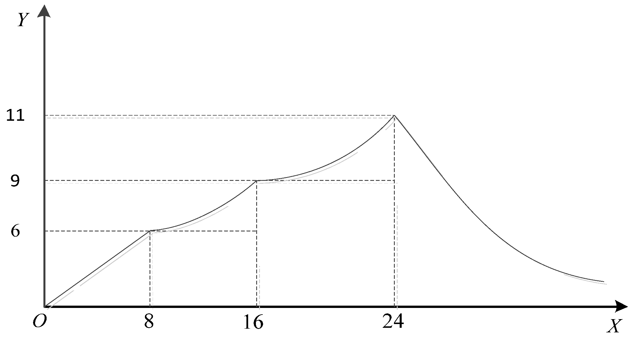
If the standard of the fumigation and disinfection of the drugs changes; that is, from the 8th minute, the drug’s content per cubic meter in the air needs to be steadily increased to enhance the effectiveness of the fumigation and disinfection, its cost also needs to be considered. After repeated research and trial calculation, and considering the characteristics of the fumigation and disinfection of the drugs in the example, the investment of fumigation and disinfection should meet the above requirements in Phases 1, 2, 3 or even more phases with the time cycle of 8 min. Considering the superposition effect of the three stages of fumigation and disinfection, the function expression (4) and the corresponding function image (Figure 3) of the fumigation and disinfection of the drugs can be obtained, whose function expression is as follows:

$$y=\left\{\begin{array}{l}\frac{3}{4}x(0\le x<8)\\ \frac{3}{4}x-6+\frac{48}{x}(8\le x<16)\\ \frac{3}{4}x-12+\frac{48}{x}+\frac{48}{x-8}(16\le x<24)\\ \frac{48}{x}+\frac{48}{x-8}+\frac{48}{x-16}(x\ge 24)\end{array}\right.$$

(4)

It has been further demonstrated that if the investment of the continuous intensity is still carried out in the cycle of 8 min after 24 min, the function image will change periodically in the state of 8 min to 24 min as shown in Figure 3. In addition, under the condition of ensuring the effectiveness of the fumigation and disinfection of the drugs, this cyclical continuous investment will lead to a steady increase of the drug’s content per cubic meter in the air in the classroom.

The common term (48/x) in Equation (4) shows that the drug input in the first phase has a continuous promoting effect on the drug fumigation effect in the second and third phases. The common term (48/(x − 8)) in Equation (4) shows that the drug input in the second phase has a continuous promoting effect on the drug fumigation effect in the third phase.

3. Methodology

The aforementioned theoretical research proves the existence and occurrence conditions of SDF. Further study shows that the quantitative research methods of SDF are contained in econometrics, which needs in-depth study. Sims (1980) introduces the VAR model (variable autoregressive model) into economics, which promotes the widespread application of the dynamic analysis of the economic system [46]. The VAR model is usually used to predict interconnected time-series systems and analyze the dynamic impact of random perturbations on variable systems to explain the impact of various economic shocks on the formation of economic variables. This study implies a continuous driving effect, but it does not mention the relevant issues of SDF. Another important application of the VAR model is to analyze the causal relationship between time-series variables. This theory is proposed by Granger [47], and its main content can be expressed as follows: whether variable X is the Granger cause of variable X mainly depends on the extent to which current variable X can be explained by past variable X; that is, whether adding some lag variable values of variable X can significantly improve the degree of interpretation to variable X. Sims proposes and proves a theorem convenient for the Granger causality test, which greatly promotes its wide application in economics [48].

3.1. From the Perspective of Granger Causality Test

To study whether variable X is the Granger cause of variable X, the steps are as follows:

(1)

Establish the regression equation:

$$Y_t=\sum _{i=1}^m{\alpha }_i{X}_{t-i}+\sum _{i=1}^m{\beta }_i{Y}_{t-i}+{\mu }_t$$

(5)

(2)

Suggest a hypothesis: ① Original hypothesis H₀: Variable X is not the Granger cause of variable X; that is, α₁ = α₂ = … = α_m = 0; ② Alternative hypothesis H₁: Variable X is the Granger cause of variable X; that is, α₁, α₂, …, α_m are not all 0.

(3)

Construe statistics: Make regressions (unconstrained regression and constrained regression) including and excluding the lag term of variable X for Equation (5), and record the sum of squares of the residuals of the former as RSS_U and the sum of squares of residuals of the latter as RSS_R; then we can construct F-statistics.

$$F=\frac{\left(RS{S}_R-RS{S}_U\right)/m}{RS{S}_U/\left(n-k\right)}$$

(6)

Here, m is the number of lag terms of variable X, n is the number of observations and k is the number of parameters to be estimated in the unconstrained regression. If the calculated F-statistic is greater than the critical value F_α (m, n − k) at a given significance level, the original hypothesis H₀ is rejected; that is, variable X is the Granger cause of variable X. Similarly, we can study whether variable X is the Granger cause of variable X. In the Granger causality test, in order to further study the continuous effect of an early input on the current output, if we take m = 1, 2, 3, 4 (lags: 1, 2, 3, 4) as an example, we can get Equations (7)–(10).

$$Y_t={\alpha }_1{X}_{t-1}+{\beta }_1{Y}_{t-1}+{\mu }_t$$

(7)

$$Y_t={\alpha }_1{X}_{t-1}+{\alpha }_2{X}_{t-2}+{\beta }_1{Y}_{t-1}+{\beta }_2{Y}_{t-2}+{\mu }_t$$

(8)

$$Y_t={\alpha }_1{X}_{t-1}+{\alpha }_2{X}_{t-2}+{\alpha }_3{X}_{t-3}+{\beta }_1{Y}_{t-1}+{\beta }_2{Y}_{t-2}+{\beta }_3{Y}_{t-3}+{\mu }_t$$

(9)

$$Y_t={\alpha }_1{X}_{t-1}+{\alpha }_2{X}_{t-2}+{\alpha }_3{X}_{t-3}+{\alpha }_4{X}_{t-4}+{\beta }_1{Y}_{t-1}+{\beta }_2{Y}_{t-2}+{\beta }_3{Y}_{t-3}+{\beta }_4{Y}_{t-4}+{\mu }_t$$

(10)

In Equation (7), when passing the F-test, it means that the coefficient α₁ ≠ 0, which indicates that the previous input of the variable X has a continuous driving effect on the current output Y, or that the current output Y is determined by the previous input of the variable X and the previous output Y. Namely, variable X is the Granger cause of variable X. On the contrary, when passing the F-test, it means that variable X is not the Granger cause of variable Y. Namely, the previous input of the variable X does not have a sustainable driving effect on the current output Y. In Equation (8), when passing the F-test, if the coefficient α₁ and α₂ are not all 0, it means that variable X is the Granger cause of variable X. On the contrary, when passing the F-test, it means that variable X is not the Granger cause of variable Y. Similarly, in Equations (9) and (10), there are similar conclusions.

From the above analysis, it is easy to get the following results: in the case of setting a lag period, there is a lag period in which the F-test is passed, and we can determine that variable X has a sustainable driving effect on variable X. Otherwise, the conclusion does not hold.

3.2. From the Perspective of the Distributed Lag Regression Model

In the Granger causality test, the research on SDF has the following defects: (a) taking into account time, some economic variables are essentially continuous time stochastic processes, and the observed time series data can only be regarded as a sample of the real variable continuous time process. Sims has proved that there is no necessary correspondence between Granger causality in continuous time and Granger causality in discrete time. Specifically, although it is inferred from the observed time-series data that variable X is the Granger cause of variable X, the fact may be that variable X is not the Granger cause of variable X [49]; (b) We can only judge whether variable X has a continuous driving effect on variable X under the condition of a certain lag period, but cannot judge the intensity of the SDF. Similar to the significance test of an equation in a multivariate regression model, we can only determine the joint influence of explanatory variables on explanatory variables, and another method needs to be found to study the influence of a single explanatory variable on the explained variable. Fortunately, the distributed lag regression model shows another aspect of SDF research.

The expression of the distributed lag regression model is as follows:

$$Y_t=\alpha +{\beta }_0{X}_t+{\beta }_1{X}_{t-1}+{\beta }_2{X}_{t-3}+\cdots +{\beta }_m{X}_{t-m}+u_t$$

(11)

There are obvious differences between Equations (11) and (5). Equation (11) mainly studies the impact of the current and previous input of the independent variable X on the dependent variable X, while Equation (5) mainly studies whether the previous input of the independent variable X is the cause of the dependent variable X. The length of the lag period should be determined by the characteristics of the data. In order to further study the continuous effect of the early input on the current output, we take m = 1, 2, 3, 4 (lags: 1, 2, 3, 4) as an example, and get Equations (12)–(15).

$$Y_t=\alpha +{\beta }_0{X}_t+{\beta }_1{X}_{t-1}+{\mu }_t$$

(12)

$$Y_t=\alpha +{\beta }_0{X}_t+{\beta }_1{X}_{t-1}+{\beta }_2{X}_{t-2}+{\mu }_t$$

(13)

$$Y_t={\alpha }_0+{\beta }_{0}X+{\beta }_1{X}_{t-1}+{\beta }_2{X}_{t-2}+{\beta }_3{X}_{t-3}+{\mu }_t$$

(14)

$$Y_t=\alpha +{\beta }_0{X}_t+{\beta }_1{X}_{t-1}+{\beta }_2{X}_{t-2}+{\beta }_3{X}_{t-3}+{\beta }_4{X}_{t-4}+{\mu }_t$$

(15)

In Equation (12), if each coefficient of the equation passes the t-test, it indicates that the impact intensity of the current input of the independent variable X on the dependent variable X is the value of coefficient β₀; that is, with other conditions unchanged, for every increment of one unit in the independent variable X, the dependent variable X will increase by β₀ unit. Furthermore, the value of coefficient β₁ indicates the impact intensity of the previous input of the independent variable X on the dependent variable X. Equations (13)–(15) have similar meanings, except that the lagged period they set is different from Equation (12). From Equation (15), assuming that only the coefficients β₂ of input lagged period 2 and the coefficients β₀ of current input pass the significance test; we can draw the following conclusion: the current output X is determined by the current input and input of lagged period 2. The input of the lag period 2 has a continuous driving effect on the output of the current period, and its intensity is the value of coefficient β₂. In other words, the current input will continue to promote the output of the second period in the future. What is more interesting is that if all coefficients of the lag period pass the t-test, we can believe that the input of the current period has a sustainable driving effect on output X in the next four cycles, and the intensities of the effect are their coefficients, respectively.

4. Data and Results

In the above models, the existence and occurrence conditions of SDF are discussed theoretically, and the quantitative research methods of SDF are discussed through the Granger causality test and distributed lag regression model. The following content will study the continuous driving effect of BEC on economic development based on the above research results.

4.1. Data and Variables

The data (Figure 4) required for this research include China’s GDP and gross product of construction industry (100 million Yuan) during the period from 1993 to 2020, from the China Statistical Yearbook [50]. From Figure 4, China’s economic development (GDP) and construction industry output have the same trend of change, including two stages: the slow growth stage from 1993 to 2005 and the rapid growth stage from 2009 to 2020, which also fully shows that the construction industry has a sustained role in promoting China’s economic development. The data of the BEC comes from references [51,52], and its trend is shown in Figure 5.

More research literature shows that Gross Domestic Product (GDP) is often used to represent the level of economic development. Therefore, this article selects BEC and GDP as the independent and dependent variables for the regression analysis, respectively. Further considering the characteristics of BEC variables, the intensity of BEC (expressed by X) is designed as an independent variable, which is more in line with the actual situation.

Based on the research topic, this article does not expand the research on energy consumption of building types, but only studies the energy consumption throughout the entire life cycle of buildings, including the sum of all energy consumption in the three stages of building material production, building construction and building operation. Based on obtaining the energy consumption of the construction industry, this paper introduces the concept of the intensity of the BEC in order to study the sustainability of BEC in China more accurately. In this paper, the energy consumption per-unit construction-output-value is used to characterize the intensity of the BEC (expressed by X). In general, the intensity of the BEC is decreasing year by year (Figure 5). From Figure 5, China’s BEC showed an overall upward trend, from 434 million tons of standard coal in 1993 to 2.27 billion tons of standard coal in 2020, an increase of more than four times. The BEC can be further divided into four stages: the slow growth stage from 1993 to 2001, the rapid growth stage from 2002 to 2012, the fluctuation stage from 2013 to 2015 and the rapid growth stage from 2016 to 2020. The intensity of BEC shows a downward trend overall. Similar to BEC, the intensity of BEC presents in stage characteristics: the rate of decline was relatively fast from 1993 to 2001, the overall trend was downward but fluctuated from 2002 to 2012 and showed a slow decline from 2013 to 2020. In a deeper perspective, due to the consideration of the ecological environment governance, the changes in the above data dynamically reflect the “intervention” results of the Chinese government in the development of the construction industry.

4.2. Results

4.2.1. From Granger Causality Test

The unit root test is conducted for time-series X (the intensity of BEC) and economic development (GDP) by Eviews 6.0 software and its results show that the time series X and GDP, at a significance level of 5%, are the original stationary time-series. The choice of lag length in the Granger causality test is arbitrary, and the results of the causality test are sometimes sensitive to the choice of lag length; that is, different lag periods can sometimes affect the judgment of causality. Therefore, when conducting the Granger causality test, experiments are usually conducted on different lag lengths [53]. Considering the sample size and referring to Refs. [54,55,56], the lag order of the Granger causality test in this study is determined to be 8. The Granger causality tests for time series X and GDP are shown in

Table 1. Granger causality test for Variable X and GDP from 1990 to 2020.

Null Hypothesis	Lags	p-Value	Results
X does not Granger Cause GDP GDP does not Granger Cause X	1	0.0483 0.0000	Reject Reject
X does not Granger Cause GDP GDP does not Granger Cause X	2	0.5529 0.0239	Not reject Reject
X does not Granger Cause GDP GDP does not Granger Cause X	3	0.7601 0.1669	Not reject Not reject
X does not Granger Cause GDP GDP does not Granger Cause X	4	0.7904 0.0010	Not reject Reject
X does not Granger Cause GDP GDP does not Granger Cause X	5	0.9200 0.0097	Not reject Reject
X does not Granger Cause GDP GDP does not Granger Cause X	6	0.8659 0.0331	Not reject Reject
X does not Granger Cause GDP GDP does not Granger Cause X	7	0.8805 0.0424	Not reject Reject
X does not Granger Cause GDP GDP does not Granger Cause X	8	0.0579 0.2524	Reject Not reject

. On the one hand, considering the significance level of 5%, the variable X is the Granger cause of GDP at the lagged period 1. However, considering the significance level of 10%, the variable X is the Granger cause of GDP at the lagged period 8 (Table 1). On the other hand, considering the significance level of 5%, GDP is the Granger cause of variable X at the lagged periods 1~2 and periods 4~7. In particular, at a significance level of 5%, the variable X and GDP are mutually the Granger causality at the lagged period 1.

In light of the quantitative research on SDF, we can draw the following conclusions: (1) Overall, reducing the intensity of BEC is the driving force to promote economic development (GDP); that is, reducing BEC in the current period will be the SDF of economic development in the lagged periods 1and 8 in the future. From a statistical point of view, the reduction of BEC in the current period does not show a sustained driving effect on economic development in the periods 2~7. Perhaps because reducing BEC is a complex process, its continuous effect on economic development will not be obvious in the next 2 to 7 periods, which requires further study of the reasons for its occurrence in order to provide reference for government decision-making. (2) From a statistical point of view, the Granger causality test has been passed in period 1~2 and periods 3–7. Therefore, we have sufficient reason to believe that China’s economic development (GDP) is the SDF to promote the change of the intensity of the BEC.

4.2.2. From Distributed Lag Regression Model

In the distributed lag model, taking into account the characteristics of China’s intensity of BEC, the existence of multicollinearity among multiple lagged-variables is objective. If OLS is directly used to estimate parameters, the impact of each lagged-variable on the dependent variable cannot be accurately revealed. Another estimation method must be found, and the commonly used one is the Almon polynomial distributed lag model [53]. In practical application, the degree of Almon polynomial is generally two or three. After repeated trial calculations, it is considered appropriate to take 2 in this paper. Under the condition that the degree of Almon polynomial is two, further trial calculations show that the number of lag terms is 8 and that the remote constraint is more appropriate. By using the Eviews 6.0 software for the regression, the results corresponding to Equation (5) are shown in Equation (16). The statistic of the significance test of the Equation is F = 190.5288, and the goodness of the fit is R² = 0.9728, indicating that the fitting effect of the regression equation is satisfactory and it passes the significance test.

$$\begin{array}{c}GD{P}_t=\begin{array}{c}365866\\ \left(t=36.8964\right)\end{array}-\begin{array}{c}3678.52X_t\\ \left(t=-2.3798\right)\end{array}-\begin{array}{c}4820.3X_{t-1}\\ \left(t=-4.6480\right)\end{array}-\begin{array}{c}5163.87X_{t-2}\\ \left(t=-5.0142\right)\end{array}-\begin{array}{c}5018.51X_{t-3}\\ \left(t=-3.9734\right)\end{array}-\begin{array}{c}4493.54X_{t-4}\\ \left(t=-3.9839\right)\end{array}\\ -\begin{array}{c}3698.26X_{t-5}\\ \left(t=-4.5499\right)\end{array}-\begin{array}{c}2741.97X_{t-6}\\ \left(t=-2741.97\right)\end{array}-\begin{array}{c}1733.96X_{t-7}\\ \left(t=-2.2972\right)\end{array}-\begin{array}{c}783.534X_{t-8}\\ \left(t=-1.2059\right)\end{array}\end{array}$$

(16)

According to Equation (16), except for the coefficient of the eighth lag term, the absolute values of the t-statistics of the other coefficients are all greater than 2, which indicate that these coefficients also pass the significance test. In addition, the negative value of the coefficient indicates that the intensity of BEC (variable X) has a negative effect on GDP. What is more interesting is that, in addition to the current intensity of BEC, the previous intensity of BEC also plays an important role in promoting the economic development of the current period. More generally, the meaning of Equation (16) is that this year’s BEC intensity can have an SDF for economic development within 8 years. From the coefficients of Equation (16), the intensity of BEC in this year gradually enhances its role (coefficient changes from 3878.52 to 5163.87) in promoting future economic development in the first three years, and gradually weakens (coefficient changes from 5163.87 to 783.534) in the next five years. In fact, the above regression results are similar to the fumigation and disinfection of the drugs. Although the initial drug input gradually attenuates with time after 8 min (48/x), it still has a driving effect on the fumigation effect of the second and third phases or even more, but the driving effect is in a monotonic decay state. On the contrary, in Equation (16), the sustained influence of intensity of BEC in the initial stage on economic development in the future cycle is shown as gradually increasing and then decreasing, which may carry many factors of economic development. The basic economic logic of BEC intensity as the SDF of China’s economic development is that due to the need for energy conservation and emission reduction, reducing BEC will force the government to change its strategic choice, thus affecting the market structure and market performance, accelerating the optimization and upgrading of China’s industrial structure, and ultimately promoting China’s economic development.

5. Discussions

Early research literature did not systematically explore SDF, but it was directly described using SDF. For example, in Refs. [39,40,41,42,43,44], SDF is directly used as a common-sense concept without systematic exploration. Specifically, in Ref. [45], by the Granger causality test results and the regression results of the distribution lag model, the author directly demonstrates that China’s education level has a strong SDF on economic development. Ref. [57] directly uses the Granger causality test and distributed lag model to study the impact of coal consumption on industrial structure upgrading, but quantitative research on SDF is not expanded in the discussion. Based on the above discussion, the following research is conducted in this article. Firstly, based on a common example that concerns the disinfection of classrooms using fumigation, the existence and occurrence conditions of SDF are theoretically verified. Secondly, drawing on Refs. [45,57] and using the Granger causality test and distributed lag regression model in econometrics, a systematic quantitative study of SDF is conducted. Finally, the quantitative research method of SDF model is used to study the sustainable driving effect of BEC on China’s economic development, which verifies the research results of SDF.

In the Granger causality test, drawing inspiration from Refs. [54,55,56], the lag order is determined to be 8. After consulting many materials, it is found that there is no consensus on this issue and further research is needed. In addition, in the distributed lag regression model, the determination of the degree of the Almon polynomial and the order of the distributed lag regression model is obtained through repeated trial and error, which has a certain degree of subjectivity.

From the perspective of the Granger causality test, different from the regression results of the distributed lag regression model, the BEC intensity is the Granger cause of China’s economic development only in the cases of lag 1 and lag 8. In other words, the current BEC intensity is the Granger cause of China’s economic development in the first and eighth cycles in the future. Under normal circumstances, if the coefficients of each lag term in the regression results pass the significance test, then in the Granger causality test, the BEC strength is the Granger cause of China’s economic development, which should pass the test in each lag period. In addition to the different perspectives of the two kinds of quantitative research on SDF, there may also be other reasons, which still need further study, and which is also the inadequacy of this study.

6. Conclusions

Starting from common examples in life, based on the perspective of non-periodic investment and cyclical investment, this paper theoretically deduces the existence and occurrence conditions of SDF, and finds that the Granger causality test and distributed lag regression model in econometrics provide specific methods for the systematic quantitative research of SDF.

The above studies show that that the intensity of the BEC in China has a sustainable role in promoting economic development. From the perspective of the Granger causality test, the current BEC intensity is the Granger cause of China’s economic development in the first and eighth cycles in the future. From the regression results of the Distributed Lag Regression Model, the reduction of BEC has a continuous driving effect on China’s economic development. At the same time, it is found that the coefficient value of each lag period increases first (coefficient value from 3878.52 to 5163.87) and then decreases (coefficient value from 5163.87 to 783.534), indicating that the current intensity of BEC will drive China’s economic development in different periods in the future.

Speaking at the general debate conference of the 75th UN General Assembly, Chinese President Xi Jin-ping proposed carbon-emission control targets, stating that China would achieve “peak carbon dioxide emissions” before 2030 and “carbon neutralization” before 2060, which is of great significance to China and the world. In this paper, the study of the sustainable driving force of intensity of BEC on economic development can provide a macro reference for the government to formulate “energy conservation and emission reduction” measures.