

Energy-Based Prediction of the Peak and Cumulative Response of a Reinforced Concrete Building with Steel Damper Columns


Abstract
:1. Introduction
1.1. Background
1.2. Objectives
- Is the time-varying function formulated in our previous study [28] applicable for predicting the seismic energy input to RC MRFs with steel damper columns?
- Can the peak response of RC MRFs with steel damper columns be accurately estimated from the predicted maximum momentary input energy?
- After evaluating the total input energy to the whole building, how can the cumulative strain energy of each member be evaluated? Is pushover analysis applicable in determining the distribution of the cumulative strain energy?
2. Description of the Proposed Procedure
- The building oscillates predominantly in the first mode.
- All RC MRFs are designed according to the strong-column/weak-beam concept, except at the foundation level beam and in the case of the steel damper columns installed in an RC frame. In the latter case, at the joints between an RC beam and a steel damper column, the RC beam is designed to be sufficiently stronger than the yield strength of the steel damper column considering strain hardening. Sufficient shear reinforcement of all RC members is provided to prevent premature shear failure. The failure of beam–column joints is not considered, as it is assumed that sufficient reinforcement is provided.
- The hysteresis behavior of the RC members is assumed to follow the stiffness-degrading rule, which is typical in the case of ductile RC members dominated by flexural behavior. The influences of pinching behavior [41] and stiffness degradation after yielding as a result of cyclic loading are neglected. In addition, the hysteresis behavior of the damper panel is assumed to be elastic–perfectly-plastic. The influence of the strain-hardening effect observed in low-yield-strength steel is not considered.
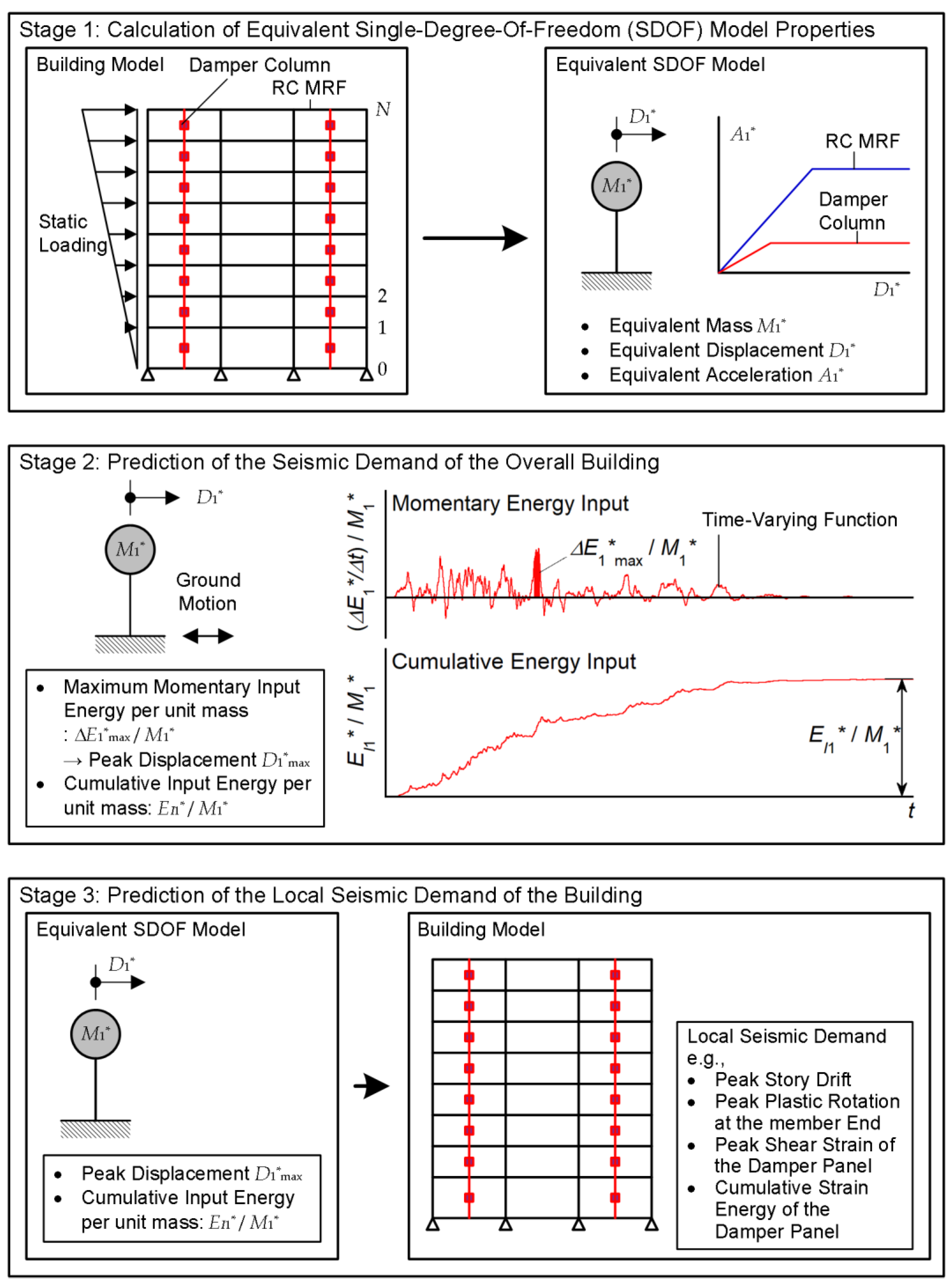
2.1. Stage 1: Calculation of the Equivalent SDOF Model Properties
2.1.1. Stage 1-1: Pushover Analysis of the Building Model
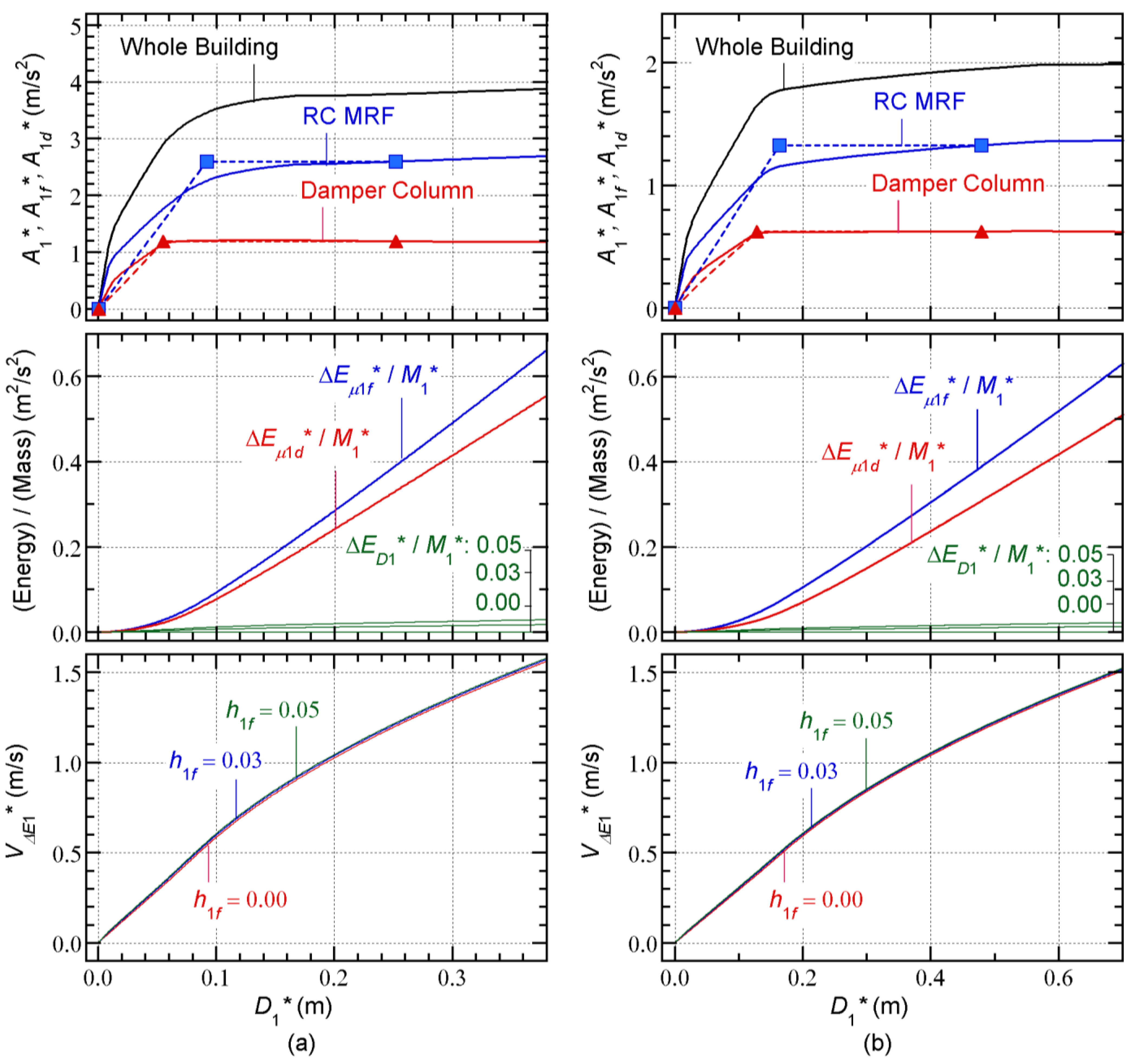
2.1.2. Stage 1-2: Calculation of the Capacity Curve of the Equivalent SDOF Model
2.2. Stage 2: Prediction of the Seismic Demand of the Overall Building
2.2.1. Stage 2-1: Calculation of V∆E and VI Spectra
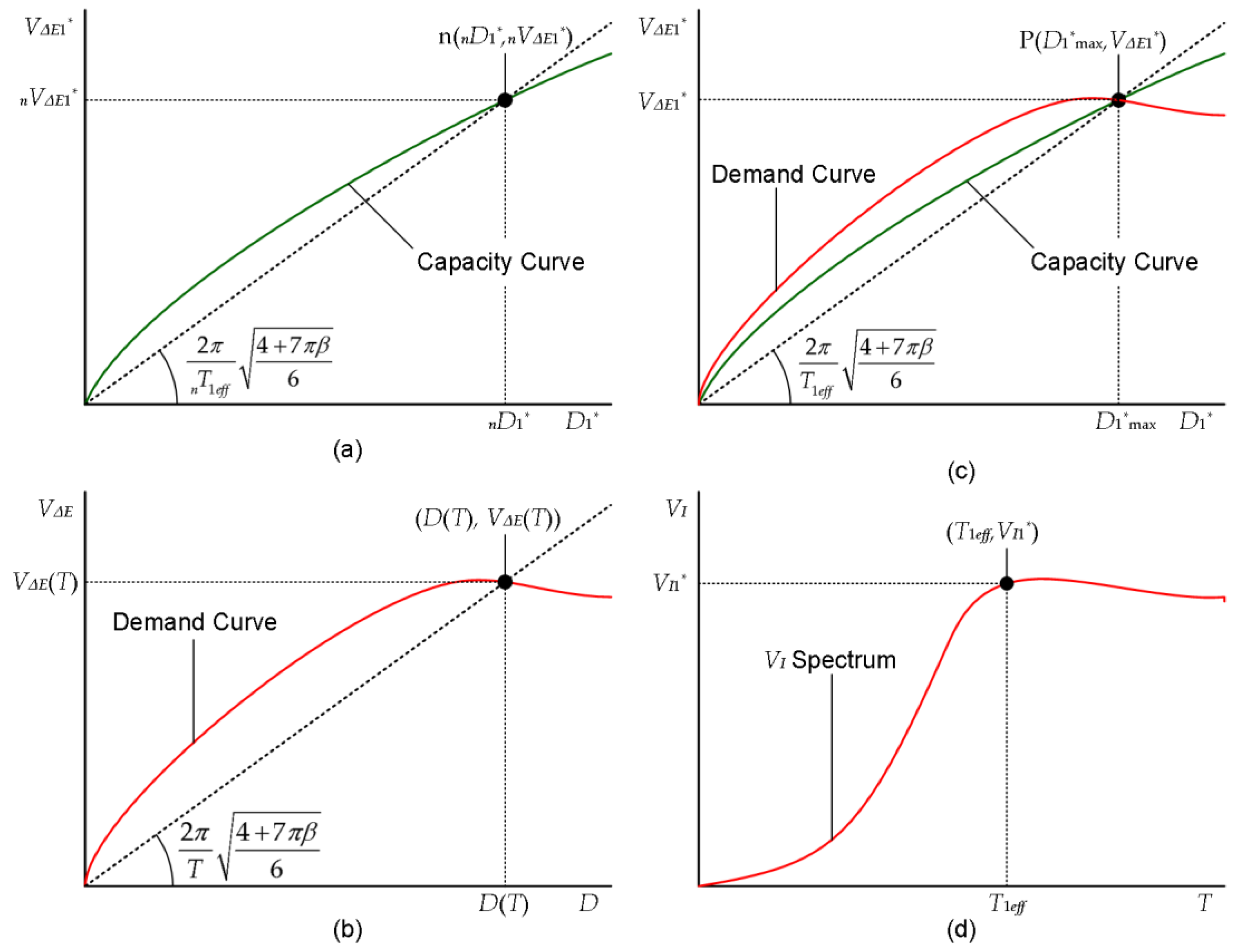
2.2.2. Stage 2-2: Calculation of Demand Curve
2.2.3. Stage 2-3: Determination of the Peak and Cumulative Response of the Equivalent SDOF Model
2.2.4. Stage 2-4: Calculation of the Cumulative Energies of the Overall Building
2.3. Stage 3: Prediction of the Local Seismic Demand of the Building Model
2.3.1. Stage 3-1: Determination of Peak Local Seismic Demand
2.3.2. Stage 3-2: Calculation of Cumulative Response Demand of Each Damper Column
3. Model Structures and Ground Motions
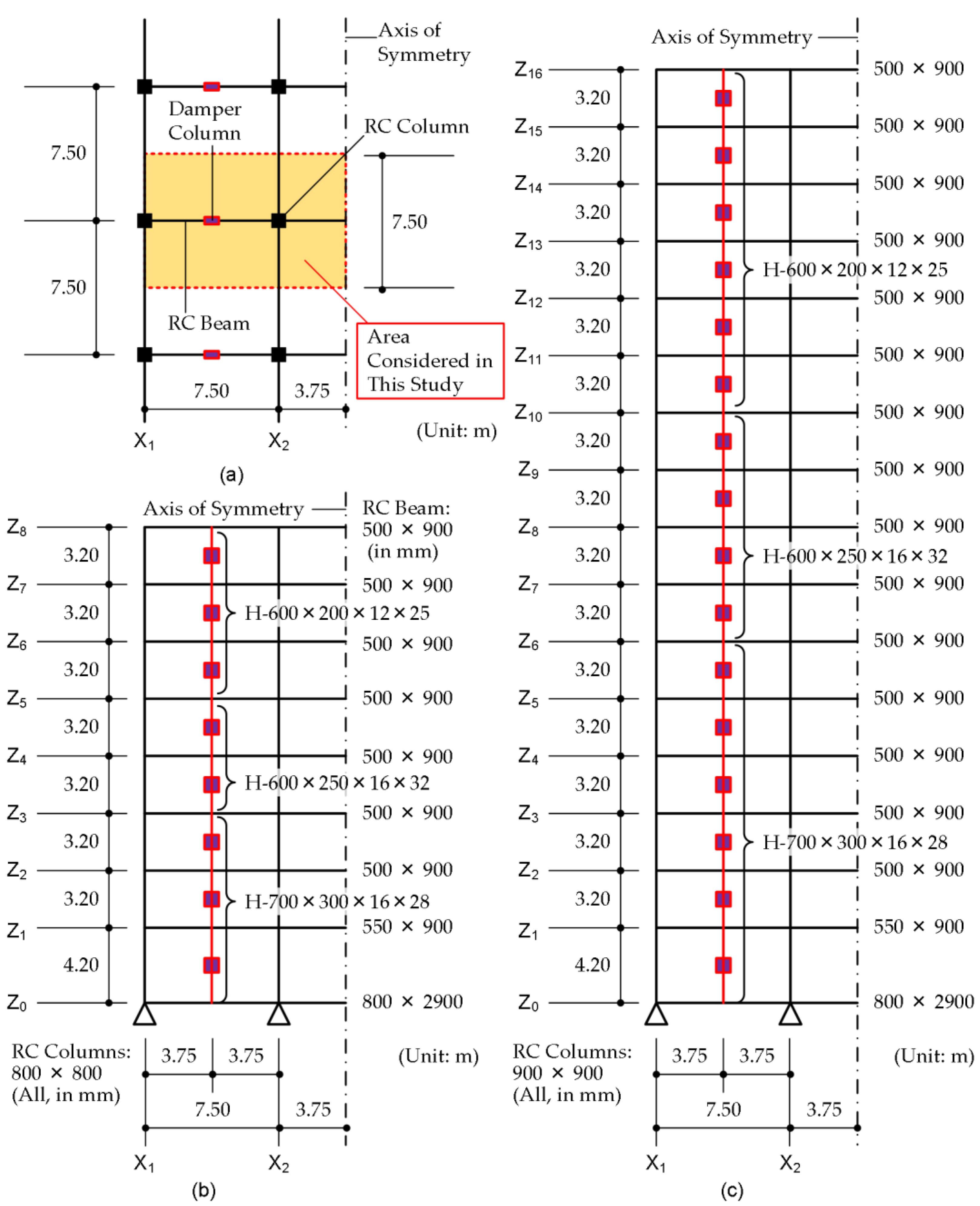
3.1. Model Structures
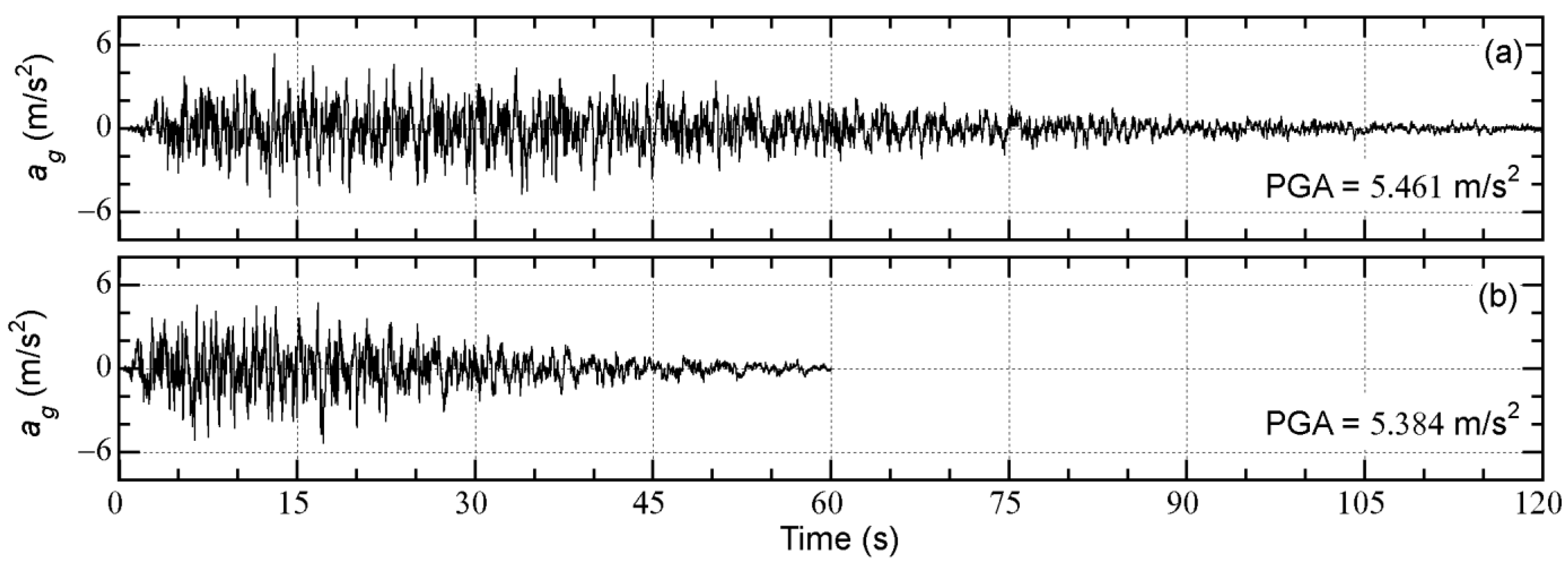
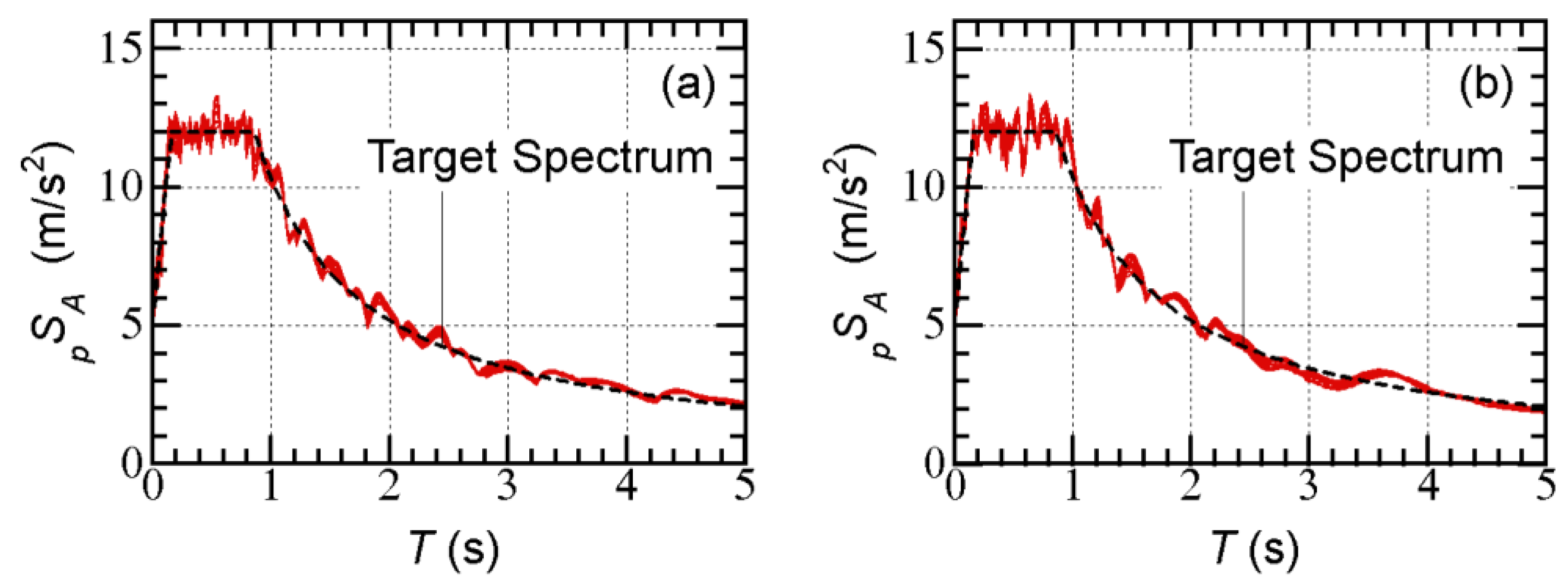
3.2. Ground Motions
3.3. Analysis Cases
- The complex damping ratio of the equivalent linear system (): the complex damping ratio of the equivalent linear system is the key parameter in obtaining better predictions of the energy response. Therefore, three different values of are considered: 0.05, 0.10, and 0.15.
- The viscous damping ratio of the first modal response of the RC MRFs in the elastic range (): the accuracy of the cumulative energy depends on the viscous damping of the RC MRFs. Therefore, three different values of are considered: 0.00, 0.03, and 0.05.
4. Analysis Results
4.1. Prediction of the Seismic Demand of the Equivalent SDOF Model
4.2. Comparisons with the Time-History Analysis Results
4.2.1. Energy Demand of the Overall Building
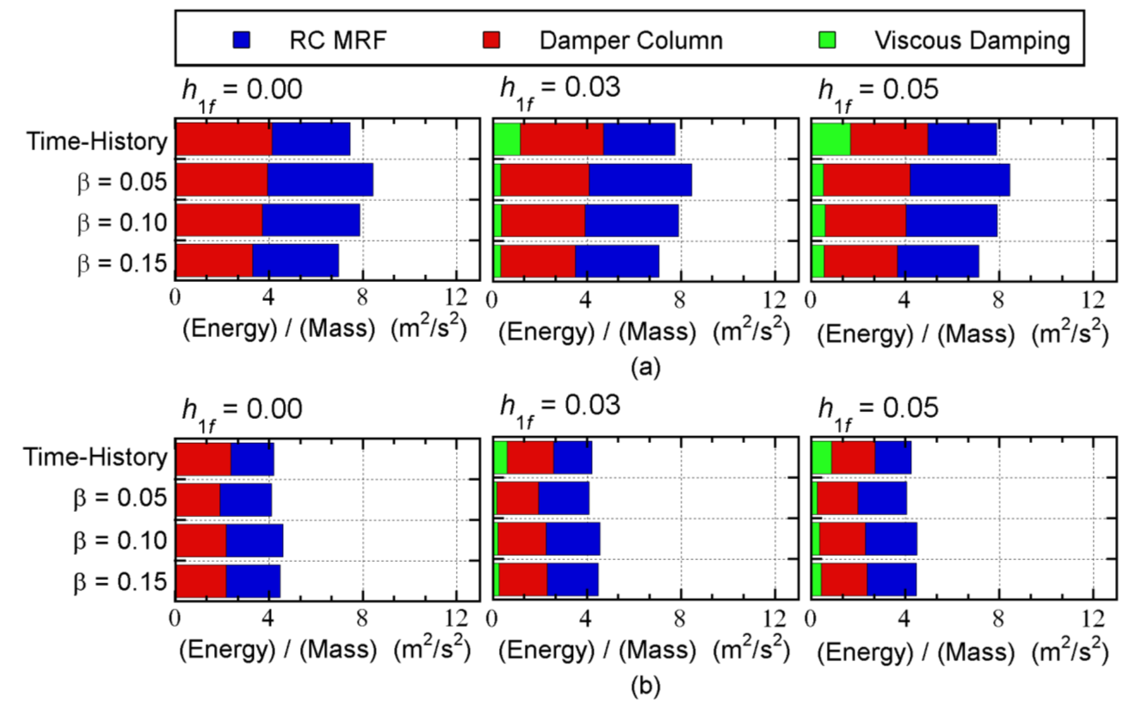
- For the 8-story model shown in Figure 10, the relationships between the predicted total input energies and the nonlinear time-history analysis results depend on the ground motion series and the value of : the predicted total input energy with = 0.15 is unconservative for all cases. For the 16-story building model shown in Figure 11, the predicted total input energy agrees well with that obtained from the nonlinear time-history analysis results for all cases.
- The predicted cumulative strain energy of the RC MRFs is larger than that obtained from the nonlinear time-history analysis results for both models.
- The predicted cumulative strain energy of the steel damper columns is close to that of the nonlinear time-history analysis results for both models.
- The predicted cumulative energy of viscous damping is smaller than that of the nonlinear time-history analysis results, except when = 0.00.
4.2.2. Local Seismic Demand
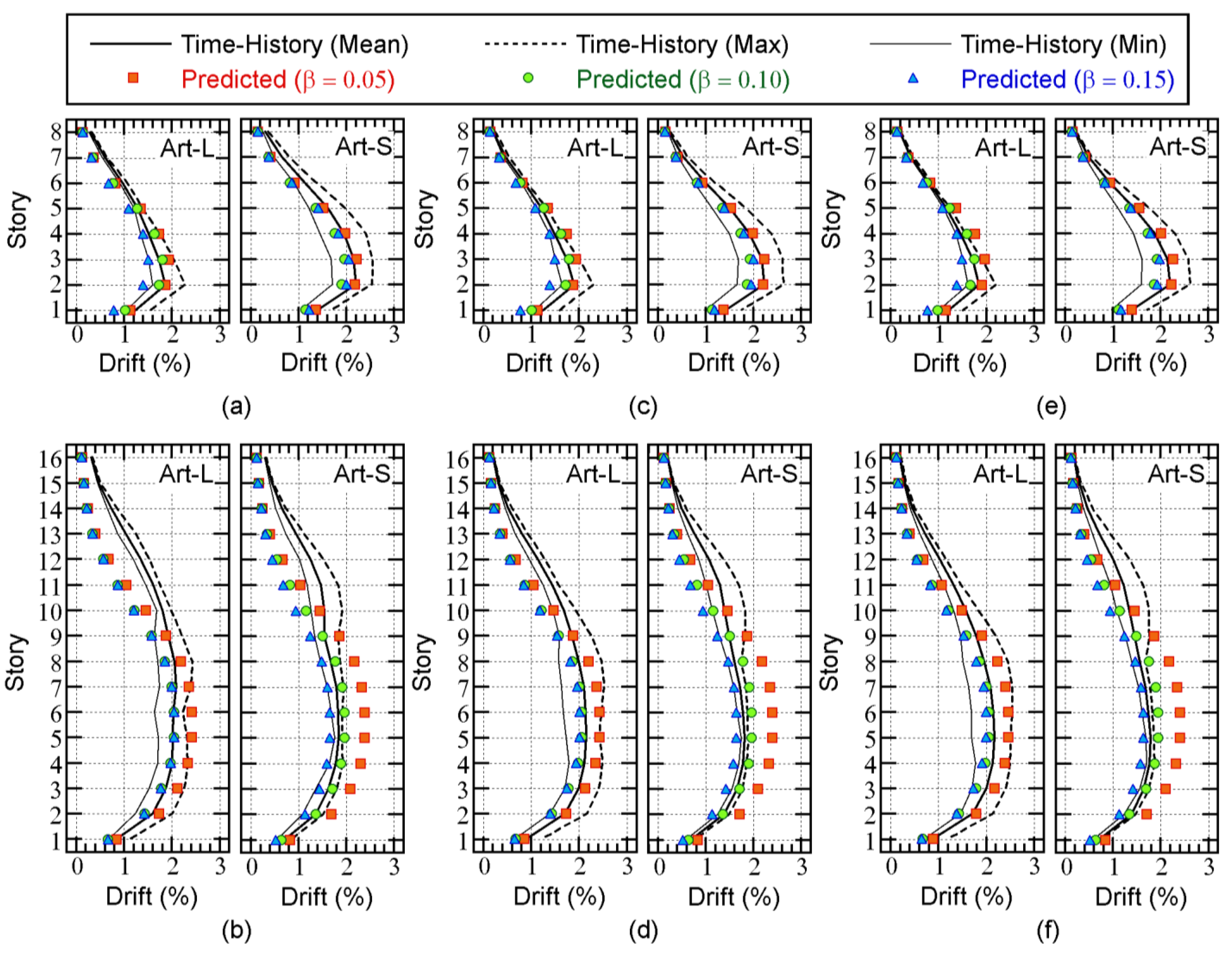
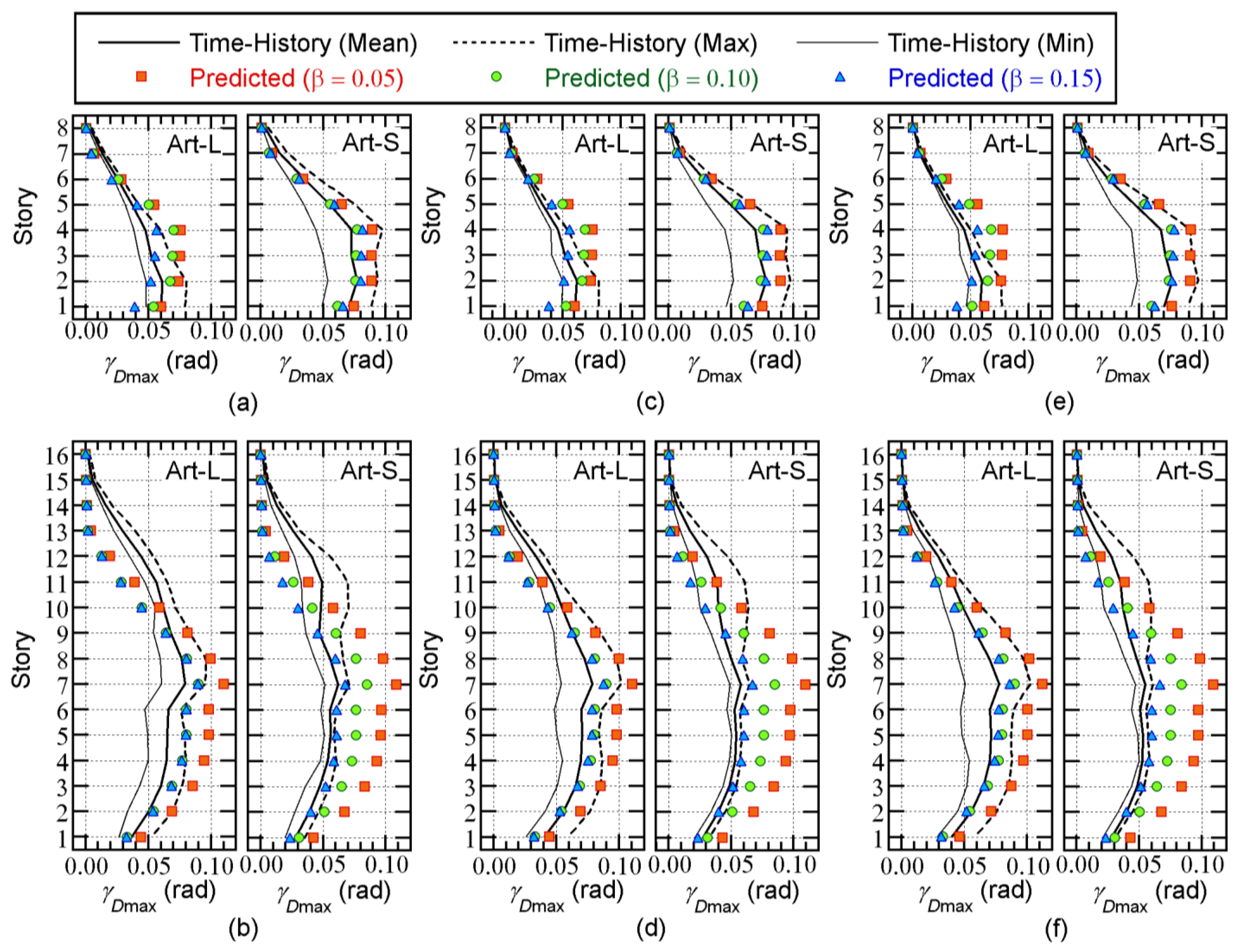
- For the 8-story model, the predicted peak drift with = 0.05 is larger than the mean of the nonlinear time-history analysis results, whereas the predicted peak drift with = 0.10 is slightly smaller than the mean of the nonlinear time-history analysis results. When = 0.15, the predicted peak drift is smaller than the mean of the nonlinear time-history analysis results.
- For the 16-story model, the predicted peak story drift with = 0.10 is in good agreement with the nonlinear time-history analysis results below the mid-story level (7th or 8th story). However, the predicted peak story drift above this level is lower than that of the nonlinear time-history analysis results. This tendency is noticeable when = 0.00.
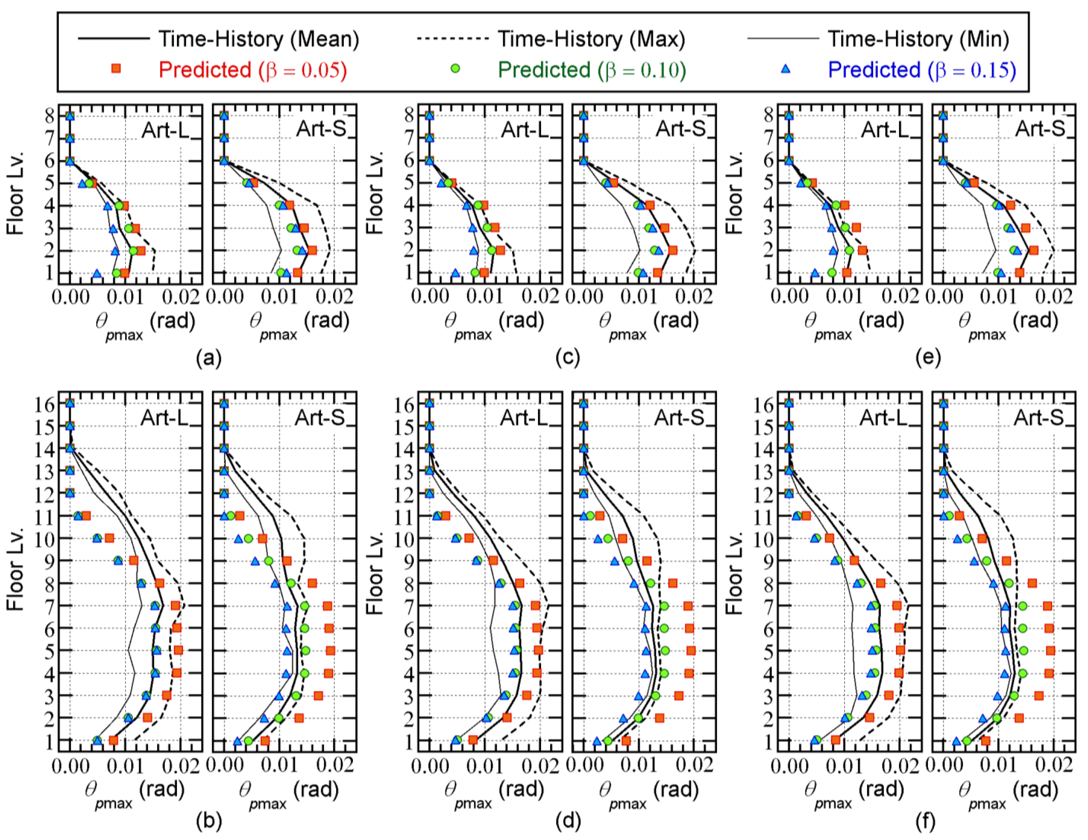
- For the 8-story model, the predicted with = 0.05 is slightly larger than the mean of the nonlinear time-history analysis results. The predicted are unconservative when = 0.10 or = 0.15.
- For the 16-story model, the predicted with = 0.05 is too conservative below the mid-story level (7th or 8th story). The predicted with = 0.10 agrees well with the mean of the nonlinear time-history analysis results below the mid-story level. For = 0.15, the predicted is unconservative for all floors.
- For the 8-story model, the predicted with = 0.05 is larger than the mean of the nonlinear time-history analysis results. The predicted for the cases where = 0.10 and = 0.15 are closer to the mean of the nonlinear time-history analysis results.
- For the 16-story model, the predicted with = 0.05 is too conservative below the mid-story level (9th or 10th story). The predicted when = 0.10 is also conservative below the mid-story level, but is closer to the mean of the nonlinear time-history analysis results. The predicted with = 0.15 is the closest to the mean of the nonlinear time-history analysis results.
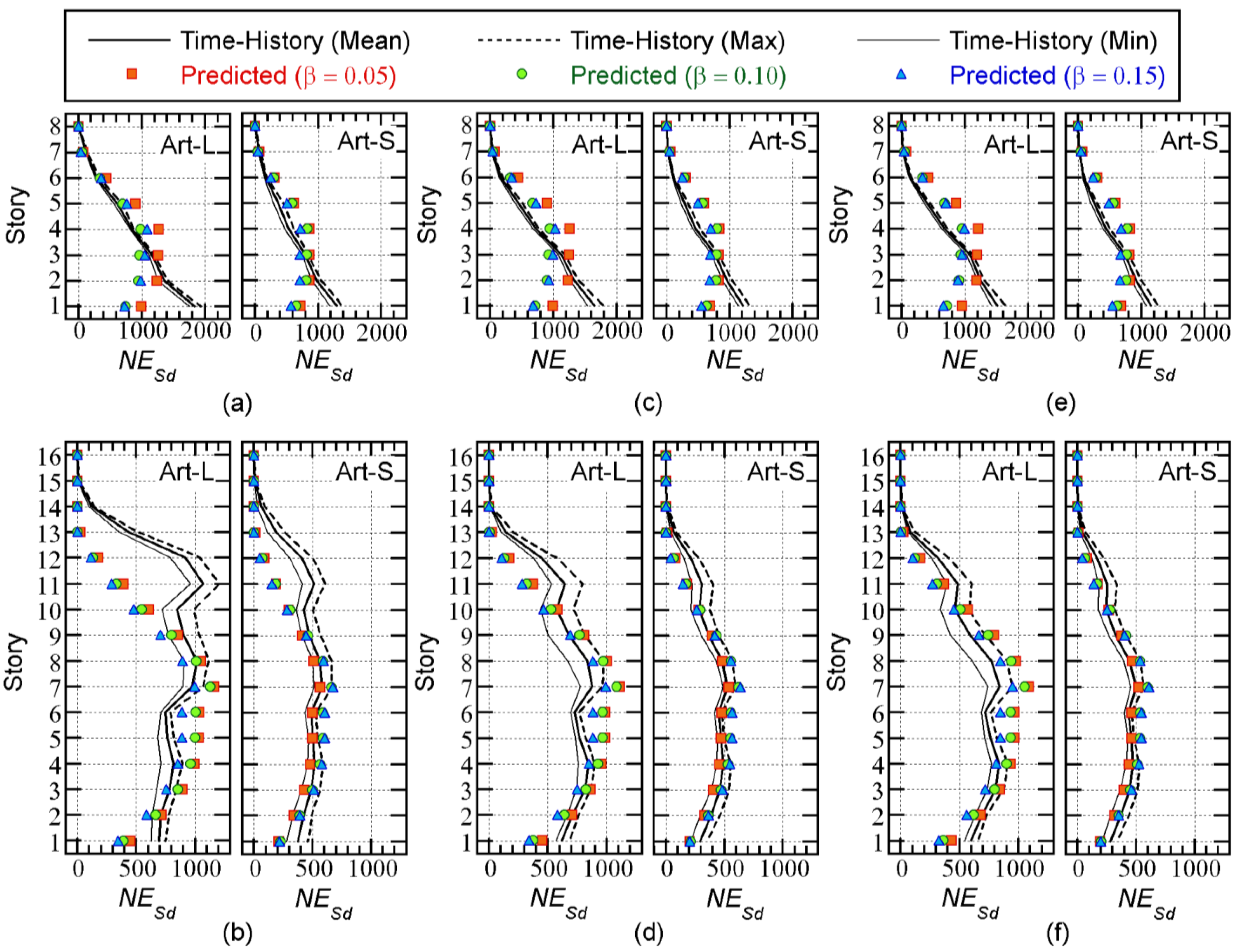
- For the 8-story model, the predicted is larger than that of the nonlinear time-history analysis results above the second story. However, the predicted at the first story underestimates the nonlinear time-history analysis results.
- For the 16-story building model, the predicted is in good agreement with the nonlinear analysis results below the mid-story level (9th or 10th story). However, the predicted above the mid-story level underestimates the nonlinear time-history analysis results. This is noticeable when = 0.00.
4.3. Summary of the Analysis Results
- The accuracy of the predicted energy demand of the whole building is acceptable, although the predicted cumulative energy of viscous damping is small.
- The accuracy of the predicted local peak seismic demands (story drift, plastic rotation of the beam end, and shear strain of the damper panels) is acceptable, although some quantities are unconservative.
- The accuracy of the predicted cumulative energy strain energy demand of the damper panels is acceptable, although some values are unconservative.
5. Discussion
5.1. Applicability of the Time-Varying Function of the Momentary Energy Input for Predicting the Energy Response
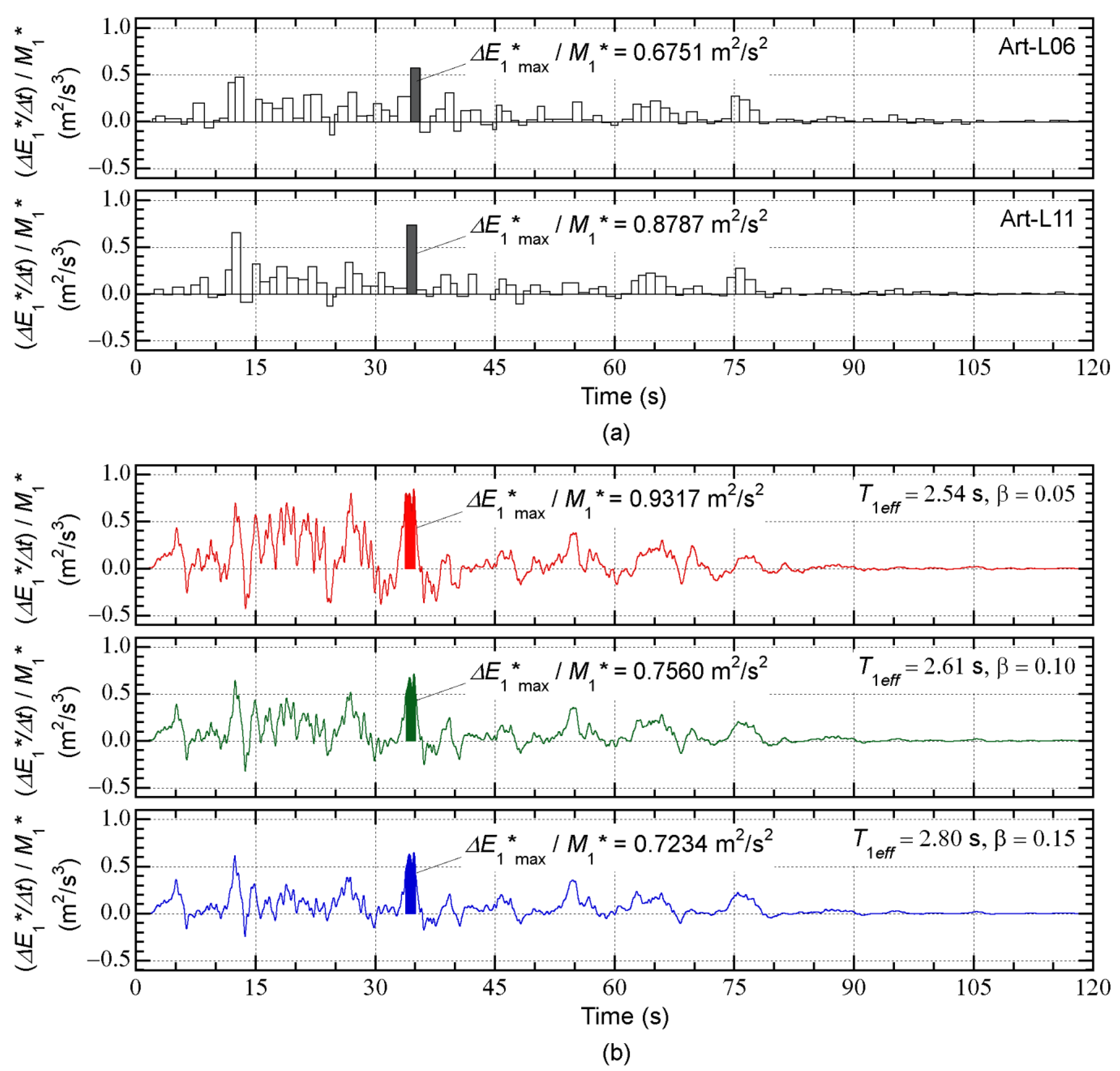
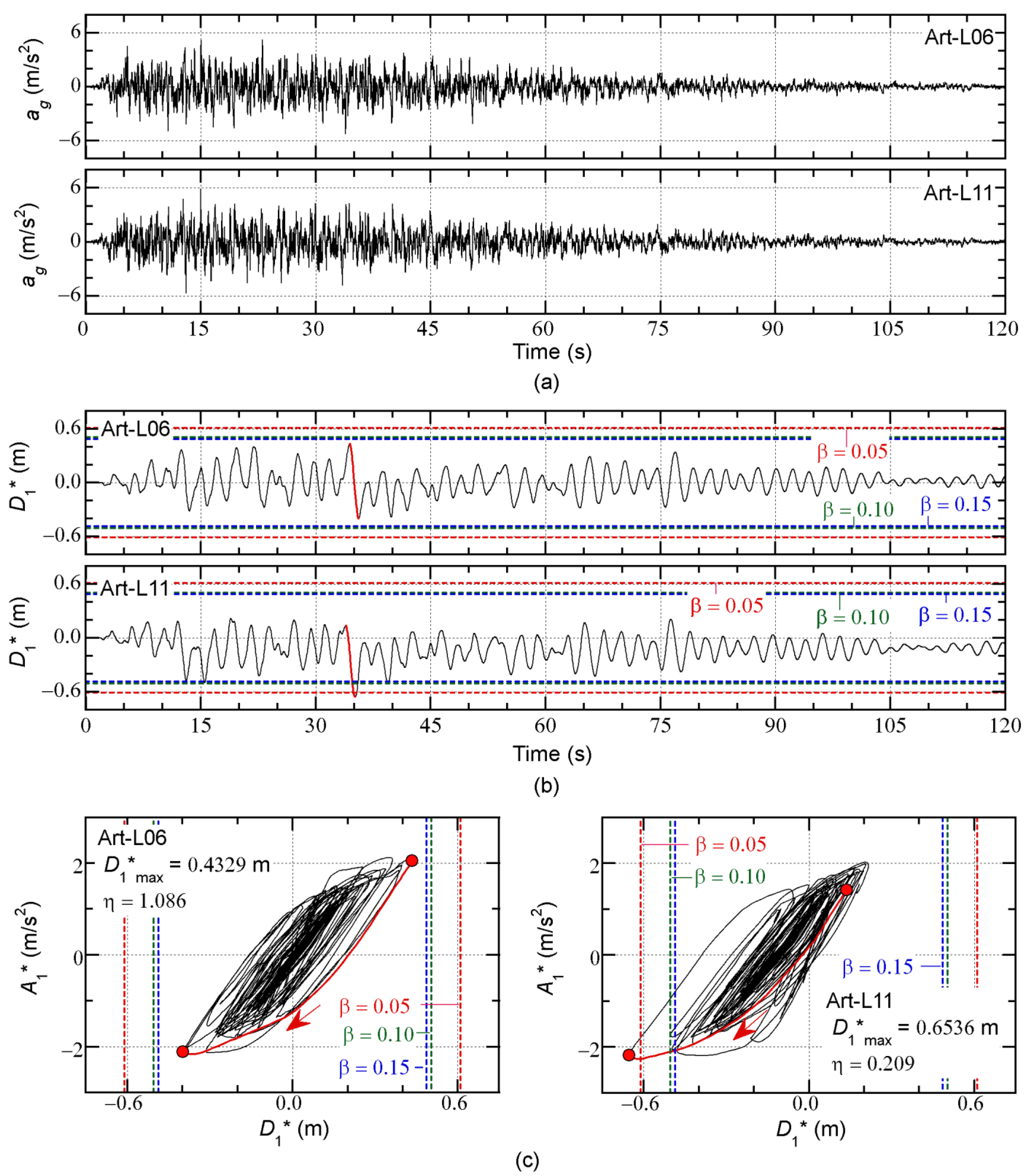
- Although the time-histories of the ground accelerations are very similar, the time-histories of the equivalent displacement are different. The equivalent displacement does not exceed the predicted in the case of Art-L-06, but does exceed the predicted in the case of Art-L-11.
- The time-histories of the momentary input energy are very similar for Art-L-06 and Art-L-11, although is different, being larger for Art-L-11 than for Art-L-06.
- The time-varying functions calculated assuming = 0.05 (shown at the top of Figure 17b) are notably different from the nonlinear time-history analysis results shown in Figure 17a: the variations in the time-varying functions are too large in comparison with the nonlinear time-history analysis results.
- The time-varying functions calculated assuming = 0.10 and 0.15 (shown in the middle and bottom of Figure 17b) are closer to the nonlinear time-history analysis results than those for = 0.05. In addition, the value of calculated from the time-varying function is between the values for Art-L-06 and Art-L-11. The calculated for = 0.10 is larger than that for = 0.15.
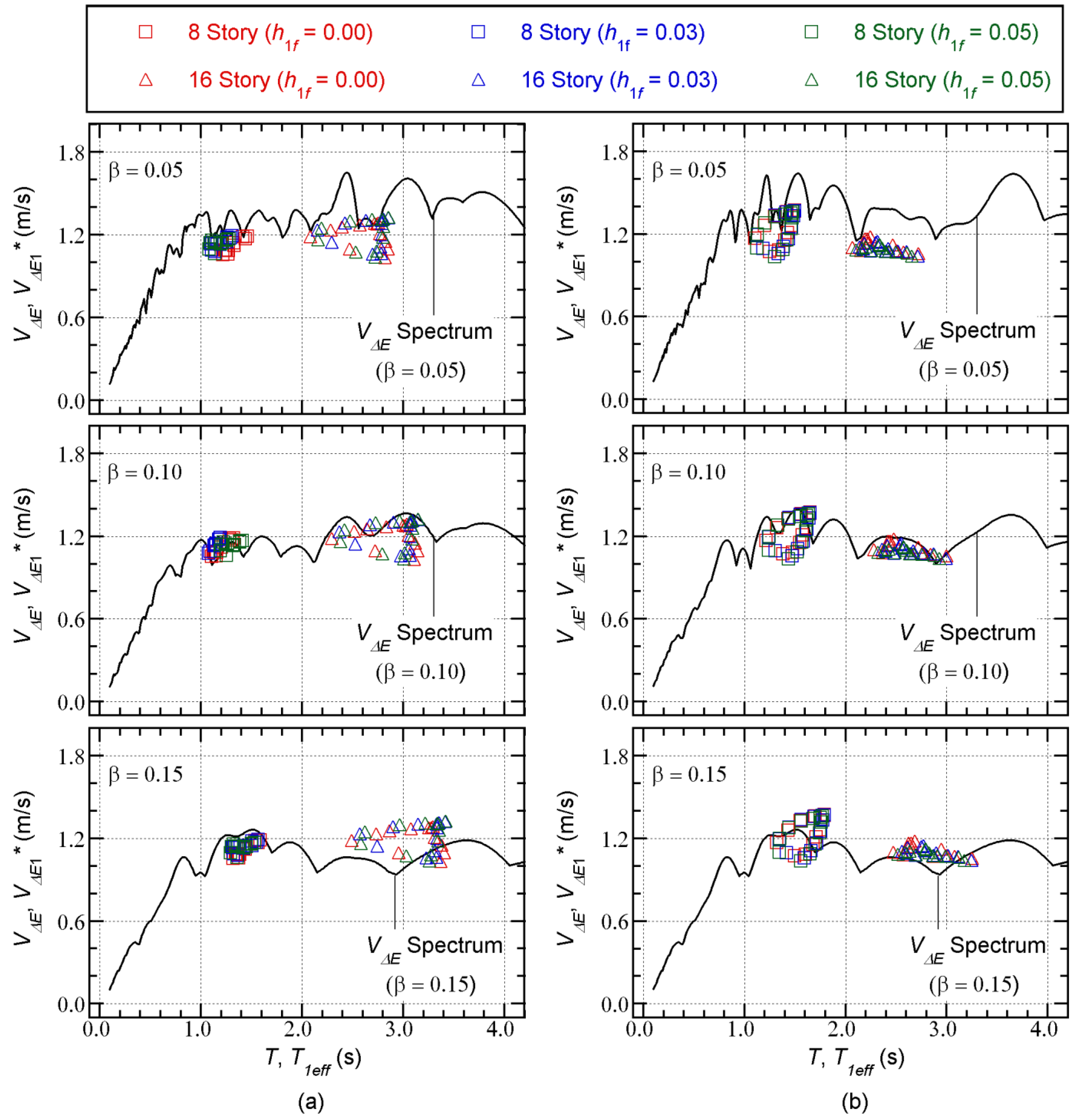
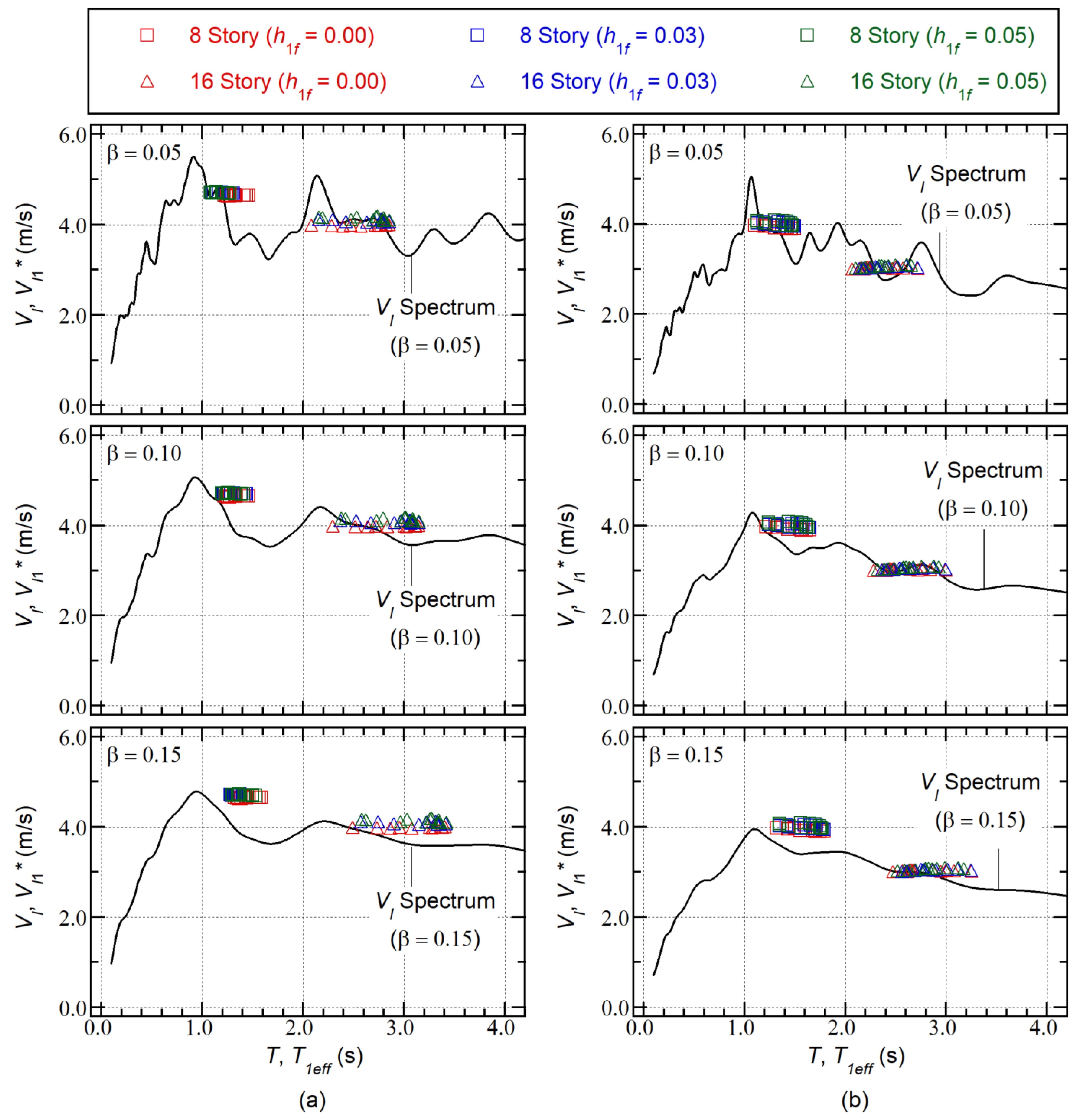
- In the case of = 0.05 (shown at the top of Figure 18), the nonlinear time-history analysis results are below the spectrum.
- In the case of = 0.10 (shown in the middle of Figure 18), the nonlinear time-history analysis results are in good agreement with the spectrum.
- In the case of = 0.15 (shown at the bottom of Figure 18), some of the nonlinear time-history analysis results are above the spectrum.
5.2. Relationship between Maximum Momentary Input Energy of the First Modal Response and the Peak Equivalent Displacement
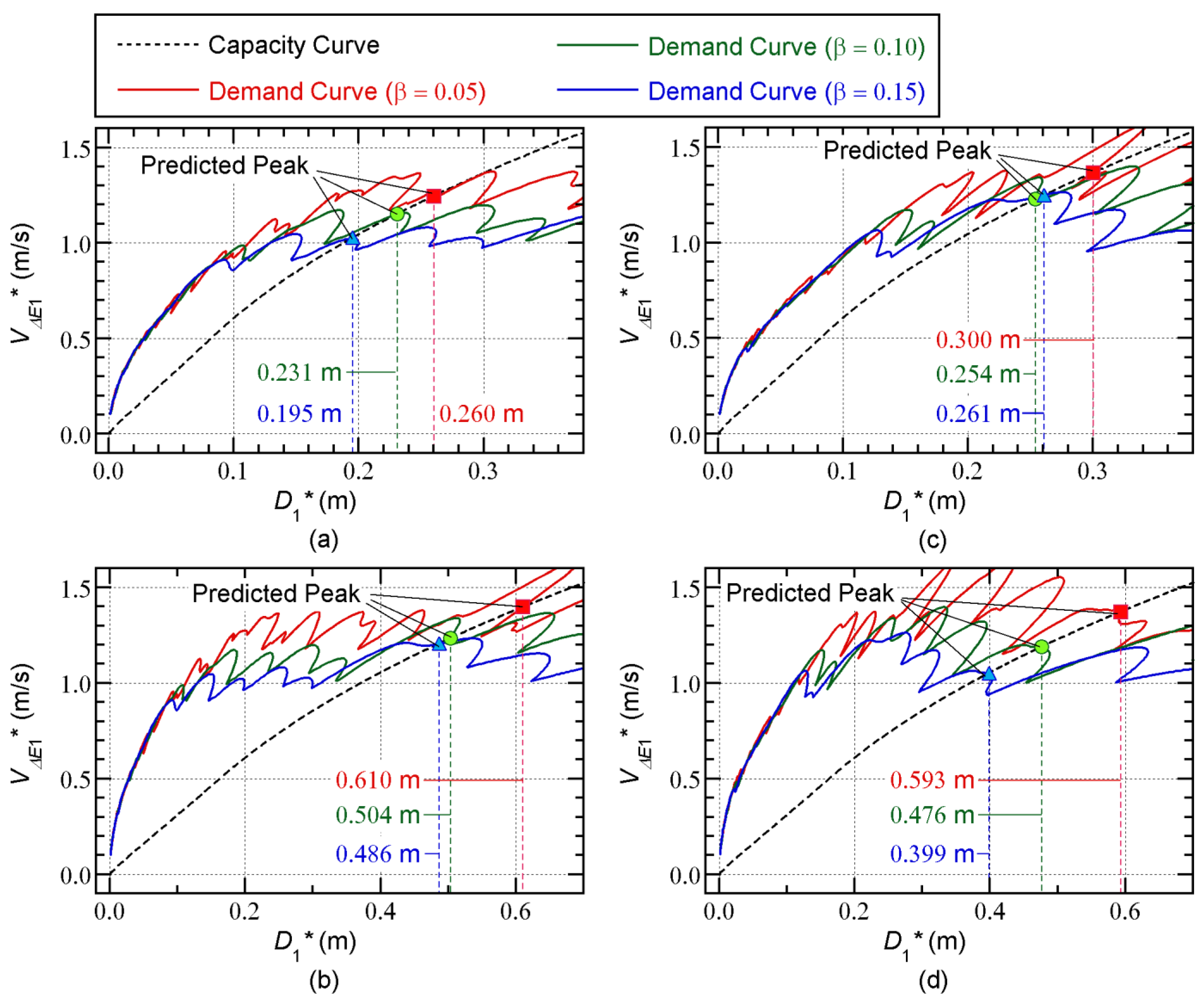
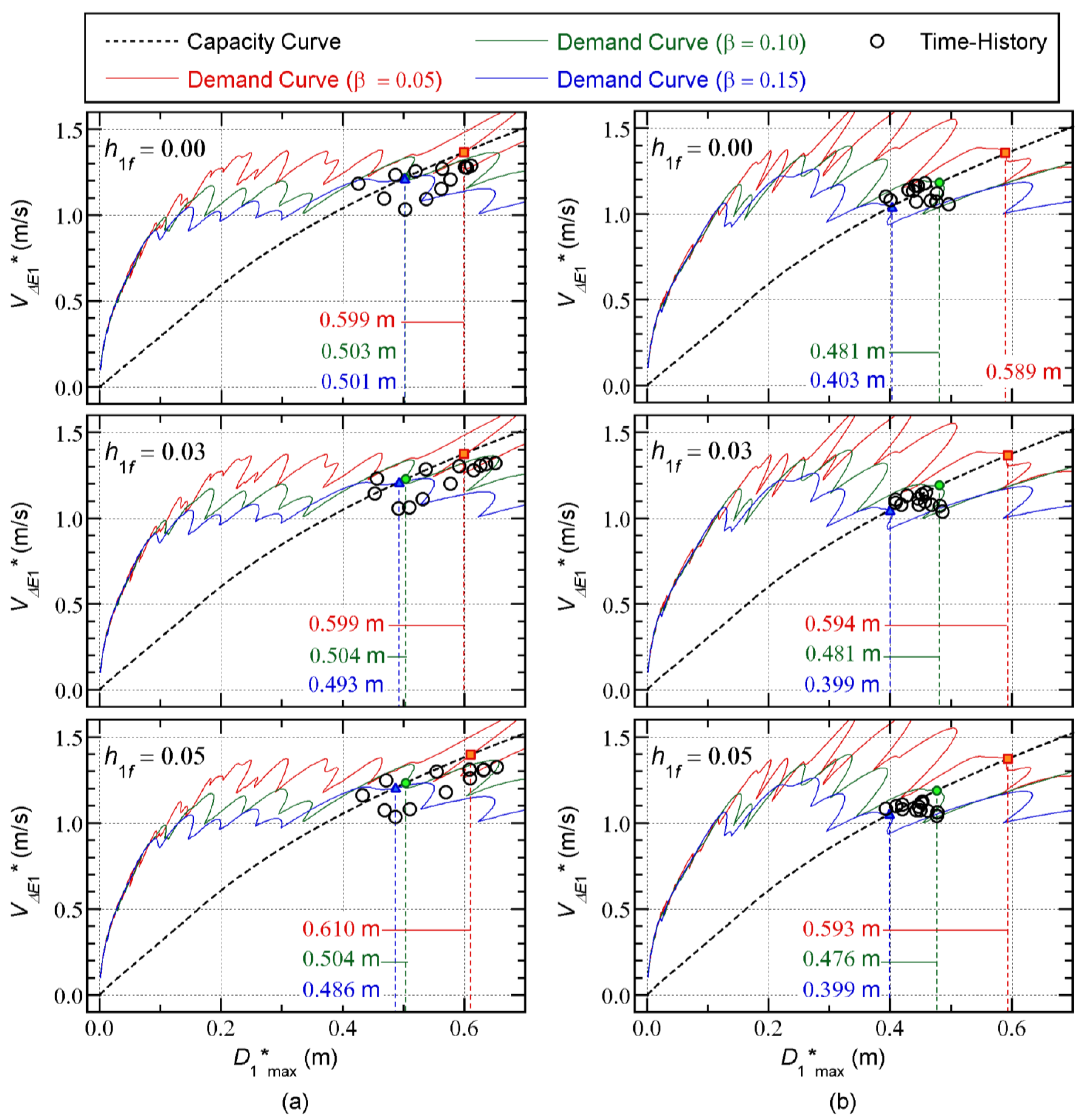
- Most of the nonlinear history analysis results are slightly below the capacity curve. The scatter of the nonlinear time-history analysis results is noticeable in the case of the Art-S series for the 8-story model and the Art-L series for the 16-story model.
- In most cases, the predicted peak response point with = 0.05 gives the most conservative . The predicted with = 0.10 is slightly unconservative, and the predicted with = 0.15 is unconservative.
5.3. Summary of Discussions
- The equivalent velocities of the maximum momentary input energy and the cumulative energy ( and ) can be properly predicted using the time-varying function, an appropriate effective period , and = 0.10. For the calculation of , Equation (33) is suitable.
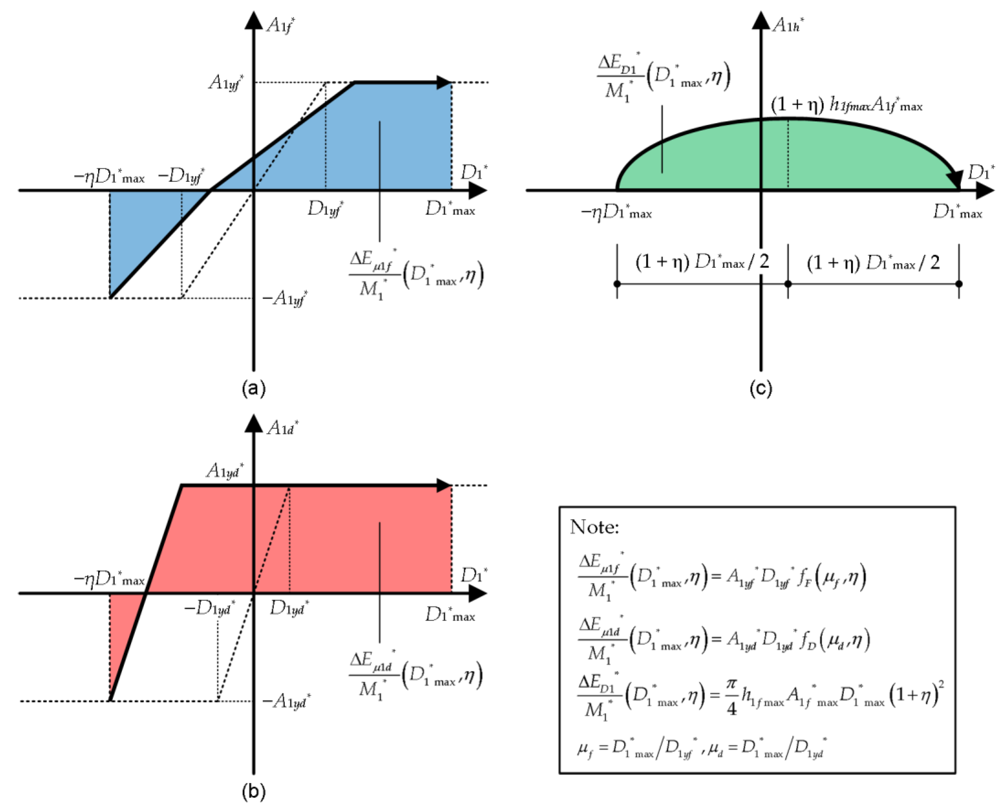
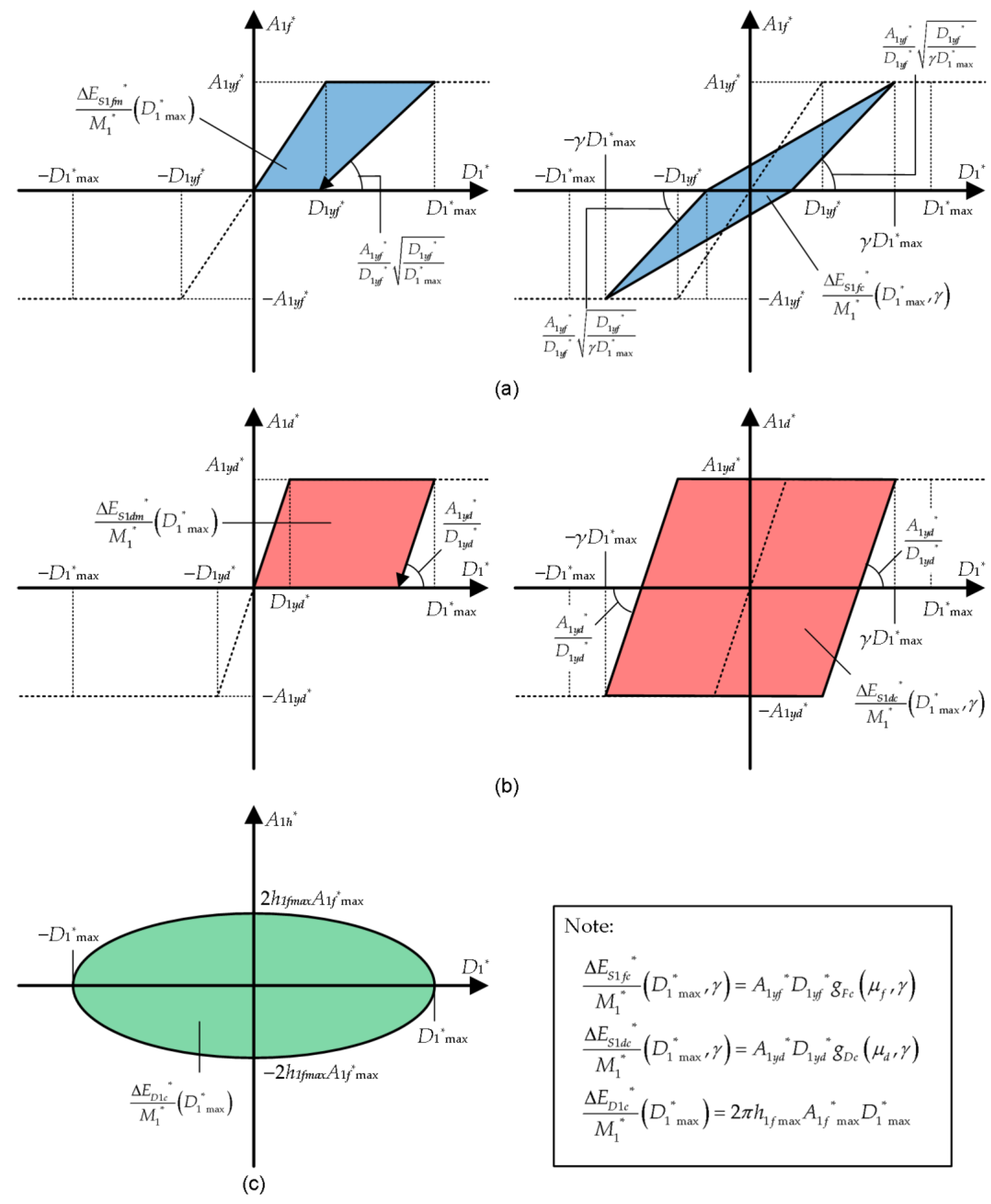
- For better predictions of the peak response, the capacity curve should be properly calculated. It is also very important to evaluate the dissipated energy during a half cycle of the structural response, in addition to better predicting the maximum momentary input energy.
6. Conclusions
- The time-varying function of the momentary energy input provides sufficiently accurate predictions of the maximum momentary input energy and the cumulative input energy of RC MRFs with steel damper columns. The time-history of the momentary input energy calculated using the time-varying function is close to the nonlinear time-history analysis results. An equation for calculating the effective period of the first modal response from the peak equivalent displacement and the equivalent velocity of the maximum momentary input energy has been developed. Based on the cases considered in this study, the recommended value of the complex damping ratio is 0.10.
- The accuracy of the predicted local peak seismic demand (e.g., story drift, plastic rotation of the beam end, and shear strain of the damper panel) is acceptable, although some values are unconservative.
- The accuracy of the predicted cumulative energy strain energy demand of the damper panel is acceptable, although some values are unconservative.
- For better predictions of the peak response, the capacity curve must be properly calculated. It is also very important to evaluate the energy dissipated during a half cycle of the structural response, and to obtain better predictions of the maximum momentary input energy.
- The ground motions used in this study are non-pulsive artificial ground accelerations. In the case of RC MRFs with damper columns subjected to near-fault pulsive ground motions, how accurate is the proposed procedure? Does it offer the same performance as in this study?
- In this study, the cumulative strain energy was only evaluated for the damper columns. The influence of cyclic loading on the damage to RC members may not be significant in the case of ductile RC members within a certain drift limit (e.g., less than 0.02 radians [42]). However, in the case of RC members with larger drift demands, the cumulative strain energy demand would be needed. How can the cumulative strain energy of the RC members be evaluated in a simple manner?
- Several studies on the applicability of pushover analysis to planar frames [33,34,35,36,37,38,39,40] have shown that the contribution of higher modes is notable in the case of mid- to high-rise buildings. We believe that, according to the peak response, the proposed procedure can be applied in such cases without difficultly. However, there is room for discussion in terms of predicting the cumulative response of each member. How can the contribution of higher modal responses be considered for the prediction of the local cumulative response?
- In the hysteresis of RC members, pinching behavior [41] is observed in cyclic loading tests. This behavior may affect the hysteretic energy dissipation of RC MRFs with damper columns. Specifically, the pinching behavior of the RC beams surrounding damper columns may reduce the energy absorption of the damper panel. Is this a negligible effect in predicting the seismic demand of ductile RC MRFs with damper columns? If not, how can the influence of pinching behavior be considered in modeling the hysteretic energy dissipation in a half cycle of the structural response?
- The response of RC MRFs with damper columns subjected to sequential ground motions has previously been investigated [7]. It is expected that the proposed procedure may be applicable to such sequential ground motions if the influence of prior damage to each member can be included when calculating the dissipated hysteretic energy during a half cycle of the structural response. How can models for the calculation of dissipated energies be extended to the case of sequential ground motions?
Author Contributions
Funding
Institutional Review Board Statement
Informed Consent Statement
Data Availability Statement
Acknowledgments
Conflicts of Interest
Appendix A. Formulation of the Dissipated Energy in a Half Cycle
Appendix B. Formulation of the Effective Period

Appendix C. Formulation of the Cumulative Dissipated Energy

Appendix D. Model Properties

| Member | Location | Width (mm) | Depth (mm) | Longitudinal Reinforcement |
|---|---|---|---|---|
| Z4 to Z8 | 500 | 900 | 5-D29 (Top and bottom) | |
| Beam | Z2 to Z3 | 500 | 900 | 5-D32 (Top and bottom) |
| Z1 | 550 | 900 | 5-D35 (Top and bottom) | |
| Column | 1st Story (Bottom) | 800 | 800 | 16-D29 (Total) |
| Story | Yield Strength | Panel Thickness (mm) | Panel Height (mm) | Panel Sectional Area (mm2) | Column (mm × mm × mm × mm) | |
|---|---|---|---|---|---|---|
| QyDL (kN) | QyDU (kN) | |||||
| 6 to 8 | 438 | 641 | 6 | 600 | 3700 | H-600 × 200 × 12 × 25 |
| 4 to 5 | 626 | 916 | 9 | 600 | 5290 | H-600 × 250 × 16 × 32 |
| 1 to 3 | 755 | 1105 | 9 | 700 | 6380 | H-700 × 300 × 16 × 28 |
| Member | Location | Width (mm) | Depth (mm) | Longitudinal Reinforcement |
|---|---|---|---|---|
| Z7 to Z16 | 500 | 900 | 5-D29 (Top and bottom) | |
| Beam | Z2 to Z6 | 500 | 900 | 5-D32 (Top and bottom) |
| Z1 | 550 | 900 | 5-D35 (Top and bottom) | |
| Column | 1st Story (Bottom) | 900 | 900 | 16-D32 (Total) |
| Story | Yield Strength | Panel Thickness (mm) | Panel Height (mm) | Panel Sectional Area (mm2) | Column (mm × mm × mm × mm) | |
|---|---|---|---|---|---|---|
| QyDL (kN) | QyDU (kN) | |||||
| 11 to 16 | 438 | 641 | 6 | 600 | 3700 | H-600 × 200 × 12 × 25 |
| 7 to 10 | 626 | 916 | 9 | 600 | 5290 | H-600 × 250 × 16 × 32 |
| 1 to 6 | 755 | 1105 | 9 | 700 | 6380 | H-700 × 300 × 16 × 28 |
References
- Wada, A.; Huang, Y.H.; Iwata, M. Passive damping technology for building in Japan. Prog. Struct. Eng. Mater. 2000, 8, 335–350. [Google Scholar] [CrossRef]
- Katayama, T.; Ito, S.; Kamura, H.; Ueki, T.; Okamoto, H. Experimental study on hysteretic damper with low yield strength steel under dynamic loading. In Proceedings of the 12th World Conference on Earthquake Engineering, Auckland, New Zealand, 30 January–4 February 2000. [Google Scholar]
- Fujii, K.; Miyagawa, K. Nonlinear seismic response of a seven-story steel reinforced concrete condominium retrofitted with low-yield-strength-steel damper columns. In Proceedings of the 16th European Conference on Earthquake Engineering, Thessaloniki, Greece, 18–21 June 2018. [Google Scholar]
- Fujii, K.; Sugiyama, H.; Miyagawa, K. Predicting the peak seismic response of a retrofitted nine-story steel reinforced concrete building with steel damper columns. WIT Trans. Built Environ. 2019, 185, 75–85. [Google Scholar] [CrossRef]
- Mukouyama, R.; Fujii, K.; Irie, C.; Tobari, R.; Yoshinaga, M.; Miyagawa, K. Displacement-controlled seismic design method of reinforced concrete frame with steel damper column. In Proceedings of the 17th World Conference on Earthquake Engineering, Sendai, Japan, 27 September–2 October 2021. [Google Scholar]
- Fujii, K.; Kato, M. Strength balance of steel damper columns and surrounding beams in reinforced concrete frames. WIT Trans. Built Environ. 2021, 202, 25–36. [Google Scholar] [CrossRef]
- Fujii, K. Peak and Cumulative Response of Reinforced Concrete Frames with Steel Damper Columns under Seismic Sequences. Buildings 2022, 12, 275. [Google Scholar] [CrossRef]
- Park, Y.J.; Ang, A.H.S. Mechanistic seismic damage model for reinforced concrete. J. Struct. Eng. ASCE 1985, 111, 722–739. [Google Scholar] [CrossRef]
- Architectural Institute of Japan (AIJ). Recommended Provisions for Seismic Damping Systems Applied to Steel Structures; Architectural Institute of Japan: Tokyo, Japan, 2014. (In Japanese) [Google Scholar]
- Akiyama, H. Earthquake–Resistant Limit–State Design for Buildings; University of Tokyo Press: Tokyo, Japan, 1985. [Google Scholar]
- Uang, C.M.; Bertero, V.V. Evaluation of seismic energy in structures. Earthq. Eng. Struct. Dyn. 1990, 19, 77–90. [Google Scholar] [CrossRef]
- Fajfar, P.; Vidic, T. Consistent inelastic design spectra: Hysteretic and input energy. Earthq. Eng. Struct. Dyn. 1994, 23, 523–537. [Google Scholar] [CrossRef]
- Sucuoǧlu, H.; Nurtuǧ, A. Earthquake ground motion characteristics and seismic energy dissipation. Earthq. Eng. Struct. Dyn. 1995, 24, 1195–1213. [Google Scholar] [CrossRef]
- Nurtuǧ, A.; Sucuoǧlu, H. Prediction of seismic energy dissipation in SDOF systems. Earthq. Eng. Struct. Dyn. 1995, 24, 1215–1223. [Google Scholar] [CrossRef]
- Chai, Y.H.; Fajfar, P.; Romstad, K.M. Formulation of duration-dependent inelastic seismic design spectrum. J. Struct. Eng. 1998, 124, 913–921. [Google Scholar] [CrossRef]
- Cheng, Y.; Lucchini, A.; Mollaioli, F. Ground-motion prediction equations for constant-strength and constant-ductility input energy spectra. Bull. Earthq. Eng. 2020, 18, 37–55. [Google Scholar] [CrossRef]
- Fajfar, P.; Gaspersic, P. The N2 method for the seismic damage analysis of RC buildings. Earthq. Eng. Struct. Dyn. 1996, 25, 31–46. [Google Scholar] [CrossRef]
- Ghosh, S.; Datta, D.; Katakdhond A., A. Estimation of the Park–Ang damage index for planar multi-storey frames using equivalent single-degree systems. Eng. Struct. 2011, 33, 2509–2524. [Google Scholar] [CrossRef]
- Diaz, S.A.; Pujades, L.G.; Barbat, A.H.; Vargas, Y.F.; Hidalgo-Leiva, D.A. Energy damage index based on capacity and response spectra. Eng. Struct. 2017, 152, 424–436. [Google Scholar] [CrossRef]
- Fajfar, P. Equivalent ductility factors, taking into account low-cycle fatigue. Earthq. Eng. Struct. Dyn. 1992, 21, 837–848. [Google Scholar] [CrossRef]
- D’Ambrisi, A.; Mezzi, M. An energy-based approach for nonlinear static analysis of structures. Bull. Earthq. Eng. 2015, 13, 1513–1530. [Google Scholar] [CrossRef]
- Ucar, T. Computing input energy response of MDOF systems to actual ground motions based on modal contributions. Earthq. Struct. 2020, 18, 263–273. [Google Scholar]
- Yalçın, C.; Dindar, A.A.; Yüksel, E.; Özkaynak, H.; Büyüköztürk, O. Seismic design of RC frame structures based on energy-balance method. Eng. Struct. 2021, 237, 112220. [Google Scholar] [CrossRef]
- Benavent-Climent, A.; Mollaioli, F. (Eds.) Energy-Based Seismic Engineering; Springer Nature: Cham, Switzerland, 2021. [Google Scholar]
- Nakamura, T.; Hori, N.; Inoue, N. Evaluation of damaging properties of ground motions and estimation of maximum displacement based on momentary input energy. J. Struct. Constr. Eng. Trans. AIJ 1998, 63, 65–72. (In Japanese) [Google Scholar] [CrossRef]
- Inoue, N.; Wenliuhan, H.; Kanno, H.; Hori, N.; Ogawa, J. Shaking Table Tests of Reinforced Concrete Columns Subjected to Simulated Input Motions with Different Time Durations. In Proceedings of the 12th World Conference on Earthquake Engineering, Auckland, New Zealand, 30 January–4 February 2000. [Google Scholar]
- Hori, N.; Inoue, N. Damaging properties of ground motion and prediction of maximum response of structures based on momentary energy input. Earthq. Eng. Struct. Dyn. 2002, 31, 1657–1679. [Google Scholar] [CrossRef]
- Fujii, K.; Kanno, H.; Nishida, T. Formulation of the time-varying function of momentary energy input to a SDOF system by Fourier series. J. Jpn. Assoc. Earthq. Eng. 2019, 19, 247–266. [Google Scholar] [CrossRef]
- Fujii, K.; Murakami, Y. Bidirectional momentary energy input to a one-mass two-DOF system. In Proceedings of the 17th World Conference on Earthquake Engineering, Sendai, Japan, 20 September–2 November 2021. [Google Scholar]
- Fujii, K. Bidirectional seismic energy input to an isotropic nonlinear one-mass two-degree-of-freedom system. Buildings 2021, 11, 143. [Google Scholar] [CrossRef]
- Fujii, K.; Masuda, T. Application of Mode-Adaptive Bidirectional Pushover Analysis to an Irregular Reinforced Concrete Building Retrofitted via Base Isolation. Appl. Sci. 2021, 11, 9829. [Google Scholar] [CrossRef]
- Fajfar, P.; Fischinger, M. N2-A method for non-linear seismic analysis of regular buildings. In Proceedings of the 9th World Conference on Earthquake Engineering , Tokyo-Kyoto, Japan, 2–9 August 1988. [Google Scholar]
- Chopra, A.K.; Goel, R.K. A modal pushover analysis procedure for estimating seismic demands for buildings. Earthq. Eng. Struct. Dyn. 2002, 31, 561–582. [Google Scholar] [CrossRef]
- Antoniou, S.; Pinho, R. Advantages and limitation of adaptive and non-adaptive force-based pushover procedures. J. Earthq. Eng. 2004, 8, 497–522. [Google Scholar] [CrossRef]
- Antoniou, S.; Pinho, R. Development and verification of a displacement-based adaptive pushover procedure. J. Earthq. Eng. 2004, 8, 643–661. [Google Scholar] [CrossRef]
- Jan, T.S.; Ming Liu, M.W.; Kao, Y.C. An upper-bound pushover analysis procedure for estimating the seismic demands of high-rise buildings. Eng. Struct. 2004, 26, 117–128. [Google Scholar] [CrossRef]
- Sucuoǧlu, H.; Günay, M.S. Generalized force vectors for multi-mode pushover analysis. Earthq. Eng. Struct. Dyn. 2011, 40, 55–74. [Google Scholar] [CrossRef]
- Brozovič, M.; Dolšek, M. Envelope-based pushover analysis procedure for the approximate seismic response analysis of buildings. Earthq. Eng. Struct. Dyn. 2014, 43, 77–96. [Google Scholar] [CrossRef]
- Surmeli, M.; Yuksel, E. A variant of modal pushover analyses (VMPA) based on a non-incremental procedure. Bull. Earthquake Eng. 2015, 13, 3353–3379. [Google Scholar] [CrossRef]
- Rahmani, A.Y.; Bourahla, N.; Bento, R.; Badaoui, M. An improved upper-bound pushover procedure for seismic assessment of high-rise moment resisting steel frames. Bull. Earthquake Eng. 2018, 16, 315–339. [Google Scholar] [CrossRef]
- Baber, T.T.; Noori, M.M. Random vibration of degrading, pinching systems. J. Eng. Mech. ASCE 1985, 111, 1010–1026. [Google Scholar] [CrossRef]
- Elwood, K.J.; Sarrafzadeh, M.; Pujol, S.; Liel, A.; Murray, P.; Shah, P.; Brooke, N.J. Impact of prior shaking on earthquake response and repair requirements for structures—Studies from ATC-145. In Proceedings of the NZSEE 2021 Annual Conference, Christchurch, New Zealand, 14–16 April 2021. [Google Scholar]
- Building Center of Japan (BCJ). The Building Standard Law of Japan on CD-ROM; The Building Center of Japan: Tokyo, Japan, 2016. [Google Scholar]
- Fujii, K. Prediction of the largest peak nonlinear seismic response of asymmetric buildings under bi-directional excitation using pushover analyses. Bull. Earthq. Eng. 2014, 12, 909–938. [Google Scholar] [CrossRef]


| 8-Story Model | 16-Story Model | |
|---|---|---|
| (s) | 0.5611 | 1.1163 |
| (s) | 0.1869 | 0.3693 |
| (s) | 0.1053 | 0.2062 |
Disclaimer/Publisher’s Note: The statements, opinions and data contained in all publications are solely those of the individual author(s) and contributor(s) and not of MDPI and/or the editor(s). MDPI and/or the editor(s) disclaim responsibility for any injury to people or property resulting from any ideas, methods, instructions or products referred to in the content. |
© 2023 by the authors. Licensee MDPI, Basel, Switzerland. This article is an open access article distributed under the terms and conditions of the Creative Commons Attribution (CC BY) license (https://creativecommons.org/licenses/by/4.0/).
Share and Cite
Fujii, K.; Shioda, M. Energy-Based Prediction of the Peak and Cumulative Response of a Reinforced Concrete Building with Steel Damper Columns. Buildings 2023, 13, 401. https://doi.org/10.3390/buildings13020401
Fujii K, Shioda M. Energy-Based Prediction of the Peak and Cumulative Response of a Reinforced Concrete Building with Steel Damper Columns. Buildings. 2023; 13(2):401. https://doi.org/10.3390/buildings13020401
Chicago/Turabian StyleFujii, Kenji, and Momoka Shioda. 2023. "Energy-Based Prediction of the Peak and Cumulative Response of a Reinforced Concrete Building with Steel Damper Columns" Buildings 13, no. 2: 401. https://doi.org/10.3390/buildings13020401
APA StyleFujii, K., & Shioda, M. (2023). Energy-Based Prediction of the Peak and Cumulative Response of a Reinforced Concrete Building with Steel Damper Columns. Buildings, 13(2), 401. https://doi.org/10.3390/buildings13020401