Abstract
The penetration rates of intermittent renewable energies such as wind and solar energy have been increasing in power grids, often leading to a massive peak-to-valley difference in the net load demand, known as a “duck curve”. The power demand and supply should remain balanced in real-time, however, traditional power plants generally cannot output a large range of variable loads to balance the demand and supply, resulting in the overgeneration of solar and wind energy in the grid. Meanwhile, the power generation hours of the plant are forced to be curtailed, leading to a decrease in energy efficiency. Building demand response (DR) is considered as a promising technology for the collaborative control of energy supply and demand. Conventionally, building control approaches usually consider the minimization of total energy consumption as the optimization objective function; relatively few control methods have considered the balance of energy supply and demand under high renewable energy penetration. Thus, this paper proposes an innovative DR control approach that considers the energy flexibility of buildings. First, based on an energy flexibility quantification framework, the energy flexibility capacity of a typical office building is quantified; second, according to energy flexibility and a predictive net load demand curve of the grid, two DR control strategies are designed: rule-based and prediction-based DR control strategies. These two proposed control strategies are validated based on scenarios of heating, ventilation, and air conditioning (HVAC) systems with and without an energy storage tank. The results show that 24–55% of the building’s total load can be shifted from the peak load time to the valley load time, and that the duration is over 2 h, owing to the utilization of energy flexibility and the implementation of the proposed DR controls. The findings of this work are beneficial for smoothing the net load demand curve of a grid and improving the ability of a grid to adopt renewable energies.
1. Introduction
1.1. Literature Review
In September 2020, the Chinese government announced that China will strive to reach its peak CO2 emission targets by 2030 and to achieve its carbon neutrality targets before 2060 under the Paris Agreement; similar CO2 emission targets have been proposed by other countries [1]. Currently, national statistics show that coal-fired energy systems account for more than 70% of the total primary energy consumption in China [2]. Thus, ways to achieve CO2 emission targets and protect the planet are prominent concerns. Developing and using renewable energy is considered the mainstream solution [3]. However, as renewable energy sources such as photovoltaic (PV) and wind energy have been rapidly developing in recent years, new problems have arisen, including mismatches in power grids [4,5], blackouts in extreme weather conditions [6], and overgeneration and curtailment of PV and wind energy [7,8]. On average, the PV and wind curtailment rates in China in 2020 were 2% and 3%, respectively, which seems the generally average level, although rates remain high in northwest China [9]. The curtailment of renewable energy is framed as an energy loss since clean and free energy is wasted. Many reasons have been identified for PV and wind curtailment [8], such as energy inflexibility, insufficient planning coordination, transmission constraints, and institutional factors regarding the grid.
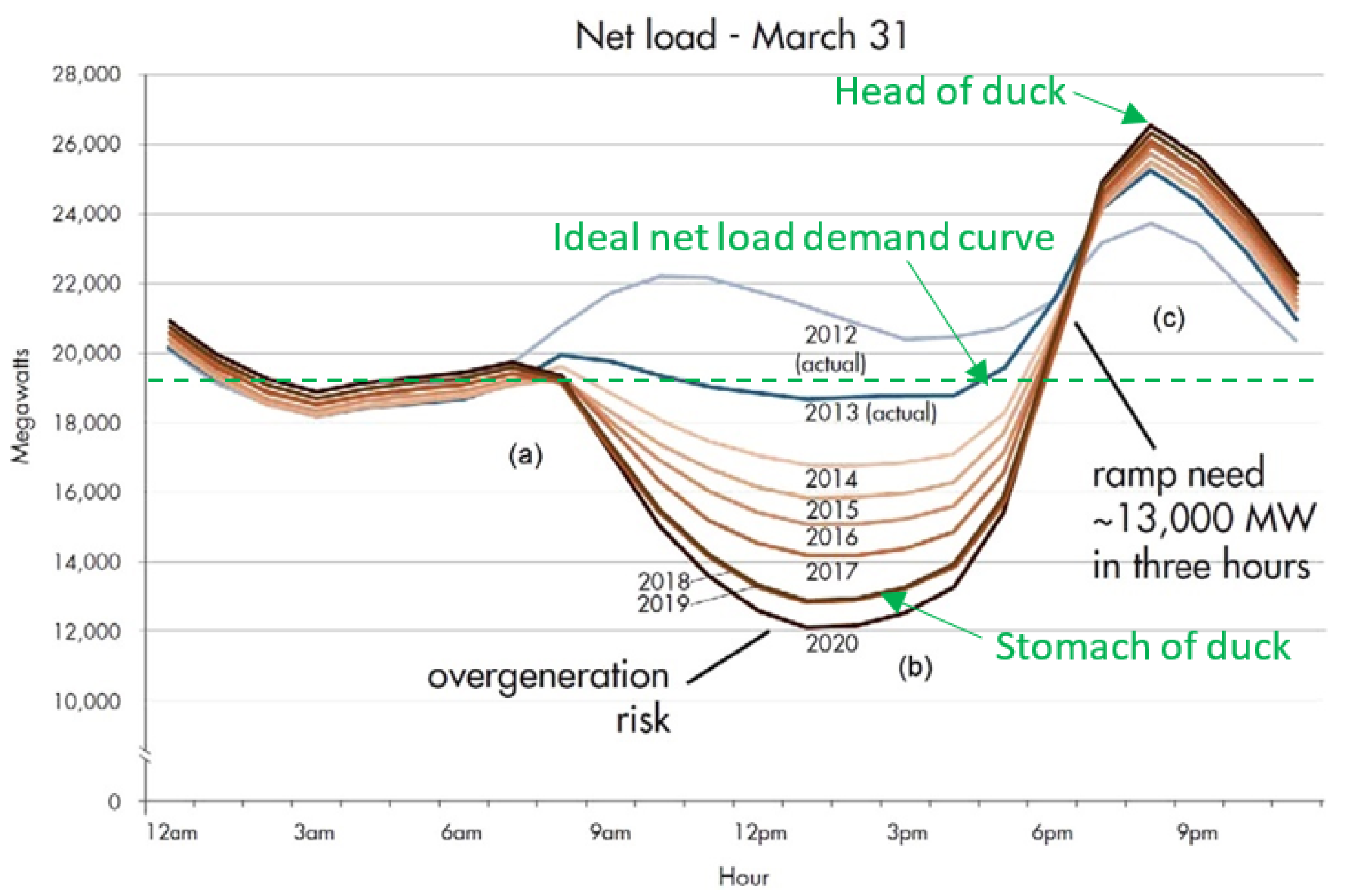
A duck-shaped curve (see in Figure 1) known as a “duck curve” has been appearing in recent years to describe the mismatch level of the grid. The duck curve (i.e., the net load demand curve) shows the total actual electricity load demand while deducting the renewable energy generation, usually PV generation [10]. When a large proportion of solar energy penetrates the grid, the duck curve becomes steeper, causing a mismatch problem (i.e., duck curve problem) between the power supply and demand sides. This problem threatens the utilization of renewable energy, energy efficiency, and the stability of power systems. Owing to the high penetration of renewable energy, the power of traditional plants, such as coal- and gas-based plants, is decreasing, resulting in an increasing number of such being considered as peak-load regulation power plants, meaning they work at low annual utilization hours and low energy efficiency. On average, the annual utilization hours decreased to 3064 h in China by 2020 [11]. Therefore, many approaches have been employed aiming to solve the duck curve problem, i.e., to smooth the net load demand curve. Widely used technologies in such approaches include demand response (DR) [12], energy storage devices [13], and power plants with variable output [5].

Figure 1.
Duck curve of California from 2012 to 2020 [14].
Demand Response (DR) is defined as “changes in electric use by demand-side resources from their normal consumption patterns in response to changes in the price of electricity or to incentive payments designed to induce lower electricity use at times of high wholesale market prices or when system reliability is jeopardized” [15]. In the aforementioned technologies, building DR has been deemed as a promising way to address the duck curve problem, owing to its considerable energy flexibility potential for building energy systems and occupant behaviors, especially for heating, ventilation, and air conditioning (HVAC) systems [4,12]. When implementing a DR program, a smart and practical DR control strategy is important. Price-based DR control strategies have been widely used in previous studies. Gohar and Mohammed [16] used a price-based control strategy to efficiently shift the peak load to a valley load time in phase change material-enhanced buildings, and other price-based DR control methods have achieved similar results [17,18,19,20]. However, price-based DR is based on a dynamic electricity price scheme that is not executed in many countries. In China, for example, the electricity market is non-liberalized and a time-of-use policy is in use; thus, incentive-based DR is the most popular DR control strategy [21]. Other advanced DR control approaches have been studied. Zhou and Zheng [22] proposed several smart DR controllers, aiming to enhance the energy flexibility of high-rise office buildings. Chapaloglou et al. [23] proposed a load pattern recognition algorithm for the peak load shaving of island-size power systems based on load forecasting.
Through the literature studies, we found that the energy flexibility capacity of buildings determines the ability and effectiveness of DR programs. Buildings with high energy flexibility have a higher degree of involvement with the grid response. The energy flexibility in buildings can be classified as either passive or active. Generally, passive flexibility systems comprise a thermal mass integrated with building HVAC systems, whereas active flexibility is based on installing extra storage devices. From an economic benefit perspective, using passive flexibility resources is cheaper and causes the initial investment and maintenance fees to be relatively low [24], whereas the initial capital costs of active approaches such as energy storage devices are relatively high. In our previous study [25], approximately 13% and 37% of the peak load could be shaved within 2 h by using a building thermal mass alone and as combined with a water storage tank for HVAC systems, respectively. Using a thermal mass and storage tank, Tang et al. [26] obtained similar results for building clusters.
Most studies for HVAC systems have focused on daily peak load reduction; for example, the common peak load time occurs at approximately 14:00–16:00 [27], and the approaches for optimizing HVAC systems to reduce peak loads have been widely studied, including approaches based on using temperature resetting, energy storage devices, and optimal controllers [22]. Windstead et al. [28] investigated the peak load reduction potential of HVAC and refrigeration systems (including 80 air handling units and 40 refrigerators) in a commercial building using a temperature resetting approach. They concluded that over 60 kW (15% of the total peak load) could be shifted. Shen et al. [29] used HVAC units of residential buildings to provide grid services. In their study, the DR load aggregator had full authority to remotely control HVAC units based on customer preferences.
Through an extensive literature review, it can be seen that the previous studies present effective results for reducing the peak load and maximizing the economic benefits of building owners; however, there remains a lack of overall analyses focusing on the purposes of bringing more renewable energy into the grid and securing the reliability of the power grid. This is owing to the following research gaps: (1) the energy flexibility capacities of buildings have not been fully used owing to the difficulty in quantifying such capacities; (2) load prediction is an important factor for optimizing building energy management, but the prediction performance is still not good enough. Therefore, further studies are required to fill these gaps.
1.2. Motivations, Innovations, and Contributions
The implementation of the optimal control of HVAC systems is based on an objective function. Traditionally, it usually takes the maximum energy savings as the objective function. However, in the context of the fast development of intermittent renewable energies in the power grid, the DR control in buildings should consider the balance of the load supply and demand side. Buildings not only need to save energy, but also need to consider the load coordinated control between the power grid and end-users at the same time. When there is a deviation between load supply and demand, how to realize the load coordinated control is important for the development of grid-interactive buildings.
The duck curve problems caused by the constant outputs of coal-fired plants impede the development of renewable energy and a sustainable society. To overcome these problems, grid-integrated buildings with advanced DR control technologies are required. Through an extensive literature review, there remains a research gap in the DR field of building HVAC systems associated with energy flexibility, e.g., from passive thermal masses and active storage tanks. To bridge this gap, we proposed two DR control strategies (rule-based and prediction-based) based on the energy flexibility quantification framework, predictive net load demand, and prediction of the day-ahead load demand. The originality and major contributions of this work are summarized as follows: (1) rule-based and prediction-based DR control strategies for smoothing the duck curves are proposed; (2) the energy flexibility resources of building thermal masses and storage tanks are quantified and considered in the DR control; and (3) a load match index is presented for evaluating the performance of DR control strategies for duck curve smoothing.
The innovation of this work includes the proposal of two coordinated DR control strategies based on the duck curve and day-ahead prediction load curve and the consideration of the energy flexibility potential. Therefore, building energy demand can be managed so as to be more coordinated with the intermittent characteristics of solar and wind energy. The results of this work could provide knowledge for energy flexibility utilization, smart building energy management, sustainable cities, and smart grid development. The remainder of this paper is structured as follows. Section 2 introduces the methodology, including the current and future duck curves of China, energy flexibility quantification framework, energy prediction approaches, and two DR control strategies. A typical office building case with central AC (Air conditioning) systems is described, modeled, and validated in Section 3. The results and discussions regarding the DR control strategies are presented in Section 4. Finally, conclusions and future work are presented in Section 5.
2. Methodology
2.1. Electricity Duck Curve in China
The shape of the duck curve (i.e., the net load demand curve) is influenced by the load demand of the end-users and the total solar electricity generation. Figure 1 illustrates the duck curve for California from 2012 to 2020 [14]. The duck curve is relatively stable during the middle of the night, decreases following sunrise in the morning, reaches the bottom at approximately noon, and reaches the peak at nightfall. With a higher penetration rate of PV energy in the grid, the duck curve becomes steeper. To solve the duck curve problems and ensure the safety of the grid, a previous study proposed three approaches [21], as follows:
- (1)
- Retrofitting a power plant’s output to be changeable. In this way, plants can work at partial load during noon, and at full load during sunset. The average output rate of coal-fired plants in China is approximately 40–100%; operation at a high output rate brings higher energy efficiency and economic benefit. The initial investment should be weighted so as to consider a broader output rate range of a coal-fired plant retrofitting program [5].
- (2)
- Implementing electricity DR. DR allows the end-users to change their load demand patterns, based on considering an electricity tariff or economic incentive [12]. In particular, the building section has massive potential as an energy flexibility resource, making it a preferable consumer for flexible energy management [27].
- (3)
- Installing energy storage devices. Energy storage is a traditional technology for managing energy demand and supply, although additional investment is required. Batteries, water tanks, and chemical storage devices are widely used.
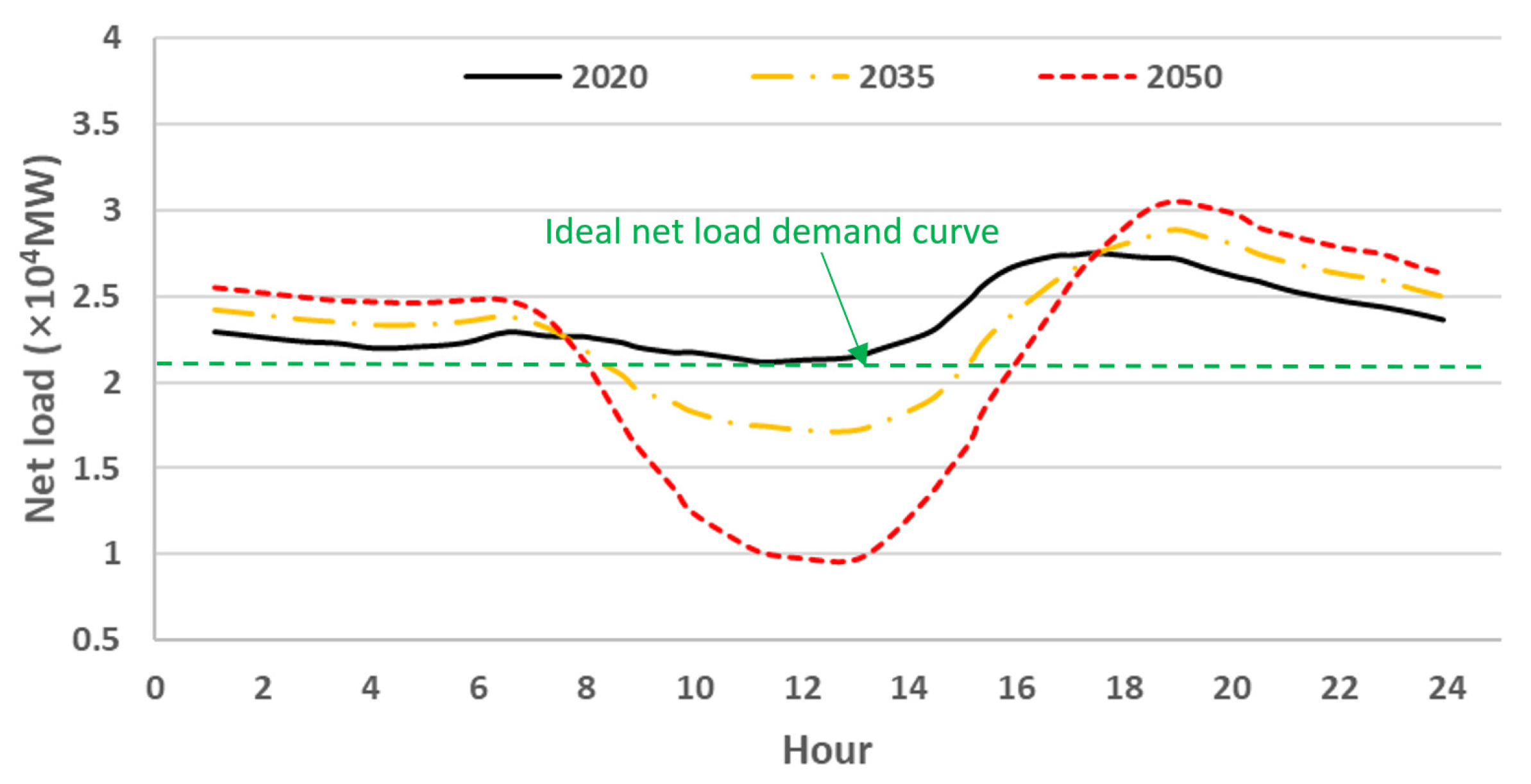
China has a different duck curve pattern than California, owing to its different energy structures. Figure 2 illustrates the predictive duck curve of North China in 2020, 2035, and 2050 [30]. There is a similar net load curve trend in other areas of China [5]. Currently, the duck curve is relatively flat since the solar energy penetration rate in the grid is not high, at approximately 11.5% (in 2020); the rate is predicted to reach 31% by 2050 [31]. With the rapid development of intermittent renewable energy sources, the duck curve will become increasingly steeper from 2020 to 2050.
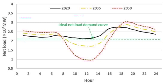
Figure 2.
Duck curve of North China in 2020, 2035, and 2050 for a typical summer day [30].
2.2. Energy Prediction Approaches
An accurate short-term load prediction to be used as a baseline is critically important for DR evaluation and DR optimal control design. Prediction strategies are usually categorized into three types: physics-based models (white box), data-driven models (black box), and reduced-order models (gray-box) [32]. Physics-based modeling tools such as EnergyPlus, Trnsys, and Dymola are widely used in the engineering industry [33]. The disadvantage of these models is that they require a significant amount of time and effort to enter the many detailed building parameters; this might be a problem for building owners, especially for buildings in the design phase. Correspondingly, data-driven models for forecasting a building’s load have been increasingly adopted, owing to their simplicity and high prediction performance. In this study, we used the Dymola software to estimate the load demand of the building case, as discussed Section 3, as an existing physics-based model was established for the DR control analysis. However, data-driven models are recommended for load demand prediction for scenarios without a ready-made physics-based model in the future practical applications.
2.3. Energy Flexibility Quantification Framework
The energy flexibility capacities of buildings are important for DR. A building with a higher electricity flexibility capacity can have a higher degree of involvement with the grid response. Thus, accurately quantifying a building’s energy flexibility before DR is useful for designing control strategies to alleviate peak loads and maximize economic benefits in DR programs. In this study, the energy flexibility of HVAC systems with and without a storage tank were investigated. The energy flexibility quantification formulas for thermal masses, HVAC systems, and storage tanks can be found in our previous works [27]. With the proposed quantification framework, the energy flexibility curves (i.e., the maximum and minimum load curves in Figure 3) were calculated, so that the load’s upward and downward capacities were known when designing the DR control strategy. Figure 3 shows the schematic diagram of energy flexibility capacity in buildings. With the existence of energy flexibility, end-users can increase power load at valley load time and reduce load at peak load time to balance the load demand. The maximum and minimum load curves could be regarded as the boundary for the DR control algorithm design.
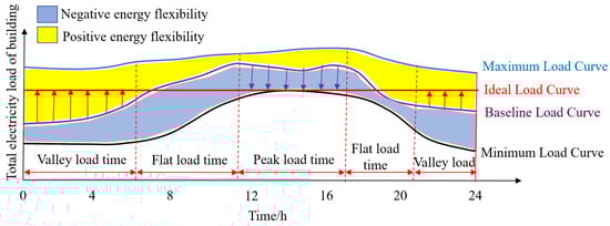
Figure 3.
Schematic diagram of energy flexibility in buildings.
2.4. Load Match Index
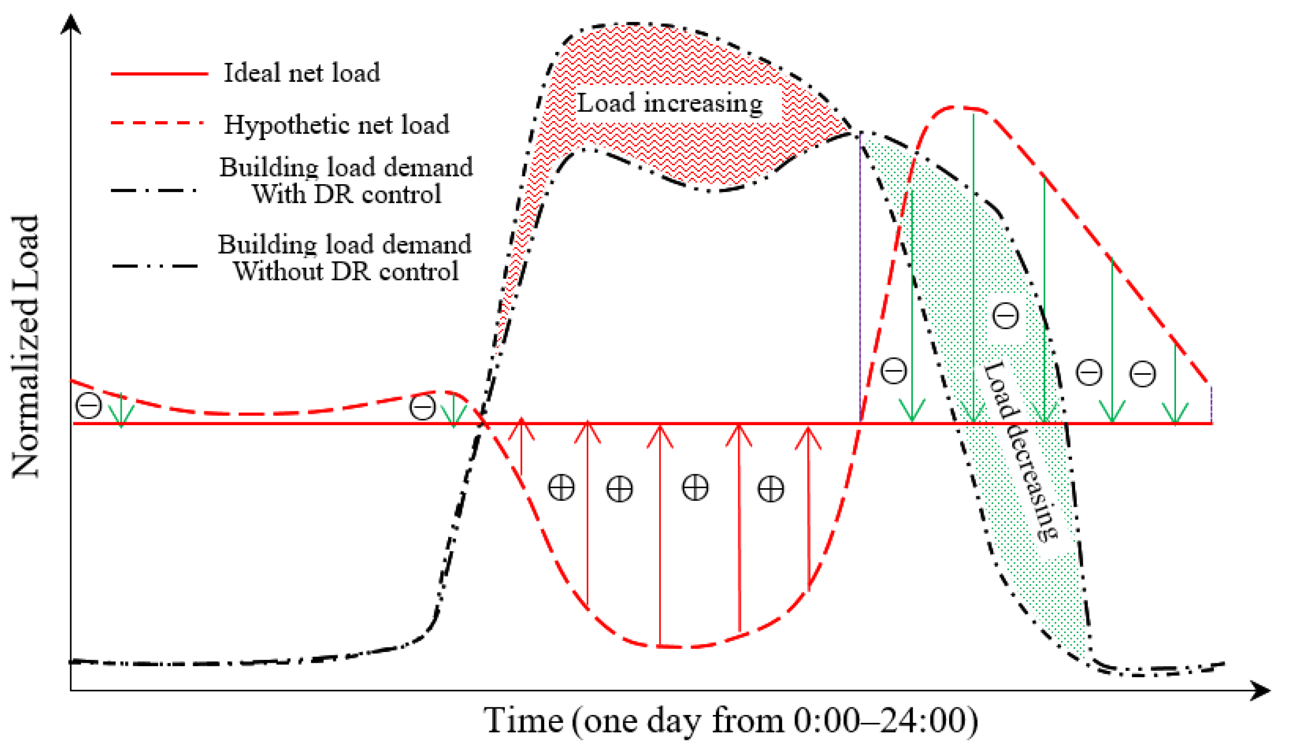
To evaluate the performance of the DR control strategies, a load match index was presented, representing the ability to increase the load demand during valley net load time while reducing the load demand during the peak net load time. Figure 4 shows the schematic diagram of the load management of different DR control strategies. The load demand of the end-users should be increased (i.e., red zone) in the “stomach” of duck curve, whereas the demand is expected to be decreased (i.e., green zone) in the “head” of duck curve. The red flat solid line represents the ideal net load line where the fossil-fired plants are easier and more effective to operate, and the red dashed line is the actual net load curve. With energy flexibility and proper DR control, buildings can shift the load demand from the “duck head” to the “duck stomach”. The load–match index is defined as shown in Equation (1), as follows:
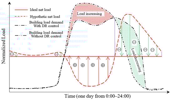
Figure 4.
Schematic diagram of the load management of different DR strategies.
In the above, represents the amount of increasing load (i.e., the area of the red zone) in the range, is the amount of the decreasing load (i.e., the area of the green zone) in the range, and is total load demand of the case without DR control. Notably, the total load demands of buildings with and without DR control may be different, and a case with DR control is generally higher than that without DR control, owing to the energy loss from energy storage devices.
2.5. Demand Response (DR) Control Strategies
The duck curves may be different in different weather/climate zones; thus, the two DR control strategies (rule-based and prediction-based) can be easily generalized for different duck curve patterns (i.e., different renewable energy penetration rate). Rule-based DR control for designing control algorithms is based on empirical data, whereas prediction-based DR control is based on day-ahead load prediction(s). In the field of DR, building loads could be classified as non-controllable, shiftable, interruptible, and adjustable loads [12]. HVAC loads are considered as adjustable loads due to the existence of the thermal comfort range, and we investigate on the adjustable HVAC loads in this paper.
The high peak load in buildings usually results from the load demand of HVAC systems. Thus, the zone temperature setting can be reset. The rule-based DR control is based on the distance between the actual and ideal net load curves. Generally, the recommended comfort temperature in buildings has a relatively large range, and these ranges vary for different building types and countries. This load distance is the decision variable and the temperature setting range is the constraint for the DR optimal control problem. The range is from 26 °C to 28 °C in the summer for office and residential buildings in China [34], and it ranges from 22.2 °C to 26.7 °C according to the American Society of Heating, Refrigerating and Air-Conditioning Engineers (ASHRAE) guidelines. Fanger’s Predicted Mean Vote (PMV) is a widely used thermal comfort index [35,36], and the comfortable range is between −0.5 and +0.5. When the zone temperature is reset to reduce or increase the HVAC loads, PMV must be satisfied. This temperature range results in buildings with an energy flexibility potential [27]. is the temperature range of the AC zone, and and are the lower and upper temperature setting limits, respectively. In addition, the load difference (, . represents the load difference of actual and ideal net load curve at the time step i, and could be minutes or hours. The temperature settings for the rule-based DR are listed in Table 1.

Table 1.
Temperature setting in the rule-based demand response (DR) control strategy.
2.5.1. Prediction-Based DR
Prediction-based DR control is based on the distance between the net load curve and predicted load curve. In this case, a predicted day-ahead building load is required. The distance can be calculated using Equation (2). The maximum distance and minimum distance are used under these conditions. The temperature settings of the prediction-based DR are listed in Table 2. Similar to rule-based DR control, the load distance is the decision variable and the temperature setting range is the constraint for the control problem.
Table 2.
Temperature setting in the prediction-based DR control.
Here, is the predicted building load (i.e., baseline), and is the ideal net load demand.
2.5.2. Control Strategy of Water Tank
In the case of HVAC systems with a storage device, buildings have higher energy flexibility [37,38]. For instance, the water tank can be charged/discharged to increase or reduce the thermal load demand so that the power demand from the chiller could be changed. In this way, the chiller can be shut off to reduce power demand and the storage tank is discharging to provide the cooling load demand during the electricity peak load time. Furthermore, the chiller can also be turned on to increase the power demand for charging the storage tank during the valley load time. To do this, we designed a control strategy for the water tank, as shown in Table 3.
Table 3.
Water tank control strategy.
3. Case Study
3.1. Office Building Description
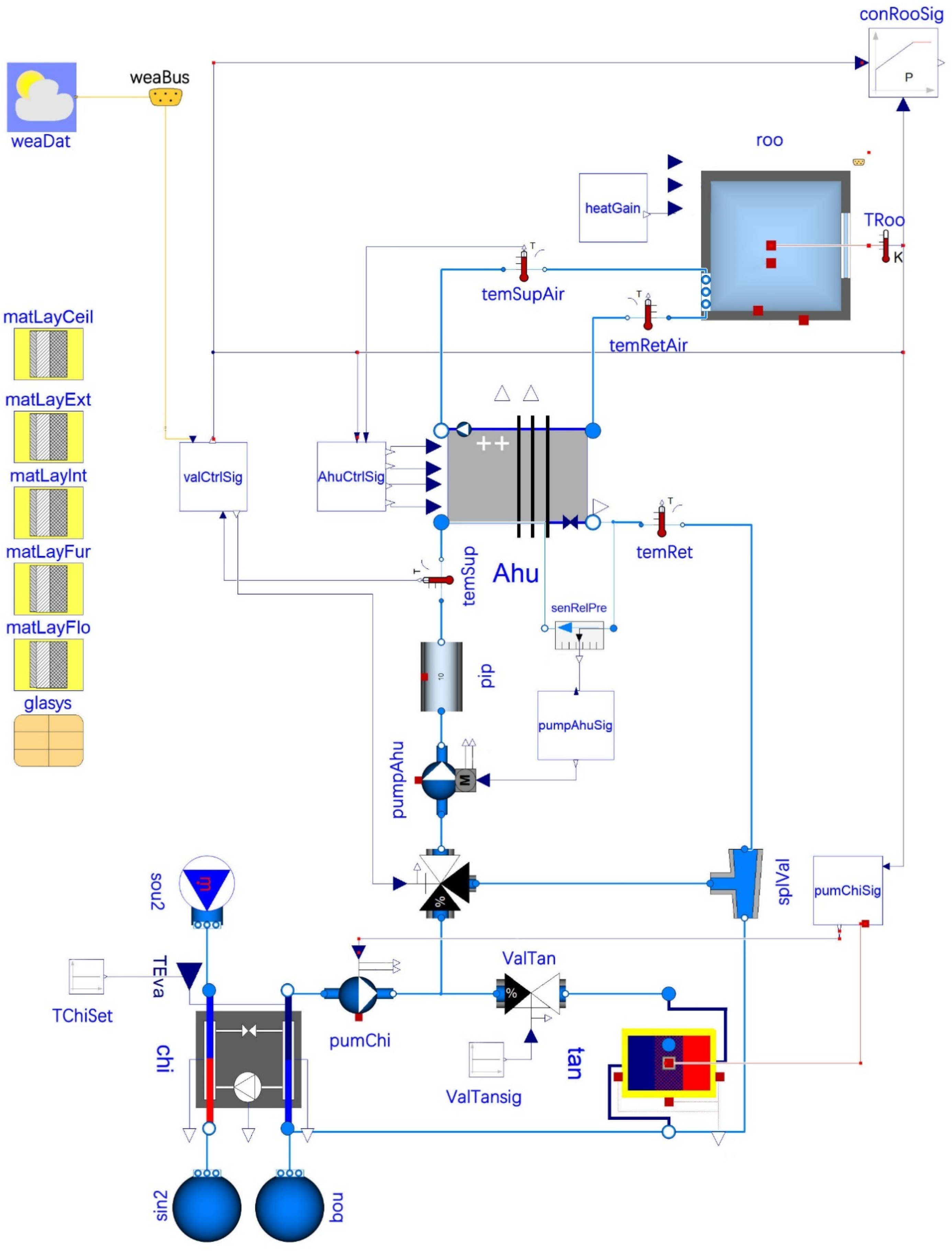
To study the performance of the different DR control strategies, a typical office building located in Shanghai, China was considered and was developed using the Modelica language on the Dymola platform. This test-bed building had 21 floors, the total building area was 51,072 m2, and the total AC area was 40,320 m2. The window-to-wall ratio was 0.33. The details of one typical office zone of this building case are listed in Table 4. The space cooling came from two central AC chillers with a design capacity of 562 kW. The main basic components selected in Dymola are listed in Table 5. Figure 5 shows the schematic layout of the air condition systems. There is a water loop by which the water storage tank is connected with the chiller directly, and it can work at several modes, including charging mode, discharging mode, and hybrid mode. In the charging mode, the chiller is working to store the chilled water in the storage tank, which usually happens at the valley load time. In the discharging mode, the storage tank provides the cooling load demand while the chiller can be shut off, which usually happens at the peak load time. In the hybrid mode, the chiller is open and the storage tank can be in the way of charging or discharging.
Table 4.
Parameters of one typical office zone.
Table 5.
Main component selection in Dymola.
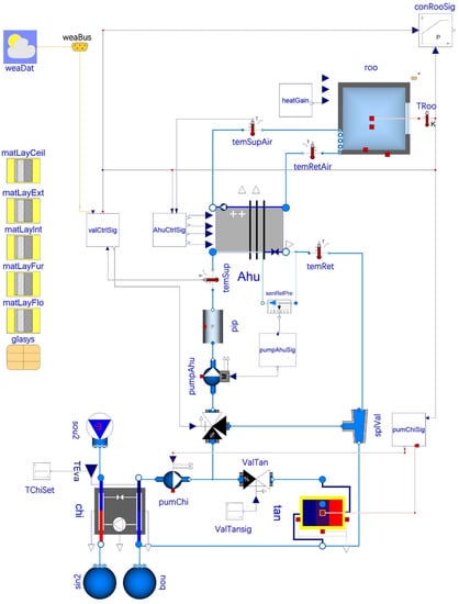
Figure 5.
Schematic layout of the air condition system in Dymola [27].
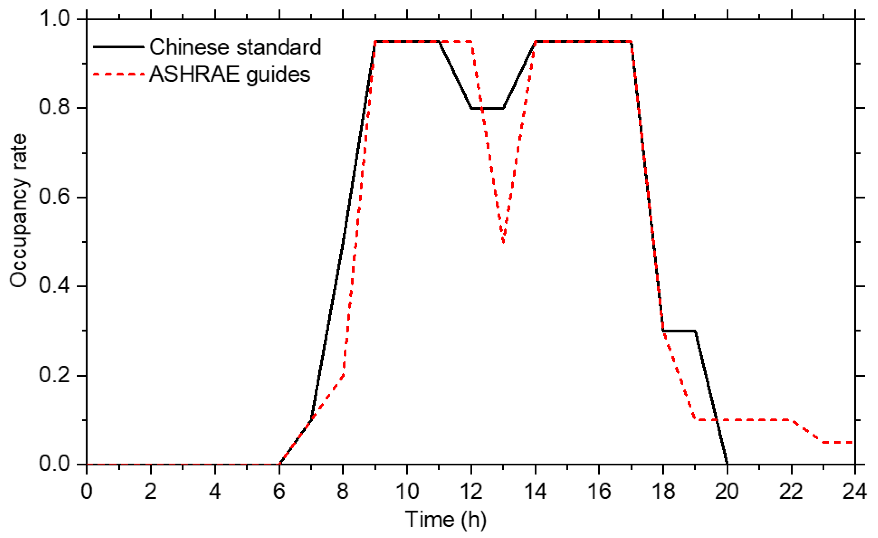
The DR control strategies considered both the energy flexibility of a passive internal thermal mass and an active storage tank. According to the national standard [39], the total internal heat gain was 40 W/m2, the light load density was 11 W/m2, and the equipment load density was 13 W/m2 for our dynamic model. The geometry of a typical office zone, detailed information of the building physics and thermophysical parameters, Modelica dynamic modeling, and model validation can be found in our previous study [27]. In addition to the building physics, which have a significant impact on the building energy use, the occupancy rate is another important factor influencing the energy consumption pattern. The occupancy rates that form the Chinese standard [39] and ASHRAE standard [40] during workdays are illustrated in Figure 6. The rate decreases at noon, owing to lunch breaks. We adopted the Chinese standard for our model. It is worth noting that accurate occupancy rates in real-time can nowadays be obtained from social media to make the building energy model more realistic [41].

Figure 6.
Occupancy rate of Chinese standard and American Society of Heating, Refrigerating and Air-Conditioning Engineers (ASHRAE) guidelines.
3.2. Energy Demand-Side Description
In our prediction-based DR strategy, accurate load prediction played an important role in improving energy management. Figure 7 shows the day-ahead electricity predicted results for a typical summer day using a physics-based Dymola model.

Figure 7.
Electricity load demand of the case study building on a typical summer day.
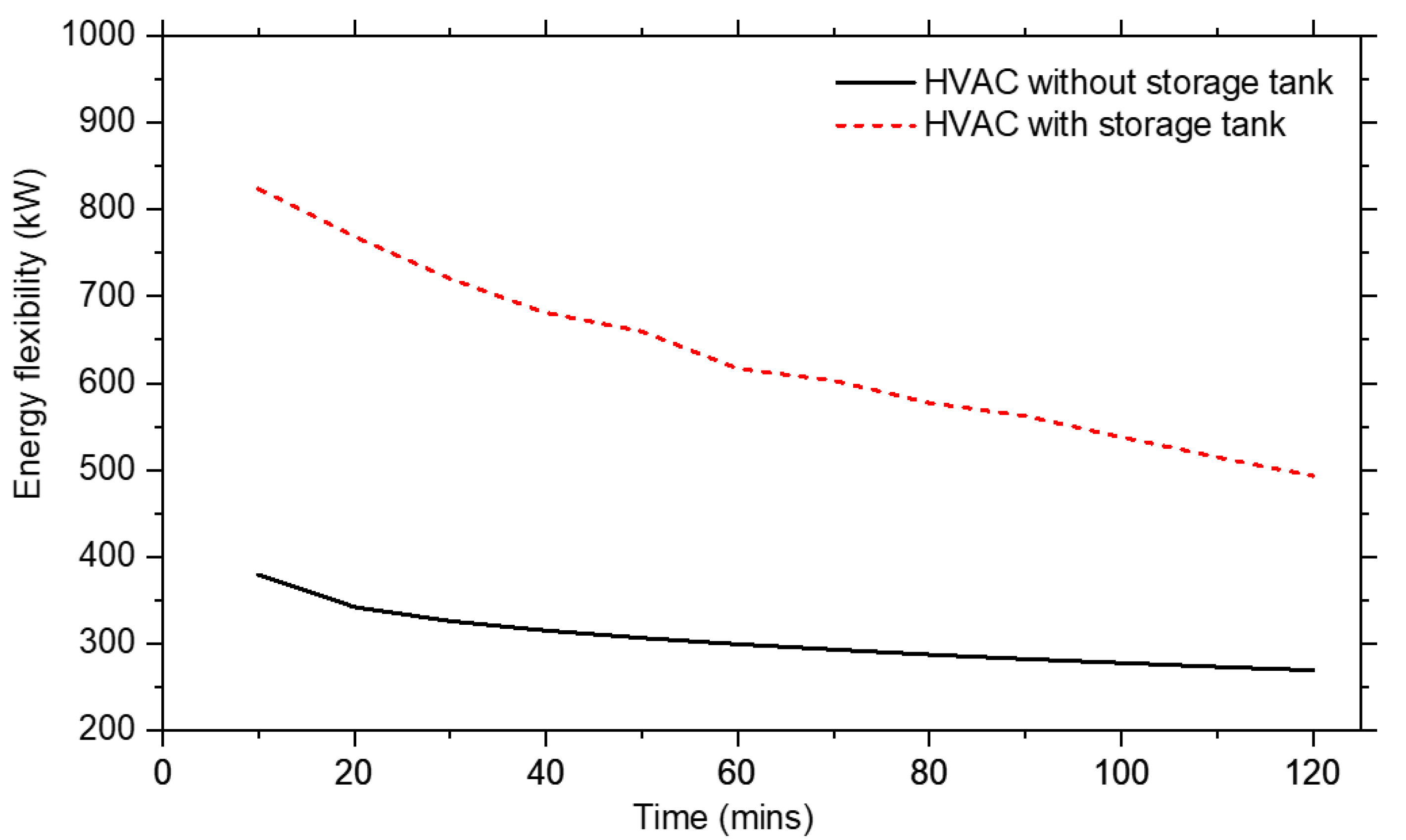
A building’s thermal flexibility resources include the passive thermal inertia of the building’s thermal mass and the active energy storage of the water tank. The energy flexibilities of the HVAC system with and without the storage tank are shown in Figure 8 by using the energy flexibility quantification framework that we proposed in our previous work [27]. The energy flexibility capacity decreases when it is used continuously. As shown in Figure 8, the flexibility capacity is high at the beginning, and is relatively low after 2 h. Usually, a common DR event does not exceed 2 h. However, the duration required to solve the duck curve problem may be longer than that of the DR event, and thus the passive energy flexibility would not be sufficient to shave the peak load and fill the valley load. Thus, an active energy-storage device is required for the buildings. In the case of a building with a storage tank, the load increase/reduction capacity is almost equal to the chiller load, since the storage tank can replace the chiller to provide cooling demand for a specific duration, indicating that the chiller can be shut off until the room temperature reaches the upper limit. Based on the flexibility curve, the DR control strategy can be optimized by considering the capacity and conditions of the energy flexibility. The energy flexibility ratios of the case study building are listed in Table 6.
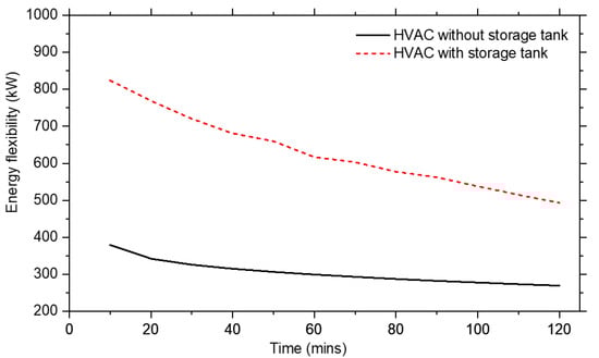
Figure 8.
Electricity flexibility of office building over 2 h.
Table 6.
Energy flexibility ratio of total building energy demand of heating, ventilation, and air conditioning (HVAC) systems with and without storage tank.
4. Results and Discussion
In this section, the results of the rule-based and prediction-based DR control strategies are analyzed for office building HVAC systems using passive and active energy flexibility. Scenario 1 represents the passive thermal mass used as an energy flexibility resource. Scenario 2 considers the active storage tank as an additional flexibility resource. One typical summer day was simulated and analyzed for these two scenarios. The simulation running time of each scenario is approximately 50 s on Dymola (Version 2018) on Windows 10, with a 2.6 GHz processor (Intel Core i7-10700) and 16 GB RAM. Notably, we show the load in a normalized manner.
4.1. Scenario 1: Passive Thermal Mass
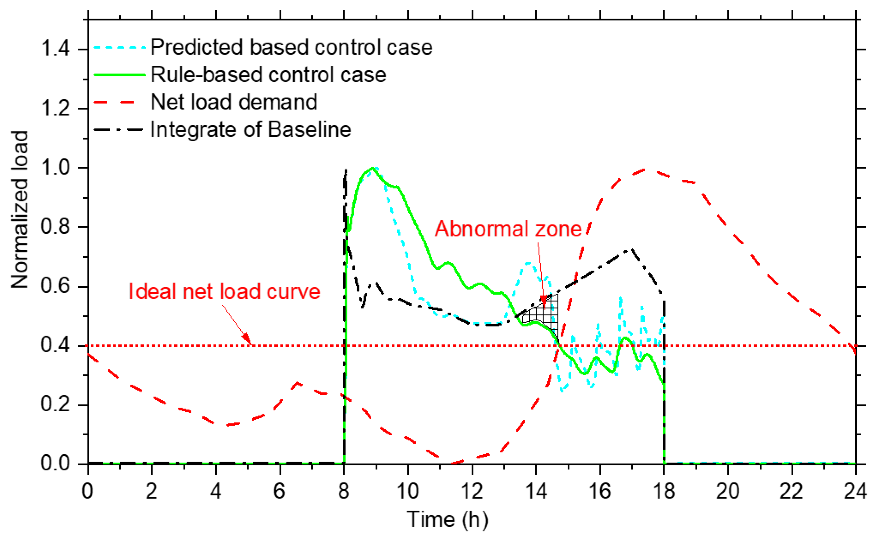
A building’s thermal masses, such as walls and furniture, comprise the main contributions to passive thermal energy flexibility; in particular, furniture has the largest flexibility and can respond quickly to provide energy flexibility. The AC was open from 8:00 to 18:00 on workdays. In our case, the temperature range is three degrees (i.e., is 24 °C and is 27 °C). A temporary peak load time occurs in the morning once the AC is switched to ON. In Figure 9, the black dash–dot line shows the baseline of the load demand, where no DR control is implemented. The green solid line and blue short dashed line represent the load demands of the rule-based and prediction-based DR control cases, respectively. Apparently, compared with the baseline, the load demand is increased in the morning and decreases in the afternoon, owing to the DR control. Thus, the net load demand can be flattened. The load match indices are 0.38 and 0.24 for rule-based and prediction-based DR control, respectively. In addition, the load demand of the rule-based case is decreased where it is expected to increase, which is referred to as the “abnormal zone” in Figure 9. Although the load match index is higher in the rule-based case, the abnormal zone appears, which degrades the ability and overall performance of smoothing the net load curve.
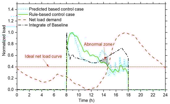
Figure 9.
Normalized load curve of rule-based and prediction-based demand response (DR) control in Scenario 1.
4.2. Scenario 2: Passive Thermal Mass + Water Storage Tank
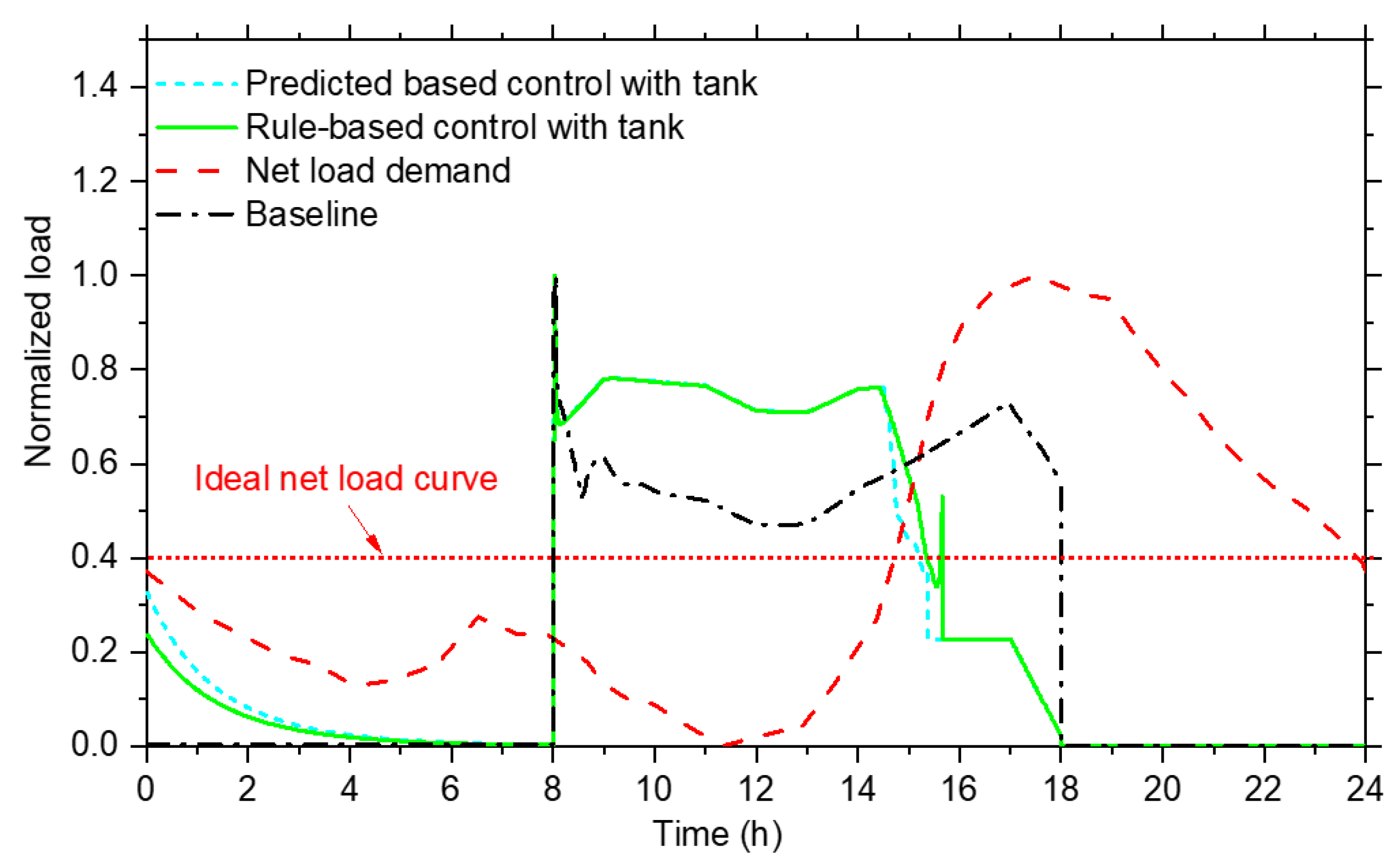
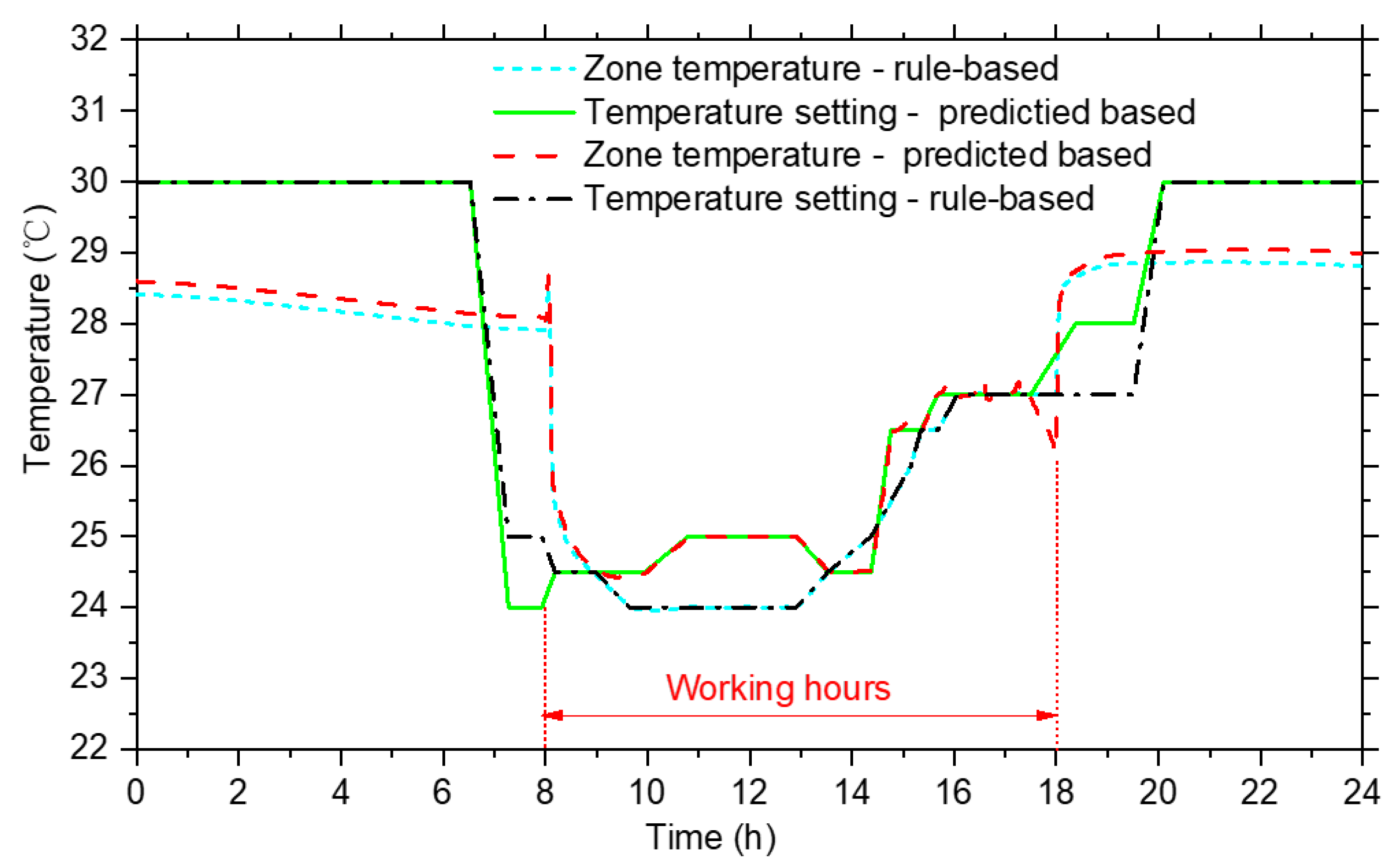
To increase the ability to smooth the net load curve, the water storage tank is integrated into the HVAC systems, and the results are shown in Figure 10. The load match indices are 0.51 and 0.55 by using the approach proposed in Section 2.4 for the rule-based and prediction-based control, respectively. Compared with the case without a storage tank, Scenario 2 can shift more loads from valley to peak load times. Furthermore, the net load can be increased in the middle of the night, owing to the recharging of the storage tank. Figure 11 shows the temperature setting and real-time zone temperatures from the proposed DR controls. The real-time zone temperature meets the set value in both cases.
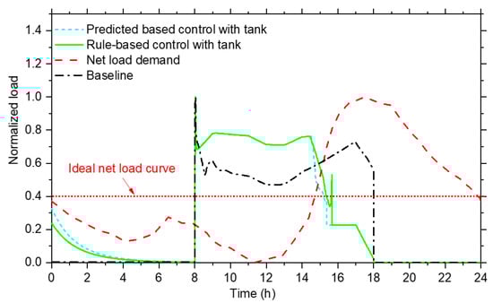
Figure 10.
Normalized load curve of rule-based and prediction-based DR control in Scenario 2.

Figure 11.
Temperature setting and real-time zone temperature of the two proposed control strategies.
4.3. Discussion
Currently, three-tiered electricity tariffs are the mainstream in China and are usually divided into three different tariffs for peak, flat, and valley load times [42]. With this electricity price policy, energy storage devices are generally charged using cheap valley electricity in the middle of the night, and are discharged at high peak electricity tariff times. As shown in Figure 1, in the future power grid, the bottom of the duck curve appears at noon when the solar energy generation reaches its peak, indicating that the power grid is at a surplus and that more electricity is expected to be consumed at noon rather than during the middle of the night, as before. Thus, the existing electricity tariff schemes in China hinder the penetration of solar energy into the grid. Under these conditions, the future price scheme should be based on the shortages or surpluses of power grids affected by intermittent renewable energies. For example, the electricity price is low at the bottom of the duck curve (i.e., the range in Figure 4) and is relatively high at the head of the duck curve (i.e., the range in Figure 4). Thus, multiple-tired or dynamic tariffs could be adopted to solve the duck problem.
The use of passive energy flexibility is almost free, except for some additional investment for smart meters. The utilization of a water storage tank requires a considerable initial investment, but the energy’s flexible ability is upgraded, and the break-even point is relatively short. Thus, HVAC systems with storage tanks are recommended for providing high penetration of renewable energy in the grid. As shown in Table 6, the upward and downward energy flexibility capacities are approximately 33.8% and 42.0% of the total building load at the beginning for Scenarios 1 and 2, respectively. As shown in Figure 9 and Figure 10, the energy’s flexibility potential is fully used at 8:00 am, whereafter, the upward capacity decreases with the consumption of energy flexibility, and the upward capacity reaches the bottom limit at noon. In Scenario 1, the control strategy fully utilizes the energy flexibility potential. In Scenario 2, the used upward energy flexibility is approximately 30.0% in the morning, but 42.0% exists, indicating that further upward loads can be achieved. Compared with the energy flexibility capacity in Table 6, it can be seen that there is still some energy flexibility not being fully used.
For the rule-based control case, as shown in Figure 9, the existence of an “abnormal zone” degrades the ability of load shifting. Thus, this zone could be avoided by designing a better rule-based DR control strategy. The temperature setting in Table 1 could be optimized, for instance, temperature could be set lower to increase the power demand during the abnormal zone time. For the prediction-based control case, the “abnormal zone” problem disappears, which means that the prediction-based control is better, despite the fact that the predicted load baseline is additionally required. As shown in Figure 9, meanwhile, the peak load of the case building can be shifted by 24–38% using only the energy flexibility capacity of passive thermal mass, and this rate could reach 51–55% when an active storage tank is integrated, without sacrificing the occupant’s comfort. In paper [43], 25% of peak load reduction can be achieved by a 2 °C higher than normal thermostat setting in the cooling demand season. Similar results of 18.7% to 39.0% have been found in several other papers [44,45,46].
In addition, providing pre-cooling/heating before peak load occurrence has been validated as an effective approach to reducing the peak load demands of HVAC systems [25,47]. For example, in a cooling supply case, pre-cooling usually occurs in the middle of the night, and the temperature setting can be low, i.e., up to 20 °C [48]. In this way, the temperature setting can be set to a low value in the range in Figure 4 and to a high value in the range to achieve higher energy flexibility. To avoid the discomfort caused by temperature changes, some pre-cooling strategies can be used, such as linear, exponential, and stepping temperature resetting [49].
In this study, we investigate the load smoothing ability of an office building, and its operation time usually corresponds to the period of the solar energy supply. When the solar energy supply ends at dusk, the energy demands of office buildings are also offloaded, whereas the energy demands of residential buildings increase, leading to their peak loads at dusk. Thus, residential buildings are promising customers for providing DR resources. With the wide working time window for electrical appliances, such as washing machines, dishwashers, and electric vehicles, residential buildings have massive energy flexibility potential [50] and can play important roles as grid-integrated buildings.
5. Conclusions
In this paper, two DR control strategies are proposed, considering a building’s energy flexibility capacity to solve duck curve problems. Specifically, the rule-based DR strategy is based on the distance between the actual and ideal net load curve; the prediction-based DR strategy is based on the distance between the net load curve and day-ahead load prediction curve (i.e., baseline). These two proposed strategies can be integrated into building energy management systems in practical applications. The energy flexibility abilities of the building thermal mass and water storage tank are quantified using our previous quantification framework. The load match index is presented to evaluate the performance of these two DR control strategies. The results show that 24–38% of a building’s total load can be shifted from the peak load time to valley load time using only the passive thermal mass, and that this rate could reach 51–55% when an active storage tank is integrated. In addition, the results show that the prediction-based DR control strategy outperforms the rule-based DR control in regard to smoothing the net load curve, although an accurate day-ahead load forecasting curve is required.
This work provides a reference basis for smart grid-integrated building energy management in the context of the high penetration rate of renewable energies in the modern power grid. The proposed DR control strategies can be applied to public buildings and generalized to other building types, such as residential buildings. The net load curve is being reshaped with increasingly intermittent renewable energy penetrating the power grid; therefore, load aggregators can integrate all of the flexibility resources to coordinate the supply from the power grid and the demand from end-users, and building owners can benefit from participating in DR programs. As the peak load time of the grid is moved to dusk, future works are expected to consider DR control strategies based on the energy flexibility of electric appliances in residential buildings, including washing machines, dishwashers, electric vehicles, and AC, which commonly work at night when residents come home from office buildings. In the future of building energy systems, DR control strategies will not only consider the total energy savings but also energy supply–demand coordination in the objective function. For instance, when the power grid is jeopardized because of supply–demand balance problems, buildings can respond by increasing or decreasing power consumption simultaneously according to the load supply–demand conditions for the sake of the power grid’s stability and safety. To do that, an optimal DR control strategy considering the energy flexibility capacity of buildings and supply–demand coordination of the power grid should be developed in future energy markets.
Author Contributions
Conceptualization, Y.C.; methodology, Y.C.; software, Z.C.; writing—original draft preparation, Y.C.; writing—review and editing, X.Y., L.S. and K.L.; visualization, Z.C.; funding acquisition, Y.C. and K.L. All authors have read and agreed to the published version of the manuscript.
Funding
This research was funded by China Postdoctoral Science Foundation grant number 2020M681347 and the National Nature Science Foundation of China grant number 51906158. And the APC was funded by China Postdoctoral Science Foundation.
Institutional Review Board Statement
Not applicable.
Informed Consent Statement
Not applicable.
Data Availability Statement
Not applicable.
Acknowledgments
This work was funded by the China Postdoctoral Science Foundation (No. 2020M681347) and National Nature Science Foundation of China (No. 51906158).
Conflicts of Interest
The authors declare no conflict of interest.
References
- Blueprint for China’s New Growth Story, China Daily Global. Available online: https://global.chinadaily.com.cn/a/202102/01/WS60174a18a31024ad0baa64e9.html (accessed on 9 March 2022).
- Peng, M.; Xu, H.; Qu, C.; Xu, J.; Chen, L.; Duan, L.; Hao, J. Understanding China’s largest sustainability experiment: Atmospheric and climate governance in the Yangtze River economic belt as a lens. J. Clean. Prod. 2021, 290, 125760. [Google Scholar] [CrossRef]
- Cheng, Y.; Yao, X. Carbon intensity reduction assessment of renewable energy technology innovation in China: A panel data model with cross-section dependence and slope heterogeneity. Renew. Sustain. Energy Rev. 2021, 135, 110157. [Google Scholar] [CrossRef]
- Sheha, M.; Mohammadi, K.; Powell, K. Solving the duck curve in a smart grid environment using a non-cooperative game theory and dynamic pricing profiles. Energy Convers. Manag. 2020, 220, 113102. [Google Scholar] [CrossRef]
- Hou, Q.; Zhang, N.; Du, E.; Miao, M.; Peng, F.; Kang, C. Probabilistic duck curve in high PV penetration power system: Concept, modeling, and empirical analysis in China. Appl. Energ. 2019, 242, 205–215. [Google Scholar] [CrossRef]
- The Texas Blackout is the Story of a Disaster Foretold. Available online: https://www.texasmonthly.com/politics/texas-blackout-preventable/ (accessed on 9 March 2022).
- O’Shaughnessy, E.; Cruce, J.R.; Xu, K. Too much of a good thing? Global trends in the curtailment of solar PV. Sol. Energy 2020, 208, 1068–1077. [Google Scholar] [CrossRef]
- Qi, Y.; Dong, W.; Dong, C.; Huang, C. Understanding institutional barriers for wind curtailment in China. Renew. Sustain. Energy Rev. 2019, 105, 476–486. [Google Scholar] [CrossRef]
- Online Press Conference of First-Quarter 2021, National Energy Administration. Available online: http://www.nea.gov.cn/2021-01/30/c_139708580.htm (accessed on 16 March 2022).
- California Independent System Operator. What the Duck Curve Tells Us about Managing a Green Grid. Available online: http://large.stanford.edu/courses/2015/ph240/burnett2/docs/flexible.pdf (accessed on 16 March 2022).
- Statistics of China Power 2020. (In Chinese). Available online: https://pdf.dfcfw.com/pdf/H3_AP202011201431357398_1.pdf?1605888067000.pdf (accessed on 16 March 2022).
- Chen, Y.; Xu, P.; Gu, J.; Schmidt, F.; Li, W. Measures to improve energy demand flexibility in buildings for demand response (DR): A review. Energy Build. 2018, 177, 125–139. [Google Scholar] [CrossRef]
- Meng, Q.; Li, Y.; Ren, X.; Xiong, C.; Wang, W.; You, J. A demand-response method to balance electric power-grids via HVAC systems using active energy-storage: Simulation and on-site experiment. Energy Rep. 2021, 7, 762–777. [Google Scholar] [CrossRef]
- Obi, M.; Bass, R. Trends and challenges of grid-connected photovoltaic systems – A review. Renew. Sustain. Energy Rev. 2016, 58, 1082–1094. [Google Scholar] [CrossRef]
- Federal Energy Regulation Commission. 2010 Assessment of Demand Response and Advanced Metering; United States Department of Energy: Washington, DC, USA, 2011.
- Gholamibozanjani, G.; Farid, M. Peak load shifting using a price-based control in PCM-enhanced buildings. Sol. Energy 2020, 211, 661–673. [Google Scholar] [CrossRef]
- Lu, R.; Bai, R.; Huang, Y.; Li, Y.; Jiang, J.; Ding, Y. Data-driven real-time price-based demand response for industrial facilities energy management. Appl. Energy 2021, 283, 116291. [Google Scholar] [CrossRef]
- Rajamand, S. Effect of demand response program of loads in cost optimization of microgrid considering uncertain parameters in PV/WT, market price and load demand. Energy. 2020, 194, 116917. [Google Scholar] [CrossRef]
- Huang, P.; Xu, T.; Sun, Y. A genetic algorithm based dynamic pricing for improving bi-directional interactions with reduced power imbalance. Energy Build. 2019, 199, 275–286. [Google Scholar] [CrossRef]
- Yan, X.; Ozturk, Y.; Hu, Z.; Song, Y. A review on price-driven residential demand response. Renew. Sustain. Energy Rev. 2018, 96, 411–419. [Google Scholar] [CrossRef]
- Chen, Y.; Zhang, L.; Xu, P.; Di Gangi, A. Electricity demand response schemes in China: Pilot study and future outlook. Energy 2021, 224, 120042. [Google Scholar] [CrossRef]
- Zhou, Y.; Zheng, S. Machine-learning based hybrid demand-side controller for high-rise office buildings with high energy flexibilities. Appl. Energy 2020, 262, 114416. [Google Scholar] [CrossRef]
- Chapaloglou, S.; Nesiadis, A.; Iliadis, P.; Atsonios, K.; Nikolopoulos, N.; Grammelis, P.; Yiakopoulos, C.; Antoniadis, I.; Kakaras, E. Smart energy management algorithm for load smoothing and peak shaving based on load forecasting of an island’s power system. Appl. Energy 2019, 238, 627–642. [Google Scholar] [CrossRef]
- Jarvinen, J.; Goldsworthy, M.; White, S.; Pudney, P.; Belusko, M.; Bruno, F. Evaluating the utility of passive thermal storage as an energy storage system on the Australian energy market. Renew. Sustain. Energy Rev. 2021, 137, 110615. [Google Scholar] [CrossRef]
- Chen, Y.; Xu, P.; Chen, Z.; Wang, H.; Sha, H.; Ji, Y.; Zhang, Y.; Dou, Q.; Wang, S. Experimental investigation of demand response potential of buildings: Combined passive thermal mass and active storage. Appl. Energy 2020, 280, 115956. [Google Scholar] [CrossRef]
- Tang, R.; Li, H.; Wang, S. A game theory-based decentralized control strategy for power demand management of building cluster using thermal mass and energy storage. Appl. Energy 2019, 242, 809–820. [Google Scholar] [CrossRef]
- Chen, Y.; Chen, Z.; Xu, P.; Li, W.; Sha, H.; Yang, Z.; Li, G.; Hu, C. Quantification of electricity flexibility in demand response: Office building case study. Energy 2019, 188, 116054. [Google Scholar] [CrossRef]
- Winstead, C.; Bhandari, M.; Nutaro, J.; Kuruganti, T. Peak load reduction and load shaping in HVAC and refrigeration systems in commercial buildings by using a novel lightweight dynamic priority-based control strategy. Appl. Energy 2020, 277, 115543. [Google Scholar] [CrossRef]
- Shen, Y.; Li, Y.; Zhang, Q.; Shi, Q.; Li, F. State-shift priority based progressive load control of residential HVAC units for frequency regulation. Electr. Power Syst. Res. 2020, 182, 106194. [Google Scholar] [CrossRef]
- State Grid Energy Research Institute. China Energy & Electricity Outlook 2019; China Electric Power Press: Beijing, China, 2019. (In Chinese) [Google Scholar]
- National Energy Administration, National Power Statistics. (In Chinese). Available online: http://www.nea.gov.cn/2021-01/20/c_139683739.htm (accessed on 16 March 2022).
- Luo, X.J.; Oyedele, L.O.; Ajayi, A.O.; Akinade, O.O.; Owolabi, H.A.; Ahmed, A. Feature extraction and genetic algorithm enhanced adaptive deep neural network for energy consumption prediction in buildings. Renew. Sustain. Energy Rev. 2020, 131, 109980. [Google Scholar] [CrossRef]
- Nageler, P.; Schweiger, G.; Pichler, M.; Brandl, D.; Mach, T.; Heimrath, R.; Schranzhofer, H.; Hochenauer, C. Validation of dynamic building energy simulation tools based on a real test-box with thermally activated building systems (TABS). Energy Build. 2018, 168, 42–55. [Google Scholar] [CrossRef]
- Lu, Y.; Ma, Z.; Zou, P. Heating, Ventilation and Air Conditioning (In Chinese); China Building Industry Press: Beijing, China, 2014. [Google Scholar]
- Carli, R.; Cavone, G.; Dotoli, M.; Epicoco, N.; Scarabaggio, P. Model predictive control for thermal comfort optimization in building energy management systems. In Proceedings of the 2019 IEEE International Conference on Systems, Man and Cybernetics (SMC), Bari, Italy, 6–9 October 2019. [Google Scholar]
- Klauco, M.; Kvasnica, M. Explicit MPC approach to PMV-based thermal comfort control. In Proceedings of the 53rd IEEE Conference on Decision and Control, Los Angeles, CA, USA, 15–17 December 2014. [Google Scholar]
- Carli, R.; Cavone, G.; Pippia, T.; Schutter, B.D.; Dotoli, M. A Robust MPC Energy Scheduling Strategy for Multi-Carrier Microgrids. In Proceedings of the 2020 IEEE 16th International Conference on Automation Science and Engineering (CASE), Hong Kong, China, 20–21 August 2020. [Google Scholar]
- Iver, B.S.; Magnus, K. Energy Storage Scheduling in Distribution Systems Considering Wind and Photovoltaic Generation Uncertainties. Energies 2019, 12, 1231. [Google Scholar]
- Design Standard for Energy Efficiency of Public Buildings; Ministry of Housing and Urban-Rural Development of the People’s Republic of China: Beijing, China, 2015. (In Chinese)
- Labeodan, T.; Zeiler, W.; Boxem, G.; Zhao, Y. Occupancy measurement in commercial office buildings for demand-driven control applications—A survey and detection system evaluation. Energy Build. 2015, 93, 303–314. [Google Scholar] [CrossRef] [Green Version]
- Lu, X.; Feng, F.; Pang, Z.; Yang, T.; Zheng, O.N. Extracting typical occupancy schedules from social media (TOSSM) and its integration with building energy modeling. Build. Simul. 2020, 14, 25–41. [Google Scholar] [CrossRef]
- Retail Electricity Tarrif in Shanghai. Available online: http://fgw.sh.gov.cn/jgl/20201201/4137ad5b6a10415fbe569958f5959987.html (accessed on 15 October 2021). (In Chinese)
- Aduda, K.O.; Labeodan, T.; Zeiler, W.; Boxem, G.; Zhao, Y. Demand side flexibility: Potentials and building performance implications. Sustain. Cities Soc. 2016, 22, 146–163. [Google Scholar] [CrossRef]
- Wang, S.; Gao, D.; Tang, R.; Xiao, F. Cooling Supply-based HVAC System Control for Fast Demand Response of Buildings to Urgent Requests of Smart Grids. Energy Procedia 2016, 103, 34–39. [Google Scholar] [CrossRef]
- Cui, B.; Wang, S.; Yan, C.; Xue, X. Evaluation of a fast power demand response strategy using active and passive building cold storages for smart grid applications. Energy Convers. Manag. 2015, 102, 227–238. [Google Scholar] [CrossRef]
- Palacio, S.N.; Valentine, K.F.; Wong, M.; Zhang, K.M. Reducing power system costs with thermal energy storage. Appl. Energy 2014, 129. [Google Scholar]
- Turner, W.J.N.; Walker, I.S.; Roux, J. Peak load reductions: Electric load shifting with mechanical pre-cooling of residential buildings with low thermal mass. Energy 2015, 82, 1057–1067. [Google Scholar] [CrossRef]
- Xu, P.; Chen, Y.; Li, W.; Chen, Z.; Wang, H.; Chen, Z. Building Demand Response Control and Applications (In Chinese); China Building Industry Press: Beijing, China, 2020. [Google Scholar]
- Sun, Y.; Wang, S.; Xiao, F.; Gao, D. Peak load shifting control using different cold thermal energy storage facilities in commercial buildings: A review. Energy Convers. Manag. 2013, 71, 101–114. [Google Scholar] [CrossRef]
- D’Hulst, R.; Labeeuw, W.; Beusen, B.; Claessens, S.; Deconinck, G.; Vanthournout, K. Demand response flexibility and flexibility potential of residential smart appliances: Experiences from large pilot test in Belgium. Appl. Energy 2015, 155, 79–90. [Google Scholar] [CrossRef]


Publisher’s Note: MDPI stays neutral with regard to jurisdictional claims in published maps and institutional affiliations. |
© 2022 by the authors. Licensee MDPI, Basel, Switzerland. This article is an open access article distributed under the terms and conditions of the Creative Commons Attribution (CC BY) license (https://creativecommons.org/licenses/by/4.0/).