Abstract
In this paper, a previous experimental investigation on physical refining of steel melts by filtration was numerically studied. To be specific, the filtration of non-metallic alumina inclusions, in the size range of 1–100 µm, was stimulated from steel melt using a square-celled monolithic alumina filter. Computational fluid dynamics (CFD) studies, including simulations of both fluid flow and particle tracing using the one-way coupling method, were conducted. The CFD predicted results for particles in the size range of ≤5 µm were compared to the published experimental data. The modeled filtration setup could capture 100% of the particles larger than 50 µm. The percentage of the filtered particles decreased from 98% to 0% in the particle size range from 50 µm to 1 µm.
1. Introduction
In metallurgy, ceramic filters are used to remove solid particles and inclusions from molten metals [1,2,3,4]. Inclusions play an important role in the mechanical properties of metallic materials [4,5,6,7,8,9,10,11]. Sometimes, they are intentionally generated, carefully controlled, and quantified, i.e., inclusion engineering, to create a specific type of material with desired mechanical properties [9,12]. However, most of the time, the main aim is to remove, control, and/or decrease the number of unwanted inclusions [4,6,7,10,13]. Many well-known and established techniques are used to satisfy this aim [7,10,14]. However, there is still an interest in deeper understanding the mechanisms of the formation and behavior of inclusions in molten metal and in developing more effective methods which would be practical, simple, and cost-efficient [6,10,13,15] to remove inclusions from molten metal.
The physical removal of inclusions from molten metal is a well-known phenomenon in the production of non-ferrous metals. Particularly, numerous research projects have been conducted, and several filtration methods have been developed in the aluminum industry [16,17,18,19]. However, few published research works on the physical filtration of molten steel are available. In general, the demand for high-quality steel requires the removal and control of non-metallic inclusions [5,8,9,10,13,16,20]. The volume fraction of non-metallic inclusions depends mainly on the oxygen and sulphur contents of the steel melt [5,9,13,21]. These two elements are generally present as oxides and sulphides in the steel melts and form non-metallic inclusions [5,9,10,13,15]. To reduce the dissolved oxygen content, deoxidizers such as Al, Fe-Al, Ti, Fe-Si, Fe-Ti, etc. are added to the steel melt [13,20,22,23,24]. The products of the deoxidization process are various sizes and types of inclusions [13,25]. A fraction of the inclusions is removed during the slag refining process. However, the small inclusions could remain in the steel melt and move along the direction of the bulk flow of the molten steel [13,26,27]. There, collisions between the inclusions occur, which result in the agglomeration and clustering of alumina inclusions [13,22,25,28]. Among non-metallic inclusions, the deposition of alumina inclusions in tundish nozzles is believed to cause reduced molten steel pouring rate and nozzle blockage [10,13,22,25,26,29,30] while teeming the tundish from steel melts during castings. In addition to the submerged entry nuzzle and/or tundish nuzzle, such blockage may occur in the ladle shroud as well [31,32,33]. Therefore, there has been great interest in finding a practical and inexpensive technique to remove or reduce the amount of these inclusions prior to casting and/or while casting [30,31].
In 1985, S. Ali et al. [10,13,15] performed several laboratory-scale molten steel filtration experiments targeting alumina inclusions that were 5 µm and smaller. In their experiment, two types of filters were used: (a) tabular granules of alumina and (b) monolithic extruded alumina. It was shown that it is possible to physically remove alumina inclusions with both types of filters. To be specific, it was revealed that lower molten steel flow rates and increased filter heights/lengths escalated the inclusion removal efficiency.
In 1991, K. Uemura et al. [16] used ceramic loop filters of different ceramic materials as well as different string diameters to physically remove alumina inclusions and to study the filtration mechanisms. They found that the filter material had no significant effect on the filtration efficiency. It was also found that the filtration efficiency depended on the string diameter and initial oxygen content. The highest filtration efficiency could be achieved using a 2 mm diameter string filter media. Here, inclusions in the size range greater than 5 µm were reduced by filtration.
In 2012, L. Bulkowski et al. [34] performed both laboratory- and industrial-scale molten steel filtration experiments. They used ceramic corundum and mullite as filter materials. For the laboratory test, it was reported that the surface share of inclusions in filtered steel was reduced by 48–50% compared to the unfiltered steel. The total oxygen content and number of inclusions were reduced by 58% and 38%, respectively. In addition, the industrial tests were carried out during the downhill casting of the molten steel into molds. Here, the maximum surface share of the inclusions and number of inclusions were reduced by 33% and 13% respectively. The overall decrease in the oxygen content was also reported to reach a maximum of 75%.
Recently, S. Chakraborty et al. [35,36] used 10 Pore Per Inch (PPI) MgO-stabilized zirconia foam filters to study the filtration efficiency of solid alumina inclusions from molten steel. The highest overall inclusion efficiency achieved by filtration, while comparing castings produced with and without a filter from the same heat, was reported to be 48%.
The current research aims at developing a reliable computational fluid dynamics (CFD) model to predict the filtration of inclusions from molten steel. To validate the CFD model, the experimental work on the physical refining of steel melt using monolithic extruded alumina filters by S. Ali et al. [10,13,15] was used.
2. Theoretical Background
Summary of the Physical Steel Melt Refining Experiments
S. Ali et al. designed an experimental apparatus and a filter setup and used square-celled monolithic extruded alumina filters to refine steel melts [10,13,15]. The schematic view of the experimental apparatus and filter setup, as well as a picture of the cemented monolithic alumina filter used in the experiments, are shown in Figure 1a–c. Here, a summary of the experimental procedure is explained. Comprehensive explanations of the experimental procedure and apparatus are available elsewhere [10,13,15].
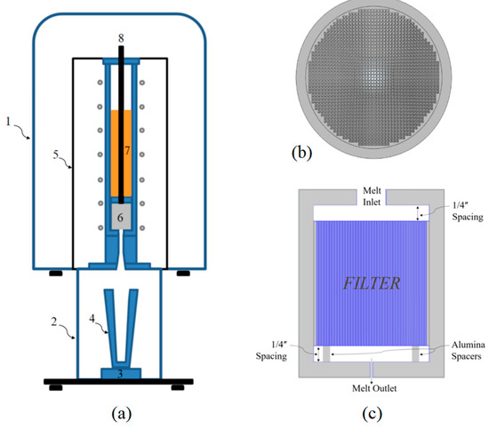
Figure 1.
The schematic views of the experimental setup, adapted from references [10,13,15]: (a) The experimental apparatus: (1) Furnace Dome, (2) Lower Chamber, (3) Load Cell, (4) Metallic Mold, (5) Furnace setup, (6) Alumina Filter, (7) Steel Melt, (8) Alumina Stopper Rod, (b) the cemented monolithic filter used in the experiment, and (c) the filter setup.
A steel charge containing 0.012% C, 0.04 Ni, and 12–20% ppm of oxygen was heated to 1600 ± 10 °C in an argon-filled furnace dome. After the charge was melted, the initial desired oxygen content was increased to 400–500 ppm by the addition of reagent-grade Fe2O3 powder to the charge. Then, it was maintained for 30 min to homogenize the melt. Later, a sample was taken from the center of the melt, and a known amount of high-purity aluminum wire was added to the melt. After 3 min, a sample from the center of the melt was taken to obtain the content of the alumina before filtration. Then, the top chamber was pressurized with argon. The alumina stopper rod was removed to let the molten steel flow through the filter setup. The filtered steel was then casted in a metallic mold that was placed in the lower chamber of the apparatus. In the investigations of the abovementioned studies, the concentration of alumina inclusions in the unfiltered and filtered steel melts were obtained and compared. Meanwhile, the effects of the square-celled monolithic alumina filter height, as well as steel flow rate on the concentration of alumina inclusions in the filtered melts, were also studied.
3. Methodology
3.1. Mathematical Modeling Modeling
To evaluate particle entrapment using CFD and to compare the results to the previous experimental findings, a three-dimensional model representing the experimental filtration setup was created. The model simulates a perfectly sealed filter where no gap exists between the filter holder and the filter media. Recently, it was shown that the filters need to be properly sealed to prevent fluid bypassing [37]. In addition, to avoid simulation and convergence complications, it was also assumed that the filter is made as part of the alumina crucible. Therefore, the alumina spacers shown in Figure 1c were neglected in the CFD model. The model was created according to the actual filter setup and experimental apparatus dimensions, as shown in Figure 1 and Table 1 and as explained elsewhere [10,13,15]. In addition, the filter matrix; particle and fluid properties, e.g., particle density, fluid density, and fluid temperature; and dynamic viscosity were set according to the experimental conditions presented in Table 2 and explained elsewhere [10,13,15,38].

Table 1.
Filter setup dimensions [10,13,15].
Table 2.
Steel and Alumina Inclusion properties.
To decide upon the fluid flow regime and to choose an appropriate module in the software, the Reynolds numbers were calculated. The Reynolds number for the overall flow (Re) and the particle relative Reynolds number () can be calculated as follows [39,40,41,42,43,44]:
where (kg/m3) is the fluid density, u (m/s) is the fluid velocity, l (m) is the characteristic length, µ (Pa·s) is the fluid dynamic viscosity, v (m/s) is the particle velocity, and dp (m) is the particle diameter. In a pipe-like configuration, the characteristic length l (m) could be replaced with hydraulic diameter (m).
S. Ali et al. measured and reported the interstitial velocity for the various experimental trials. In addition, their experiments included alumina inclusion sizes from 1 to 5 µm. In this research, the experimental condition correlating to the interstitial velocity 0.08 cm/s for a 5 cm-long monolithic alumina filter with a filter porosity ε equal to 0.63 was analytically obtained. Meanwhile, particle trajectories of the alumina inclusions larger than 5 µm and up to 100 µm were also simulated.
In an incompressible flow where the density is constant, one may use the continuity Equation (3) [43]. Here, when the interstitial velocity, porosity, inlet, and outlet diameters, as well as number of the pores and pore dimensions, are known, one may calculate the flow rates at the inlet, the spacer between the inlet and filter pores, the spacer between the filter pores and outlet, and lastly, the outlet. The calculated values were 1.33, 0.07, 0.07, and 214.2 cm/s, respectively.
Table 3 presents the calculated particle relative Reynolds numbers. Here, the maximum possible velocity difference was used in calculations to obtain the highest Reynolds number, i.e., the velocity difference equals the fluid velocity. The obtained numbers are needed to navigate in selecting adequate forces for calculating particle trajectories. The fluid flow Reynolds numbers at the inlet, filter pore, and outlet were found to be ~226, 1.2, 502 and 2865 respectively. The flow regime at Re < 2300 [39,41,43] is considered to be laminar. As a result, in all sections the Reynolds number is less than 2300, except for the outlet. However, the outlet is at the downstream. Therefore, the laminar flow could be applied to the whole domains of the system. As a result, a 2-step simulation to solve the relevant physics was used [42]. The first step calculates the steady flow fields through the modeled filter setup. The second step is to calculate the transport of the solid particles using an unsteady solver based on the results obtained from the first step, i.e., the steady flow filed calculations or unidirectional/one-way coupling [42]. For that reason, the “Laminar Flow” and the “Particle Tracing for Fluid Flow” modules in COMSOL Multiphysics® 6.0 software were used. Consequently, the following governing transport equations need to be solved:
Table 3.
Calculated Particle Relative Reynolds numbers.
- 1.
- The Navier–Stokes equations for incompressible fluids, containing continuity and conservation of momentum.
- 2.
- The Newton’s second law for the motion of particles in the fluid flow.
To compensate for time and calculation memory costs, only one-quarter of the filter setup was simulated, as shown in Figure 2. An inlet and a spacing section were connected to the top of the filter. Then, the lower part of the filter was connected to a spacing section and an outlet. Therefore, the simulated fluid entered the inlet, flowed through the spacer and filter pores, and exited the filter, lower spacer, and outlet from the opposite side, as indicated elsewhere [10,13,15].
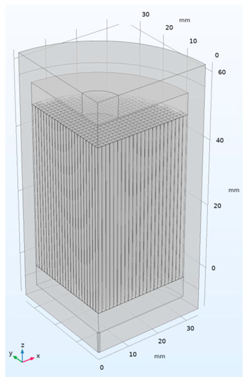
Figure 2.
A three-dimensional (3D) view of a quarter of the modeled filter setup.
3.2. Assumptions
The following assumptions were made to perform the mathematical modeling of the fluid flow and particle tracing in the fluid flow:
- Fluid Flow Simulations
- The fluid, filter, and particle properties were identical in all quarters of the whole filter setup.
- No fluid bypassing was considered. The filter was made as part of the alumina crucible.
- Temperature was assumed to be constant.
- The solution was independent of time, i.e., a steady-state solution.
- The gravitational force was considered.
- Incompressible Newtonian fluid with a constant fluid density and viscosity was considered.
- No heat transfer to/from the ambient medium was considered.
- There was no fluid–wall interaction.
- The walls were assumed to be straight and smooth using a no-slip boundary condition.
- Particle Tracing in Fluid Flow
- The fluid, filter, and particle properties were identical in all quarters of the whole filter setup.
- Fluid–particle interaction was not considered (unidirectional or one-way coupling).
- Particle–particle interaction was not considered.
- The particles were assumed to be spherical, following the findings of reference [13].
- Particles did not displace the fluid they occupied.
- Properties of the steel containing 0.012 pct. C, 0.04 Ni were assumed to be the same as iron at 1873 (K).
3.3. The Transport Equations
In an incompressible, isothermal Newtonian flow, i.e., where density and viscosity are constant, the steady-state fluid flow is described by the Navier–Stokes equations. The Navier–Stokes equations, including the continuity and momentum equations, can be written as follows [41]:
where (kg/m3) is the fluid density, u (m/s) is the velocity vector of the fluid, T (K) is the absolute temperature, p (Pa) is the pressure of the fluid, I (unitless) is the identity matrix, µ (Pa.s) is the dynamic viscosity of the fluid, and F (N/m3) is the volume force vector.
When immersed in a fluid flow, any body of any shape will experience forces from the fluid flow [43]. The motion of the particles in a fluid flow can be described with Newton’s second law [42,45]:
where mp (kg) is the particle mass, v (m/s) is the velocity of the particle, Ft (N) is the total force exerted on the particle, and q (m) is the particle position. Here, as presented in Equation (6), the total force may include gravitational Fg, drag FD, virtual mass FVM, pressure gradient FP, lift FL, and Brownian FB forces [42].
The gravitational force is calculated using Equation (7). Since the fluid density is also considered, the equation also contains the buoyancy force [42].
where g (m/s2) is the acceleration of gravity, which is equal to ~9.8, and (kg/m3) is the particle density.
The drag force acts in the direction opposite of the relative velocity of the particle with respect to the fluid [42]. Drag is essentially a flow loss [43]. The drag force is calculated using Stokes’ drag law, as shown in Equation (8). However, the Stokes drag is applicable for particles travelling through creeping flow, i.e., a fluid flow with a very low Reynolds number: 0 ˂ Re ˂ 1 [40,42,43,46]. In the current study, the fluid in the pores flowed at a low velocity, 0.08 (cm/s), with the calculated Reynolds number close to 1.2. Meanwhile, for all particles in this study, the particle relative Reynolds number was less than one in most sections of the filter setup, as seen in Table 3. On the other hand, in the rest of the domains, the relative Reynolds number was not less than one and varied with particle size, as presented in Table 3. In such cases, the standard drag correlation that adjusts the drag force based on the relative Reynolds number could be used. The standard drag correlation, i.e., the modified Stokes drag force, was calculated according to Stokes’ drag law and by applying Equations (8)–(12) [40,42,45]:
where τp (s) is the particle velocity response times, CD is a dimensionless drag coefficient, and w = log Rer.
The virtual mass and pressure gradient forces are most significant when the density of the particle is similar or less than the fluid density [42,47,48]. The virtual mass represents the acceleration of the fluid as it occupies the empty space that a moving particle leaves behind, resulting in a virtual increase in particle mass [42,47]. As shown in Table 2, fluid density is larger than particle density. The virtual increase of the particle mass, i.e., the part of the fluid with higher density, needs to be accelerated up to the particle velocity, which, on the other hand, requires an increase in the pressure gradient to accelerate the whole mixture [47]. The virtual mass and pressure gradient terms could be calculated using Equations (13)–(15) [42,48]:
where mf (kg) is the mass of the fluid displaced by the particle volume, and the material derivative D corresponds to the fluid velocity direction.
In a non-uniform velocity field, particles are also subject to lift force [42,43,46]. The lift force acts along the direction of the gradient of the fluid velocity, i.e., perpendicular to the flow direction [42,43,46]. In Comsol Multiphysics 6.0, the Saffman (FLS) and the wall-induced (FLW) lift forces are available [42]. The Saffman lift force is applicable for particles far from the walls. The wall-induced lift force is a specialized formulation that accounts for the effects of the nearby walls as particles travel through the channels [42]. Therefore, the wall-induced drag force was applied to the filter pores, i.e., channels, and the Saffman drag force was used for the remaining domains. The Saffman and wall-induced drag forces can be calculated as follows [42,46,49]:
where rp (m) is the particle radius, Lv (m/s) is the relative velocity, D (m) is the distance between the channel walls, s is the non-dimensionalized distance from the particle to the reference wall divided by D, and G1 and G2 are functions of non-dimensionalized wall distances and n is the wall normal at the nearest point on the reference wall.
The Brownian force FB was ignored for particles larger than one micron as it is believed to be significant only for submicron particles [45,50].
3.4. Boundary Conditions
The complete list of the boundary conditions for fluid flow and particle tracing studies in the system is given in Table 4. In fluid flow studies, a uniform velocity of 1.33 (cm.s−1) at the inlet was selected, no slip conditions were set for the inner walls, and and symmetry conditions for the cut plane walls were considered. In single-phase fluid flow in Comsol Mutliphysics 6.0, a no-slip wall is a wall where the fluid velocity relative to the wall velocity is zero, and the symmetry boundary condition stipulates no penetration and vanishing shear stress [41]. At the outlet, zero pressure and no viscous stress were assumed. In the fluid flow simulation, in addition to the pressure p, the velocity field components u in the x, y, and z directions were calculated throughout the geometry according to the transport Equations (4) and (5).
Table 4.
Boundary conditions.
In particle tracing studies, particles are released at time zero at the inlet. Here, the initial position of the particles was selected to be random, and the initial velocity was set according to the velocity of the fluid at that position. The particles were allowed to stick to the interior walls as soon as they hit the walls. It is believed [10,13] that alumina inclusion removal in molten steel consists of two steps: (1) first transport of inclusions by the molten fluid to the walls of the filter, and (2) the sintering of the inclusions to the filter surface and filter walls due to the high temperature and high interfacial energy of alumina inclusions in molten steel to each other and to the refractory walls [10,13,25].
In particle tracing for the fluid flow module, whenever a particle reached the symmetry wall, it left the model. However, from the same position, a same-size particle with an incoming velocity that mirrors the outgoing velocity entered the model, i.e., as if the particle had hit a wall with bounce condition [42]. At the outlet, particles were allowed to freeze once reaching the outlet wall. In particle tracing simulations the, particle position q and particle velocity v in the x, y, and z directions were calculated throughout the geometry according to the Newtonian formulation in Equation (6).
4. Results
4.1. Mesh Independence
To obtain the optimum mesh for the CFD modeling, several mesh options were configured, and the effects of mesh element sizes on mathematically obtained mass flow rates at a given outlet velocity were compared. A summary of the selected mesh parameters, including the selected mesh type, minimum and maximum element sizes in the domains and boundaries, the total mesh element, and calculation time, are presented in Table 5. The obtained estimated mass flow rates for each mesh option are illustrated in Figure 3. The CFD-estimated mass flow rate obtained with mesh option 7 provided the optimum mesh. At this point, the average mass flow rate did not improve with further mesh refinement, as shown in Figure 3. Therefore, the solution was considered to be independent of the mesh size. Thus, mesh option 7 was selected for the remaining mathematical modeling work.
Table 5.
Mesh independence study parameters.
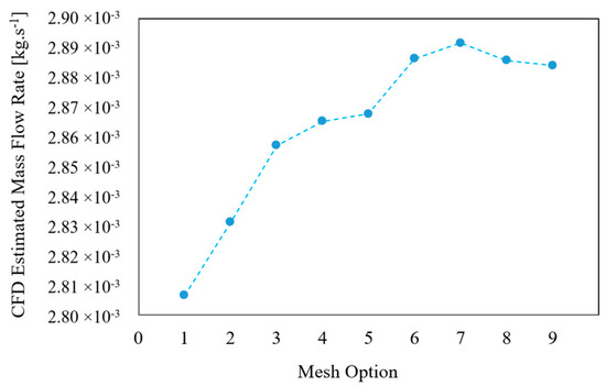
Figure 3.
Estimated mass flow rate as a function of the mesh option.
4.2. Fluid Flow Calculations
The mathematically obtained velocity magnitudes and velocity field streamlines through the modeled filter setup are illustrated in Figure 4a,b. As shown in the figures, higher-velocity magnitudes at the inlet and outlet sections as well as non-uniform velocity streamline in the regions before and after filter pores could be observed. On the other hand, there was a uniform low-velocity field in the filter pore channels. To be more specific, fluid entered the inlet with an initial velocity and continued to flow along a relatively straight streamline with a uniform velocity toward the end of the inlet. At this point, fluid freely expanded and spread in the space on the top of the filter, i.e., the spacer. Here, the streamline and velocity magnitude varied in different parts of the domain. This was due to a sudden change in the domain shape from the inlet to spacer, as well as fluid leaving the spacer to the pores. As shown in Figure 4a, higher-velocity magnitudes in the area closer to the inlet could be observed, while toward the ends of the spacer in the x-axis, the velocity was reduced. Furthermore, the fluid initially hit the region of the filter that was in front of the inlet. Then, the rest of the flow was carried out toward the edges while slowing down in momentum. Throughout the pores, the fluid flowed at a very slow rate and along a straight streamline toward the end of the pores, as presented in Figure 4b. Thereafter, the velocity magnitude gradually increased while the streamlines converge and the fluid flowed toward the outlet and left the domain.
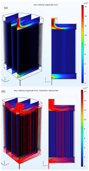
Figure 4.
CFD predicted steel flow properties in the filter setup: (a) Velocity magnitude, (b) Velocity streamline.
4.3. Particle Tracing in Fluid Flow
Particle trajectories of the 100, 70, 50, 30, 20, 10, 5, and 1 µm alumina inclusions were studied independently of each other. In each study, 100 particles were released at time zero from random initial positions at the inlet due to the fact that their distributions were reported to be non-uniform [13]. The particle trajectories were mathematically calculated using Equation (6). Meanwhile, the required preliminary data, e.g., the fluid density, the fluid viscosity, and velocity at each grid point, were provided by the initially solved fluid flow study step. Enough time was given until there were no active particles in the system, i.e., particles were either stuck in the filtration setup or had left the system from the outlet. The required time given to the unsteady particle tracing step was found by trial and error. The predicted particle removal rates, i.e., the percentage of the particles removed from the simulated molten steel by the simulated filtration setup, is illustrated in Figure 5 as a function of particle size. Figure 6 illustrates the position of the particles when there was no active particle in the system. It can be observed in the figures that 100% of the particles larger than 50 µm were captured by the filtration setup. Almost all 50 µm particles were also captured, but from this point, as the particle size decreased, the particle removal rate also declined. The non-captured particles traveled through the filter pores and channels and continued along the streamline toward the outlet.
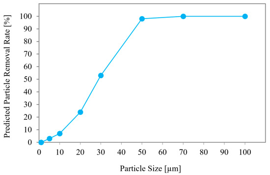
Figure 5.
Predicted particle removal rate as a function of particle size.
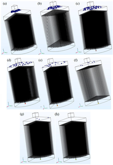
Figure 6.
Position of the removed particles: (a) 100 µm, (b) 70 µm, (c) 50 µm, (d) 30 µm, (e) 20 µm, (f) 10 µm, (g) 5 µm, and (h) 1 µm.
5. Discussions
The physical refining of a molten steel melt using a square-celled monolithic extruded alumina filter was simulated. Specifically, the laminar fluid flow of the steel melt was simulated, and particle trajectories of the alumina inclusions in the size range of 1–100 µm were numerically obtained. As illustrated in Figure 4, the fluid flow rates varied, and the fluid followed an alternating streamline due to the domain change in the sections of the modeled filter setup. Therefore, particles were exposed to different flow rates in different domains of the filter setup. In total, eight case studies were performed, and in each study, 100 particles were released at time zero from random initial positions at the inlet. As a result, the released particles in the inlet picked up the fluid velocity and initially followed the streamline. However, the particles, due to their size, behaved differently along the path in different parts of the setup.
In general, a filtration process could be categorized into surface and depth filtration [6,13,15,17,18,51,52,53,54]. In surface filtration, particles are either removed due to their larger size compared to the filter pores and openings, also known as sieving [6,17,52,53], and/or by clustering of the particles and net formation, i.e., cake filtration, on the top of the filter openings [6,13,17,18,52,53]. In this region, particles tend to collide and bond. This forms a net of particles that acts as an additional filter, which results in the removal of more particles. On the other hand, particles that are not captured by sieving nor by cake filtration, i.e., small size particles, enter the filter pores. Here, depending on the fluid velocity and the type of filter or the path ahead, the particles are either captured in the filter through depth filtration [6,13,17,18,52,53] or follow the streamline and leave the filter. An effective depth filtration is believed to happen mainly in aggregates or granular beds, as well as foam filters, due to the tortuous path the fluid and particles have to flow [6,52,53]. Here, the torturous internal pore surface area provides higher probabilities of capturing and retaining particles from a molten metal [17,51,53].
It is believed [10,13,15,17,18] that the particles which enter the pores are mainly captured in the upper section of the filter and close to the filter openings at the entrance. As explained earlier, due to clustering and agglomeration of the inclusions, i.e., net or cake formation, the fluid would be forced to flow only through the free path available. As a result, at the entrance in the top of the filter, the fluid flow streamline would locally experience irregularities and would not be able to follow the streamline in the same manner as CFD predicted in Figure 4. Such streamline irregularities would bring the particles close to the surface of the alumina filter [6,10,13]. Moreover, it is known that the molten steel does not wet alumina particles. In addition, the dispersed particles in a non-wetting melt tend to reduce the surface tension by transferring themselves to a more stable state with a lower surface energy [6,10,13]. Consequently, a combination of the abovementioned factors would promote particle impaction to the walls of the filter when inclusions are in close vicinity of the filter surface [6,10,13,53,54]. Here, alumina inclusions sinter rapidly to the alumina surface of the filter medium [6,10,13,53,54]. As the flow passes this region, the fluid flow would return to its original rather straight streamline. Thus, the remaining small particles would mainly flow the streamline toward the filter exit and the outlet. Therefore, less depth filtration occurs [10,13,17] as the particles travel toward the exit of the filter.
In this study, it was shown that the mathematical modeling of particle collisions that result in clustering and agglomerations leading to the net formation, i.e., cake formation on the filter, is not yet possible in COMSOL Multiphysics. Thus, such particle–particle interactions were not considered. In addition, fluid–particle interaction was not included in the model. Therefore, the particle tracing was a one-way coupling study, i.e., only the fluid affected the particle motion, not vice versa. Regardless of the simulation limitations, the position of the removed particles and the numerically obtained particle removal rate for each particle size are presented in Figure 5 and Figure 6. It can be observed that 100% of the particles larger than 50 µm were captured in the region between the inlet and filter. The particles had about half the density of the molten steel and were rather large to follow the streamline toward the filter openings at such low flow rates. Here, due to the density/buoyancy effect, they floated and hit the alumina wall on the top of the filter. Almost all 50 µm particles were also captured in the same way as larger particles, but from this point, as the particle size decreased, less particles were captured due to buoyancy. The non-captured particles entered the filter pores and continued the streamline toward the outlet. It is still a difficult task to create a mathematical model considering particle clustering and agglomeration which results in net or cake formation. Therefore, the depth filtration could not be predicted. In order to make a more reliable prediction, the mathematical model needs to be continuously developed to include more complex physical phenomena.
6. Conclusions
A computational fluid dynamics study, including simulations of both fluid flow and particle tracing of non-metallic alumina inclusions, in the size range of 1–100 µm, was conducted from a steel melt through a square-celled monolithic alumina filter. The CFD study was performed in two steps. First, the steady-state laminar fluid flow, i.e., molten steel at 1600 °C, was simulated. The solution was calibrated to be independent of the mesh size. Then, particle trajectories were predicted using an unsteady solver based on the results obtained from the first step. Recirculation of the flow in the spacer in the upper section of the filtration setup and/or on the top of the filter led to the removal of large particles from the fluid flow. The smaller particles, however, followed the streamline along the filter channels and left the simulated filtration setup from the outlet. The predicted results for particles in the size range of ≤5 µm were compared to the published experimental data. The main conclusions of the study can be summarized as follows:
- The modeled filtration setup could capture 100% of the particles larger than 50 µm.
- The percentage of the filtered particles decreased from 98% to 0% in the particle size range from 50 µm to 1 µm.
- The current model has a limitation in predicting particle filtration for particles in the size range of ≤5 µm.
- Further modeling development of physical filtration is required to include particle clustering and agglomeration which results in net or cake formation.
Author Contributions
Conceptualization, S.A.; Methodology, S.A.; Software, S.A.; Validation, S.A.; Formal analysis, S.A.; Investigation, S.A.; Resources, S.A. and P.G.J.; Data curation, S.A.; Writing—original draft, S.A.; Writing—review and editing, S.A., D.-Y.S. and P.G.J.; Visualization, S.A.; Supervision, D.-Y.S. and P.G.J.; Project administration, S.A. All authors have read and agreed to the published version of the manuscript.
Funding
This research received no external funding.
Data Availability Statement
All data is available in the article.
Conflicts of Interest
The authors declare no conflict of interest.
References
- Leonov, A.N.; Dechko, M.M. Theory of Design of Foam Ceramic Filters for Cleaning Molten Metals. Refract. Ind. Ceram. 1999, 40, 537. [Google Scholar] [CrossRef]
- Aneziris, C.G.; Dudczig, S.; Emmel, M.; Berek, H.; Schmidt, G.; Hubalkova, J. Reactive Ffilters for Steel Melt Filtration. Adv. Eng. Mater. 2013, 15, 46. [Google Scholar] [CrossRef]
- Akbarnejad, S.; Jonsson, L.; Kennedy, M.W.; Aune, R.E.; Jönsson, P. Analysis on Experimental Investigation and Mathematical Modeling of Incompressible Flow through Ceramic Foam Filter. Metall. Mater. Trans. B 2016, 47, 2229. [Google Scholar] [CrossRef]
- Yang, Y.; Maeda, Y.; Takita, M.; Nomura, H. Effect of Flow Behavior on the Removal of Inclusions by Filter. Int. J. Cast Metals Res. 1997, 10, 165. [Google Scholar] [CrossRef]
- Atkinson, H.V.; Shi, G. Characterization of Inclusions in Clean Steels: A Review Including the Statistics of Extremes Methods. Prog. Mater. Sci. 2003, 48, 457. [Google Scholar] [CrossRef]
- Smothers, W.J. Application of Refractories: Ceramic Engineering and Science Proceedings; The American Ceramic Society, Inc.: Columbus, OH, USA, 1987; Volume 8, p. 107. [Google Scholar]
- Zhang, L.; Thomas, B.G. State of the Art in Evaluation and Control of Steel Cleanliness. ISIJ Int. 2003, 43, 271. [Google Scholar] [CrossRef]
- Zhang, L.; Thomas, B.G. Inclusions in Continuous Casting of Steel. In Proceedings of the XXIV National Steelmaking Symposium, Morelia, Mexico, 26–28 November 2003; p. 138. [Google Scholar]
- Silva, A.L.V.d.C. Non-metallic Inclusions in Steels–Origin and Control. Mater. Res. Tech. 2018, 7, 283. [Google Scholar]
- Apelian, D.; Mutharasan, R.; Ali, S. Removal of Inclusions from Steel Melts by Filtration. Mater. Sci. 1985, 20, 3501. [Google Scholar] [CrossRef]
- Wang, Y.; Karasev, A.; Jönsson, P.G. Comparison of Nonmetallic Inclusion Characteristics in Metal Samples Using 2D and 3D Methods. Steel Res. Int. 2020, 91, 1900669. [Google Scholar] [CrossRef]
- Fan, X.; Zhang, L.; Ren, Y.; Yang, W.; Wu, S. Metals, The Effect of Aluminum Addition on the Evolution of Inclusions in an Aluminum-Killed Calcium-Treated Steel. Metals 2022, 12, 181. [Google Scholar] [CrossRef]
- Ali, S.; Mutharasan, R.; Apelian, D. Physical Refining of Steel Melts by Filtration. Metall. Mater. Trans. B 1985, 16, 725. [Google Scholar] [CrossRef]
- Dippenaar, R Industrial Uses of Slag (the Use and Re-use of Iron and Steelmaking Slags). Ironmak. Steelmak. 2005, 32, 35. [CrossRef]
- Ali, S.; Apelian, D.; Mutharasant, R. Refining of Aluminum and Steel Melts by the Use of Multi-Cellular Extruded Ceramic Filters. Canad. Metall. Q. 1985, 24, 311. [Google Scholar] [CrossRef]
- Uemura, K.; Takahashi, M.; Koyama, S.; Nitta, M. Filtration Mechamism of Non-metallic Inclusions in Steel by Ceramic Loop Filter. ISIJ Int. 1992, 32, 150. [Google Scholar] [CrossRef]
- Scheffler, M.; Colombo, P. Cellular Ceramics: Structure, Manufacturing, Properties and Applications; Wiley-VCH Verlag GmbH & Co. KGaA: Weinheim, Germany, 2005; p. 621. [Google Scholar]
- Damoah, L.N.W.; Zhang, L. Removal of Inclusions from Aluminum through Filtration. Metall. Mater. Trans. B 2010, 41, 886. [Google Scholar] [CrossRef]
- Kennedy, M.W.; Akhtar, S.; Bakken, J.A.; Aune, R.E. Electromagnetically Modified Filtration of Aluminum Melts—Part I: Electromagnetic Theory and 30 PPI Ceramic Foam Filter Experimental Results. Metall. Mater. Trans. B 2013, 44, 691. [Google Scholar] [CrossRef]
- Sahai, Y. Tundish Technology for Casting Clean Steel: A Review. Metall. Mater. Trans. B 2016, 47, 2095. [Google Scholar] [CrossRef]
- Ånmark, N.; Karasev, A.; Jönsson, P.G. The Effect of Different Non-Metallic Inclusions on the Machinability of Steels. Materials 2015, 8, 751. [Google Scholar] [CrossRef]
- Braun, T.B.; Elliott, J.F.; Flemings, M.C. The Clustering of Alumina Inclusions. Metall. Mater. Trans. B 1979, 10, 171. [Google Scholar] [CrossRef]
- McLean, A.; Ward, R.G.; Strathdee, B. Aluminum Deoxidation Products in Rimmed Steel. JOM 1965, 17, 526. [Google Scholar] [CrossRef]
- Wang, Y.; Karasev, A.; Jönsson, P.G. Non-metallic Inclusions in Different Ferroalloys and Their Effect on the Steel Quality: A Review. Metall. Mater. Trans. B 2021, 52, 2892. [Google Scholar] [CrossRef]
- Singh, S.N. Mechanism of Alumina Buildup in Tundish Nozzles During Continuous Casting of Aluminum-Killed Steels. Metall. Mater. Trans. B 1974, 5, 2165. [Google Scholar] [CrossRef]
- Debroy, T.; Sychterz, J.A. Numerical Calculation of Fluid Flow in a Continuous Casting Tundish. Metall. Mater. Trans. B 1985, 16, 497. [Google Scholar] [CrossRef]
- Zhang, L.; Pluschkell, W. Nucleation and Growth Kinetics of Inclusions during Liquid Steel Deoxidation. Ironmak. Steelmak. 2003, 30, 106. [Google Scholar] [CrossRef]
- Yin, H.B.; Shibata, H.; Emi, T.; Suzuki, M. “In-situ” Observation of Collision, Agglomeration and Cluster Formation of Alumina Inclusion Particles on Steel Melts. ISIJ Int. 1997, 37, 936. [Google Scholar] [CrossRef]
- Ende, M.A.V. Formation and Morphology of non-Metallic Inclusions in Aluminium Killed Steels. Ph.D. Thesis, Katholieke Universiteit, Leuven, Belgium, 2010. [Google Scholar]
- Lee, W.; Kim, J.G.; Jung, J., II; Huh, K.Y. Prediction of Nozzle Clogging through Fluid–Structure Interaction in the Continuous Steel Casting Process. Steel Res. Int. 2021, 92, 2000549. [Google Scholar] [CrossRef]
- Michelic, S.K.; Bernhard, C. Significance of Nonmetallic Inclusions for the Clogging Phenomenon in Continuous Casting of Steel––A Review. Steel Res. Int. 2022, 93, 2200086. [Google Scholar] [CrossRef]
- Wang, J.; Xia, M.; Wu, J.; Ge, C. Ladle Nozzle Clogging in Vacuum Induction Melting Gas Atomization: Influence of the Melt Viscosity. Metall. Mater. Trans. B 2022, 53, 2386. [Google Scholar] [CrossRef]
- Liang, W.; Li, J.; Lu, B.; Zhi, J.G.; Zhang, S.; Liu, Y. Analysis on Clogging of Submerged Entry Nozzle in Continuous Casting of High Strength Steel with Rare Earth. Iron and Steel Res. Int. 2022, 29, 34. [Google Scholar] [CrossRef]
- Bulkowski, L.; Galisz, U.; Kania, H.; Kudliński, Z.; Pieprzyca, J.; Barański, J. Industrial Tests of Steel Filtering Process. Arch. Metall. Mater. 2012, 57, 363. [Google Scholar] [CrossRef]
- Chakraborty, S.; Malley, R.J.O.; Bartlett, L.; Xu, M. Efficiency of Solid Inclusion Removal from the Steel Melt by Ceramic Foam Filter: Design and Experimental Validation. In Proceedings of the 122nd Metalcasting Congress, Forth Worth, TX, USA, 3–5 April 2018. [Google Scholar]
- Chakraborty, S. Removal of Non-metallic Inclusions from Molten Steel by Ceramic Foam Filtration. Ph.D. Thesis, Missouri University of Science and Technology, Rolla, MO, USA, 2020. [Google Scholar]
- Akbarnejad, S.; Pour, M.S.; Jonsson, L.T.I.; Jonsson, P.G. Effect of Fluid Bypassing on the Experimentally Obtained Darcy and Non-Darcy Permeability Parameters of Ceramic Foam Filters. Metall. Mater. Trans. B 2017, 48, 197. [Google Scholar] [CrossRef]
- Assael, M.J.; Kakosimos, K.; Banish, R.M.; Brillo, J.; Egry, I.; Brooks, R.; Quested, P.N.; Mills, K.C.; Nagashima, A.; Sato, Y.; et al. Reference Data for the Density and Viscosity of Liquid Aluminum and Liquid Iron. Phys. Chem. Ref. Data 2006, 35, 285. [Google Scholar] [CrossRef]
- Fox, R.W.; McDonald, A.T.; Pritchard, P.J. Introduction to Fluid Mechanics; John Wiley & Sons Inc.: Hoboken, NJ, USA, 2004. [Google Scholar]
- Johnson, R.W. The Handbook of Fluid Dynamics; CRC Press: Boca Raton, FL, USA; Springer: Berlin/Heidelberg, Germany, 1998. [Google Scholar]
- FD Module User’s Guide, COMSOL Multiphysics Version 6.0; Comsol: Stockholm, Sweden, 2021.
- Particle Tracing Module User’s Guide, COMSOL Multiphysics Version 6.0; Comsol: Stockholm, Sweden, 2021.
- White, F.M. Fluid Mechanics; McGraw-Hill: New York, NY, USA, 2010. [Google Scholar]
- Haider, A.; Levenspiel, O. Drag Coefficient and Terminal Velocity of Spherical and Nonspherical Particles. Powder Technol. 1989, 58, 63. [Google Scholar] [CrossRef]
- Introduction to Particle Tracing Module, COMSOL Multiphysics Version 6.0; Comsol: Stockholm, Sweden, 2021.
- Saffman, P.G. The lift on a Small Sphere in a Slow Shear Flow. Fluid Mech. 1965, 22, 385. [Google Scholar] [CrossRef]
- Paladino, E.E.; Maliska, C.R. Virtual mass in accelerated bubbly flows. In Proceedings of the 4th European Thermal Sciences, National Exhibition Centre, Birmingham, UK, 29–31 March 2004. [Google Scholar]
- Maxey, M.R.; Riley, J.J. Equation of Motion for a Small Rigid Sphere in a Nonuniform Flow. Phys. Fluids 1983, 26, 883. [Google Scholar] [CrossRef]
- Ho, B.P.; Leal, L.G. Inertial Migration of Rigid Spheres in Two-dimensional Unidirectional Flows. Fluid Mech. 1974, 65, 365. [Google Scholar] [CrossRef]
- Li, A.; Ahmadi, G. Dispersion and Deposition of Spherical Particles from Point Sources in a Turbulent Channel Flow. Aero. Sci. Technol. 1992, 16, 209. [Google Scholar] [CrossRef]
- Apelian, D.; Mutharasan, R. Filtration: A Melt Refining Method. JOM 1980, 32, 14. [Google Scholar] [CrossRef]
- Raiber, K.; Hammerschmid, P.; Janke, D. Experimental Studies on Al2O3 Inclusion Removal from Steel Melts Using Ceramic Filters. ISIJ Int. 1995, 35, 380. [Google Scholar] [CrossRef]
- Gauckler, L.J.; Waeber, M.M.; Conti, C.; Jacob-Duliere, M. Ceramic Foam for Molten metal Filtration. JOM 1985, 37, 47. [Google Scholar] [CrossRef]
- Apelian, D.; Sutton, W.H. Utilization of Ceramic Filters to Produce Cleaner Superalloy Melts. In Proceedings of the 5th International Symposium on Superalloys, Champion, PA, USA, 7–11 October 1984; p. 421. [Google Scholar]
Disclaimer/Publisher’s Note: The statements, opinions and data contained in all publications are solely those of the individual author(s) and contributor(s) and not of MDPI and/or the editor(s). MDPI and/or the editor(s) disclaim responsibility for any injury to people or property resulting from any ideas, methods, instructions or products referred to in the content. |
© 2023 by the authors. Licensee MDPI, Basel, Switzerland. This article is an open access article distributed under the terms and conditions of the Creative Commons Attribution (CC BY) license (https://creativecommons.org/licenses/by/4.0/).