Abstract
Texture analysis is key to better understanding of the relationships between the microstructures of the materials and their properties, as well as the use of models in process systems using raw signals or images as input. Recently, new methods based on transfer learning with deep neural networks have become established as highly competitive approaches to classical texture analysis. In this study, three traditional approaches, based on the use of grey level co-occurrence matrices, local binary patterns and textons are compared with five transfer learning approaches, based on the use of AlexNet, VGG19, ResNet50, GoogLeNet and MobileNetV2. This is done based on two simulated and one real-world case study. In the simulated case studies, material microstructures were simulated with Voronoi graphic representations and in the real-world case study, the appearance of ultrahigh carbon steel is cast as a textural pattern recognition pattern. The ability of random forest models, as well as the convolutional neural networks themselves, to discriminate between different textures with the image features as input was used as the basis for comparison. The texton algorithm performed better than the LBP and GLCM algorithms and similar to the deep learning approaches when these were used directly, without any retraining. Partial or full retraining of the convolutional neural networks yielded considerably better results, with GoogLeNet and MobileNetV2 yielding the best results.
1. Introduction
Texture analysis in images is important in a wide range of industries. It is not precisely defined, since image texture is not precisely defined, but intuitively, image texture analysis attempts to quantify qualities such as roughness, smoothness, heterogeneity, regularity, etc., as a function of the spatial variation in pixel intensities.
In materials, image texture analysis can be used to derive quantitative descriptors of the distributions of the orientations and sizes of grains in polycrystalline materials. Almost all engineering materials have texture, which is strongly correlated with their properties, such as mechanical strength, resistance to stress corrosion cracking and radiation damage, etc. In this sense, image textures and textures in materials are closely related.
In the case of metalliferous ores or rocks, image texture provides critical information with regard to the response of the materials during mining and mineral processing [1,2]. For example, more energy is generally required to liberate finely disseminated minerals from ores, i.e., ores with fine textures, than is the case with ores with coarse textures.
Characterization of the textural characteristics of materials, whether related to the microstructures of metals, mineral ores or the surface properties of materials, requires steps beyond simple qualitative descriptions of material textures to quantitative descriptions that can be used in models that can predict the behavior of the metals or ores in a given process or system [2].
A variety of such methods to quantify the textural appearance of materials has been proposed, as discussed comprehensively in a recent review by Ghalati et al. [3]. This includes a review of traditional approaches, as well as more recent approaches based on the use of learned features, as opposed to engineered features.
Few studies have been reported where some comparative assessment of methods was made. For example, Kerut et al. [4] reviewed quantitative texture analysis applied to the images generated by echocardiography. These were categorized as statistical methods, fractal methods, frequency domain methods and methods based on the use of wavelets. The latter was still an emerging approach but was considered to be a state-of-the-art method at the time, with 2D Haar dyadic wavelets recommended in particular.
In mineral processing, Kistner et al. [5] considered the application of grey level co-occurrence methods, local binary patterns, wavelets, steerable pyramids and textons and found that the latter approach was best able to capture patterns associated with flotation froth images, particulate solids and slurry flows.
More recently, transfer learning by use of convolutional neural networks has emerged as a strong contender as a state-of-the-art method in texture analysis [6]. Fu and Aldrich [7] found that AlexNet provides better flotation froth descriptors than methods based on the use of grey level co-occurrence matrices, wavelets and local binary patterns. Authors, such as Mormont et al. [8] and Xiao et al. [9], have conducted texture analysis with transfer learning methods. Mormont et al. [8] found that DenseNet and ResNet marginally yielded the best features for classification of histological images. Xiao et al. [9] concluded that transfer learning methods outperformed traditional methods, with InceptionV3 performing the best overall.
While these studies serve as a guide to the comparative merits of different texture analytical methods, the relative merits of different approaches are still not well documented in the literature. This study reviews developments in quantitative image texture analysis, and assesses the feasibility of state-of-the-art methods, with a focus on textures associated with material processing. This includes an assessment of different variants of transfer learning, based on zero, partial and full retraining of the feature layers of convolutional neural networks.
In the following section, image texture analysis in metal processing is briefly reviewed. This is followed by an explanation of the analytical methodology of the study. In Section 4, Section 5 and Section 6, the methodology is applied to case studies and in Section 7 and Section 8, the results are discussed, and the conclusions of the study are summarized.
2. Application of Texture Analysis in Metallurgical Engineering
2.1. Geometallurgical Models
Quantitative analysis of ore textures has seen exponential growth in the wake of recent developments in modern analytical instrumentation, such as the quantitative evaluation of minerals by Mineral Liberation Analyzer (MLA) [10,11,12], scanning electron microscopy (QEMSCAN) [10,13,14], and X-ray computer tomography [2,15]. These techniques are used to analyze ore textures on a microscale, with the ultimate goal to use this information in geometallurgical models that can be used to predict the performance of downstream process systems [11,16].
Textural descriptors recently considered include association indicator matrices [17], grey level co-occurrence matrices [18,19], continuous wavelet transforms [20,21] and local binary patterns [21], as well as descriptors obtained with convolutional neural networks [22]. These descriptors are not designed to identify the physical characteristics of the material directly, e.g., the grain size in polycrystalline materials. Instead, they indirectly represent such structures, considering that finer grain sizes would give rise to different textural appearances in images than coarser grain sizes would.
2.2. Microstructural Predictors of Metal Properties
Renzetti and Sortia [23] used grey level co-occurrence (GLCM) methods to characterize the microstructures in duplex stainless steels. Webel et al. [24] likewise made use of GLCM features to characterize the microstructures of low alloy steels. Velichko et al. [25] extracted morphological features from cast iron that could be used with support vector machines to classify cast iron microstructures. DeCost et al. [26] investigated the classification of the microstructures in a single ultrahigh carbon steel generated by different heat treatment conditions based on pixel-wise segmentation and fully connected neural networks. Azimi et al. [27] used deep neural networks to classify the microstructures of steel, specifically martensite, tempered martensite, bainite and pearlite. Gola et al. [28] made use of support vector machines using a combination of morphological parameters and textural features for classification of low carbon steels. Similarly, Beniwal et al. [29] proposed a general approach based on deep learning to predict material properties based on microstructural features.
2.3. Metal Surface Quality
Metal surface quality is an important element of the overall quality assessment of the production of metal components. As a consequence, the application of computer vision systems as a means to automate assessment continues to attract significant interest. Texture analysis in particular has recently been studied by a number of authors. For example, Trambitckii et al. [30] found a strong correlation between surface roughness and image features extracted with various algorithms.
Medeiros et al. [31] focused on the surface textures and appearance of corroded surfaces based on the evaluation of color and texture, with the latter represented by GLCM features. Guo et al. [32] showed that GLCM features can be used to classify defects in steel strip. Luo et al. [33] used local binary pattern (LBP) features to accomplish a similar objective on hot rolled steel strips.
Mao et al. [34] proposed a new algorithm, referred to as order-less scale invariant gradient local auto-correlation (OS-GLAC), for metal surface texture characterization. Their satisfactory results were even better when these features were combined with features obtained with a convolutional neural network. Luo et al. [33] made use of selectively dominant local binary patterns to detect surface defects in hot rolled steel strips.
2.4. Failure Analysis of Metals
Metal fractography is another area that can be cast as a problem in material texture analysis. For example, Das et al. [35] extracted GLCM features and ran length statistics from fractographs of 7075 Al alloys generated by impact tests under different processing conditions. These features were strongly correlated with the impact toughness of the alloys. Dutta et al. [36,37] used fractal analysis based on box counting, GLCM and run length statistics on fractographs of stainless steel for automatic characterization of fracture surfaces. The run length statistics yielded the best results in terms of accuracy and computational cost. Naik and Kiran [38] used LBPs to characterize and identify fracture in metals. Müller et al. [39] made use of GLCM for surface crack detection in fracture experiments. Bastidas-Rodriguez et al. [40] applied Haralick’s features (GLCM) texture energy laws and fractal dimension as descriptors to optical images of metals to discriminate between three different failure modes, using multilayer perceptrons and support vector machines. Dutta et al. [41] took a different approach based on geometric texture analysis. Using Voronoi tessellation on fractographs of 304LN stainless steel, they extracted four features, viz. Voronoi edges, mean area, mean elongation and mean perimeter of Voronoi polygons, which could, among other things, reliably predict the ductility of the steel.
The results from the literature indicate that a wide range of methods have been investigated for material texture analysis. GLCM methods appear to be the most popular, while deep learning approaches have only just started to emerge.
3. Analytical Methodology
Evaluation of the feature extraction algorithms was based on the following steps in each of three case studies, as schematically illustrated in Figure 1.
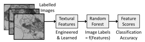
Figure 1.
Analytical methodology based on the extraction of features from labelled textural images of materials, followed by assessment of the ability of a random forest model to discriminate between textures using the features as the input.
- (a)
- Generation of two sets of textures A and B that were similar, but not identical. These textures were generated by Voronoi tessellation of random data with user-controlled parameters, and the diagrams were stored as JPG images.
- (b)
- Extraction of features from data textural image sets A and B with each of the algorithms, i.e., GLCM, LBP, textons, AlexNet, VGG19, ResNet50, GoogLeNet and MobileNetV2, described in more detail below.
- (c)
- Use of random forest models to discriminate between the textures using the GLCM, LBP, textons, AlexNet, VGG19, ResNet50, GoogLetNet and MobileNetV2 features as predictors. An exception was made with the trained convolutional neural networks, which were used end-to-end to classify the textures directly.
3.1. Grey Level Co-Occurrence Matrices
The grey level co-occurrence matrix, , of an image with parameters and , where is the distance between each pair of pixels in the image and is the number of grey levels considered in the image, as indicated in Figure 2.
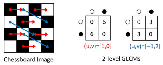
Figure 2.
A partial image of a chessboard (left) with binary co-occurrence matrices (right) showing the frequency of pairs of two grey levels (black and white), separated by a distance and direction, as specified by Cartesian coordinates (u,v).
Each entry , in the matrix denotes the number of times that a grey level is associated with a pair of pixels at displacement in the image.
The Haralick [42] set of image descriptors extracted from GLCM images is often used in image analysis. In this investigation, the following four features, namely energy (ENE), contrast (CON), correlation (COR) and homogeneity (HOM), were used.
In Equations (1)–(4), is the (i,j)th element of the normalized GLCM and and , and and are the means and standard deviations of matrix rows and columns.
The energy (ENE) is a measure of the local uniformity of the grey levels in the image. The contrast (CON) is a is a measure of the grey level variations between the reference pixels and their neighbors. The correlation (COR) is indicative of the linear dependency of grey levels in the GLCM. Homogeneity (HOM) is usually inversely related to the contrast and is an indication of the similarity of the off-diagonal elements in the GLCM is to the diagonal elements of the GLCM.
GLCM methods were some of the very first to be used in froth image analysis [43,44,45] and have since been considered extensively in a range of applications in mineral processing and material science.
3.2. Local Binary Patterns
Local binary patterns are generated from greyscale images by comparing the intensity of each pixel in the image to the intensities of pixels in its neighborhood [46]. The differences in the intensities between neighboring pixels () and center pixels () under consideration is set to either 0 or 1, by applying a binary thresholding function s:
Following that, the local binary pattern (LBP) is computed as shown in Equation (6), for all , 2 … P.
By applying the LBP operator in Equation (6) to each pixel in an image, as indicated in Figure 3, an image can be represented by an equisized 2D array of center pixel values and referred to as an LBP image. Counts of these values, as represented in an LBP histogram, serve as the features of the image.
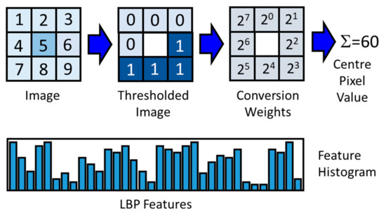
Figure 3.
Example of a center pixel (shaded), with its eight neighboring pixels (top, left), the values obtained through binary thresholding (top, middle) and the conversion weights by which the thresholded values are multiplied to give the decimal LBP value shown in place of the center pixel (top, right). A histogram of these values in the resulting LBP image is used as a basis for LBP features (bottom).
Variants of this approach are defined by the size of the pixel neighborhoods, the possible subdivision of the image in patches, as well as the inclusion of the number of transitions in the LBP vectors (uniformity) of the vectors. LBP feature extraction is a comparatively recent approach to multivariate image analysis in mineral processing [5,47,48,49,50].
3.3. Textons
Textons can be viewed as the centers of clusters of a localized filter response space that are generated through convolution of a training set of images with oriented spatial basis functions arranged in a filter bank [51], as indicated in Figure 4. Each pixel in an image is mapped to this feature space, while the cluster centers in the space are typically determined by k-means clustering. These cluster centers comprise what is referred to as a texton dictionary. A texton feature associated with an image consist of a count of the number of pixels assigned to the specific texton channel [5].
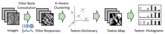
Figure 4.
Texton feature extraction from images based on filtering of images, extraction of localized filter vectors, clustering of the filter vectors in the vector feature space to construct a texton dictionary, mapping of the images to the dictionary and extracting the features as the resulting histogram counts.
In this investigation, the Schmid filter bank was used [52]. It consists of 13 rotationally invariant filters of the form described in Equation (7), where r represents the pixel coordinates in the image, s is the scale and t is the frequency or number of cycles in the Gaussian envelope of the filter [53].
To date, textons have not been widely used in image analysis in mineral processing, although some studies have indicated that it can provide superior models, when compared with more popular feature extraction algorithms, such as grey level co-occurrence matrix methods [5,49,54].
3.4. AlexNet
AlexNet is a deep neural network, developed by Alex Krizhevsky et al. [55] that won the ImageNet LSVRC-2010 competition in 2012 (https://www.image-net.org/challenges/LSVRC/index.php) (accessed date: 17 February 2022). It contains five convolution layers that operate with three-channel images of size 224 × 224 × 3 and uses 3 × 3 kernels for max pooling and either 11 × 11, 5 × 5 or 3 × 3 kernels for convolution.
3.5. VGG19
The VGG19 convolutional neural network was created by the Visual Geometry Group (VGG) at Oxford University and can be seen as a successor of AlexNet. It won the ImageNet competition in 2014. The VGG19 architecture made use of 3 × 3 kernels with a one-pixel stride and max pooling over a 2 × 2 window with a stride of two. In addition, the network made use of rectilinear (ReLU) units to introduce nonlinearity into the model and to improve computation during training.
3.6. ResNet50
ResNet50 is one of a number of variants of convolutional neural networks, such as ResNet18, ResNet101 and ResNet152. Despite being deeper than AlexNet and VGG19, it contains comparatively fewer parameters (weights), i.e., approximately 25.5 million. Unlike traditional, or shallow neural networks, such as one- or two-layer perceptrons, deep neural networks are prone to suffering from the so-called vanishing gradient problem. Essentially, the signal used to update the weights during training originates from the end of the network as the error between the ground-truth and prediction. This signal becomes very attenuated at the earlier layers, because of the increased depth of the network. In addition to this, the number of parameters to optimize can also grow rapidly with an increase in the number of layers.
Residual networks (ResNet) overcome this problem through its special architecture consisting of residual modules. A detailed diagram of the architecture of ResNet50 can be found at this following link: http://ethereon.github.io/netscope/#/gist/db945b393d40bfa26006 (accessed date: 17 February 2022).
3.7. GoogLeNet
GoogleNet [56], a.k.a. Inception V1, developed by Google and its research partners, was the winner of the ILSVRC competition in 2014. Its architecture differs significantly from architectures such as that of AlexNet by making use of 1 × 1 or pointwise convolutions, global average pooling, as well as what is referred to as inception modules. As a result, it has a comparatively deep structure with relatively few parameters to train.
3.8. MobileNetV2
MobileNet [57] is a novel convolutional neural network architecture that has been adapted for use on mobile devices by significantly decreasing the number of operations and memory required, without sacrificing accuracy. This is achieved by using a novel layer module based on inverted residuals with linear bottlenecks taking a low-dimensional compressed representation. This representation is subsequently expanded to a high dimension and filtered using lightweight depth-wise convolution. Finally, linear convolution is used to project the features back to a low-dimensional representation.
The characteristics of the convolutional neural networks are summarized in Table 1.

Table 1.
Characteristics of AlexNet, VGG19, ResNet50, GoogLeNet and MobileNet.
4. Case Study 1: Voronoi-Simulated Material Microstructures of Different Grain Size
In the first case study, 1000 simulated textures each of A and B were generated by identical bivariate uniform distributions, except that texture dataset A was based on 100 data points and texture dataset B on 105 data points. This meant that the simulated grain sizes in the Class B dataset were on average smaller than those in the Class A dataset. Examples of these simulated textures are shown in Figure 5.
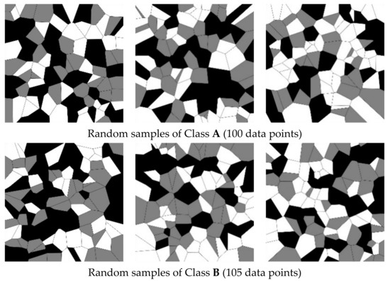
Figure 5.
Random samples of a simulated microstructure associated with Class A (top) and Class B (bottom) considered in Case Study 1. Classes A and B contain 100 and 105 data points, respectively.
It should be noted that the analysis done by the different algorithms strictly focuses on the appearance of the images, as determined by the distributions of the pixels in the images. This could be closely related to the simulated material textures in the sense of the random orientation of the simulated grains in polycrystalline materials, but it is not a direct measurement of the material texture as such. The same would apply to Case Study 2.
The convolutional neural networks used in this investigation were built using a PyTorch backend. All the experiments were run on a graphics processing unit (GPU) device on the Google Colab platform. In general, two approaches were adopted. In the first approach, Voronoi images were identified from features extracted by use of traditional algorithms including GLCM, LBP and textons.
In the second approach, Voronoi images were identified from features directly extracted by use of convolutional neural networks pretrained on images from a different domain (hereafter referred to as direct deep feature extraction), as well as partially retrained and fully retrained convolutional neural networks, including the use of AlexNet, VGG19, GoogLeNet, ResNet50 and MobileNetV2.
More specifically, with direct deep feature extraction, all froth images were passed through the abovementioned five CNNs and the features generated in the layer immediately preceding the last fully connected layer were used as predictors for classification of the froth images. By removing this last layer and freezing the weights of the model, the network can be regarded as a feature extractor. The traditional feature sets and the direct deep feature sets were then used as input to a random forest model to evaluate their corresponding classification performance to distinguish texture A from texture B.
In the partially retrained networks and fully retrained networks, the original network architecture remained unchanged, and the only difference from the direct deep feature extraction was whether to unfreeze the later layers or all the layers of the original network architecture for further retraining. The features were extracted from the same layer as that in direct deep feature extraction, that is, the layer immediately preceding the last fully connected layer.
It should be noted that for the partially retrained networks, the unfrozen layers in different CNNs are different. For AlexNet and VGG19, the weights are unfrozen from the second last convolutional blocks. For GoogLeNet, the weights are unfrozen from the second last inception modules. For ResNet50, the weights are unfrozen from the second last residual modules. For MobileNetV2, the weighs were unfrozen from the second last inverted residual blocks.
As mentioned above, random forest classification models were used in combination with the traditional feature sets and the direct deep feature sets to assess the quality of the features quantitatively. The mean value of the out-of-bag (OOB) accuracy over 30 runs was used as indicator of the classification performance. The hyperparameters used in random forest models are summarized in Table 2. The same hyperparameters were used in Case Studies 2 and 3 as well, noting that is the number of features extracted by each algorithm.
Table 2.
Hyperparameters used in random forest models.
During partial or full retraining of the CNNs, Voronoi images were randomly split into training and test datasets (split ratio 80:20), with the latter used as an independent test set to validate the generalization of the neural network models. The training set was further randomly shuffled, and 75% of it was used to train the models, while the remainder was allocated to a validation set. The adaptive momentum estimation (ADAM) algorithm [58] was used as the optimizer in this work. Hyperparameter optimization was done by use of grid search. Different optimal learning rates with or without L2 penalty apply to different CNNs. For most models, the optimal initial learning rate was 0.00001 with a weight decay parameter of 0.0000001 (L2 penalty). Optimal batch sizes and number of epochs varied as well. In order to deal with overfitting, image augmentation was used in the training stage by randomly rotating, shearing, shifting and horizontally flipping the original images. The retrained CNN models were used as end-to-end classifiers to discriminate between the two classes of simulated material textures.
Classification tasks to discriminate class A and B were performed and the corresponding features were extracted with the GLCM, LBP, textons, AlexNet (three methods: direct deep feature extraction, partially retrained, fully retrained), VGG19 (three methods: direct deep feature extraction, partially retrained, fully retrained), GoogLeNet (three methods: direct deep feature extraction, partially retrained, fully retrained), ResNet50 (three methods: direct deep feature extraction, partially retrained, fully retrained) and MobileNetV2 (three methods: direct deep feature extraction, partially retrained, fully retrained) algorithms from each of the images in the texture datasets.
The classification performance of the models is summarized in Table 3, together with the number of features associated with each model. The three methods used with each CNN algorithm are indicated as by different superscripts, for example, AlexNet, AlexNet* and AlexNet** refer to AlexNet with direct deep feature extraction, AlexNet with partial retraining and AlexNet with full retraining, respectively.
Table 3.
Comparison between different texture predictors for Case Study 1.
As can been seen from Table 3, all the traditional feature sets can discriminate between Class A and B reasonably well, with accuracies ranging from 57.69% to 64.82%. Not all the direct deep feature sets performed as well as the traditional feature sets. For example, GoogLeNet underperformed, while the others performed similarly.
As expected, the partially retrained networks improved the accuracy to at least 62.75% (only textons exceeds this value among the three traditional models), and the fully retrained networks further improved the accuracy to at least 65.75%. The best model in Case Study 1 is the fully retrained GoogLeNet, which achieved the accuracy of 74.25%. Generally, retraining of CNNs improved the classification accuracy and the depth of retraining led to further improvement.
By making use of t-SNE plots, it is possible to visualize the extracted features in a two-dimensional score space and qualitatively assess the discriminative power of the different models. The t-distributed stochastic neighbor embedding (t-SNE) [59,60] algorithm constructs the points embedded in a low-dimensional space to best approximate the relative similarities of the points in the original high-dimensional space with those in the low-dimensional space. It does so by minimizing the Kullback–Leibler divergence between the two distributions by moving the embedded points.
Figure 6 shows the t-SNE score plots of the features extracted from different methods with the corresponding classification accuracy. Retrained networks can produce better separation between two classes than the direct deep feature extraction methods and traditional feature extractors.
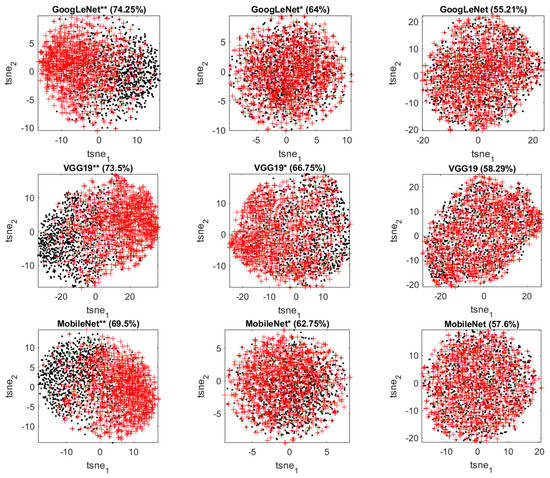
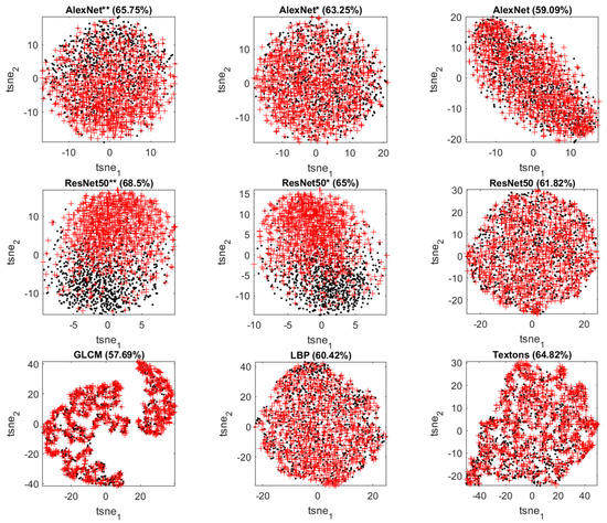
Figure 6.
t-SNE score plots of the features extracted from GoogLeNet (top panel: fully retrained, partially retrained, transfer learning), VGG19 (second panel: fully retrained, partially retrained, transfer learning), MobileNet (third panel: fully retrained, partially retrained, transfer learning), AlexNet (fourth panel: fully retrained, partially retrained, transfer learning), ResNet50 (fifth panel, fully retrained, partially retrained, transfer learning) and the traditional predictors (bottom panel: GLCM, LBP, textons) in Case Study 1. Class A is indicated by black dots and Class B by red ‘+’ markers.
With further improvement in accuracy using features extracted from fully retrained networks, the separation between Class A and B becomes clearer. From these visualization results, one can confirm that the retraining of CNNs improves the discrimination between the two classes of microstructures and the depth of retraining makes a difference.
5. Case Study 2: Voronoi-Simulated Material Microstructures of Different Grain Shape
In the second case study, both classes of simulated textures were generated with equisized datasets of 1000 samples each. Texture dataset A was generated by random sampling of a bivariate Gaussian distribution with a mean vector μ = [0,0] and a covariance matrix of Σ = [1 0; 0 1]. Texture dataset B was generated by 50%–50% random sampling of a bivariate Gaussian distribution with a mean vector μ = [−0.05,0] and a covariance matrix of Σ = [1 0; 0 1], as well as a bivariate Gaussian distribution with a mean vector μ = [+0.05,0] and a covariance matrix of Σ = [1 0; 0 1]. This different generation process means that Class B contains more elongated grains than Class A. Examples of these simulated textures are shown in Figure 7.
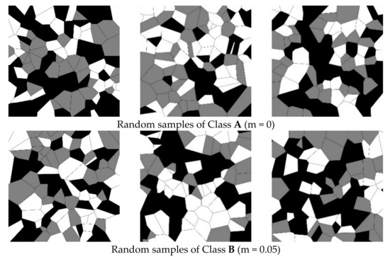
Figure 7.
Random samples of a simulated microstructure associated with Class A (top) and Class B (bottom) considered in Case Study 2. Classes A and B are generated with m = 0 and 0.05, respectively.
The same framework for classification of the different classes as Case Study 1 is used in Case Study 2. The hyperparameters for the random forest models are the same as summarized in Table 2. As the deep learning models, GoogLeNet and MobileNetV2 and the traditional texton algorithm performed best in Case Study 1, they are further considered here. The three approaches to implementation of GoogLeNet and MobileNetV2 were the same as those in Case Study 1.
The classification performance of different models in Case Study 2 is summarized in Table 4, together with the dimension of the corresponding feature set. As can be seen in Table 4, again the direct deep feature extraction methods achieve comparable performance to the traditional model textons, but neither of them can well discriminate Class A from Class B due to the low accuracies (53.54~55.74%).
Table 4.
Comparison between different texture predictors for Case Study 2.
The classification accuracy with the two retrained CNNs was improved to 63.25~64.75% for partially retraining and 70.75~72.25% for fully retraining. This observation confirms the effectiveness of retraining CNNs. Moreover, it is noteworthy that the performance of the fully retrained MobileNetV2 was comparable to that of the fully retrained GoogLeNet, considering that MobileNetV2 generally has a slightly lower accuracy, but relatively faster training speed.
To have a further visual look at how the features extracted by different methods can discriminate between the two classes of textures in Case Study 2, the t-SNE score plots with corresponding classification accuracies are shown in Figure 8. The visualization results in Case Study 2 are similar to those in Case Study 1. Fully retrained networks can produce sharper separation (less overlap) between Class A and B than partially retrained networks, followed by untrained networks and traditional predictors.
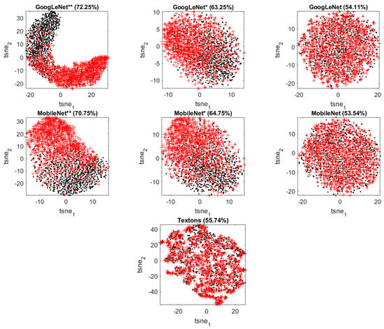
Figure 8.
t-SNE score plots of the features extracted from GoogLeNet (top panel: fully retrained, partially retrained, transfer learning), MobileNet (middle panel: fully retrained, partially retrained, transfer learning) and the traditional predictor textons (bottom panel) in Case Study 2. Class A is indicated by black dots and Class B by red ‘+’ markers.
6. Case Study 3: Real Textures in Ultrahigh Carbon Steel for Material Classification
In the final case study, a subset of the public Ultrahigh Carbon Steel Micrograph DataBase (UHCSDB) [61] of 961 scanning electron microscopy (SEM) UHCS micrographs was considered to classify the textures in terms of heat treatments or annealing conditions on spheroidite morphology. We limited the classification dataset to four annealing conditions with at least 20 micrographs under the same temperature (970 °C) and cooling method (water quench). The only difference between the four classes A–D is the annealing time, that is, 90 min, 3 h, 8 h and 24 h, respectively. The classification dataset contained 660 images and was constructed by cropping four smaller 224 × 224 pixel equalized images from the center of each original micrograph. Examples from each class are shown in Figure 9.
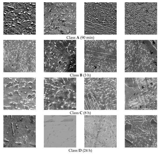
Figure 9.
Typical images of microstructures in UHCS associated with Classes A–D considered in Case Study 3. The annealing time is indicated in parentheses.
As before, the same framework for classification as used in Case Study 1 and 2 was used in Case Study 3. To minimize the variability of model performance, the two fully retrained networks were trained multiple times on several different split of training set (including the validation set) and tested on the remaining different independent test set.
The classification performance of different models in Case Study 3 is summarized in Table 5, together with the dimension of the corresponding feature set. Classification performance was based on the percentage of images correctly classified, using the feature sets as predictors. As can be seen in Table 5, one of direct deep feature extraction methods achieved comparable performance with the traditional model textons. Furthermore, the classification accuracy with the two retrained CNNs improved to 87.31~91.04% with partial retraining and near-perfect accuracies 97.01~97.76% with full retraining.
Table 5.
Comparison between different texture predictors for Case Study 3.
The performance of the fully retrained MobileNetV2 appeared to be slightly better than that of the fully retrained GoogLeNet, despite the trade-off in MobileNetV2 between performance and speed. To further highlight the performance of GoogLeNet and MobileNet, their receiver operating curves (ROC) are given in Appendix A.
As before, the features can be visualized in t-SNE score plots in Figure 10. Only one feature set of each fully retrained network (which has been trained multiple times) is shown here for visualization purposes. Textons can separate the four classes reasonably well, but overlap can still be seen between successive classes. Similarly, the CNN features extracted directly without retraining of the features layers of the networks separate the four classes and overlap exists.
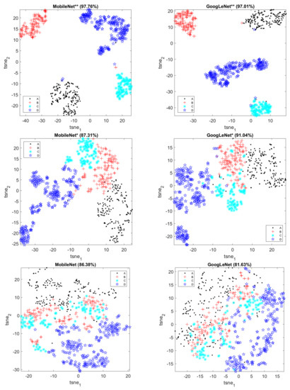
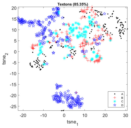
Figure 10.
t-SNE score plots of image features in Case Study 3.
The partially retrained CNN features could separate the four classes a bit better, as the four classes are generally located in a sequence of regions, although some overlap still exists for specific classes (e.g., Class B and the other classes). In contrast, the fully retrained CNN features form four distinct clusters in the feature space and thus can separate the four classes nearly perfectly.
To further demonstrate the classification performance of the fully retrained MobileNet, the confusion matrix on the test set is shown in Table 6. There are 20–48 samples for each class in the test set. The actual observations are presented in rows, while the predicted labels are presented in the columns of the table. More specifically, the numbers on the diagonal represent correct predictions, while the off-diagonal numbers give insight in the failures of the model. As can been seen from Table 6, Classes C and D can be distinguished from the other classes perfectly, while the only few errors made by the model were associated with distinguishing Class A from Class D, as well as distinguishing Class B from Class A. This is consistent with the visualization results in the corresponding t-SNE plot. This may in part be owing to the small dataset available, and the statistical variation in the images themselves, which could have contributed to the intractability of the problem.
Table 6.
Confusion matrix on test set for fully retrained MobileNet in Case Study 3.
7. Discussion
Owing to their deep architectures and large parameters sets, convolutional neural networks are displacing traditional methods in image recognition as state-of-the-art methods in an increasing number of applications. Training large and complex convolutional neural networks completely from scratch can be prohibitively costly, if sufficient data for training are available in the first place. Therefore, the use of pretrained networks is a potentially attractive approach to automated image recognition.
All three case studies demonstrate the effectiveness and superiority of using pretrained convolutional neural networks as competent feature extractors, as well as end-to-end classifiers. These pretrained networks were originally designed to capture domain-specific features from ImageNet images, which may not be optimal for classifying images from other domains (e.g., material textures). However, the case studies have shown that they are able to achieve at least equivalent (without retraining) or better performance (with partial retraining or full retraining) in texture classification compared with traditional feature extraction methods (specifically GLCM, LBP and textons).
When used directly as deep feature extractors, the classification accuracy using these features was generally similar to that obtained with the traditional algorithms in Case Studies 1 and 2, or slightly better than the latter in Case Study 3. The performance of the original deep learning models was probably inhibited by the strong dissimilarity between the source and target databases, as well as the comparatively small size of the simulated microstructure image dataset and the image dataset of ultrahigh carbon steel. Compensation for the dissimilarity and data scarcity requires retraining of the top layers or all the layers of the network.
When retraining the pretrained networks, fine tuning of the weights is accomplished by backpropagation. The earlier layers of these pretrained networks have learned more generic features that are useful for different tasks, while the later layers have learned more complex features that are more specific to the domain of the source dataset. Therefore, it is sensible to freeze the earlier layers and retrain the later layers, forcing the networks to learn high-level features that are relevant to the new dataset. Furthermore, fully retraining and unfreezing all the layers led to markedly higher accuracy in all the case studies.
In future work, other lightweight and effective convolutional neural networks (e.g., ShuffleNet and EfficientNet) for texture analysis should be explored further. Full retraining of these networks should be considered at the first place, owing to the increasing computational power of devices and improved accessibility to high-performance computing (HPC) facilities. Further advanced training strategies, based on the use of transfer learning and progressive image resizing [62], could also yield richer, hierarchical textural feature sets.
In addition, the efficacy of convolutional neural networks specifically designed for textural feature extraction would also need to be considered, as the advantages of these neural networks have not been established yet. Examples of these networks include T-CNN [63,64] and B-CNN [65], as well as Deep-TEN [66].
Finally, future work is likely to focus increasingly on the interpretation of the deep learning models [67,68]. This would not only be to increase the acceptance of a model that can explain the reason why a certain texture or image is identified, but also would potentially enhance the analyst’s understanding of physical attributes of materials that affect their performance in different applications.
8. Conclusions
In this paper, the use of pretrained convolutional neural network architectures for the quantitative analysis of both simulated and real material textures is explored. The following conclusions can be drawn.
- Architectures, such as AlexNet, VGG19, GoogLeNet, ResNet50 and MobileNetV2, pretrained on a large public common object image dataset (ImageNet), can be used directly to generate textural descriptors of similar quality as what could be achieved with engineered features, despite the fact that these networks were trained on image data from a different domain.
- As expected, further improvement is possible by partial or full retraining of all the networks. In the case studies considered in this investigation, this resulted in markedly better classification of the different simulated microstructures and the recognition of microstructures of ultrahigh carbon steel under different annealing conditions.
- All the convolutional neural networks performed as well or better than the traditional algorithms (GLCM, LBP and textons). These results are in line with those of other emerging investigations.
- Of the five abovementioned convolutional neural network architectures that were compared in the case studies, GoogLeNet and/or MobileNetV2 yielded the most reliable features. MobileNetV2 would therefore be the preferred approach, given that it trained faster than GoogLeNet.
Author Contributions
Conceptualization, C.A. and X.L.; methodology, C.A.; software, X.L.; validation, X.L. and C.A.; formal analysis, C.A. and X.L.; investigation, X.L.; resources, C.A.; data curation, X.L.; writing—original draft preparation, C.A.; writing—review and editing, C.A. and X.L.; visualization, X.L.; supervision, C.A.; project administration, C.A.; funding acquisition, C.A. All authors have read and agreed to the published version of the manuscript.
Funding
This research was supported by the Australian Research Council for the ARC Centre of Excellence for Enabling Eco-Efficient Beneficiation of Minerals, grant number CE200100009.
Institutional Review Board Statement
Not applicable.
Informed Consent Statement
Not applicable.
Data Availability Statement
The data presented in this study are available on request from the corresponding author.
Conflicts of Interest
The authors declare no conflict of interest.
Appendix A. Receiver Operating Curves for GoogLeNet and MobileNet in Case Study 3

Figure A1.
Receiver operating curves for GoogLeNet and MobileNet in Case Study 3.
Figure A1.
Receiver operating curves for GoogLeNet and MobileNet in Case Study 3.

References
- Donskoi, E.; Poliakov, A.; Holmes, R.; Suthers, S.; Ware, N.; Manuel, J.; Clout, J. Iron ore textural information is the key for prediction of downstream process performance. Miner. Eng. 2016, 86, 10–23. [Google Scholar] [CrossRef]
- Jardine, M.A.; Miller, J.A.; Becker, M. Coupled X-ray computed tomography and grey level co-occurrence matrices as a method for quantification of mineralogy and texture in 3D. Comput. Geosci. 2018, 111, 105–117. [Google Scholar] [CrossRef]
- Ghalati, M.K.; Nunes, A.; Ferreira, H.; Serranho, P.; Bernardes, R. Texture Analysis and its Applications in Biomedical Imaging: A Survey. IEEE Rev. Biomed. Eng. 2021, 15, 222–246. [Google Scholar] [CrossRef] [PubMed]
- Kerut, E.K.; Given, M.; Giles, T.D. Review of methods for texture analysis of myocardium from echocardiographic images: A means of tissue characterization. Echocardiography 2003, 20, 727–736. [Google Scholar] [CrossRef]
- Kistner, M.; Jemwa, G.T.; Aldrich, C. Monitoring of mineral processing systems by using textural image analysis. Miner. Eng. 2013, 52, 169–177. [Google Scholar] [CrossRef]
- Razavian, A.S.; Azizpour, H.; Sullivan, J.; Carlsson, S. CNN Features Off-the-Shelf: An Astounding Baseline for Recognition. In Proceedings of the 2014 IEEE Conference on Computer Vision and Pattern Recognition Workshops, Columbus, OH, USA, 23–28 June 2014; pp. 512–519. [Google Scholar]
- Fu, Y.; Aldrich, C. Froth image analysis by use of transfer learning and convolutional neural networks. Miner. Eng. 2018, 115, 68–78. [Google Scholar] [CrossRef]
- Mormont, R.; Geurts, P.; Maree, R. Comparison of Deep Transfer Learning Strategies for Digital Pathology. In Proceedings of the 2018 IEEE/CVF Conference on Computer Vision and Pattern Recognition Workshops (CVPRW), Salt Lake City, UT, USA, 18–23 June 2018; pp. 2343–234309. [Google Scholar]
- Xiao, T.; Liu, L.; Li, K.; Qin, W.; Yu, S.; Li, Z. Comparison of Transferred Deep Neural Networks in Ultrasonic Breast Masses Discrimination. Biomed. Res. Int. 2018, 2018, 4605191. [Google Scholar] [CrossRef]
- Goodall, W.R.; Scales, P.J. An overview of the advantages and disadvantages of the determination of gold mineralogy by automated mineralogy. Miner. Eng. 2007, 20, 506–517. [Google Scholar] [CrossRef]
- Pérez-Barnuevo, L.; Lévesque, S.; Bazin, C. Automated recognition of drill core textures: A geometallurgical tool for mineral processing prediction. Miner. Eng. 2018, 118, 87–96. [Google Scholar] [CrossRef]
- Zhou, J.; Gu, Y. Geometallurgical Characterization and Automated Mineralogy of Gold Ores. In Gold Ore Processing; Adams, M.D., Ed.; Elsevier: Amsterdam, The Netherlands, 2016; pp. 95–111. [Google Scholar]
- Lund, C.; Lamberg, P.; Lindberg, T. A new method to quantify mineral textures for geometallurgy. In Proceedings of the Process Mineralogy; Publisher Geology: Cape Town, South Africa, 2014. [Google Scholar]
- Anderson, K.F.E.; Wall, F.; Rollinson, G.K.; Moon, C.J. Quantitative mineralogical and chemical assessment of the Nkout iron ore deposit, Southern Cameroon. Ore Geol. Rev. 2014, 62, 25–39. [Google Scholar] [CrossRef]
- Jouini, M.S.; Keskes, N. Numerical estimation of rock properties and textural facies classification of core samples using X-ray Computed Tomography images. Appl. Math. Model. 2017, 41, 562–581. [Google Scholar] [CrossRef]
- Tungpalan, K.; Wightman, E.; Manlapig, E. Relating mineralogical and textural characteristics to flotation behaviour. Miner. Eng. 2015, 82, 136–140. [Google Scholar] [CrossRef]
- Parian, M.; Mwanga, A.; Lamberg, P.; Rosenkranz, J. Ore texture breakage characterization and fragmentation into multiphase particles. Powder Technol. 2018, 327, 57–69. [Google Scholar] [CrossRef]
- Voigt, M.; Miller, J.A.; Mainza, A.N.; Bam, L.C.; Becker, M. The Robustness of the Gray Level Co-Occurrence Matrices and X-ray Computed Tomography Method for the Quantification of 3D Mineral Texture. Minerals 2020, 10, 334. [Google Scholar] [CrossRef]
- Partio, M.; Cramariuc, B.; Gabbouj, M.; Visa, A. Rock Texture Retrieval Using Gray Level Co-occurrence Matrix. In Proceedings of the 5th Nordic Signal Processing Symposium (NORSIG 2002), Hurtigruten, Norway, 4–7 October 2002. [Google Scholar]
- Leigh, G.M. Automatic Ore Texture Analysis for Process Mineralogy. In Proceedings of the Ninth International Congress for Applied Mineralogy (ICAM Australia 2008), Brisbane, QLD, Australia, 8–10 September 2008; pp. 433–435. [Google Scholar]
- Koch, P.-H. Particle Generation for Geometallurgical Process Modeling. Ph.D. Thesis, Luleå Tekniska Universitet, Luleå, Sweden, 2017. [Google Scholar]
- Fu, Y.; Aldrich, C. Quantitative Ore Texture Analysis with Convolutional Neural Networks. IFAC-Pap. 2019, 52, 99–104. [Google Scholar] [CrossRef]
- Renzetti, F.R.; Zortea, L. Use of a gray level co-occurrence matrix to characterize duplex stainless steel phases microstructure. Frat. Ed Integrità Strutt. 2011, 5, 43–51. [Google Scholar] [CrossRef]
- Webel, J.; Gola, J.; Britz, D.; Mücklich, F. A new analysis approach based on Haralick texture features for the characterization of microstructure on the example of low-alloy steels. Mater. Charact. 2018, 144, 584–596. [Google Scholar] [CrossRef]
- Velichko, A.; Holzapfel, C.; Siefers, A.; Schladitz, K.; Mücklich, F. Unambiguous classification of complex microstructures by their three-dimensional parameters applied to graphite in cast iron. Acta Mater. 2008, 56, 1981–1990. [Google Scholar] [CrossRef]
- DeCost, B.L.; Francis, T.; Holm, E.A. Exploring the microstructure manifold: Image texture representations applied to ultrahigh carbon steel microstructures. Acta Mater. 2017, 133, 30–40. [Google Scholar] [CrossRef]
- Azimi, S.M.; Britz, D.; Engstler, M.; Fritz, M.; Mucklich, F. Advanced Steel Microstructural Classification by Deep Learning Methods. Sci. Rep. 2018, 8, 2128. [Google Scholar] [CrossRef]
- Gola, J.; Webel, J.; Britz, D.; Guitar, A.; Staudt, T.; Winter, M.; Mücklich, F. Objective microstructure classification by support vector machine (SVM) using a combination of morphological parameters and textural features for low carbon steels. Comput. Mater. Sci. 2019, 160, 186–196. [Google Scholar] [CrossRef]
- Beniwal, A.; Dadhich, R.; Alankar, A. Deep learning based predictive modeling for structure-property linkages. Materialia 2019, 8, 100435. [Google Scholar] [CrossRef]
- Trambitckii, K.; Anding, K.; Polte, G.; Garten, D.; Musalimov, V.; Kuritcyn, P. The application of texture features to quality control of metal surfaces. Acta IMEKO 2016, 5, 19. [Google Scholar] [CrossRef][Green Version]
- Medeiros, F.N.S.; Ramalho, G.L.B.; Bento, M.P.; Medeiros, L.C.L. On the Evaluation of Texture and Color Features for Nondestructive Corrosion Detection. EURASIP J. Adv. Signal Process. 2010, 2010, 817473–817478. [Google Scholar] [CrossRef]
- Guo, Y.; Sun, Z.; Sun, H.; Song, X. Texture feature extraction of steel strip surface defect based on gray level co-occurrence matrix. In Proceedings of the 2015 International Conference on Machine Learning and Cybernetics (ICMLC), Guangzhou, China, 12–15 July 2015; pp. 217–221. [Google Scholar]
- Luo, Q.; Fang, X.; Sun, Y.; Liu, L.; Ai, J.; Yang, C.; Simpson, O. Surface Defect Classification for Hot-Rolled Steel Strips by Selectively Dominant Local Binary Patterns. IEEE Access 2019, 7, 23488–23499. [Google Scholar] [CrossRef]
- Mao, S.; Natarajan, V.; Chia, L.-T.; Huang, G.-B. Texture Recognition on Metal Surface using Order-Less Scale Invariant GLAC. In Proceedings of the 2019 IEEE 31st International Conference on Tools with Artificial Intelligence (ICTAI), Portland, OR, USA, 4–6 November 2019; pp. 629–635. [Google Scholar]
- Das, P.; Dutta, S.; Roy, H.; Rengaswamy, J. Characterization of Impact Fracture Surfaces Under Different Processing Conditions of 7075 Al Alloy using Image Texture Analysis. Int. J. Technol. Eng. Syst. 2011, 2, 143–147. [Google Scholar]
- Dutta, S.; Das, A.; Barat, K.; Roy, H. Automatic characterization of fracture surfaces of AISI 304LN stainless steel using image texture analysis. Measurement 2012, 45, 1140–1150. [Google Scholar] [CrossRef]
- Dutta, S.; Barat, K.; Das, A.; Das, S.K.; Shukla, A.K.; Roy, H. Characterization of micrographs and fractographs of Cu-strengthened HSLA steel using image texture analysis. Measurement 2014, 47, 130–144. [Google Scholar] [CrossRef]
- Naik, D.L.; Kiran, R. Identification and characterization of fracture in metals using machine learning based texture recognition algorithms. Eng. Fract. Mech. 2019, 219, 106618. [Google Scholar] [CrossRef]
- Müller, A.; Karathanasopoulos, N.; Roth, C.C.; Mohr, D. Machine Learning Classifiers for Surface Crack Detection in Fracture Experiments. Int. J. Mech. Sci. 2021, 209, 106698. [Google Scholar] [CrossRef]
- Bastidas-Rodriguez, M.X.; Prieto-Ortiz, F.A.; Espejo, E. Fractographic classification in metallic materials by using computer vision. Eng. Fail. Anal. 2016, 59, 237–252. [Google Scholar] [CrossRef]
- Dutta, S.; Karmakar, A.; Roy, H.; Barat, K. Automatic estimation of mechanical properties from fractographs using optimal anisotropic diffusion and Voronoi tessellation. Measurement 2019, 134, 574–585. [Google Scholar] [CrossRef]
- Haralick, R.M.; Shanmugam, K.; Dinstein, I.H. Textural Features for Image Classification. IEEE Trans. Syst. Man Cybern. 1973, SMC-3, 610–621. [Google Scholar] [CrossRef]
- Moolman, D.W.; Aldrich, C.; van Deventer, J.S.J.; Stange, W.W. Digital image processing as a tool for on-line monitoring of froth in flotation plants. Miner. Eng. 1994, 7, 1149–1164. [Google Scholar] [CrossRef]
- Moolman, D.W.; Aldrich, C.; van Deventer, J.S.J. The monitoring of froth surfaces on industrial flotation plants using connectionist image processing techniques. Miner. Eng. 1995, 8, 23–30. [Google Scholar] [CrossRef]
- Moolman, D.W.; Aldrich, C.; van Deventer, J.S.J.; Bradshaw, D.J. The interpretation of flotation froth surfaces by using digital image analysis and neural networks. Chem. Eng. Sci. 1995, 50, 3501–3513. [Google Scholar] [CrossRef]
- Ojala, T.; Pietikäinen, M.; Harwood, D. A comparative study of texture measures with classification based on featured distributions. Pattern Recognit. 1996, 29, 51–59. [Google Scholar] [CrossRef]
- Mansano, M.; Pavesi, L.; Oliveira, L.S.; Britto, A.; Koerich, A. Inspection of metallic surfaces using Local Binary Patterns. In Proceedings of the IECON 2011—37th Annual Conference of the IEEE Industrial Electronics Society, Melbourne, VIC, Australia, 7–10 November 2011; pp. 2227–2231. [Google Scholar]
- Fu, Y.; Aldrich, C. Flotation Froth Image Analysis by Use of a Dynamic Feature Extraction Algorithm. IFAC-PapersOnLine 2016, 49, 84–89. [Google Scholar] [CrossRef]
- Aldrich, C.; Smith, L.K.; Verrelli, D.I.; Bruckard, W.J.; Kistner, M. Multivariate image analysis of realgar–orpiment flotation froths. Mineral. Process. Extr. Metall. 2017, 127, 146–156. [Google Scholar] [CrossRef]
- Aldrich, C.; Uahengo, F.D.L.; Kistner, M. Estimation of particle size in hydrocyclone underflow streams by use of Multivariate Image Analysis. Miner. Eng. 2015, 70, 14–19. [Google Scholar] [CrossRef]
- Leung, T.; Malik, J. Representing and Recognizing the Visual Appearance of Materials using Three-dimensional Textons. Int. J. Comput. Vis. 2001, 43, 29–44. [Google Scholar] [CrossRef]
- Schmid, C. Constructing models for content-based image retrieval. In Proceedings of the 2001 IEEE Computer Society Conference on Computer Vision and Pattern Recognition (CVPR 2001), Kauai, HI, USA, 8–14 December 2001; pp. 39–45. [Google Scholar]
- Varma, M.; Zisserman, A. A statistical approach to material classification using image patch exemplars. IEEE Trans. Pattern. Anal. Mach. Intell. 2009, 31, 2032–2047. [Google Scholar] [CrossRef]
- Jemwa, G.T.; Aldrich, C. Estimating size fraction categories of coal particles on conveyor belts using image texture modeling methods. Expert Syst. Appl. 2012, 39, 7947–7960. [Google Scholar] [CrossRef]
- Krizhevsky, A.; Sutskever, I.; Hinton, G.E. ImageNet classification with deep convolutional neural networks. Commun. ACM 2017, 60, 84–90. [Google Scholar] [CrossRef]
- Szegedy, C.; Liu, W.; Jia, Y.; Sermanet, P.; Reed, S.; Anguelov, D.; Erhan, D.; Vanhoucke, V.; Rabinovich, A. Going Deeper with Convolutions. In Proceedings of the 2015 IEEE Conference on Computer Vision and Pattern Recognition (CVPR), Boston, MA, USA, 7–12 June 2015; pp. 1–9. [Google Scholar]
- Sandler, M.; Howard, A.; Zhu, M.; Zhmoginov, A.; Chen, L.-C. MobileNetV2: Inverted Residuals and Linear Bottlenecks. In Proceedings of the 2018 IEEE/CVF Conference on Computer Vision and Pattern Recognition (CVPR), Salt Lake City, UT, USA, 18–23 June 2018; pp. 4510–4520. [Google Scholar]
- Kingma, D.P.; Ba, J. Adam: A Method for Stochastic Optimization. In Proceedings of the Published as a Conference Paper at the 3rd International Conference on Learning Representations, San Diego, CA, USA, 7–9 May 2015. [Google Scholar]
- Hinton, G.; Roweis, S. Stochastic Neighbor Embedding. Adv. Neural Inf. Process. Syst. 2003, 15, 857–864. [Google Scholar]
- van Der Maaten, L.; Hinton, G. Visualizing data using t-SNE. J. Mach. Learn. Res. 2008, 9, 2579–2625. [Google Scholar]
- DeCost, B.L.; Hecht, M.D.; Francis, T.; Webler, B.A.; Picard, Y.N.; Holm, E.A. UHCSDB: UltraHigh Carbon Steel Micrograph DataBase. Integr. Mater. Manuf. Innov. 2017, 6, 197–205. [Google Scholar] [CrossRef]
- Bhatt, A.; Ganatra, A.; Kotecha, K. COVID-19 pulmonary consolidations detection in chest X-ray using progressive resizing and transfer learning techniques. Heliyon 2021, 7, e07211. [Google Scholar] [CrossRef]
- Andrearczyk, V.; Whelan, P.F. Using filter banks in Convolutional Neural Networks for texture classification. Pattern. Recognit. Lett. 2016, 84, 63–69. [Google Scholar] [CrossRef]
- Wu, H.; Yan, W.; Li, P.; Wen, Z. Deep Texture Exemplar Extraction Based on Trimmed T-CNN. IEEE Trans. Multimed. 2021, 23, 4502–4514. [Google Scholar] [CrossRef]
- Lin, T.; RoyChowdhury, A.; Maji, S. Bilinear CNN Models for Fine-Grained Visual Recognition. In Proceedings of the 2015 IEEE International Conference on Computer Vision (ICCV), Santiago, Chile, 11–18 December 2015; pp. 1449–1457. [Google Scholar]
- Zhang, H.; Xue, J.; Dana, K. Deep TEN: Texture Encoding Network. In Proceedings of the 2017 IEEE Conference on Computer Vision and Pattern Recognition (CVPR), Honolulu, HI, USA, 21–26 July 2017; pp. 2896–2905. [Google Scholar]
- Joshi, G.; Walambe, R.; Kotecha, K. A Review on Explainability in Multimodal Deep Neural Nets. IEEE Access 2021, 9, 59800–59821. [Google Scholar] [CrossRef]
- Pilania, G. Machine learning in materials science: From explainable predictions to autonomous design. Comput. Mater. Sci. 2021, 193, 110360. [Google Scholar] [CrossRef]


Publisher’s Note: MDPI stays neutral with regard to jurisdictional claims in published maps and institutional affiliations. |
© 2022 by the authors. Licensee MDPI, Basel, Switzerland. This article is an open access article distributed under the terms and conditions of the Creative Commons Attribution (CC BY) license (https://creativecommons.org/licenses/by/4.0/).