Abstract
Residual stresses induced by the welding processes may, in some cases, result in significant warping and distortions that can endanger the integrity of the welded structures. This document reports an investigation of the welding process to make a dissimilar T-joint through an advanced Finite Element (FE) modelling and a dedicated laboratory test. The T-joint consisted of two plates of dissimilar materials, AISI304 and S275JR steels, both having a thickness of 5 mm, welded through a Shielded Metal Arc Welding (SMAW). Thermocouples were used to acquire the temperature variations during welding. In parallel, an FE model was built and the welding process was simulated through the “element birth and death” technique. Numerical and experimental outcomes were compared in terms of temperature distributions during welding and in terms of distortion at the end of the final cooling, showing that the FE model was able to provide a high level of accuracy.
1. Introduction
Welding is a widespread joining technique used in the field of engineering due to its advantages offered in terms of design flexibility, costs, and weight saving. Several welding techniques have been developed throughout the years, and nowadays, their advancement is still of great interest for many industrial sectors [1,2,3]. All of these techniques require a high heat to melt the parts together and, very often, this represents one of the biggest downsides given by this joining technology. This is due to the high heat fluxes that can lead to several critical issues such as high residual stresses [4], inaccurate weld bead morphology [5], and distortions of the welded components [6] that in turn, can compromise the efficiency and the performance of welded structures.
Among these, residual stresses and distortions induced by the localized high heating and the subsequent cooling phases play a very critical role and their accurate estimates have to be carefully taken into account by welding engineers. Some examples of these critical aspects can be found in the literature [7,8] with reference to residual stresses after friction stir welding or laser-welded joints [9] but with reference to various fields of application, e.g., in the nuclear industry [10,11], the railway industry [12,13], or the aerospace industry [14].
The accurate evaluation of residual stresses induced by the fusion arc welding of steel joints is of great interest, especially for applications in power plants, where welded joints made of dissimilar materials are widely used to connect ferritic steel components and austenitic steel piping systems.
In recent years, destructive and non-destructive techniques have been developed to obtain information regarding the stress–strain levels in welded structures in terms of both amplitude and distribution. However, their level of accuracy does not allow for the obtaining very accurate information, and the latest advances in numerical simulation can be very helpful in this regard [15,16].
The numerical evaluation of residual stresses in dissimilar welded joints is generally more challenging than in similar ones because of the differences in terms of thermo-mechanical and metallurgical properties of the materials being joined join. Over the last two decades, there have been significant research activities focusing on the assessment of welding residual stresses in both similar and dissimilar steel welded joints through the usage of the Finite Element Method (FEM) [17].
In the literature [18], a Finite Element (FE) model, based on the birth and death element technique, was developed for predicting the welding-induced residual stresses in large structures by using a prescribed temperature field. Still leveraging on the element birth and death technique, FE models for simulating the welding process in both butt and T-joints are available in the literature [19]. Additionally, simplified methods for simulating the T-joint welding process by considering a hybrid sequential thermo-mechanical approach, in which the thermal and mechanical analyses were carried out simultaneously, can be found [20]. Some members of the same research group presented a hybrid shell/3D technique to improve the computational efficiency and accuracy of welded T-joint process simulations [21]. Validated through experimental data, this hybrid technique was characterized by the transition from shell elements to 3D elements, discretized with a finer mesh, defined according to dedicated stress criteria. Thanks to this technique, it was possible to save up to 40% of the total computational burden, even if the highest accuracy was not always guaranteed. Finally, a benchmark study [22] of uncertainness in Flux Core Arc Welding (FCAW) process simulations was conducted by proposing FE models that were based on the birth and death technique and adopted sequentially coupled thermal stress analyses. Besides all of the proposed numerical frameworks, all of these contributions only considered welding joints made of similar materials.
In terms of joints of dissimilar materials, welding residual stresses were evaluated for a dissimilar pipe joint made of A240-TP304 stainless steel and A106- B carbon steel by using a full 3D FE model [23]. A simplified methodology to compute the residual stresses in a dissimilar metal pipe joint by considering cladding, buttering, post weld heat treatment, and multi-pass welding can also be found in the literature [24]. Once more, 3D transient computational thermal models using a sliding mesh for investigating the heat transfer effects during a Friction Stir Welding (FSW) in a dissimilar T-joint were also studied [25]. Generally speaking, the use of FE models based on the element birth and death technique to calculate the residual stresses distribution in butt-welded joints of dissimilar materials has been an interesting topic for many researchers [26,27,28,29]. Finally, the FE simulation of residual stresses induced by arc welding for a P92 steel pipe using a nickel-based alloy (IN625) as filler material were also studied [30].
This document relies on the framework of the computational methods for the simulation of welding process [23,24,25,26,27,28,29,30,31,32,33,34,35,36]. Particularly, the current investigation deals with the development of an FE model for the prediction of residual stresses in welded T-joints made of dissimilar materials, namely AISI 304 stainless steel for the web and S275JR carbon steels for the flange. This work represents an advancement with reference to the investigation already published and comprising of a numerical procedure only [31]. This particular procedure was developed by means of the ABAQUS® code [36] and has already been published by some of the authors [29,31]. The welding process considered in this work referred to a Shielded Metal Arc Welding (SMAW) technique to make a dissimilar T-joint with two weld beads between the web and flange, one for each side of the T. An experimental test was carried out in a laboratory environment with temperature recorded during the welding process by means of thermocouples placed on the flange and web close to the welding line. Each weld bead was made in a single-pass with a nearly uniform speed and at room temperature.
The rest of this document is organized as it follows.
Section 2 presents the considered materials and methods together with the information regarding the experimental test carried out in laboratory. Section 3 reports the description of the FEM procedure and the element birth and death technique. The reader is also referred to the literature for further information about these aspects [29,31,36]. Section 4 presents a numerical-experimental comparison on the obtained results and a discussion on them. Finally, Section 5 concludes with the remarks of this article.
2. Materials and Methods
The welded T-joint shown in Figure 1 was made in a laboratory environment. The joint was created using an AISI 304 stainless steel plate, which was used for the web welded to a S275JR carbon steel plate, which was used for the flange. Two welding beads were used for the T-joint, one for each side, using the E 308 L-17 stainless steel as filler material.
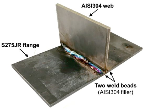
Figure 1.
AISI 304-S275JR steel T-joint.
Figure 2 presents the drawings of the joint with the locations of the thermocouples that were used to record the temperatures during the entire welding process. Particularly, six thermocouples were placed on the flange, and one was placed on the web to monitor the temperature variation during the welding sequence at various distances from the weld beads and on both web sides.
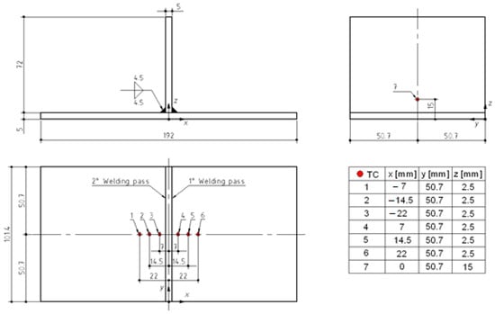
Figure 2.
Plate dimensions and layout of thermocouples; “TC” stands for thermocouple.
The final experimental set-up with a highlight on the thermocouple positioning is shown in Figure 3. It is worth mentioning that the flange was simply supported on the two sides, as shown in Figure 3, during the welding to allow for the expected distortion induced by the heavy localized heat loads created by the welding torch. The web was kept in the requested position with a magnetic support.
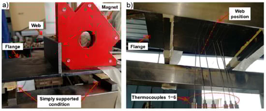
Figure 3.
Experimental set-up before welding: (a) upside and (b) underside views.
The adopted welding technique was SMAW, with the welding pass performed at nearly uniform speed and under room conditions using a 2.5 mm diameter flux-coated SMAW electrode ESAB OK 61.30 (AWS A5.4-98-E 308 L-17). A cooling phase of 179 s was experimentally needed by the operator in between the two weldments.
The heat input per unit of weld length, H, supplied by the welding torch, was defined through the following Equation (1):
where η is the welding efficiency, V is the voltage, I is the electrical current, and v is the welding speed. These data were reported in Table 1.

Table 1.
Welding process parameters.
The energy Qw supplied to the welding bead during the simulation was set up as equal to:
where Lbead was the length of the beads [29].
Qw = H∙Lbead,
3. Numerical Model
FEM thermal stress analyses were performed to replicate the welding process numerically. The numerical thermal-mechanical analyses were performed using an uncoupled approach consisting of two consecutive analyses: the first was used to predict the transient temperature field independently, whereas the second was used to calculate the stress–strain fields considering the previously computed temperature field as input data. This is a common practice for this type of calculations since it allows for the reduction of the computational effort required by a coupled temperature-displacement approach [7,8,10,11].
The weld bead formation simulation was based on the element birth and death technique. Concerning the mesh, a full 3D model was preferred. In particular, 8-noded brick elements, type DC3D8, were selected from the ABAQUS library [35] for the thermal analysis since we were considering the temperature as a unique degree of freedom for each node. Subsequently, the C3D8 8-noded brick finite elements presenting three translational degrees of freedom for each node were substituted for the DC3D8 for the mechanical analysis while keeping the same mesh size and shape. The finest mesh was built up for the chamfer region, with a linear grading through the Heat Affected Zone (HAZ), as shown in Figure 4. Finally, the FE model comprised of a total of nearly 12,000 elements and nearly 15,000 nodes.
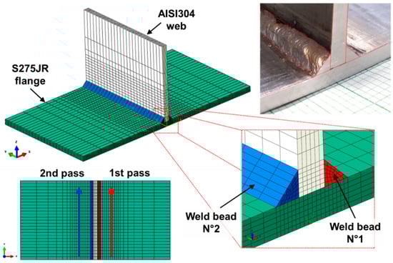
Figure 4.
Finite Element (FE) mesh highlighting the mesh grading and the two weld beads.
The two weld beads were explicitly modelled as shown in Figure 4. Using the birth and death technique, the first step of the analysis comprised of the deactivation of the weld bead elements in order to activate them along with the simulation in such a way so as to simulate the weld bead formation during the welding process. The deactivation process was implemented by multiplying the element’s stiffness by a severe reduction factor (e.g., 1e–6), thus excluding the bead elements from the analysis. These elements were combined with 26 groups of elements that were progressively reactivated during the simulation at given time intervals. This reactivation was achieved by removing the reduction factor according to the welding speed v [29].
Material properties for the base materials and filler were taken from the literature and were reported here in Figure 5 and Figure 6 for the sake of clarity [23,37,38,39]. Figure 5 and Figure 6 present the temperature-dependent thermal conductivity, specific heat, Young’s modulus, thermal expansion coefficient, and stress–strain curves for both materials. Poisson’s ratio was kept as temperature independent and was equal to 0.3 for all materials. In order to take into account of the transformation phase in the thermal analysis, a latent heat per mass unit, a solidus temperature, and a liquidus temperature equal to 277,000 J/kg, 1495 °C, 1540 °C and 277,000 J/kg, 1450 °C, 1595 °C were used for S275JR and AISI 304, respectively.
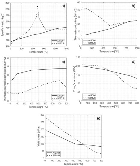
Figure 5.
Main thermal and mechanical properties for AISI304 and S275JR: (a) specific heat, (b) thermal conductivity, (c) thermal expansion coefficient, (d) Young’s modulus and (e) yield stress.
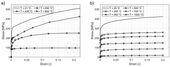
Figure 6.
Temperature-dependent stress–strain curves for (a) AISI304 and (b) S275JR.
The input thermal energy Qw (Table 1) was applied as a volumetric flux to each group of bead elements for a total time equal to tweld for each weld bead and tweld being the time needed to cover the length of each bead. The two weld beads were created sequentially according to timing measured during the laboratory test. Before starting the simulation of the second bead, a cooling phase lasting 179 s was added to simulate the cooling time elapsed between the two operations. Finally, a load step of nearly 35 min was added to conclude the analysis and simulate the final cooling down of the plates at a room temperature of nearly 40 °C.
According to some studies, the influence of phase transformations on residual stresses is negligible, for others, it is not. The solid-state austenite–martensite transformation during the cooling phase can be neglected for steel with low equivalent carbon content, as is the case with S275 JR steel. This aspect has been well demonstrated by Cho and Kim [40] and by Deng [41], where the modelling of the transformation phase does not change the level of accuracy of the FE model in terms of residual stresses and distortions prediction when the welding process involves low carbon steels. Moreover, other authors Danielewski et al. [42] and Deng et al. [24] have neglected metallurgical transformations in their work regarding the welding of dissimilar materials. As a result, the solid-state transformation phase has not been considered in the FE model.
Concerning the boundary conditions, specific film conditions were applied on the free-surfaces of the plates in order to simulate the heat transfer within the environment (the convective and radiative heat losses). A unique temperature dependent convective film coefficient (Figure 7) was introduced in the model for such a purpose, calculated as the sum of the temperature dependent convective and radiative film coefficients. All of the thermal-mechanical properties were introduced in the FE model as a function of the temperature (Figure 5 and Figure 6). Simply supported boundary conditions were considered to constrain the flange, as in Figure 3, whereas the related conductive heat loss was neglected. This did not present an element of approximation since very low temperatures (close to room temperature) were computed numerically far from the welding zone. Wood pieces were used experimentally as thermal isolators to support the flange, see Figure 3.
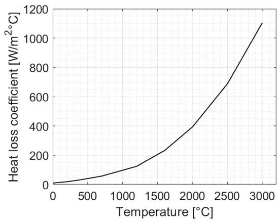
Figure 7.
Heat loss convective and radiative coefficient.
4. Results and Discussion
Figure 8 shows some frames captured during the FEM thermal where it can be noticed that the bead elements were partially reactivated, simulating the explicit weld bead formation.
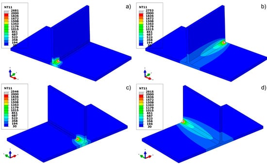
Figure 8.
Temperature distributions (°C) during welding at various simulation frames: (a) at the beginning of the first pass, (b) at the end of the first pass, (c) at the beginning of second pass, (d) at the end of the second pass.
The temperature distributions and the measured residual distortions obtained experimentally and numerically were cross-compared, especially for the validation of the numerical model. This was useful so as to give the welding engineers the option of speculating on further numerical results, e.g., the residual stresses and distortions.
Concerning the thermal results, temperature histories were measured for the nodes located in proximity to the thermocouples adopted during the experimental tests (Figure 2). Figure 9 and Figure 10 compare the temperature trends predicted at these nodes with the temperatures recorded experimentally at the same locations for the flange and web, respectively.
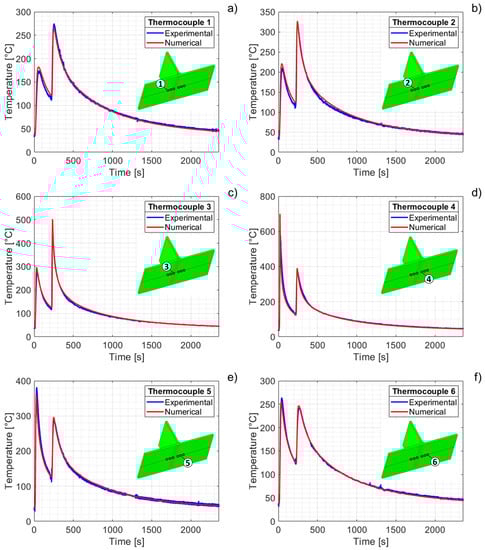
Figure 9.
Experimental vs. numerical temperature distributions at the thermocouples locations on the flange: (a–f) for thermocouple positions 1–6.
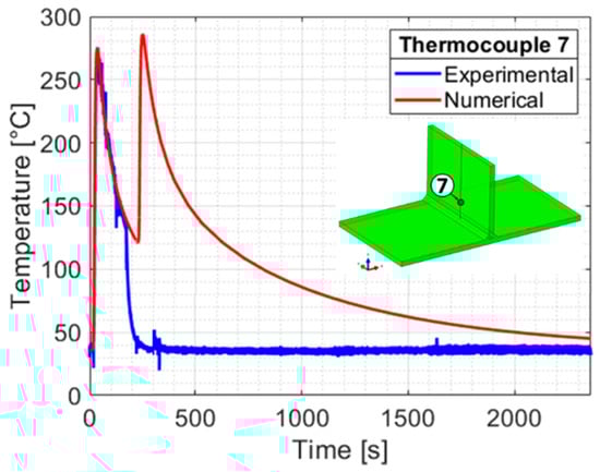
Figure 10.
Experimental vs. numerical temperature distribution at the thermocouple location on the web (Point 7).
It is worth noting that the variations in temperature versus time presented the same tendency for all of the evaluation points. During the first pass, before the welding started, the temperature remained close to the room temperature (~40 °C). When the welding torch approached the cross section at y = 50.7 mm (t = 18.1 s), the temperatures at points 4, 5, and 6 reached higher values than those at points 1, 2 and 3. This is due to the fact that those points were closer to the welding torch. At the end of the first pass, the temperature of plates was of nearly 70 °C, thus still higher than the room temperature. Similarly, when the welding torch approached the cross section at y = 50.7 mm (t = 230.1 s) during the second pass, the temperatures at these points increased to their maximum values and at different rates. Temperature values at points 1, 2, and 3 (placed closer to the welding torch) were higher than those at points 4, 5, and 6 (placed on the opposite side and farther from the welding torch).
The temperature values at points 4, 5, and 6, placed slightly closer to the welding torch during the first pass, were higher than those at points 1, 2, and 3, placed on the opposite side and farther from the torch. As the torch moved away from the cross section (t > 18.1 s), temperatures at these points decreased gradually at different rates.
It is worth noting that very similar results were shown when comparing the numerical and experimental temperatures for all of the measuring positions. Experimental and numerical curves appeared overlap with small differences only at the peak values and for the measuring points closer to the weld bead (Points 2 and 3). This was attributed to some slight discrepancies between the numerical energy Qw supplied to the weld bead and that was experimentally supplied by the welding machine.
Finally, the thermocouple in position 7 (on the web) was removed before the beginning of the second welding pass, and the comparison was only partially obtained. However, similar results were achieved for the first pass (Figure 10).
Figure 11 shows the comparison between the numerical temperature distribution along transverse direction and the experimental values of temperature recorded by thermocouples positioned on the flange. The centre of the welding arc was positioned at y = 50.7 mm (midsection) at time t = 18.1 s, i.e., during the first welding pass. Similarly, Figure 12 shows the comparison between numerical and experimental temperature distributions during the second welding pass, when the welding arc was positioned at the midsection at time t = 230.1 s. It was possible to deduce that during both passes, the experimental and numerical temperature distribution curves were mostly overlapped. This confirmed the accuracy of the numerical model in accurately simulating the thermal behaviour of the joint during the welding process.
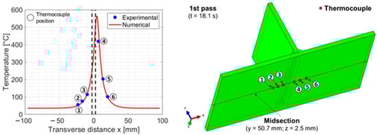
Figure 11.
Experimental vs. numerical transverse temperature distributions in the flange in midsection (y = 50.7 mm and z = 2.5 mm) at time t = 18.1 s during the first welding pass.
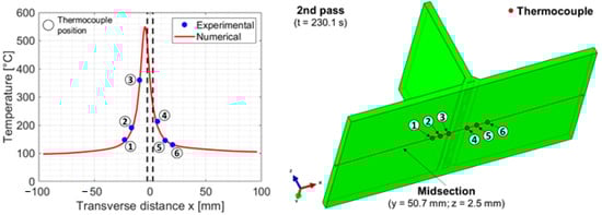
Figure 12.
Experimental vs. numerical transverse temperature distributions in the flange in midsection (y = 50.7 mm and z = 2.5 mm) at time t = 230.1 s during the second welding pass.
As it can be seen from Figure 9, Figure 10, Figure 11 and Figure 12, the peaks of temperature around the welding arc suggested that the material melted in the Fusion Zone (FZ), while high temperatures were achieved near the FZ, defining the Heat Affected Zone (HAZ). During the first pass, the highest temperature values were calculated for positions 1–3, whereas the reverse happened for positions 4–6 during the second pass. This was expected considering the different positions of the welding torch, i.e., the heat source, with reference to the web. Figure 13 compared the numerical FZ and HAZ and the experimental observations obtained through an optical micrograph. Even if only from a qualitative standpoint, the geometry and shape of both weld beads and HAZ seemed to be well captured numerically. Namely, the HAZ was defined as the section reaching a temperature higher than 727 °C during the welding process, namely the temperature of the austenite transformation. Through this comparison, it was possible to state that the used methodology was suitable to accurately predict the temperature distributions in the welded joint without the need to perform any fine tuning processes for the heat source calibration.
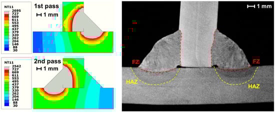
Figure 13.
Numerical-experimental comparison of heat-affected zone (HAZ). FZ: fusion zone.
The mechanical analysis was performed in order to predict the displacement values at the extremities of the flange, namely the distortions caused by the heavy localized heat loads induced by the welding process. Figure 14 shows a comparison of the distortions ∆u1 and ∆u2 measured at the end of the last cooling phase, which was nearly 35 min long, between the numerical model and the test article. Table 2 resumed the distortion values at the extremity of the flange, according to Figure 14.
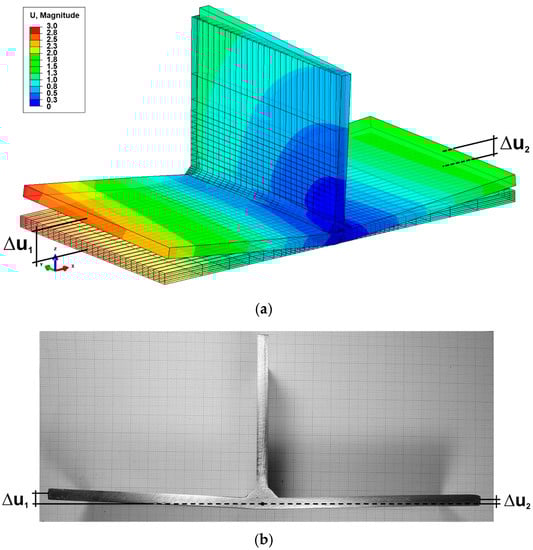
Figure 14.
(a) Numerical vs. (b) experimental displacements at the end of the cooling phase at mid-section of the joint; numerical displacements in [mm].
Table 2.
Residual distortion comparison.
It is possible to observe that the residual distortions calculated numerically were in close in value to the experimental ones. However, in more detail, the difference between the experimental and numerical distortions was only judged as sufficient. It can be therefore stated that the numerical model was able to predict the mechanical behaviour of the joint in terms of the residual distortions, even though further investigation is still needed. Finally, Figure 15 shows the longitudinal and transversal residual stresses calculated numerically. Although these stress fields are directly connected with the residual displacements field (this latter field presenting non-remarkable numerical-experimental similarities), it is possible to observe very high stress levels that cannot be neglected when evaluating the safety of the welded structures. Furthermore, numerical distortions turned out to be more conservative than the measurements, therefore even higher stresses are expected in the actual welded structures.
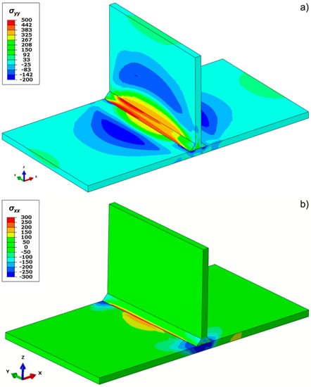
Figure 15.
(a) Longitudinal σyy and (b) transversal σxx residual stresses [MPa] calculated numerically.
5. Conclusions
This paper presented a numerical FE model to simulate the welding process to realise a T-joint made of dissimilar materials. The thermo-mechanical response was carried out using an uncoupled thermal-mechanical approach in combination with the element birth and death technique used to simulate the explicit weld bead formation during welding.
The reliability of the FEM procedure has been demonstrated through similar results between the numerical and experimental outcomes in terms of the temperature distribution and distortions of the welded joint. In particular, the temperatures field has been measured during the welding process by means of seven thermocouples placed in the proximity of the weld bead, whereas the final distortion has been measured at the end of the final cooling. The similarity of results between numerical and experimental results demonstrates the effectiveness of the proposed FEM procedure.
Author Contributions
Conceptualization, R.S. and A.D.L.; methodology, A.G.; software, A.G.; validation, V.G., R.S. and A.D.L.; formal analysis, A.G.; investigation, A.G.; resources, R.S.; data curation, V.G.; writing—original draft preparation, A.G.; writing—review and editing, V.G.; visualization, V.G.; supervision, R.S. All authors have read and agreed to the published version of the manuscript.
Funding
This research received no external funding.
Institutional Review Board Statement
Not applicable.
Informed Consent Statement
Not applicable.
Data Availability Statement
Data supporting the reported results can be obtained from the author upon request.
Conflicts of Interest
The authors declare no conflict of interest.
References
- Caiazzo, F.; Alfieri, V.; Corrado, G.; Argenio, P.; Barbieri, G.; Acerra, F.; Innaro, V. Laser Beam Welding of a Ti–6Al–4V Support Flange for Buy-to-Fly Reduction. Metals 2017, 7, 183. [Google Scholar] [CrossRef]
- Caiazzo, F.; Alfieri, V.; Sergi, V.; Schipani, A.; Cinque, S. Dissimilar autogenous disk-laser welding of Haynes 188 and Inconel 718 superalloys for aerospace applications. Int. J. Adv. Manuf. Technol. 2013, 68, 1809–1820. [Google Scholar] [CrossRef]
- Caiazzo, F.; Alfieri, V.; Corrado, G.; Cardaropoli, F.; Sergi, V. Investigation and Optimization of Laser Welding of Ti-6Al-4 V Titanium Alloy Plates. J. Manuf. Sci. Eng. 2013, 135, 061012. [Google Scholar] [CrossRef]
- Masubuchi, K. Analysis of Welded Structures: Residual Stresses, Distortion and Their Consequences; Pergamon Press: Oxford, UK, 1980; ISBN 9781483188430. [Google Scholar]
- Boccarusso, L.; Arleo, G.; Astarita, A.; Bernardo, F.; De Fazio, P.; Durante, M.; Memola, F.; Minutolo, C.; Sepe, R.; Squillace, A. A new approach to study the influence of the weld bead morphology on the fatigue behaviour of Ti–6Al–4V laser beam-welded butt joints. Int. J. Adv. Manuf. Technol. 2016, 88, 75–88. [Google Scholar] [CrossRef]
- Dong, P. Residual stresses and distortions in welded structures: A perspective for engineering applications. Sci. Technol. Weld Join. 2005, 10, 389–398. [Google Scholar] [CrossRef]
- Citarella, R.; Carlone, P.; Sepe, R.; Lepore, M. DBEM crack propagation in friction stir welded aluminum joints. Adv. Eng. Softw. 2016, 101, 50–59. [Google Scholar] [CrossRef]
- Citarella, R.; Carlone, P.; Lepore, M.; Sepe, R. Hybrid technique to assess the fatigue performance of multiple cracked FSW joints. Eng. Fract. Mech. 2016, 162, 38–50. [Google Scholar] [CrossRef]
- Sepe, R.; Wiebesiek, J.; Sonsino, C.M. Numerical and experimental validation of residual stresses of laser-welded joints and their influence on the fatigue behaviour. Fatigue Fract. Eng. Mater. Struct. 2020, 43, 1126–1141. [Google Scholar] [CrossRef]
- Giannella, V.; Citarella, R.; Fellinger, J.; Esposito, R. LCF assessment on heat shield components of nuclear fusion experiment “Wendelstein 7-X” by critical plane criteria. Procedia Struct. Integr. 2018, 8, 318–331. [Google Scholar] [CrossRef]
- Fellinger, J.; Citarella, R.; Giannella, V.; Lepore, M.; Sepe, R.; Czerwinski, M.; Herold, F.; Stadler, R. Overview of fatigue life assessment of baffles in Wendelstein 7-X. Fusion Eng. Des. 2018, 136, 292–297. [Google Scholar] [CrossRef] [Green Version]
- Lee, S.H.; Kim, S.H.; Chang, Y.S.; Jun, H.K. Fatigue life assessment of railway rail subjected to welding residual and contact stresses. J. Mech. Sci. Technol. 2014, 28, 4483–4491. [Google Scholar] [CrossRef]
- Giannella, V. Stochastic approach to fatigue crack-growth simulation for a railway axle under input data variability. Int. J. Fatigue 2021, 144, 106044. [Google Scholar] [CrossRef]
- Bayraktar, F.S.; Staron, P.; Koçak, M.; Schreyer, A. Analysis of Residual Stress in Laser Welded Aerospace Aluminium T-Joints by Neutron Diffraction and Finite Element Modelling. Mater. Sci. Forum 2008, 571–572, 355–360. [Google Scholar] [CrossRef]
- Mollicone, P.; Camilleri, D.; Gary, T.G.F.; Comlekci, T. Simple thermo-elastic-plastic models for welding distortion simulation. J. Mater. Process. Technol. 2006, 176, 77–86. [Google Scholar] [CrossRef]
- Sarkani, S.; Tritchkov, V.; Michaelov, G. An efficient approach for computing residual stresses in welded joints. Finite Elem. Anal. Des. 2000, 35, 247–268. [Google Scholar] [CrossRef]
- Benedetti, M.; Berto, F.; Marini, M.; Raghavendra, S.; Fontanari, V. Incorporating residual stresses into a Strain-Energy-Density based fatigue criterion and its application to the assessment of the medium-to-very-high-cycle fatigue strength of shot-peened parts. Int. J. Fatigue 2020, 139, 105728. [Google Scholar] [CrossRef]
- Seleš, K.; Perić, M.; Tonković, Z. Numerical simulation of a welding process using a prescribed temperature approach. J. Constr. Steel Res. 2018, 145, 49–57. [Google Scholar] [CrossRef]
- Razavi, A.; Hafezi, F.; Farrahi, H. FEM Prediction of Welding Residual Stresses and Temperature Fields in Butt and T-Welded Joints. Adv. Mater. Res. 2011, 418–420, 1486–1493. [Google Scholar] [CrossRef]
- Perić, M.; Tonković, Z.; Karšaj, I.; Stamenković, D. A simplified engineering method for a T-joint welding simulation. Therm. Sci. 2018, 22, S867–S873. [Google Scholar] [CrossRef] [Green Version]
- Perić, M.; Tonković, Z.; Rodić, A.; Surjak, M.; Garašić, I.; Boras, I.; Švaić, S. Numerical analysis and experimental investigation of welding residual stresses and distortions in a T-joint fillet weld. Mater. Des. 2014, 53, 1052–1063. [Google Scholar] [CrossRef]
- Caprace, J.D.; Fu, G.; Carrara, J.F.; Remes, H.; Shin, S.B. A benchmark study of uncertainness in welding simulation. Mar. Struct. 2017, 56, 69–84. [Google Scholar] [CrossRef]
- Akbari, D.; Sattari-Far, I. Effect of the welding heat input on residual stresses in butt-welds of dissimilar pipe joints. Int. J. Pres. Ves. Pip. 2009, 86, 769–776. [Google Scholar] [CrossRef]
- Deng, D.; Ogawa, K.; Kiyoshima, S.; Yanagida, N.; Saito, K. Prediction of residual stress in a dissimilar metal welded pipe with considering cladding, buttering and post weld heat treatment. Comp. Mat. Sci. 2009, 47, 398–408. [Google Scholar] [CrossRef]
- Zuo, D.Q.; Cao, Z.Q.; Cao, Y.J.; Huo, L.B.; Li, W.Y. Thermal fields in dissimilar 7055 Al and 2197 Al-Li alloy FSW T-joints: Numerical simulation and experimental verification. Int. J. Adv. Manuf. Tech. 2019, 103, 3495–3512. [Google Scholar] [CrossRef]
- Sepe, R.; Laiso, M.; De Luca, A.; Caputo, F. Evaluation of residual stresses in butt welded joint of dissimilar material by FEM. Key Eng. Mater. 2017, 754, 247–268. [Google Scholar] [CrossRef]
- Armentani, E.; Esposito, R.; Sepe, R. Finite Element Analysis of Residual Stresses on Butt Welded Joints. In Proceedings of the 8th Biennial ASME Conference on Engineering Systems Design and Analysis, Torino, Italy, 4–7 July 2006; pp. 45–53. [Google Scholar] [CrossRef]
- Amnentani, E.; Esposito, R.; Sepe, R. The effect of themnal properties and weld efficiency an residua! stresses in welding. Achiev. Mater. Manuf. Eng. 2007, 20, 319–322. [Google Scholar]
- Sepe, R.; De Luca, A.; Greco, A.; Armentani, E. Numerical evaluation of temperature fields and residual stresses in butt weld joints and comparison with experimental measurements. Fatigue Fract. Eng. Mater. Struct. 2021, 44, 182–198. [Google Scholar] [CrossRef]
- Yaghi, A.H.; Hyde, T.H.; Becker, A.A.; Sun, W. Finite element simulation of residual stresses induced by the dissimilar welding of a P92 steel pipe with weld metal IN625. Int. J. Pres. Ves. Pip. 2013, 111–112, 173–186. [Google Scholar] [CrossRef]
- De Luca, A.; Greco, A.; Mazza, P.; Caputo, F. Numerical investigation on the residual stresses in welded T-joints made of dissimilar materials. Proc. Struct. Integr. 2019, 24, 800–809. [Google Scholar] [CrossRef]
- Armentani, E.; Esposito, R.; Sepe, R. The influence of thermal properties and preheating on residual stresses in welding. Int. J. Comput. Mater. Sci. Surf. Eng. 2007, 1, 146–162. [Google Scholar] [CrossRef]
- Armentani, E.; Pozzi, A.; Sepe, R. Finite-element simulation of temperature fields and residual stresses in butt welded joints and comparison with experimental measurements. In ASME 2014 12th Biennial Conference on Engineering Systems Design and Analysis; ASME: New York, NY, USA, 2014. [Google Scholar] [CrossRef] [Green Version]
- Sepe, R.; Armentani, E.; Lamanna, G.; Caputo, F. Evaluation by FEM of the influence of the preheating and post-heating treatments on residual stresses in welding. Key Eng. Mater. 2015, 628, 93–96. [Google Scholar] [CrossRef]
- HKS Inc. ABAQUS User’s and Theory Manuals; Version 6.14; HKS Inc.: Dallas, TX, USA, 2014. [Google Scholar]
- Sepe, R.; Greco, A.; De Luca, A.; Caputo, F.; Berto, F. Influence of thermo-mechanical material properties on the structural response of a welded butt-joint by FEM simulation and experimental tests. Forces Mech. 2021, 4, 100018. [Google Scholar] [CrossRef]
- Boyer, H.E.; Gall, T.L. Metals Handbook: Desk Edition; ASM International: Metals Park, OH, USA, 1985. [Google Scholar]
- Holt, J.M.; Ho, C.Y. Structural Alloys Handbook, 1996 ed.; CINDAS/Purdue University: West Lafayette, IN, USA, 1996. [Google Scholar]
- Atlas of Stress-Strain Curves, 2nd ed.; ASM International: Almere, The Netherlands, 2002; p. 816. ISBN 978-0-87170-739-0.
- Cho, S.H.; Kim, J.W. Analysis of residual stress in carbon steel weldment incorporating phase transformations. Sci. Technol. Weld. Join. 2002, 7, 212–216. [Google Scholar] [CrossRef]
- Deng, D. FEM prediction of welding residual stress and distortion in carbon steel considering phase transformation effects. Mater. Des. 2009, 30, 359–366. [Google Scholar] [CrossRef]
- Danielewski, H.; Skrzypczyk, A.; Hebda, M.; Tofil, S.; Witkowski, G.; Długosz, P.; Nigrovič, R. Numerical and Metallurgical Analysis of Laser Welded, Sealed Lap Joints of S355J2 and 316L Steels under Different Configurations. Materials 2020, 13, 5819. [Google Scholar] [CrossRef]
Publisher’s Note: MDPI stays neutral with regard to jurisdictional claims in published maps and institutional affiliations. |
© 2021 by the authors. Licensee MDPI, Basel, Switzerland. This article is an open access article distributed under the terms and conditions of the Creative Commons Attribution (CC BY) license (https://creativecommons.org/licenses/by/4.0/).