Abstract
To meet the requirements of in-pipeline inspection tasks, this paper designs a fluid-driven pipeline magnetic flux leakage (MFL) inspection robot with controllable speed. Based on the operating conditions of the robot, a combined solution with variable friction and drainage speed regulation devices is developed. A mechanical equilibrium model of the robot is established. Through theoretical calculations and ANSYS 19.0 simulations, the structural parameters of the cup seals are determined. FLUENT fluid simulations are employed to optimize the drainage area, and the relationships between the valve opening, flow velocity, and torque are analyzed. Furthermore, the speed regulation characteristics of the variable friction device are evaluated. Experimental results demonstrate that the robot can achieve effective speed control and possesses reliable anti-jamming capability. The findings confirm the feasibility of the designed robot for pipeline magnetic flux leakage inspection tasks.
1. Introduction
Pipeline transportation is currently the predominant method in the world for natural gas delivery. However, pipelines in service may face various safety hazards, such as corrosion, defective installation, seismic events, and stress-induced damage. These issues can readily lead to pipeline failure, potentially triggering explosions. Such incidents not only cause significant casualties and substantial property losses but also pose a serious threat to the ecological environment. Conducting inspections and implementing protective measures for natural gas pipelines are crucial steps and means to enhance pipeline safety. Pipeline robots represent an effective tool for identifying and eliminating potential accident risks. They are capable of entering the harsh internal environment of pipelines for inspection. They can be categorized into wheeled, tracked, and fluid-driven types. Fluid-driven pipeline robots offer advantages such as lower energy consumption and suitability for long-distance inspections. For long-distance natural gas pipelines, the operating pressure typically reaches 10 MPa.
When the pipelines traverse areas with significant topographical slopes, in-pipe robots are driven by both high-velocity fluid flow and gravity. Under these combined effects, the maximum speed of in-pipe robots can exceed 30 m/s. Excessively high locomotion speeds and speed fluctuations caused by pressure variations in the internal medium will impose excessive mechanical stresses on both the pipelines and the detection robots. This effect is particularly pronounced in non-straight sections such as bends, valves, and multi-joint segments. For magnetic flux leakage (MFL) inspection, such high-speed movement and substantial speed fluctuations further result in uneven magnetic flux distribution across inspected pipeline sections. Affected by the speed effect, the inspection process becomes inadequate and incomplete. Affected by the speed effect, the inspection process becomes inadequate and incomplete. This further causes insufficient detection accuracy and occasional partial missed inspections. Ultimately, the inspection results may become invalid. Consequently, designing a fluid-driven magnetic flux leakage (MFL) detection robot with controllable speed holds significant future potential.
Research on pipeline inspection robots can be traced back to the 1970s. British Gas pioneered the field with its pipeline inspection gauge (PIG), which utilized fluid propulsion combined with ultrasonic or magnetic flux leakage (MFL) technology, capable of identifying pipeline corrosion defects with an accuracy of ±1 mm [1]. To address the issues of poor pipeline diameter adaptability and low detection efficiency in existing pipeline inspection robots, Wang et al. [2] proposed a multi-link elastic telescoping variable-diameter pipeline inspection robot. Driven by a single motor via a screw mechanism, this robot achieves self-adaptation to diameters ranging from 332 to 438 mm while significantly reducing weight. Tang et al. [3] proposed an intelligent material-driven pipeline inspection robot scheme for complex pipeline systems. Utilizing magnet assemblies for adaptability to different pipes, it solved the problem of rapid movement in sub-centimeter and various pipelines. Li et al. [4] presented a novel mobile robot scheme for the periodic inspection of oil pipelines, addressing challenges such as traction, obstacle crossing, endurance, slope climbing, visual perception, and stability in harsh environments. Kakogawa et al. [5] proposed a multi-link articulated robot with omnidirectional wheels and hemispherical wheels (AIRo-2.1); this pipeline robot achieves body bending solely using torsion springs, exhibiting high mobility. Guo et al. [6] developed a six-legged pipeline robot scheme with load-bearing capacity and a micro-defect segmenter for precise inner surface defect detection in pipelines, achieving a micro-defect detection accuracy of 95.67%. Yin et al. [7] proposed a novel screw-driven pipeline inspection robot (IPIR) that adapts to pipeline inner diameter changes using biomimetic principles and the deformation characteristics of flexible components; it also enables wireless transmission of pipeline inner wall image data. Elankavi et al. [8], highlighting the limitations of traditional manual inspection and early robot designs, proposed two wheeled pipeline inspection robot schemes (Kuzhali I and Kuzhali II), both capable of overcoming motion singularities in curved pipes, with experimental and simulation errors below 5%. Ma et al. [9] investigated vibration and damage issues during underwater launcher deployment of pipeline inspection gauges (PIGs), finding that the average PIG speed is positively correlated with inlet flow velocity, while factors like friction, inclination angle, and offset distance influence its motion. Venkateswaran et al. [10] developed a rigid tracked inspection robot, introducing a tensioning mechanism with three tension springs and a passive universal joint between each module. By considering cable pre-tension, optimal parameters for the robot assembly were determined, ensuring overall stability.
Significant research has also been conducted specifically within the field of magnetic flux leakage (MFL) detection. Jeon et al. [11] developed a pipeline robot system based on MFL technology and investigated its detection performance in water pipelines ranging from Φ900 to 1200 mm. Jang et al. [12] addressed the drive failure issue in MFL inspection robots operating in high-permeability pipelines caused by the strong adhesion force of permanent magnets. They developed a helical locomotion robot system and validated its ability to overcome magnetic adhesion obstacles using a standardized testbed, confirming stable operation in strong magnetic fields. Kim et al. [13] investigated the anti-jamming performance and detection efficacy of MFL tools in small-diameter urban pipelines based on magnetic field theory, comparing 3D electromagnetic field simulations with experimental results. Wang et al. [14] developed an automated inspection system based on a giant magneto-resistance (GMR) sensor array to address structural failures caused by corrosion and crack defects in steel bridges. By measuring the vertical magnetic field component to suppress lift-off noise, simulations and experiments verified its capability to detect corrosion pits and cracks as small as 0.5 mm. JUWON et al. [15] tackled the challenge of defect detection in steel cables of cable-stayed bridges by developing an automated non-destructive testing system based on multi-channel MFL, achieving full cable coverage inspection and remote data interaction. Lynch et al. [16] addressed the difficulty in quantifying defects due to non-uniform magnetic field radiation in MFL inspection. By precisely controlling field uniformity to establish a standardized MFL characterization system and comparing internal/external inspection experiments using pipeline robots, they overcame the limitations of traditional qualitative MFL defect analysis. Pan et al. [17] tackled the bottleneck of coarse defect labeling and ambiguous classification under massive MFL data volumes in oil and gas pipelines. They proposed an improved CLIQUE algorithm for precise sub-millimeter defect localization, combined with 3D magnetic signal feature extraction and sparrow search algorithm (SSA)-BP neural network classification, improving defect labeling efficiency by 3.8 times and achieving a classification accuracy of 98.7%. Feng et al. [18] proposed an integrated “enhancement-recognition” framework to address the challenge of identifying weak defect signals against strong background noise in pipeline MFL inspection. Wu et al. [19] proposed a reinforcement learning (RL)-based algorithm for MFL defect depth reconstruction, solving the difficulties of strategy design in traditional iterative methods and the high computational cost of repeatedly calling forward models. Chen et al. [20] addressed the challenge of distinguishing between corrosion and gouging in metal loss defects. They proposed a two-stage “low magnetization–stress coupling” finite element model and signal analysis method, overcoming the limitation of traditional saturated magnetization MFL tools in capturing the stress characteristics of gouges and identifying defect types. Shi et al. [21] tackled the large calibration errors caused by unknown positions of near-side and far-side defects in automated MFL inspection. They utilized a particle swarm optimization (PSO)–support vector machine (SVM) neural network for efficient defect classification and employed a particle swarm optimization algorithm to solve the inverse problem for defect parameter evaluation. Shen et al. [22] addressed the prediction of size and location for corrosion defects in steel pipes. They generated MFL signals for semi-elliptical corrosion defects of varying sizes and locations on corresponding pipeline models through extensive 3D parametric finite element analysis, incorporating white noise at different signal-to-noise ratios to simulate measurement errors of actual inspection tools. The numerically generated MFL signals were then used to train and validate a convolutional neural network (CNN) model.
Currently, numerous types of fluid-driven pipeline robots are researched globally. These robots can be broadly categorized into two groups based on the presence or absence of a speed control mechanism. The speed regulation device is critical for ensuring stable advancement under unstable internal fluid pressure and flow velocity. Scholars worldwide have conducted extensive research on speed-controllable MFL pipeline inspection robots, as speed control plays a crucial role in achieving efficient and high-quality pigging operations, as well as highly reliable and precise pipeline inspection tasks. Currently, fluid-driven pipeline robots commonly suffer from prominent issues such as uncontrollable and fluctuating speeds due to their dependence on internal fluid pressure and flow rate, which severely compromises inspection quality and device adaptability. This paper presents a speed-controllable in-pipe magnetic flux leakage (MFL) inspection robot, exhibiting effective speed regulation and robust anti-jamming performance. Based on in-pipe operational requirements, a speed-controllable MFL pipeline inspection robot was designed. Through an analysis of the functional requirements of the robot, an overall design scheme was formulated. A variable friction device and a flow-discharge speed regulation device were proposed to work in concert to enhance speed control effectiveness. Designs for the speed measurement support and MFL detection units were completed. The parameters of the sealing cup were designed through theoretical calculations and ANSYS simulations; the force conditions on components such as the speed measurement support were analyzed; the speed regulation principle of the variable friction device was studied; and the relationship between the valve torque, opening degree, and fluid flow velocity was analyzed using FLUENT 19.0 fluid dynamics simulation. Finally, experiments were performed to further confirm the excellent speed regulation and reliable anti-interference performance of the designed in-pipe MFL inspection robot.
2. Overall Design of the In-Pipe MFL Inspection Robot
2.1. Basic Components of the Inspection Robot
The in-pipe MFL inspection robot primarily advances through fluid propulsion, requiring sealing cups to isolate the fluid medium between the front and rear sections of the robot. Given the instability of in-pipe fluid pressure and flow velocity, a speed regulation system must be designed to control the speed of the robot. This system comprises a flow-discharge speed regulation device and a variable friction device. The flow-discharge speed regulation device adjusts the pressure differential across the robot by modulating the aperture of the flow-discharge valve via an electric motor. In this way, speed control is achieved. The variable friction device primarily utilizes an electric motor and a spiral groove to drive the vertical motion of a pressure-regulating rod. The top end of this rod is rigidly connected to the sealing cup. The MFL detection unit is mounted at the midsection of the robot body, consisting of an MFL detector flanked by magnetizing assemblies on both sides. To mitigate gravitational effects, support wheels are installed at both the front and rear of the robot, ensuring coaxial alignment between the central axis of the robot and the central axis of the pipeline. The midsection of the robot body houses the electric motors, power source, and control system. To enhance corrosion resistance, all metal components are coated with an anti-corrosion coating. Additionally, to prevent spark generation from metal impacts, a flame-retardant coating is applied. The overall structural design of the robot is illustrated in Figure 1.
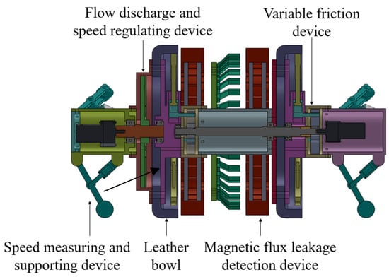
Figure 1.
Longitudinal cross-sectional schematic of the speed-controllable in-pipe MFL inspection robot.
2.2. Design of the Speed Measurement Support Mechanism
Common height adjustment methods for speed-measuring support devices include motor-lead screw adjustment, scissor-spring adjustment, slider-spring adjustment, and sleeve-spring adjustment (Figure 2). The motor-lead screw adjustment offers high support strength and a wide adjustment range but features a complex structure, requires power, and has high energy demands. The scissor-spring adjustment boasts high sensitivity yet has numerous rotating pairs in the scissor structure, resulting in low support strength. The slider-spring adjustment is sensitive and provides a certain level of support strength, but the slider mechanism requires guide rails and occupies a certain axial space. Compared with the previous three methods, the sleeve-spring adjustment combines the advantages of high sensitivity, simple structure, favorable support performance, and small space occupation. For these reasons, the sleeve-spring adjustment method is selected for the design of the speed measurement support device. As illustrated in Figure 3a,b, the speed measurement support mechanism employs a sleeve-spring adjustment method. In this configuration, a long support rod compresses the spring within the short rod sleeve to achieve wheel height variation. This approach offers advantages including highly responsive adjustment, structural simplicity, adequate load-bearing capacity, and compact spatial requirements.
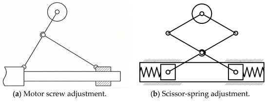
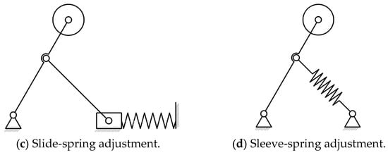
Figure 2.
Height adjustment mode of support device.
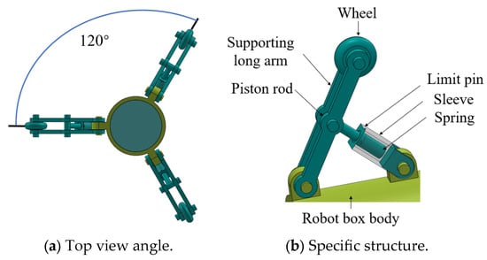
Figure 3.
Schematic diagram of the speed measurement support mechanism.
The pipeline inspection robot incorporates six sets of speed measurement support mechanisms. This configuration enables adaptation to minor pipeline diameter fluctuations and provides basic obstacle-crossing capability. Furthermore, multiple wheels transmit independent data streams, and their integration with speed sensors yields enhanced accuracy in velocity and positional measurements.
2.3. Design of the Flow-Discharge Speed Regulation Device
The flow-discharge valve is required to operate reliably under high-pressure natural gas conditions (up to 10 MPa) while providing continuous and controllable pressure relief for speed regulation. The key quantitative design requirements include the following: (i) a target adjustable torque range compatible with a compact electric motor; (ii) stable operation under inlet velocities of 15–30 m/s; (iii) sufficient safety margin against fluid impact and erosion; and (iv) geometric constraints imposed by the internal layout of motors, power supply, and sealing cups.
The MFL detection unit imposes specific speed requirements. Conventional practices in some contexts involve reducing in-pipe fluid velocity and flow rate to accommodate the inspection speed of the robot, but this approach severely impacts production efficiency. In contrast, the designed flow-discharge speed regulation device enables precise control of the operating speed of the robot with negligible fluid loss, rendering such losses insignificant.
The working principle of flow-discharge speed regulation involves modulating the discharge aperture area. This modulation alters the pressure differential acting on the robot and thereby regulates its velocity. Two primary valve structures are commonly employed in pipeline robots: the direct-acting conical orifice valve and the rotary disk valve.
As illustrated in Figure 4, the direct-acting conical orifice valve comprises four core components: a conical valve seat, a conical valve plug, a valve stem, and an actuator (typically a linear motor). The discharge flow rate is regulated by axially displacing the valve stem to adjust the gap distance between the valve plug and valve seat. This configuration offers advantages of structural simplicity and straightforward control. However, its operational limitations arise from the fluid impact pressure being directly borne by the valve plug, stem, and linear motor. Given the limited pressure tolerance of linear motors, exposure to high-pressure, high-flow fluid environments may cause premature failure. Additionally, this design exhibits moderate responsiveness.
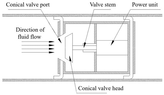
Figure 4.
Structural schematic diagram of the direct-acting conical discharge valve.
The rotary disk valve comprises an electric motor, a rotor disk, and a stationary valve cover. This valve regulates pressure and consequently adjusts speed by rotating the disk to modulate the aperture size of the discharge ports. As depicted in Figure 5, the motor is mounted on the housing and controls the rotation of the rotor disk, which maintains continuous contact with the stationary valve cover.
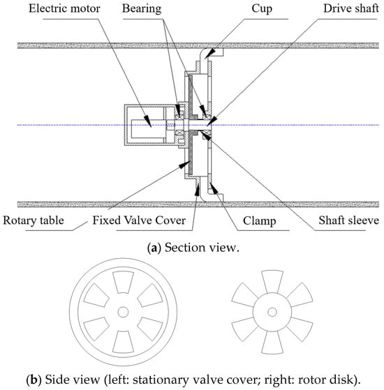
Figure 5.
Structural schematic diagram of the rotary disk discharge valve.
Both the size and geometry of the discharge apertures significantly influence flow regulation performance. After comprehensive evaluation, six equally spaced sector-shaped apertures were selected. Critically, the vanes of the rotor disk extend beyond the recesses of the stationary valve cover, optimizing force distribution across the vanes and enhancing their pressure-bearing capacity.
This configuration offers multiple advantages: structural simplicity, a compact spatial footprint, responsive control with minimal actuation, low energy consumption, and sufficient structural robustness to withstand fluid impact forces.
2.4. Design of the Magnetic Flux Leakage Detection Unit
The magnetic flux leakage (MFL) detection unit comprises two core subsystems: the sensor array and the magnetizing assembly, as schematically illustrated in Figure 6a. During pipeline traversal, the magnetizing assembly induces saturation magnetization in the pipe wall, while the sensor array detects resultant magnetic flux density. In defect-free regions (Figure 6b), magnetic flux remains uniformly distributed. Conversely, at defect locations (Figure 6c), flux leakage induces significant field perturbations. High-sensitivity detection elements detect and collect these signals, which are then transmitted to the control station. The control station, in accordance with the positioning data of the robot, marks the locations where magnetic flux fluctuations occur. It further calculates the severity of pipe wall damage based on the magnitude of such fluctuations, enabling the early implementation of measures to mitigate risks and thus accomplish the pipeline inspection process.
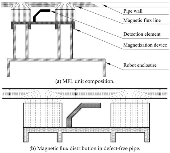
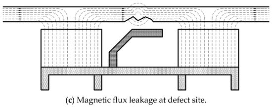
Figure 6.
Schematic diagram of the MFL detection unit.
2.5. Design of the Variable Friction Device
This paper proposed a mechanism capable of effectively regulating the frictional force between the cup seal and the pipeline inner wall, enabling both enhancement and reduction in the frictional force. As shown in Figure 7, spiral groove mechanism is designed, consisting of a spiral groove, a motor, and a pressure-regulating rod. The motor drives the spiral groove to rotate, thereby actuating the vertical movement of the transmission rod. The top of each transmission rod is equipped with a 90° arc-shaped end piece, which is fixedly connected to the cup seal. When the transmission rod moves upward, it compresses the cup seal to increase the frictional force; conversely, when the transmission rod moves downward, it pulls the cup seal to decrease the frictional force. The transmission rod is buffered by a spring to mitigate the impact force exerted on the pipeline. Compared with cam mechanisms, this mechanism features a relatively complex structure with more components. However, it offers notable advantages: the transmission rod allows for easy adjustment with a small rotation range. Furthermore, in contrast to cam mechanisms, the spiral groove mechanism can pull the cup seal toward the axis center, significantly improving the anti-jamming performance of the robot and preventing the robot from becoming stuck when passing through deformed pipeline sections. The design objective for the variable friction device is to provide a controllable friction adjustment range, one sufficient to overcome static jamming forces while simultaneously minimizing additional energy consumption and sealing cup wear.

Figure 7.
Schematic diagram of the helical groove mechanism.
3. Mechanical Performance Analysis of the In-Pipe MFL Inspection Robot
3.1. Kinematic Force Analysis of the Robot in Pipeline
The in-pipe robot advances via fluid-driven propulsion within a complex pipeline environment. Force analysis is essential to inform the design of the speed regulation mechanism of the robot. The force distribution during the pipeline traversal of the robot is illustrated in Figure 8.
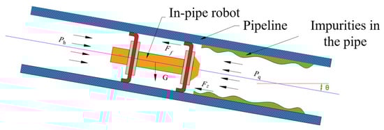
Figure 8.
Schematic diagram of in-pipe force analysis on the robot.
Based on force equilibrium principles, the following equation is derived from Figure 7:
where m is the net mass of the robot, g is the gravity acceleration,
vj is the velocity of the robot, Δp is the pressure differential of the fluid medium across the robot, A is the cross-sectional area subjected to the pressure differential is the gravitational acceleration, θ is the angle between the robot’s central axis and horizontal plane, Ff is the frictional force acting on the robot, and Fz is the resistance force from pipeline impurities.
The forces acting on the robot can be broadly categorized into two types: driving forces and resistance forces. Driving forces include the propulsion force provided by the fluid pressure differential across the robot and the gravitational driving force during downward pipe segments. Resistance forces include frictional forces acting on the robot, resistance from pipeline impurities, and the gravitational resistance during upward pipe segments.
3.2. The Driving Force of Robots
The robot experiences two primary driving forces during pipeline traversal: the gravitational driving force in downward pipe segments, and the propulsion force
generated by the fluid pressure differential across the robot, with the latter being the dominant driving force.
This differential manifests in two scenarios: a fully closed flow-discharge valve (Figure 9a) and a partially open valve (Figure 9b).
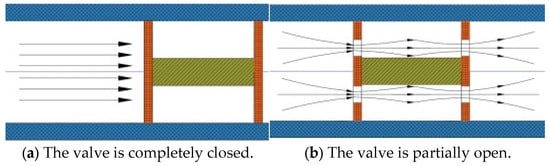
Figure 9.
Schematic diagram of in-pipe fluid flow.
The flow-discharge valve model involves fluid transitioning from large to small cross-sections and back, with critical pressure changes at the inlet, valve orifice, and outlet; Bernoulli’s equation governs this process:
where P1 is the pressure at the inlet, ρ is the density of fluid medium, v1 is the velocity at the inlet, P2 is the pressure at the outlet, v2 is the velocity at the outlet, ζ1 is the local pressure loss due to sudden contraction at the entrance, ζi is the frictional pressure loss within the valve orifice, which is negligible due to its minimal width, and ζ2 is the local pressure loss due to sudden expansion at the exit.
The localized pressure loss can be expressed as follows:
where ξ1 is the localized pressure loss coefficient for sudden fluid contraction, Ai is the cross-section of fluid within the valve orifice, A1 is the cross-section of fluid at the inlet, ξ2 is the localized pressure loss coefficient for sudden fluid expansion, and A2 is the cross-section of fluid at the outlet.
From flow rate continuity,
;
The driving force from the fluid pressure differential on the robot is
where Fd is the driving force exerted by fluid pressure differential on the robot, A′ is the thrust-applicable area, and A′ = A1 − Ai.
3.3. Resistance Calculation for the Robot
During pipeline traversal, the primary resistance forces acting on the robot include gravitational resistance during upward slopes. Frictional resistance from impurities (water, sediment, wax) is negligible. The frictional force
between the sealing cup and pipe wall is given by
where Ff is the total frictional force between sealing cup and pipe wall, μ is the friction coefficient, FG is the gravity-induced deformation force, FN1 is the interference fit force, and FN2 is the cantilever beam reaction force.
To quantify the gravitational effects on friction, a differential force analysis is applied to the sealing cup. The cup is divided into infinitesimal sectors with angle dφ, and the gravitational force on a sector is
where dG is the gravitational force on an infinitesimal sector, G is the total robot weight, r is the sealing cup radius, and dφ is the angular span of infinitesimal sector.
As shown in Figure 10, the normal reaction force on a sector is
where dFG is the normal reaction force on an infinitesimal sector.
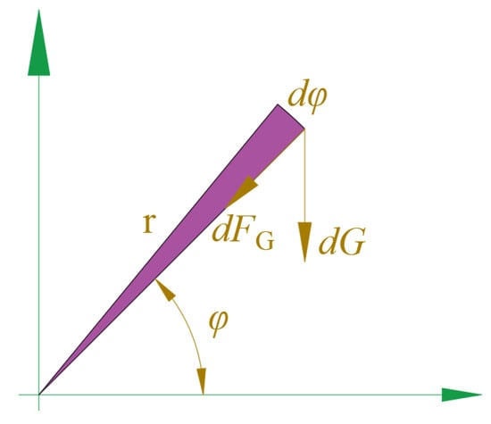
Figure 10.
Force analysis of an infinitesimal sector.
When FG = 0, it indicates that gravity neither increases nor decreases the frictional force of the robot. Gravity increases deformation at the bottom of the sealing cup while reducing deformation at the top, resulting in mutually counteracted effects on friction. However, this asymmetric deformation causes accelerated wear at the lower section of the cup. To mitigate the influence of gravity, the speed measurement support mechanism equalizes force distribution across the sealing cup (Figure 11). Friction from the support wheels is rolling friction, which is orders of magnitude smaller than the sliding friction under equivalent normal forces and thus negligible.

Figure 11.
Schematic diagram of pipeline reaction forces on the robot under gravitational effects.
3.4. Parameter Calculation of the Sealing Cup
To enable fluid-driven motion within the pipeline, the sealing cup employs an interference fit with the pipe wall and is constructed from rigid material. A deformation mechanics model is established for the sealing cup, comprising two sub-models:
- (1)
- Cylindrical Interference Mechanics Model: The lip region of the sealing cup experiences contact pressure FN1, inducing compressive stress σN1. As shown in Figure 12, to determine FN1, the force model is converted by equating lip pressure to an externally applied compressive stress σN1 causing a reduction in the outer diameter of the cup.
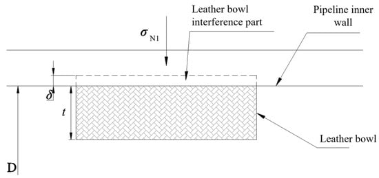 Figure 12. Schematic diagram of the cylindrical interference mechanics model.
The deformation of the sealing cup under external force is calculated as follows:
where δ is the deformation of the sealing cup under compressive force, D is the inner diameter of the pipe wall, E is the elastic modulus of the cup material, t is the thickness of the sealing cup, and σN1 is the compressive stress on the sealing cup.
Rearranging Equation (9) yields the compressive stress:
where υ is the Poisson’s ratio of the cup material.
- (2)
- Cantilever Beam Mechanics Model: Under pressure FN2, the sealing cup experiences compressive stress σN2. The force diagram is shown in Figure 13.

Figure 13.
Schematic diagram of the mechanical model of a cantilever beam under pressure FN2.
The deflection equation of the cantilever beam is as followed:
where ω is the cantilever beam deflection, M(x) is the bending moment, Iz is the moment of inertia, FS is the pressure per unit cup segment, L is the length of the inclined cup segment, α is the inclination angle of the cup, dβ is the angular span of an infinitesimal sector, and b is the axial contact length. Substituting Equation (14) into Equation (11),
Deformation due to compressive stress σN2:
Cantilever beam stress:
Combining Equations (10) and (17), the total stress on the cup is as follows:
The force from the interference fit is as follows:
where S is the contact area between the cup and pipe wall.
where i is the number of sealing cups installed.
The total frictional force is
The sealing cup for fluid-driven pipeline robots is typically fabricated from polyurethane rubber, a material exhibiting high contact strength, superior elasticity, wear resistance, and minimal permanent deformation. It also benefits from mature manufacturing processes and broad industrial applications. The robot employs polyurethane rubber with an elastic modulus E of 350 MPa and Poisson’s ratio ν of 0.47 for the sealing cups. Designed primarily for pipelines with diameter D of 610 mm, the friction coefficient μ between the cup and pipe wall is 0.2. The axial length of the inclined cup segment is 50 mm: Lsinα = 50 mm.
When the cup thickness t is 30 mm and the axial contact length b is 60 mm, Equation (23) indicates a linear relationship between the cup interference ratio δ and the total frictional force
Based on practical engineering applications, a 3% interference ratio is adopted. With δ = 3% and t = 30 mm, Equation (23) reveals a linear correlation between the axial contact length *b* and
Considering operational longevity and space allocation for the pressure-regulating rod in the variable friction device, the contact length is selected as b ≥ 20 mm. Under δ = 3% and b = 20 mm, Equation (23) demonstrates the exponential growth of
with increasing cup thickness t, as shown in Figure 14. In this study, the optimal sealing cup thickness is defined by a trade-off objective function that balances sealing reliability and friction-induced motion resistance. Increasing the thickness enhances sealing performance but leads to a rapid rise in frictional force. As shown in Figure 14, a thickness of 30 mm provides sufficient sealing capability while maintaining friction within an acceptable range, and is therefore selected as the optimal design value under this objective.
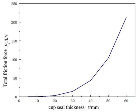
Figure 14.
Relationship between sealing cup thickness t and total frictional force.
With sealing cup thickness t = 30 mm, axial contact length b = 20 mm, interference ratio δ = 3%, and inclined segment length L = 70 mm, Equation (23) indicates a negative exponential correlation between the total frictional force
and both the cup inclination angle α and inclined segment length L, as shown in Figure 15 and Figure 16. To maintain adequate taper while minimizing friction, the inclination angle is selected as 55°.
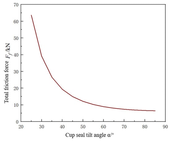
Figure 15.
Relationship between sealing cup inclination angle and total frictional force.
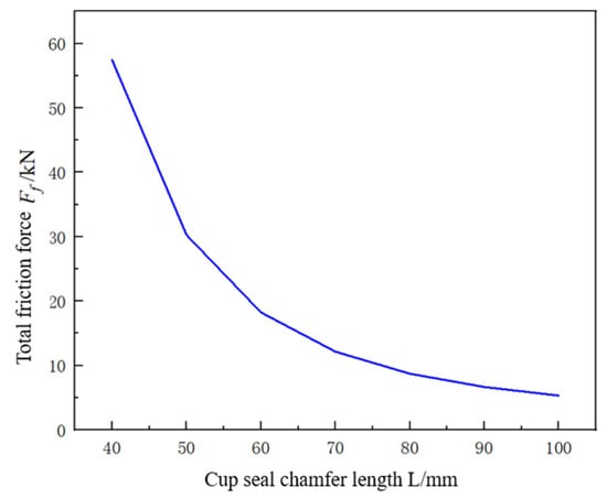
Figure 16.
Relationship between inclined segment length and total frictional force.
Based on the above analysis, the sealing cup design parameters are finalized in Table 1.

Table 1.
Sealing cup design parameters.
4. Simulation and Experimental Analysis of the In-Pipe MFL Inspection Robot
Analyze the motion of the robot in-pipe fluid and simulate the real physical environment as closely as possible. While ensuring computational accuracy and grid quality, minimize the number of grids and save computation time. HyperMesh 2022 is used for the mixed partitioning of structural and non-structural grids. Irregular fluids are partitioned into non-structural grids to ensure their partitioning accuracy. Fluid parts with regular shapes are partitioned into structural grids, while important parts with small sizes and complex structures are encrypted and verified for grid independence. The partitioned grids are shown in Figure 17. Fluid simulations were conducted with natural gas (density: 0.8 kg/m3, viscosity: 0.012 mPa·s) using the k-ε realizable turbulence model and enhanced wall treatment. Boundary conditions included velocity inlets (15 m/s, 20 m/s, 25 m/s) and a pressure outlet (10 MPa). Models with different discharge areas are tested by adjusting orifice sizes, with pressure differentials recorded. The near-wall resolution was evaluated using the non-dimensional wall distance y+, which was maintained within the recommended range for the enhanced wall treatment approach. As shown in Table 2, when the number of grids is 3,154,600, the fluid pressure difference before and after the robot remains stable, indicating that the sensitivity of numerical results to grid size has significantly decreased, and the calculation results no longer change significantly with further grid refinement, meeting the requirement of grid independence.
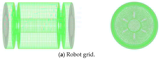
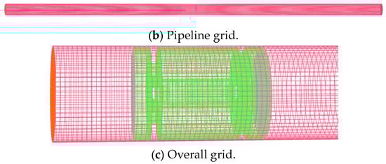
Figure 17.
Grid division of the in-pipe mfl inspection robot.
Table 2.
Fluid pressure difference between front and back under different mesh counts.
The experiment validates the speed regulation efficacy and anti-jamming mechanism rationality while comparing results with simulations.
A scaled-down robot model used air as the driving fluid for safety. The simplified model (Figure 18) retained valve opening control and simulated friction adjustment via clamping plates compressing seals. The acrylic test pipe (ID: 50 mm, length: 2 m) ensured visibility. A gas compression pump supplied pressurized fluid; high-speed cameras recorded positional data for velocity calculation.
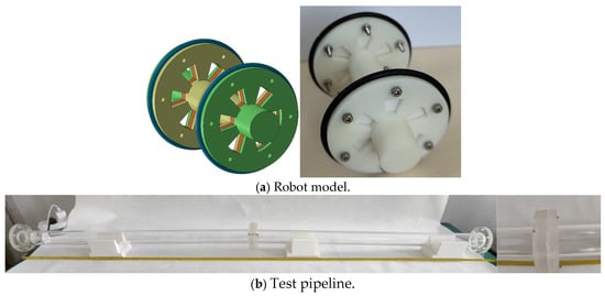
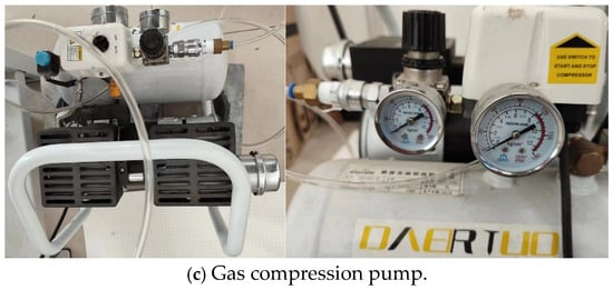
Figure 18.
Experimental model of the in-pipe MFL inspection robot.
4.1. Determination of Discharge Area for the Flow-Discharge Speed Regulation Device
The velocity contour (Figure 19a) shows flow acceleration at the discharge orifice followed by gradual stabilization, aligning with flow continuity; the pressure contour (Figure 19b) confirms a higher pressure behind the robot versus lower pressure ahead, with orifices enabling pressure relief to generate the driving differential; velocity streamlines (Figure 19c) visualize flow paths.

Figure 19.
Simulation results of flow-discharge regulation (25 m/s, discharge area ratio 0.17).
The relationship between the discharge area ratio of the robot model and the fluid pressure differential is shown in Figure 20. With constant inlet velocity and outlet pressure, the pressure differential decreases as the discharge area ratio increases, while the rate of change gradually diminishes. When the discharge area ratio exceeds 20%, the pressure differential variation significantly diminishes. Given the spatial requirements for internal components and edge sealing cups, the optimal discharge area is selected as 30%.
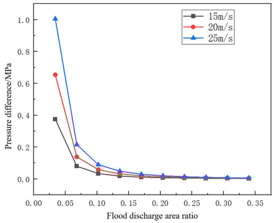
Figure 20.
Relationship between discharge area ratio and pressure differential at different inlet velocities (15, 20, 25 m/s).
4.2. Valve Opening Degree vs. Valve Torque
To obtain valve torque under high-pressure/high-flow conditions, simulations used a 30 m/s inlet velocity and 10 MPa outlet pressure. Models with varying valve openings monitored torque in the rotating fluid domain. The velocity streamline plot and pressure contour plot from the model simulation (for a 90% opening example) are shown in Figure 21.
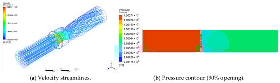
Figure 21.
Flow contours in pipeline.
Figure 22 shows the relationship between the valve opening and torque. Torque decreases with increasing opening. At 10% opening, torque is 69 MPa; a turning point occurs at 30% opening. Beyond 30%, the curve’s slope decreases. Within the 10–90% operational range, torque varies between 20 and 69 MPa.

Figure 22.
Valve opening vs. torque.
4.3. Fluid Velocity vs. Valve Torque
Inlet velocity also affects torque. With the valve opening fixed at 30%, varying inflow velocities yielded torque data (Figure 23). Torque increases linearly with fluid velocity, enabling the calculation of valve-closing torque.
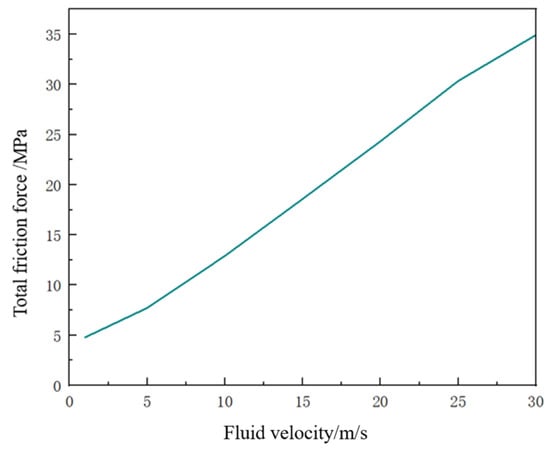
Figure 23.
Fluid velocity vs. torque.
4.4. Speed Regulation Performance of Variable Friction Device
When hitting obstacles while moving, conventional pipeline robots usually close the drainage valve to boost rear fluid pressure, overcoming tangential resistance from welds on the sealing cup. While this method can mitigate general blockages, excessive resistance may not only hinder effective robot propulsion but also potentially cause damage to the robot body and the cup due to excessively high shear stress.
The variable friction device offers a more effective solution to address robot blockages. This device applies radial tension to the cup via a pressure-adjusting rod, causing the outer diameter of the cup to contract. Consequently, weld shear force turns to lower frictional resistance, cutting or eliminating blockages. Moreover, when the pipeline diameter exceeds the compressed size of the cup, the device prevents the robot from becoming trapped. Its diameter-adjusting feature helps the robot pass smoothly through sudden diameter drops.
Prolonged friction-based deceleration accelerates cup wear and energy consumption. Thus, a coordinated strategy is implemented: (a) High-speed deceleration: First engage the variable friction device to rapidly increase friction, and then activate the flow-discharge device to reduce fluid pressure differential. Gradually decrease friction as pressure stabilizes. (b) Low-speed acceleration: First reduce friction via the variable friction device, and then increase fluid pressure differential via the flow-discharge device. Gradually decrease friction until stable speed. (c) Speed fluctuations: Prioritize rapid adjustment with the variable friction device, and then stabilize with the flow-discharge device.
Three simulation groups validate efficacy: Group 1 (flow-discharge only: increased valve opening), Group 2 (variable friction only: increased friction), Group 3 (coordinated control: increased opening + friction). All models shared identical initial speeds; regulation initiated at t = 1 s. Speed curves (Figure 24) show rapid deceleration (steepened slope) post-intervention, moderating as speed decreases, culminating in a new steady state. Stabilization times were as follows: Group 1 (~1.5 s), Group 2 (~0.8 s), Group 3 (~0.5 s). Coordinated control reduces regulation time by ~66.7% versus flow-discharge alone.

Figure 24.
Speed profile.
Acceleration strategies mirror deceleration (reducing friction/opening), with analogous time advantages. Per Equation (6), friction depends on pipe coefficients: static friction (0.3) and dynamic friction (0.2). During jamming, static friction necessitates gas compression to provide the breakthrough force, causing speed overshoot. Newtonian analysis (Figure 25) indicates the following: Group 1 exhibits post-breakthrough speed surge and overshoot due to pressure hysteresis; Group 2 minimizes fluctuations by avoiding gas compression; Group 3 reduces speed fluctuations by ~37% versus Group 1.
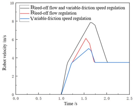
Figure 25.
Speed fluctuation comparison.
4.5. Experimental Results Analysis
Figure 26 shows the robot traversing the pipeline.
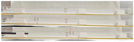

Figure 26.
Operational process of the robot.
A parallel ruler recorded the transit times at marked positions. Clamping pressure adjustments tested seal deformation impact on anti-jamming performance; valve opening variations measured speed response. Paper inserts simulated the pipe diameter reductions (Figure 27): larger seal diameters failed to pass constrictions (Figure 27a), while reduced diameters succeeded (Figure 27b), confirming the anti-jamming enhancement.
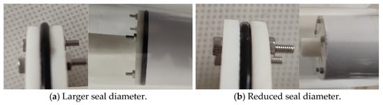
Figure 27.
Anti-jamming performance test.
Valve openings (10%, 20%, 30%) were tested under identical conditions. Table 3 records the transit times at marked sections:
Table 3.
Transit times at marked sections/s.
The calculated average velocities (Figure 28) confirm the inverse correlation between the valve opening and speed, demonstrating effective speed control.
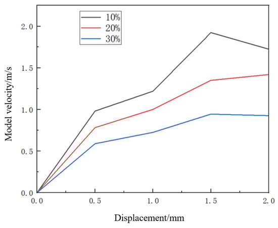
Figure 28.
Operational velocities.
As shown in Table 4, compared with the existing speed-controllable pipeline robots reported in [2,9,11,12,13], the proposed system demonstrates a comparable or shorter speed regulation time while requiring no external braking devices. In addition, the coordinated use of variable friction and flow-discharge regulation provides enhanced anti-jamming capability under high-pressure conditions.
Table 4.
Performance summary table.
Despite its advantages, the proposed mechanism has several limitations. The long-term durability of the sealing cup under high-pressure operation requires further investigation, particularly regarding wear and aging. In addition, motor energy consumption and performance under contaminated or sediment-laden pipelines were not addressed in this study and will be considered in future work.
5. Conclusions
This study designed and analyzed a novel variable friction in-pipe magnetic flux leakage (MFL) detection robot for long-distance natural gas pipeline inspection. Through systematic mechanical modeling, simulation analysis, and experimental validation, the main conclusions are as follows:
- (1)
- The feasibility of the integrated design has been validated: A prototype featuring a synergistic control system integrating a rotary disk valve-type flow-discharge speed regulation device and a helical groove-driven variable friction device was successfully developed. Experiments demonstrated that this dual-mechanism system can effectively regulate the speed of the robot (achieving a speed adjustment range of approximately ±40% of the initial speed by varying the valve opening) and enable rapid stabilization (the coordinated strategy reduced the regulation time by about 66.7% compared to using the valve alone) under low-pressure gas drive conditions.
- (2)
- Key design parameters were quantified and determined: Based on the established mechanical model of the sealing cup, the quantitative relationship between the frictional force and structural parameters was clarified. By balancing the sealing reliability against frictional resistance, an optimal thickness of 30 mm was determined. Furthermore, integrating fluid simulation results with internal spatial constraints led to an optimized discharge area ratio of 30%, providing a concrete basis for engineering implementation.
- (3)
- Anti-jamming performance was supported by both mechanism analysis and experiments: The variable friction device provides a “soft-pass” capability against sudden pipeline diameter changes by actively retracting the sealing cup radially. Scaled-model experiments visually verified the effectiveness of this function, demonstrating that proactively reducing the seal diameter can effectively prevent jamming when encountering simulated local protrusions.
Author Contributions
Conceptualization, H.L. and Y.L.; Methodology, H.L., S.Y. and Y.L.; Software, D.C. and S.Y.; Formal analysis, J.L.; Investigation, D.C., S.Y., J.L. and Y.L.; Resources, Y.L.; Data curation, D.C., S.Y., J.L. and Y.L.; Writing—original draft, H.L., S.Y., J.L. and Y.L.; Writing—review & editing, H.L., J.L. and Y.L. All authors have read and agreed to the published version of the manuscript.
Funding
This research was funded by National Natural Science Foundation of China, 52301377; China Postdoctoral Science Foundation, 2024M753616 and Science Foundation of China University of Petroleum, Beijing, 2462025XKBH002.
Data Availability Statement
The original contributions presented in this study are included in the article. Further inquiries can be directed to the corresponding author.
Conflicts of Interest
Author Haichao Liu and author Shining Yuan were employed by CNOOC (Tianjin) Pipeline Engineering Technology Co., Ltd., author Dongliang Cao was employed by Changqing Oilfield (Yulin) Oil and Gas Co., Ltd. The remaining authors declare that the research was conducted in the absence of any commercial or financial relationships that could be construed as a potential conflict of interest.
Glossary, Scheme and Nomenclature
| Abbreviation | Full Term | Description |
| MFL | Magnetic Flux Leakage | Non-destructive testing method based on magnetic flux leakage |
| PIG | Pipeline Inspection Gauge | Device used for pipeline inspection and maintenance |
| CFD | Computational Fluid Dynamics | Numerical simulation of fluid flow |
| GMR | Giant Magneto-Resistance | High-sensitivity magnetic sensing technology |
| CNN | Convolutional Neural Network | Deep learning model for feature extraction |
| RL | Reinforcement Learning | Machine learning method based on reward mechanisms |
| PSO | Particle Swarm Optimization | Swarm intelligence optimization algorithm |
| SVM | Support Vector Machine | Supervised learning model for classification |
| SSA | Sparrow Search Algorithm | Swarm intelligence optimization algorithm |
| Symbols | Description | |
| m | net mass of the robot | |
| g | gravity acceleration | |
| Δp | pressure differential of the fluid medium across the robot | |
| A | cross-sectional area | |
| Ff | frictional force acting on the robot | |
| θ | angle between the robot’s central axis and horizontal plane | |
| Fz | resistance force from pipeline impurities | |
| P1 | pressure at inlet | |
| P2 | pressure at outlet | |
| v1 | velocity at inlet | |
| v2 | velocity at outlet | |
| ζ1 | local pressure loss due to sudden contraction at entrance | |
| ζi | frictional pressure loss | |
| ζ2 | local pressure loss due to sudden expansion at exit | |
| ξ1 | localized pressure loss coefficient for sudden fluid contraction | |
| ξ2 | localized pressure loss coefficient for sudden fluid expansion | |
| Ai | cross-section of fluid within the valve orifice | |
| A1 | cross-section of fluid at inlet | |
| A2 | cross-section of fluid at outlet | |
| Fd | driving force exerted by fluid pressure differential on the robot | |
| A′ | thrust-applicable area | |
| Ff | total frictional force between sealing cup and pipe wall | |
| μ | friction coefficient | |
| FG | gravity-induced deformation force | |
| FN1 | interference fit force | |
| FN2 | cantilever beam reaction force | |
| dG | gravitational force on an infinitesimal sector | |
| G | total robot weight | |
| r | sealing cup radius | |
| dφ | angular span of infinitesimal sector | |
| dFG | normal reaction force on an infinitesimal sector | |
| δ | deformation of the sealing cup under compressive force | |
| D | inner diameter of the pipe wall | |
| E | elastic modulus of the cup material | |
| t | thickness of the sealing cup | |
| σN1 | compressive stress on the sealing cup | |
| ω | cantilever beam deflection | |
| M(x) | bending moment | |
| Iz | moment of inertia | |
| FS | pressure per unit cup segment | |
| L | length of the inclined cup segment | |
| α | inclination angle of the cup | |
| dβ | angular span of an infinitesimal sector | |
| b | axial contact length | |
| S | contact area between cup and pipe wall | |
| i | number of sealing cups installed | |
References
- Nguyen, H.-H.; Park, J.-H.; Jeong, H.-Y. A Simultaneous Pipe-Attribute and PIG-Pose Estimation (SPPE) Using 3-D Point Cloud in Compressible Gas Pipelines. Sensors 2023, 23, 1196. [Google Scholar] [CrossRef] [PubMed]
- Wang, Y.; Wang, J.; Zhou, Q.; Feng, S.; Wang, X. Mechanism design and mechanical analysis of pipeline inspection robot. Ind. Robot.-Int. J. Robot. Res. Appl. 2025, 52, 137–143. [Google Scholar] [CrossRef]
- Tang, C.; Du, B.; Jiang, S.; Shao, Q.; Dong, X.; Liu, X.-J.; Zhao, H. A pipeline inspection robot for navigating tubular environments in the sub-centimeter scale. Sci. Robot. 2022, 7, eabm8597. [Google Scholar] [CrossRef] [PubMed]
- Li, H.; Li, R.; Zhang, J.; Zhang, P. Development of a Pipeline Inspection Robot for the Standard Oil Pipeline of China National Petroleum Corporation. Appl. Sci. 2020, 10, 2853. [Google Scholar] [CrossRef]
- Kakogawa, A.; Ma, S. Design of a multilink-articulated wheeled pipeline inspection robot using only passive elastic joints. Adv. Robot. 2018, 32, 37–50. [Google Scholar] [CrossRef]
- Guo, Z.; Liu, Y.; Zhou, F.; Zhang, P.; Song, Z.; Tan, H. Design of hexapod robot equipped with omnidirectional vision sensor for defect inspection of pipeline’s inner surface. Meas. Sci. Technol. 2024, 35, 115901. [Google Scholar] [CrossRef]
- Yin, J.; Liu, X.; Wang, Y.; Wang, Y. Design and motion mechanism analysis of screw-driven in-pipe inspection robot based on novel adapting mechanism. Robotica 2024, 42, 1297–1319. [Google Scholar] [CrossRef]
- Elankavi, R.S.; Dinakaran, D.; Doss, A.S.A.; Chetty, R.M.K.; Ramya, M.M. Design of a wheeled-type In-Pipe Inspection Robot to overcome motion singularity in curved pipes. J. Ambient. Intell. Smart Environ. 2023, 16, 43–55. [Google Scholar] [CrossRef]
- Ma, Q.; Yang, Z.; Yue, C.; Liu, S. Investigation on mechanical behaviour of underwater launching process of bidirectional pigging robot in the subsea oil pipeline using Coupled Eulerian-Lagrangian method. Proc. Inst. Mech. Eng. Part M-J. Eng. Marit. Environ. 2024, 238, 847–864. [Google Scholar] [CrossRef]
- Venkateswaran, S.; Chablat, D. Stability analysis of tensegrity mechanism coupled with a bio-inspired piping inspection robot. arXiv 2022, arXiv:2206.01433. [Google Scholar] [CrossRef]
- Jeon, K.-W.; Jung, E.-J.; Bae, J.-H.; Park, S.-H.; Kim, J.-J.; Chung, G.; Chung, H.-J.; Yi, H. Development of an In-Pipe Inspection Robot for Large-Diameter Water Pipes. Sensors 2024, 24, 3470. [Google Scholar] [CrossRef]
- Jang, M.-W.; Lee, J.-Y.; Jeong, M.-S.; Hong, S.-H.; Shin, D.-H.; Seo, K.-H.; Suh, J.-H. Development of Spiral Driving Type Pipe Inspection Robot System for Magnetic Flux Leakage. J. Korean Soc. Precis. Eng. 2022, 39, 603–613. [Google Scholar] [CrossRef]
- Kim, H.M.; Yoo, H.R.; Park, G.S. A New Design of MFL Sensors for Self-Driving NDT Robot to Avoid Getting Stuck in Curved Underground Pipelines. IEEE Trans. Magn. 2018, 54, 1–5. [Google Scholar] [CrossRef]
- Wang, R.; Kawamura, Y. An Automated Sensing System for Steel Bridge Inspection Using GMR Sensor Array and Magnetic Wheels of Climbing Robot. J. Sens. 2016, 2016, 8121678. [Google Scholar] [CrossRef]
- Kim, J.-W.; Choi, J.-S.; Lee, E.-C.; Park, S.-H. Field Application of a Cable NDT System for Cable-Stayed Bridge Using MFL Sensors Integrated Climbing Robot. J. Korean Soc. Nondestruct. Test. 2014, 34, 60–67. [Google Scholar] [CrossRef]
- Lynch, A.J. Magnetic Flux Leakage Robotic Pipe Inspection: Internal and External Methods. Master’s Thesis, Rice University, Houston, TX, USA, 2009. [Google Scholar]
- Pan, J.; Gao, L. A novel method for defects marking and classifying in MFL inspection of pipeline. Int. J. Press. Vessel. Pip. 2023, 202, 104892. [Google Scholar] [CrossRef]
- Feng, J.; Zhang, X.; Lu, S.; Yang, F. A Single-Stage Enhancement-Identification Framework for Pipeline MFL Inspection. IEEE Trans. Instrum. Meas. 2022, 71, 1–13. [Google Scholar] [CrossRef]
- Wu, Z.; Deng, Y.; Liu, J.; Wang, L. A Reinforcement Learning-Based Reconstruction Method for Complex Defect Profiles in MFL Inspection. IEEE Trans. Instrum. Meas. 2021, 70, 1–10. [Google Scholar] [CrossRef]
- Chen, J.; Kang, X.; Zhang, X.; He, R.; Meng, T.; Song, K. A novel identification approach for corrosion and gouging of oil and gas pipelines based on low magnetisation level MFL inspection. Insight 2022, 64, 270–278. [Google Scholar] [CrossRef]
- Shi, P.; Zhang, P.; Hao, S.; Wang, W.; Gou, X. Classification and evaluation for nearside/backside defect via magnetic flux leakage: A dual probe design with SVM and PSO intelligence algorithms. NDT E Int. 2024, 144, 103100. [Google Scholar] [CrossRef]
- Shen, Y.; Zhou, W. Development of a convolutional neural network model to predict the size and location of corrosion defects on pipelines based on magnetic flux leakage signals. Int. J. Press. Vessel. Pip. 2024, 207, 105123. [Google Scholar] [CrossRef]
Disclaimer/Publisher’s Note: The statements, opinions and data contained in all publications are solely those of the individual author(s) and contributor(s) and not of MDPI and/or the editor(s). MDPI and/or the editor(s) disclaim responsibility for any injury to people or property resulting from any ideas, methods, instructions or products referred to in the content. |
© 2026 by the authors. Licensee MDPI, Basel, Switzerland. This article is an open access article distributed under the terms and conditions of the Creative Commons Attribution (CC BY) license.