Kinematics of the Milky Way from the Statistical Analysis of the Gaia Data Release 3

Abstract

The aim of the analysis of data from the Gaia Space Observatory is to obtain kinematic parameters of the collective motion of stars in a part of our galaxy. This research is based on a statistical analysis of the motion of $55,038,539$ stars selected in different directions from the Sun up to a distance of 3–6 kpc. We developed statistical methods for the analysis working with input data represented by the full astrometric solution (five parameters). Using the proposed statistical methods, we obtained the local velocity of the Sun $\left(U_{\odot },V_{\odot },W_{\odot }\right)=(9.58,16.25,7.33)\pm {(0.05,0.04,0.02)}_{stat}\pm {(0.7,0.9,0.1)}_{syst}$ km/s and the rotation velocity of the galaxy at different radii. For the Sun’s orbit radius, we obtained the velocity of the galaxy rotation$V_c\approx 234\pm 4$ km/s. Collective rotation slows down in the region under study linearly with distance from the disk plane: $\Delta V/\Delta Z\cong 33.5\mathrm{km}{\mathrm{s}}^{-1}{\mathrm{kpc}}^{-1}$. We showed that the different kinematic characteristics and distributions, which depend on the position in the galaxy, can be well described in the studied 3D region by a simple Monte Carlo simulation model, representing an axisymmetric approximation of the galaxy kinematics. The optimal values of the six free parameters were tuned by comparison with the data.

1. Introduction

Our galaxy, the Milky Way (MW), is a unique laboratory for gravity research and for understanding the formation and evolution of galaxies. In recent years, the Gaia Space Observatory has acquired a huge amount of precise astrometric, photometric, and spectroscopic data on stars in the MW [1]. The analysis of these data has been the subject of many thousands of publications.

The Gaia DR3 catalogue provides very rich input data for creating a kinematic map of the MW, much more detailed than previously possible. In general, it encompasses various structures on different scales, from the orbiting of small gravitationally bound systems, binaries, and multiple-bound systems [2] to the streaming motions of stellar fields in spiral arms [3,4] with various turbulences and fluctuations and to the collective rotation of the whole galactic disk with the galactic halo.

The nature of the rotation suggests the presence of dark matter, which generates a substantial part of the MW mass, see [5,6,7,8,9,10,11,12,13,14] and the overview [15]. Recent studies of MW kinematics have shown accurate results on the MW rotation represented by the rotation curve (RC) defined as the dependence of the orbital velocity on the radius. These curves are the basic input for models accounting for the presence of dark matter. This is why these two topics often appear together in papers.

Along with gravity, the formation and evolution of the stars themselves are also controlled by the forces of the microworld (strong, electroweak—unified electromagnetic+weak) based on a well-verified standard model. The nature and origin of dark matter at the microscopic level have not yet been explained.

Very important topics concern the detailed mapping of many kinematic substructures beyond axial symmetry [16,17,18,19,20,21,22,23,24,25]. An overview of the integrated, structural, and kinematic parameters of the galaxy is given in [26].

The first goal of our study is to use statistical methods to determine the local velocity of the Sun and to analyse the collective orbital motion of stars in the galactic plane and beyond. Because the methods used do not require knowledge of radial velocities, we can access larger samples of stars [27,28]. The second goal is to obtain the 3D axisymmetric approximation of the kinematic MW image generated by averaging local asymmetric substructures. This image can be useful in determining the scale of local asymmetries or as input for validating axisymmetric models.

In Section 2, we describe our methodology and define the basic concepts and quantities we will work with. First, we define transformation relations between galactic and Galactocentric reference frames. The first system is used to acquire and present Gaia data, while the second is suitable for simulation and data interpretation. Then, the definition of the axisymmetric Monte Carlo model in the Galactocentric reference frame follows. The model is based on a triple (partially asymmetric) Gaussian distribution, which depends on the distance from the galactic plane and is defined by six free parameters. Next, we define the sky sectors to be analysed and the cuts for selecting accurate data. In Section 3, we present our methods together with the results obtained from velocity distributions in the different sectors of the sky. Analyses of these distributions provide precise results concerning the local and orbital velocity of the Sun (Section 3.1), the different RC representations (Section 3.2), and the setting of the free parameters of the simulation model (Section 3.3). This is followed by a comparison of the simulation with all relevant distributions (Section 3.4). The obtained results and their agreement with the simulation model are discussed in more detail in Section 4. The discussion includes a comparison of the results obtained with other available data.

2. Methodology and Definitions

2.1. Reference Frames

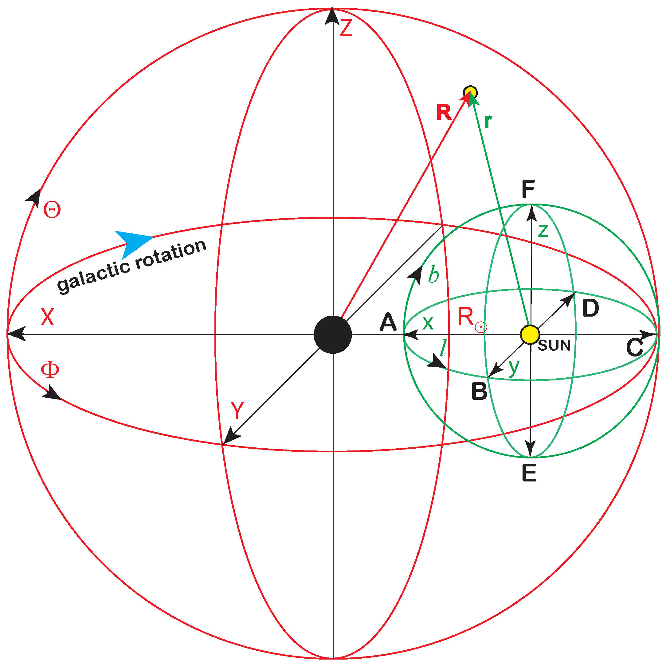
Positions of sources in Gaia data are represented in angular galactic coordinates: longitude (l) and latitude (b). Using parallax, we can also define the distance r of the source from the Sun. For our analysis, representation in Galactocentric coordinates will also be important. The relation between both reference frames is illustrated in Figure 1. The axes of the galactic and Galactocentric reference frames are defined as

$$\begin{array}{cc}\hfill x& =rcoslcosb,y=rsinlcosb,z=rsinb,\hfill \\ \hfill X& =Rcos\mathrm{\Phi }cos\mathrm{\Theta },Y=Rsin\mathrm{\Phi }cos\mathrm{\Theta },Z=Rsin\mathrm{\Theta }.\hfill \end{array}$$

(1)

For clarity, we will use the following convention throughout the paper: positions, velocities, and their coordinates are denoted in lowercase (uppercase) in the galactic (Galactocentric) reference frame. So, the direction x points to the centre of the galaxy and the direction y is the direction of the MW rotation. The corresponding coordinates are related as

$$X=x-R_{\odot };Y=y;Z=z.$$

(2)

Radius $R_{\odot }$ represents the distance of the Sun from the galactic centre. The values obtained in the measurements are in the interval 7.1–8.92 kpc [26]. For our analysis, we used the recent value $R_{\odot }\approx 8.178$ kpc [29]. The small parameter $Z_{\odot }\approx 0.0208$ kpc [30] defining the position of the Sun above the galactic plane is neglected in our analysis. The validity of this approximation will be commented on in Section 3.3.

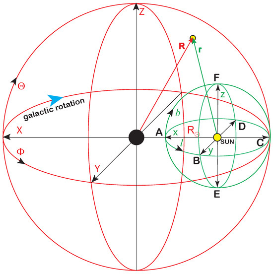
Figure 1. Galactic (green) and Galactocentric (red) reference frames. The letters A–F indicate the directions of the primary sectors of our analysis, see Table 1.

Then, the transformation between spherical coordinates $\left(r,l,b\right)\to \left(R,\mathrm{\Phi },\mathrm{\Theta }\right)$ of both the frames is defined by equations

$$\begin{array}{cc}\hfill R& =\sqrt{r^2+R_{\odot }^2-2R_{\odot }x},\mathrm{\Theta }=arcsin{\displaystyle \frac{z}{R}},\hfill \\ \hfill \mathrm{\Phi }\left(x>R_{\odot }\right)& =arcsin{\displaystyle \frac{y}{Rcos\mathrm{\Theta }}},\mathrm{\Phi }\left(x\le R_{\odot }\right)=\pi -arcsin{\displaystyle \frac{y}{Rcos\mathrm{\Theta }}}\hfill \end{array}$$

(3)

and inversely $\left(R,\mathrm{\Phi },\mathrm{\Theta }\right)\to$$\left(r,l,b\right):$

$$\begin{array}{cc}\hfill r& =\sqrt{R^2+R_{\odot }^2+2R_{\odot }X},b=arcsin{\displaystyle \frac{Z}{r}}\hfill \\ \hfill l\left(X>R_{\odot }\right)& =\pi -arcsin{\displaystyle \frac{Y}{rcosb}},l\left(X\le R_{\odot }\right)=arcsin{\displaystyle \frac{Y}{rcosb}},\hfill \end{array}$$

(4)

where $x,y,z,X,Y,Z$ are defined by (1). We will need these transformations to model and simulate the motion of the stars in Section 2.2 and Section 3.4. The spherical coordinates $\left(R,\mathrm{\Phi },\mathrm{\Theta }\right)$ are simply related to the cylindrical coordinates $\left(R_c,\mathrm{\Phi },Z\right)$:

$$R_c=Rcos\mathrm{\Theta };Z=Rsin\mathrm{\Theta }.$$

(5)

Next, we will need vectors forming the local orthonormal bases in both reference frames:

$$\begin{array}{c}\hfill {\mathbf{N}}_{\mathrm{\Phi }}=\left(-sin\mathrm{\Phi },cos\mathrm{\Phi },0\right),{\mathbf{N}}_{\mathrm{\Theta }}=\left(-cos\mathrm{\Phi }sin\mathrm{\Theta },-sin\mathrm{\Phi }sin\mathrm{\Theta },cos\mathrm{\Theta }\right),\\ \hfill {\mathbf{N}}_R=\left(cos\mathrm{\Phi }cos\mathrm{\Theta },sin\mathrm{\Phi }cos\mathrm{\Theta },sin\mathrm{\Theta }\right),\end{array}$$

(6)

$$\begin{array}{c}\hfill {\mathbf{n}}_l=\left(-sinl,cosl,0\right),{\mathbf{n}}_b=\left(-coslsinb,-sinlsinb,cosb\right),\\ \hfill {\mathbf{n}}_r=\left(-coslcosb,-sinlcosb,sinb\right),\end{array}$$

(7)

where the vectors ${\mathbf{N}}_{\alpha }$ and ${\mathbf{n}}_{\alpha }$ define directions of increasing coordinates $\alpha =\mathrm{\Phi },\mathrm{\Theta },R,l,b,r$. For example, $-{\mathbf{N}}_{\mathrm{\Phi }}$ is the direction of the MW rotation at any point.

The velocity of a star at the point $\mathbf{R}$ of a Galactocentric frame can be split into two components:

$$\mathbf{V}\left(\mathbf{R}\right)={\mathbf{V}}_G\left(\mathbf{R}\right)+\Delta \mathbf{V}\left(\mathbf{R}\right);{\mathbf{V}}_G\left(\mathbf{R}\right)=-V_G(R,Z){\mathbf{N}}_{\mathrm{\Phi }},$$

(8)

where $V_G(R,Z)>0$ is the average (over $\mathrm{\Phi }$) rotation velocity at the radius R and distance Z from the galactic plane. $\Delta \mathbf{V}$ is the deviation from the average ${\mathbf{V}}_G\left(\mathbf{R}\right)$, which represents the velocity of the local rest frame and can be approximated by the average velocity of the stars in some neighbourhood of $\mathbf{R}$:

$${\mathbf{V}}_G\left(\mathbf{R}\right)=⟨\mathbf{V}\left(\mathbf{R}\right)⟩;⟨\Delta \mathbf{V}\left(\mathbf{R}\right)⟩=0.$$

(9)

The quality of the approximation may depend on the choice of sources and the size and shape of the defined neighbourhood. In Section 3.1, this issue will be discussed in more detail for ${\mathbf{V}}_G\left({\mathbf{R}}_{\odot }\right)$, which is the velocity of the local standard rest frame (LSR) [31].

The proper motion of the stars in Gaia data is represented by the vector

$${\mu }_{ICRS}=\left({\mu }_{\alpha }^{\ast },{\mu }_{\delta }\right);{\mu }_{\alpha }^{\ast }\equiv {\mu }_{\alpha }cos\delta ,$$

(10)

whose components are angular velocities in directions of the right ascension and declination in the ICRS. For our analysis, we will prefer the representation of proper motion in the galactic reference frame:

$${\mu }_{gal}=\left({\mu }_l^{\ast },{\mu }_b\right),{\mu }_l^{\ast }\equiv {\mu }_{l}cosb,$$

(11)

which is obtained by the transformation given in [32]. Then, we will work with transverse 2D velocity defined as

$${\mathbf{v}}_{gal}=\left(v_l,v_b\right)[\mathrm{km}/\mathrm{s}]=4.7406r\left[\mathrm{kpc}\right]\left({\mu }_l^{\ast },{\mu }_b\right)[\mathrm{mas}/\mathrm{year}],$$

(12)

where $v_l,v_b$ are velocity components in directions of increasing latitude $\left(l\right)$ and longitude $\left(b\right),$ and the distance r is obtained from the parallax:

$$r\left[\mathrm{kpc}\right]={\displaystyle \frac{1}{p\left[\mathrm{mas}\right]-\mathrm{ZP}}};\mathrm{ZP}=-0.017\mathrm{mas},$$

(13)

where ZP is a global zero point taken from [33]. The ZP correction reduces velocity only by $\lesssim 2\%$ in our selected data. The analysis and discussion of distance extraction from parallax is thoroughly conducted in [34,35,36].

In Section 3.1, we will study the dependence of the mean values $⟨v_l⟩,⟨v_b⟩$ on the distance and direction from the Sun. From these curves, we will determine the local velocity of the Sun. In the rest of Section 3, we will work with slightly modified velocities $⟨v_l⟩,⟨v_b⟩$ and corresponding dispersions that are related to the LSR. In this reference frame, the dependence on the Sun’s local motion is eliminated.

2.2. Simulation Model of Stellar Velocities

The velocity distributions will be compared with a simple probabilistic Monte Carlo model. The model generates the velocity of a star in the Galactocentric reference frame (Figure 1):

$${\mathbf{V}}^{gen}=\left(V_{\mathrm{\Phi }}-V_0\left(R\right)\right){\mathbf{N}}_{\mathrm{\Phi }}+V_{\mathrm{\Theta }}{\mathbf{N}}_{\mathrm{\Theta }}+V_R{\mathbf{N}}_R,$$

(14)

where $V_{\mathrm{\Phi }},V_{\mathrm{\Theta }}$, and $V_R$ are its components generated in the local reference frame defined by the basis (6). Velocity $V_0\left(R\right)>0$ is defined as an average of orbital velocity at the galactic plane and radius R:

$$V_0\left(R\right)=V_G(R,0),$$

(15)

which is also our definition of the RC. This definition is based on direct measurements of orbital velocities in selected sectors of the MW disk, so the results obtained may differ from a global RC calculated from Jeans modelling [37] assuming an axisymmetric gravitational potential of the MW. Our definition reflects the collective orbital velocity rather than the velocity of a single star or a test particle [6].

As we shall see, a very good agreement with the observed curves and distributions provides the simulation model based on the multinormal distribution:

$$P(V_{\mathrm{\Phi }},V_{\mathrm{\Theta }},V_R;R,Z)\sim exp\left(-{\displaystyle \frac{V_{\mathrm{\Phi }}^2}{2{\sigma }_{\mathrm{\Phi }}^2}}-{\displaystyle \frac{V_{\mathrm{\Theta }}^2}{2{\sigma }_{\mathrm{\Theta }}^2}}-{\displaystyle \frac{V_R^2}{2{\sigma }_R^2}}\right),$$

(16)

with partial asymmetry—a different ${\sigma }_{\mathrm{\Phi }}$ for positive and negative $V_{\mathrm{\Phi }}$. The dependence on R and Z is absorbed in the standard deviations ${\sigma }_{\alpha }(R,Z)$. This important dependence will be discussed in more detail in Section 3.3. For comparison with the data, the velocities simulated in the Galactocentric system will be transformed into the galactic system as described in Section 3.4.

2.3. Data Set

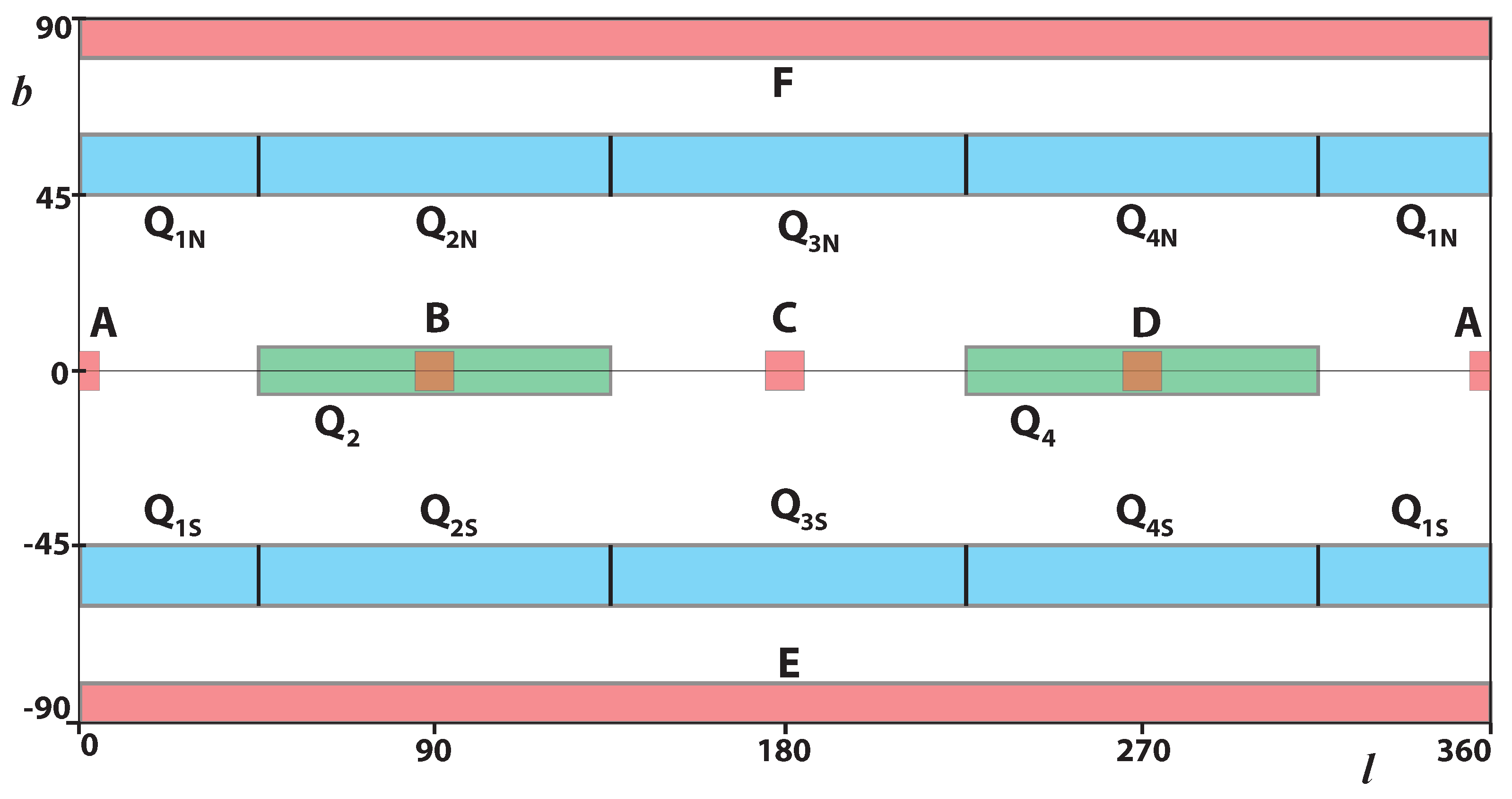
The data sectors of the sky used for analysis are defined in Figure 2 and Table 1. The narrow sectors A–F are defined by basic directions (from the Sun, see Figure 1): towards the centre of the galaxy (A), along the direction of galaxy rotation (B), and their opposites (C,D). The perpendiculars to the galactic disk define sectors E and F. The analysis is extended by other sectors: Q_α—in the galactic disk and ${\mathrm{Q}}_{\alpha \beta }$—outside the disk. We only accept sources with a positive parallax and limited distance $r<6$ kpc that satisfy the following condition:

$${\displaystyle \frac{\Delta v}{v}}\le \eta ;v=\left|{\mathbf{v}}_{gal}\right|=\left|{\mathbf{v}}_{ICRS}\right|,$$

(17)

whereby we set cuts for different sectors:

$$\begin{array}{cccc}\hfill \hfill & \hfill \mathrm{A}\hfill & \hfill \mathrm{B}-\mathrm{D}\hfill & \hfill \mathrm{E},\mathrm{F},\mathrm{Q}\hfill \\ \hfill \eta \hfill & \hfill 0.05\hfill & \hfill 0.2\hfill & \hfill 0.3\hfill \end{array}$$

In sectors from which we will determine our resulting velocities in Table 2, we use a more strict cut. Sector A contains regions of very high and inhomogeneous density and only a very safe cut $\eta$ gives consistent results compatible with the other sectors. We verified that the narrowing of these cuts does not systematically affect the curves, from which the resulting parameters are obtained. The error $\Delta v$ is estimated as

$${\left(\Delta v\right)}^2={\left({\displaystyle \frac{\partial v}{\partial p}}\Delta p\right)}^2+{\left({\displaystyle \frac{\partial v}{\partial {\mu }_{\alpha }^{\ast }}}\Delta {\mu }_{\alpha }^{\ast }\right)}^2+{\left({\displaystyle \frac{\partial v}{\partial {\mu }_{\delta }}}\Delta {\mu }_{\delta }\right)}^2.$$

(18)

Using Equation (12) expressed in ICRS and relation (13), we obtain the following ratio:

$${\displaystyle \frac{\Delta v}{v}}\approx \sqrt{{\left({\displaystyle \frac{\Delta p}{p}}\right)}^2+{\displaystyle \frac{{\left({\mu }_{\alpha }^{\ast }\Delta {\mu }_{\alpha }^{\ast }\right)}^2+{\left({\mu }_{\delta }\Delta {\mu }_{\delta }\right)}^2}{{\mu }^4}}};\mu =\sqrt{{\mu }_{\alpha }^{\ast 2}+{\mu }_{\delta }^2},$$

(19)

which is calculated from the Gaia data. The resulting numbers of accepted sources in the respective sectors are shown in the same table. Most of our calculations focus on mean values, which means that the resulting errors are much smaller than the errors of individual entries.

Figure 2. MW sectors used for analysis. Sectors B and D are subsets of sectors ${\mathrm{Q}}_2$ and ${\mathrm{Q}}_4$. Units: $b,l$ [deg].

Table 1. Number of stars in the analysed MW sectors: ${\mathrm{N}}_{tot}$—all stars, ${\mathrm{n}}_{cut}$—selected stars satisfying cut (17), and $⟨\mathrm{r}⟩$—mean distance of selected stars.

	A	B	C	D	E	F	${\mathrm{Q}}_2$	${\mathrm{Q}}_4$
$b[deg]$	$⟨-5,5⟩$				$⟨-90,-80⟩$	$⟨80,90⟩$	$⟨-5,5⟩$
$l[deg]$	$⟨-5,5⟩$	$⟨85,95⟩$	$⟨175,185⟩$	$⟨265,275⟩$	$⟨0,360⟩$		$⟨45.135⟩$	$⟨225,315⟩$
$⟨\mathrm{r}⟩\left[\mathrm{kpc}\right]$	1.02	1.89	1.63	1.84	0.90	0.93	1.93	2.08
${\mathrm{n}}_{cut}$	253,546	1,612,100	609,593	1,233,495	314,515	283,906	18,968,282	24,584,392
${\mathrm{N}}_{tot}$	22,704,200	6,646,423	2,498,909	5,422,928	573,436	540,330	70,260,517	85,849,109
H	${\mathrm{Q}}_{1S}$	${\mathrm{Q}}_{2S}$	${\mathrm{Q}}_{3S}$	${\mathrm{Q}}_{4S}$	${\mathrm{Q}}_{1N}$	${\mathrm{Q}}_{2N}$	${\mathrm{Q}}_{3N}$	${\mathrm{Q}}_{4N}$
$b[deg]$	$⟨-60,-45⟩$				$⟨45,60⟩$
$l[deg]$	$⟨-45,45⟩$	$⟨45,135⟩$	$⟨135.225⟩$	$⟨225,315⟩$	$⟨-45,45⟩$	$⟨45,135⟩$	$⟨135.225⟩$	$⟨225,315⟩$
$⟨\mathrm{r}⟩\left[\mathrm{kpc}\right]$	0.89	0.75	0.72	0.87	0.89	0.87	0.74	0.79
${\mathrm{n}}_{cut}$	1,646,264	1,161,311	995,955	1,475,289	1,378,017	1,337,495	977,358	1,052,616
${\mathrm{N}}_{tot}$	3,331,201	2,164,099	1,716,957	2,640,374	2,973,013	2,259,886	1,688,028	2,153,065

3. Methods and Results

In Figure 3, we show the distribution of star distances in the data sectors A–F defined above. The distance of most of them is $r\lesssim$ 3–6 kpc. Dependencies of mean velocities $⟨v_l⟩,⟨v_b⟩,⟨v_{gal}⟩$ and related standard deviations on distance r are shown in the figures that follow. What information can be extracted from them?

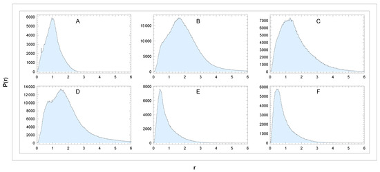
Figure 3. Distribution of distances in the sectors (A–F). Unit: r[kpc]. Binning: 0.024 kpc.

3.1. Velocity of the Sun

According to (8) and (15), the Sun’s velocity can be decomposed as

$${\mathbf{V}}_{\odot }={\mathbf{V}}_G\left({\mathbf{R}}_{\odot }\right)+\Delta {\mathbf{V}}_{\odot };{\mathbf{V}}_G\left({\mathbf{R}}_{\odot }\right)=-V_0\left(R_{\odot }\right){\mathbf{N}}_{\mathrm{\Phi }},$$

(20)

where ${\mathbf{V}}_G\left({\mathbf{R}}_{\odot }\right)$ is the LSR velocity and $\Delta {\mathbf{V}}_{\odot }$ is the Sun’s velocity in the LSR. How can these velocities be determined? In the galactic reference frame, the star velocity $\mathbf{v}\left(\mathbf{r}\right)$ is given as

$$\mathbf{v}\left(\mathbf{r}\right)=\mathbf{V}\left({\mathbf{R}}_{\odot }+\mathbf{r}\right)-{\mathbf{V}}_{\odot }={\mathbf{V}}_G\left({\mathbf{R}}_{\odot }+\mathbf{r}\right)+\Delta \mathbf{V}\left({\mathbf{R}}_{\odot }+\mathbf{r}\right)-{\mathbf{V}}_G\left({\mathbf{R}}_{\odot }\right)-\Delta {\mathbf{V}}_{\odot },$$

(21)

which implies

$$⟨⟨\mathbf{v}\left(\mathbf{r}\right)⟩⟩=⟨⟨\mathbf{V}\left({\mathbf{R}}_{\odot }+\mathbf{r}\right)⟩⟩-{\mathbf{V}}_G\left({\mathbf{R}}_{\odot }\right)-\Delta {\mathbf{V}}_{\odot }.$$

(22)

The region of averaging $⟨⟨...⟩⟩$$\left(\mathrm{over}\mathbf{r}\right)$ should be reasonably wide to suppress the influence of local fluctuations on the obtained average, and then the first two terms cancel, and for the local Sun’s velocity, we obtain

$$\Delta {\mathbf{V}}_{\odot }=-⟨⟨\mathbf{v}\left(\mathbf{r}\right)⟩⟩.$$

(23)

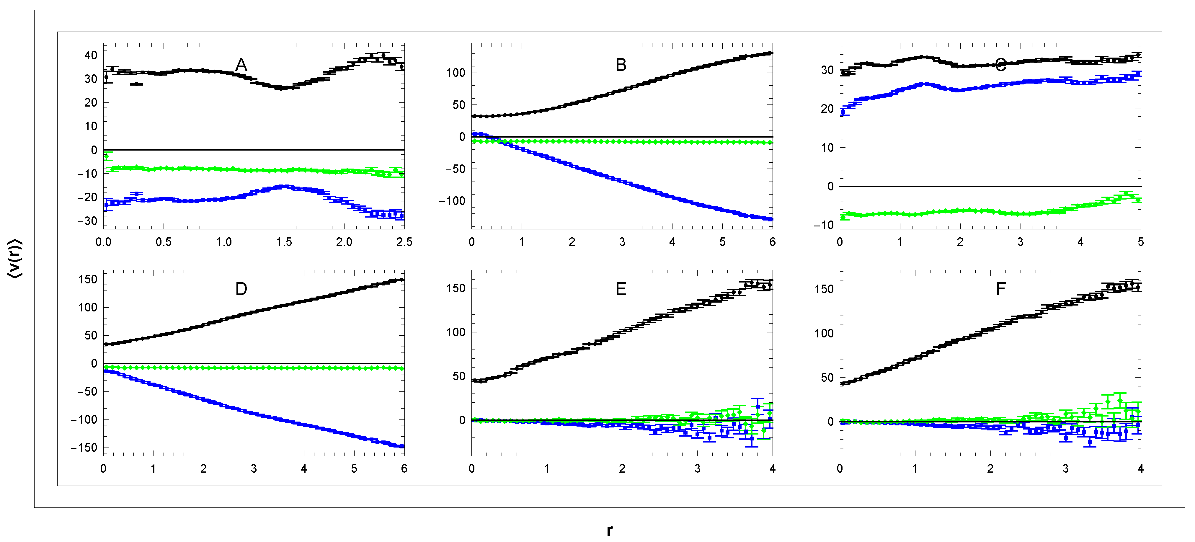
For its calculation, we use the projections of galactic velocities (12) in sectors A–D shown in Figure 4 together with the relations

$$v_l\left(\mathbf{r}\right)=\mathbf{v}\left(\mathbf{r}\right).{\mathbf{n}}_l,v_b\left(\mathbf{r}\right)=\mathbf{v}\left(\mathbf{r}\right).{\mathbf{n}}_b,$$

(24)

where the vectors of local orthonormal basis ${\mathbf{n}}_{\alpha }$ are defined in (7). In the sectors considered, we obtain

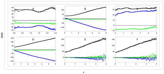
Figure 4. Dependence of mean velocity ($v_l$—blue, $v_b$—green, and $v_{gal}$—black) on distance r in the galactic reference frame in sectors (A–F). Units: r[kpc], v[km/s].

(1)

$\Delta V_{z\odot }$ in the sectors A–D

Since in these sectors we have ${\mathbf{n}}_b=\left(0,0,1\right),$ so we can identify $v_z=v_b$. The mean values $⟨v_b⟩$ depending on distance r are for individual sectors shown in Figure 4. The velocity $\Delta V_{z\odot }$ is the average:

$$\Delta V_{z\odot }\left(r_{max}\right)=-{⟨⟨v_z⟩⟩}_{\Omega },$$

(25)

where $\Omega$ means the region of averaging, which are the stars in the sectors A–D and radius $r<$$r_{max}$. The resulting curve is shown in Figure 5.

Figure 5. Velocities $\Delta V_{y\odot }$ (blue) and $\Delta V_{z\odot }$ (green) as the functions of ${\mathrm{r}}_{max}$ (left) with corresponding statistical errors (right). Units: ${\mathrm{r}}_{max}$[kpc], $\Delta V_{\alpha \odot }$[km/s].

(2)

$\Delta V_{y\odot }$ in the sectors A and C

In these sectors we have ${\mathbf{n}}_l=\left(0,\pm 1,0\right)$, so we identify $v_y=+v_l$ in the A and $v_y=-v_l$ in the C sector. The corresponding curves $⟨v_l⟩$ are in panels A,C (Figure 4) and curve

$$\Delta V_{y\odot }\left(r_{max}\right)=-{\displaystyle \frac{1}{2}}\left({⟨⟨v_y⟩⟩}_A+{⟨⟨v_y⟩⟩}_C\right)$$

(26)

is in Figure 5. The region of averaging are sectors A and C up to the distance $r_{max}.$

(3)

$\Delta V_{x\odot }$ and $V_0\left(R_0\right)$ in the sectors B and D

Here we have ${\mathbf{n}}_l=\left(\mp 1,0,0\right)$, so we can identify $v_x=-v_l$ in sector B and $v_x=+v_l$ in the D sector. In panels B,D in Figure 4, we show corresponding $⟨v_l⟩$ curves. For small r, we have $\Delta V_{x\odot }=-⟨v_x⟩$, which implies for B,D sectors,

$$\Delta V_{x\odot }=\pm ⟨v_l⟩.$$

(27)

but what is the reason for the steep slope of $⟨v_l⟩$ as r increases? In the considered sectors, the mean value $⟨v_l⟩$ includes a significant contribution from the collective rotation velocity ${\mathbf{V}}_G\left({\mathbf{R}}_{\odot }+\mathbf{r}\right)$ proportional to r, as explained below (Figure 9 and Equation (43)). Thus, in the B,D sectors, we have

$$⟨v_l^B⟩=\Delta V_{x\odot }-{\displaystyle \frac{r}{R}}{V}_0\left(R\right),⟨v_l^D⟩=-\Delta V_{x\odot }-{\displaystyle \frac{r}{R}}{V}_0\left(R\right);R=\sqrt{r^2+R_{\odot }^2}$$

(28)

and correspondingly,

$$⟨v_x^B⟩=-\Delta V_{x\odot }+{\displaystyle \frac{r}{R}}{V}_0\left(R\right),⟨v_x^D⟩=-\Delta V_{x\odot }-{\displaystyle \frac{r}{R}}{V}_0\left(R\right).$$

(29)

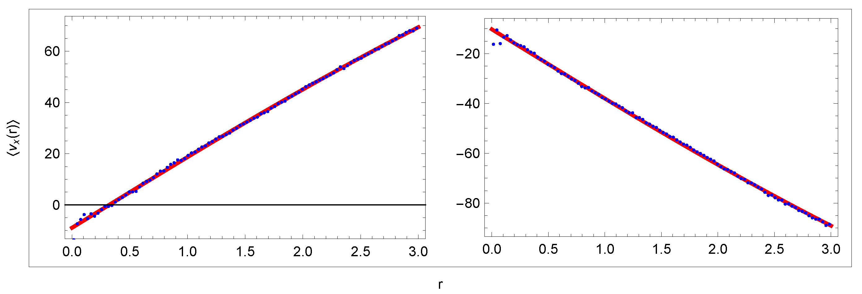
The two curves $⟨v_l⟩$ are shown in Figure 6 together with the curve produced by fitting the free parameters $\Delta V_{x\odot }$ and $V_0$ in the range $0<r<3$ kpc. Assuming that rotation velocity is constant in these sectors, $V_0\left(R\right)\approx V_0\left(R_{\odot }\right)$, we obtain very good agreement of the fit to the data. In the next, we abbreviate $V_0\left(R_{\odot }\right)$ by $V_0$. The obtained velocities are

$$\Delta V_{x\odot }^B=8.92,V_0^B=227.31;\Delta V_{x\odot }^D=10.23,V_0^D=228.86.$$

(30)

Admittedly, there is a weak dependency [6,8]:

$$V_0\left(R\right)=V_0-\kappa \left(R-R_{\odot }\right),$$

(31)

however, the range $0<r<3$ kpc means that $8.178<R<8.711$, which is too small a range for a reliable fit involving $\kappa$.

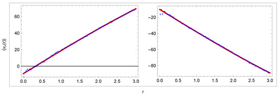
Figure 6. Curves (29): data (blue) and fit (red). Units: r[kpc], $v_x$[km/s].

In the left panel of Figure 5, we observe nearly constant curves while the right panel shows the dependence of corresponding statistical errors. The range of distances (0–3 kpc) involves the dominant part of analysed stars in sectors A–D. To estimate the Sun’s local velocity $\Delta V_{y\odot },\Delta V_{z\odot }$, we take the values in the middle of the range $\left(1.5\mathrm{kpc}\right)$. The velocities $\Delta V_{x\odot }$ and $V_0$ are obtained as averages of the values in (30).

However, for consistent comparison with other analyses, the velocities $\Delta V_{y\odot }$ and $V_0$ can require further correction based on the calculation of asymmetric drift (see [38], Section 11):

$$V_a=V_c-V_0,$$

(32)

where $V_c$ is the MW circular velocity at $R_{\odot }$ and $V_0$ is the mean orbital velocity of the stars in the neighbourhood of the Sun. The Sun orbital velocity $V_{\odot \mathrm{\Phi }}$ in the Galactocentric frame can be decomposed alternatively as

$$V_{\odot \mathrm{\Phi }}=V_0+\Delta V_{y\odot }=V_c+\Delta V_{y\odot }^{corr},$$

(33)

so

$$\Delta V_{y\odot }^{corr}=\Delta V_{y\odot }-V_a,V_c=V_0+V_a.$$

(34)

The study [39] estimates the asymmetric drift $V_a$ around the Sun’s position to be about 6 km/s. A very similar value can be extracted from Figure 3 in the paper [31], where the parameter $⟨v_R^2⟩$ is replaced by our parameter ${\sigma }_{R0}^2=1089$ km²${\mathrm{s}}^{-2}$, which is calculated in Table 3 in Section 3.3. In the standard notation, we can identify

$$U_{\odot }=\Delta V_{x\odot },V_{\odot }=\Delta V_{y\odot }-V_a,W_{\odot }=\Delta V_{z\odot },V_c=V_0+V_a,$$

(35)

where $\Delta V_{x\odot }$ and $V_0$ are the averages of the corresponding values in (30). We have

$$\Delta {\mathbf{V}}_{\odot }=\left(\Delta V_{x\odot },\Delta V_{y\odot },\Delta V_{z\odot }\right)=\left(9.58,22.25,7.33\right).$$

(36)

The associated velocities $U_{\odot },V_{\odot },W_{\odot },V_c$, and $V_0$ are shown in Table 2. Their systematic uncertainties are estimated as follows. For velocities $\Delta V_{y\odot },\Delta V_{z\odot }$, they are determined by the range of variability (defined as $\approx \left(max-min\right)$) of the curves in the left panel in interval $0.5<r_{max}<3$ kpc. For velocities $\Delta V_{x\odot }$ and $V_0$, systematic uncertainty is estimated similarly from a set of fits in different intervals of distances $\left(0<r<2,3,4,5\mathrm{kpc}\right)$. The relatively small systematic uncertainty in $V_0$ reflects the relatively small local variations.

Table 2. Local velocity of the Sun (with statistical errors), mean rotation velocity $V_0$, circular velocity $V_c$, and their systematic errors ${\Delta }_{syst}$ along with the results of other analyses. Units: [km/s].

${\mathit{U}}_{\odot }$	${\mathit{V}}_{\odot }$	${\mathit{W}}_{\odot }$	${\mathit{V}}_0$	${\mathit{V}}_{\mathit{c}}$	${\mathit{\Delta }}_{\mathbf{syst}}$	${\mathit{V}}_{\mathit{c}}+{\mathit{V}}_{\odot }$	Ref.
$9.58\pm 0.05$	$16.25\pm 0.04$	$7.33\pm 0.02$	228	234	$\left(0.7,0.9,0.1,4.0,4.0\right)$	$251.0\pm 5$	this work
$11.1_{-0.75}^{+0.69}$	$12.24\pm 0.47$	$7.{25}_{-0.36}^{+0.37}$			$\left(1,2,0.5,-\right)$		[31]
$9.12\pm 0.10$	$20.80\pm 0.10$	$7.66\pm 0.08$	$230\pm 12$			$250.8$	[40]
$9.58\pm 2.39$	$10.52\pm 1.96$	$7.01\pm 1.67$					[41]
$10.00\pm 0.36$	$5.25\pm 0.62$	$7.17\pm 0.38$					[42]
	$14.6\pm 5$			$240\pm 8$		$255.2\pm 5.1$	[8]
	$26\pm 3$			$218\pm 6$		${242}_{-3}^{+10}$	[43]
$7.7\pm 0.9$	$12.4\pm 0.7$			$236\pm 3$		$248.4$	[24]
	$12.1\pm 7.6$			$240\pm 6$		$252.1$	[11]
$\approx 11.1$		$\approx 7.8$		$229\pm 0.2$	$\left(-,-,-,\approx 2\%-5\%\right)$	$\approx 245.8$	[6]
	$24\pm 1$				$\pm 2\left(V_c\right)\pm 5\left(\mathrm{large}\mathrm{scale}\right)$		[44]
				$238\pm 9$		$250\pm 9$	[45]
				$233.6\pm 2.8$			[7]
			$\approx 230$				[17]
				$224\pm 13$			[46]
				$217\pm 6$			[13]
						$247.4\pm 1.4$	[29]
						$253\pm 6$	[47]

Table 2. Local velocity of the Sun (with statistical errors), mean rotation velocity $V_0$, circular velocity $V_c$, and their systematic errors ${\Delta }_{syst}$ along with the results of other analyses. Units: [km/s].

${\mathit{U}}_{\odot }$	${\mathit{V}}_{\odot }$	${\mathit{W}}_{\odot }$	${\mathit{V}}_0$	${\mathit{V}}_{\mathit{c}}$	${\mathit{\Delta }}_{\mathbf{syst}}$	${\mathit{V}}_{\mathit{c}}+{\mathit{V}}_{\odot }$	Ref.
$9.58\pm 0.05$	$16.25\pm 0.04$	$7.33\pm 0.02$	228	234	$\left(0.7,0.9,0.1,4.0,4.0\right)$	$251.0\pm 5$	this work
$11.1_{-0.75}^{+0.69}$	$12.24\pm 0.47$	$7.{25}_{-0.36}^{+0.37}$			$\left(1,2,0.5,-\right)$		[31]
$9.12\pm 0.10$	$20.80\pm 0.10$	$7.66\pm 0.08$	$230\pm 12$			$250.8$	[40]
$9.58\pm 2.39$	$10.52\pm 1.96$	$7.01\pm 1.67$					[41]
$10.00\pm 0.36$	$5.25\pm 0.62$	$7.17\pm 0.38$					[42]
	$14.6\pm 5$			$240\pm 8$		$255.2\pm 5.1$	[8]
	$26\pm 3$			$218\pm 6$		${242}_{-3}^{+10}$	[43]
$7.7\pm 0.9$	$12.4\pm 0.7$			$236\pm 3$		$248.4$	[24]
	$12.1\pm 7.6$			$240\pm 6$		$252.1$	[11]
$\approx 11.1$		$\approx 7.8$		$229\pm 0.2$	$\left(-,-,-,\approx 2\%-5\%\right)$	$\approx 245.8$	[6]
	$24\pm 1$				$\pm 2\left(V_c\right)\pm 5\left(\mathrm{large}\mathrm{scale}\right)$		[44]
				$238\pm 9$		$250\pm 9$	[45]
				$233.6\pm 2.8$			[7]
			$\approx 230$				[17]
				$224\pm 13$			[46]
				$217\pm 6$			[13]
						$247.4\pm 1.4$	[29]
						$253\pm 6$	[47]

3.2. Rotation Curves

From now, we will substitute galactic velocity $\mathbf{v}\left(\mathbf{r}\right)$ in Equation (21) by $\mathbf{v}\left(\mathbf{r}\right)$$\to \mathbf{v}\left(\mathbf{r}\right)+\Delta {\mathbf{V}}_{\odot }$, which is the velocity related to the LSR:

$$\begin{array}{cc}\hfill \mathbf{v}\left(\mathbf{r}\right)& ={\mathbf{V}}_G\left(\mathbf{R}\right)+\Delta \mathbf{v}\left(\mathbf{R}\right)-{\mathbf{V}}_G\left({\mathbf{R}}_{\odot }\right),\hfill \end{array}$$

(37)

$$\begin{array}{cc}\hfill ⟨\mathbf{v}\left(\mathbf{r}\right)⟩& ={\mathbf{V}}_G\left({\mathbf{R}}_{\odot }+\mathbf{r}\right)-{\mathbf{V}}_G\left({\mathbf{R}}_{\odot }\right).\hfill \end{array}$$

(38)

In this frame, the input data in Equation (12) are modified with the use of our $\Delta {\mathbf{V}}_{\odot }$ as

$$\begin{array}{cc}\hfill v_l& \to v_l+\Delta {\mathbf{V}}_{\odot }.{\mathbf{n}}_l,v_b\to v_b+\Delta {\mathbf{V}}_{\odot }.{\mathbf{n}}_b,\hfill \end{array}$$

(39)

$$\begin{array}{cc}\hfill v_{gal}& \to \sqrt{{\left(v_l+\Delta {\mathbf{V}}_{\odot }.{\mathbf{n}}_l\right)}^2+{\left(v_b+\Delta {\mathbf{V}}_{\odot }.{\mathbf{n}}_b\right)}^2}.\hfill \end{array}$$

(40)

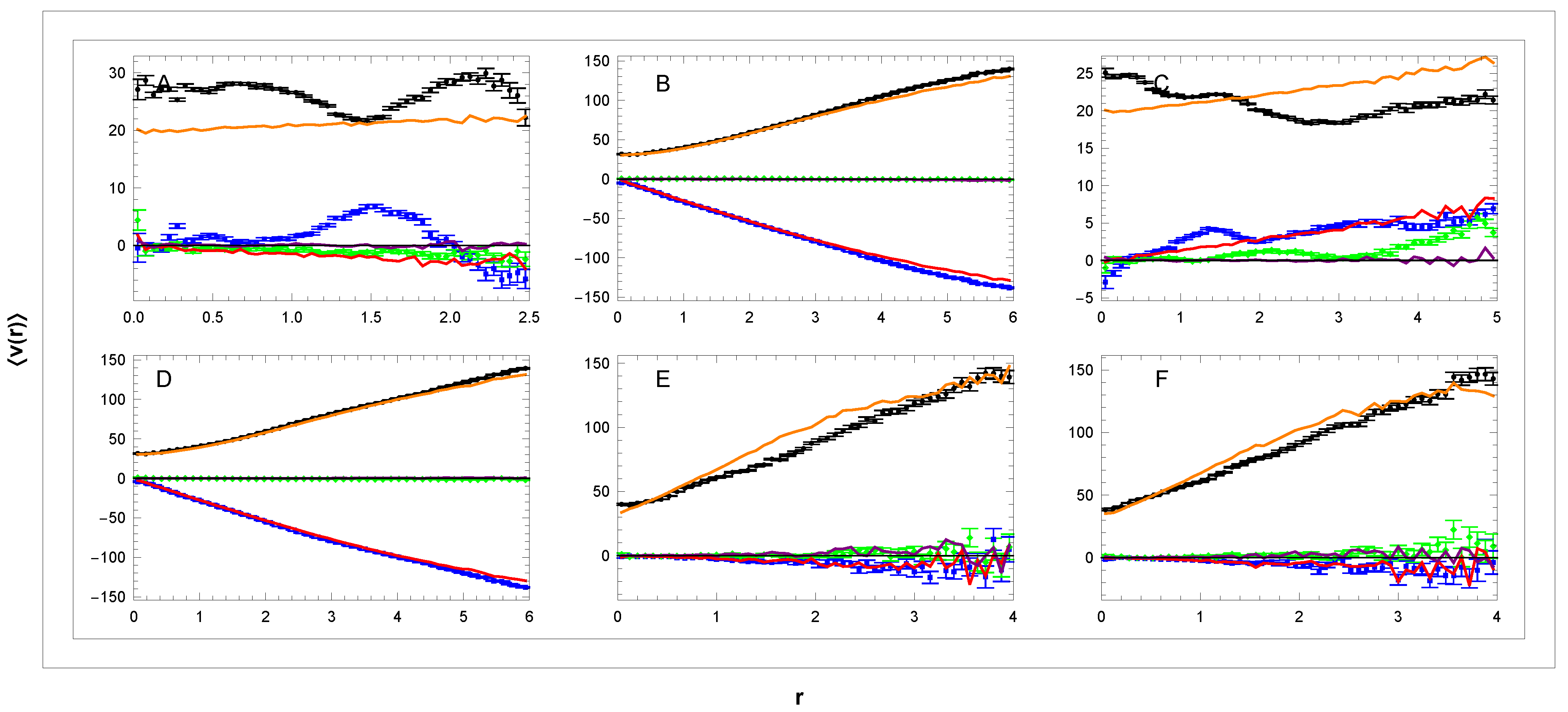
After this substitution, Figure 4 is replaced by the top panel in Figure 7. The new $v_l,v_b,v_{gal}$ refer to the LSR whose velocity is

$${\mathbf{V}}_{LSR}={\mathbf{V}}_G\left({\mathbf{R}}_{\odot }\right)=\left(0,V_0,0\right).$$

(41)

The combination of the new panels A and C, which represents the RC, is shown in Figure 8a.

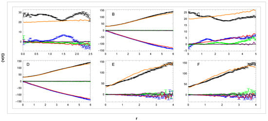
Figure 7. Dependence of mean velocity ($v_l$—blue, $v_b$—green, and $v_{gal}$—black) on distance r in the local rest frame at ${\mathbf{R}}_{\odot }$ in sectors (A–F). For the corresponding curves ($v_l$—red, $v_b$—purple, and $v_{gal}$—orange) of the simulation model, see Section 3.3 and Section 3.4. Units: r[kpc], v[km/s].

Figure 8. Velocity curves $V=V_0\left(R\right)-V_0\left(R_{\odot }\right)$ in sectors A+C (panel (a)) and $V=V_0\left(R\right)$ in sectors B and D (panels (b,c)). Units: R[kpc], v[km/s].

Another representation of the RC is obtained from panels B and D. For $\left|Z\right|\approx 0$ and $r>0,$ the term $\mathbf{w}={\mathbf{V}}_G\left({\mathbf{R}}_{\odot }+\mathbf{r}\right)-{\mathbf{V}}_G\left({\mathbf{R}}_{\odot }\right)$ in Equation (38) and its transverse projection $⟨w_l⟩$ are calculated as suggested in Figure 9 from two similar orthogonal triangles with angle $\alpha .$ We obtain

$$⟨w_l⟩={\displaystyle \frac{r}{R}}{V}_0\left(R\right);R=\sqrt{r^2+R_{\odot }^2}.$$

(42)

Since $w_l=-v_l$, we obtain

$$\begin{array}{cc}\hfill ⟨v_l⟩& =-{\displaystyle \frac{r}{R}}{V}_0\left(R\right),\hfill \end{array}$$

(43)

$$\begin{array}{cc}\hfill V_0\left(R\right)& =-{\displaystyle \frac{R}{r}}⟨v_l⟩.\hfill \end{array}$$

(44)

The corresponding RCs are shown in panels b,c of Figure 8. These curves are a different representation of the $⟨v_l⟩$ curves in panels B and D of Figure 7.

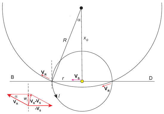
Figure 9. Rotation of MW as seen in sectors B and D. Here the symbols ${\mathbf{V}}_{\mathbf{R}}$ and ${\mathbf{V}}_{\mathbf{S}}$ stand for ${\mathbf{V}}_G\left(\mathbf{R}\right)$ and ${\mathbf{V}}_G\left({\mathbf{R}}_{\odot }\right)$.

Relation (43) holds only for sectors B and D, where $l\approx \pm \pi /2$ and $Z\approx 0$ (or $b\approx 0$). In the general case, the geometry is more complicated. With the use of (24) and (38), we have

$$⟨v_l⟩=\left({\mathbf{V}}_G\left({\mathbf{R}}_{\odot }+\mathbf{r}\right)-{\mathbf{V}}_G\left({\mathbf{R}}_{\odot }\right)\right).{\mathbf{n}}_l.$$

(45)

This relation can be modified as

$$⟨v_l⟩=-\left(V_G\left({\mathbf{R}}_{\odot }+\mathbf{r}\right){\mathbf{N}}_{\mathrm{\Phi }}\left({\mathbf{R}}_{\odot }+\mathbf{r}\right)-V_0{\mathbf{N}}_{\mathrm{\Phi }}\left({\mathbf{R}}_{\odot }\right)\right).{\mathbf{n}}_l.$$

(46)

With the use of relations (6), (3), and (1), vector ${\mathbf{N}}_{\mathrm{\Phi }}$ can be expressed in galactic coordinates $r,l,b$, and after a few further modifications, we obtain

$$⟨v_l⟩=\gamma V_G\left({\mathbf{R}}_{\odot }+\mathbf{r}\right)-V_{0}cosl$$

(47)

and if $\gamma \ne 0$, then

$$V_G\left({\mathbf{R}}_{\odot }+\mathbf{r}\right)={\displaystyle \frac{⟨v_l⟩+V_{0}cosl}{\gamma }};\gamma ={\displaystyle \frac{R_{\odot }cosl-rcosb}{\sqrt{R_{\odot }^2+r^2{cos}^{2}b-2R_{\odot }rcoslcosb}}}.$$

(48)

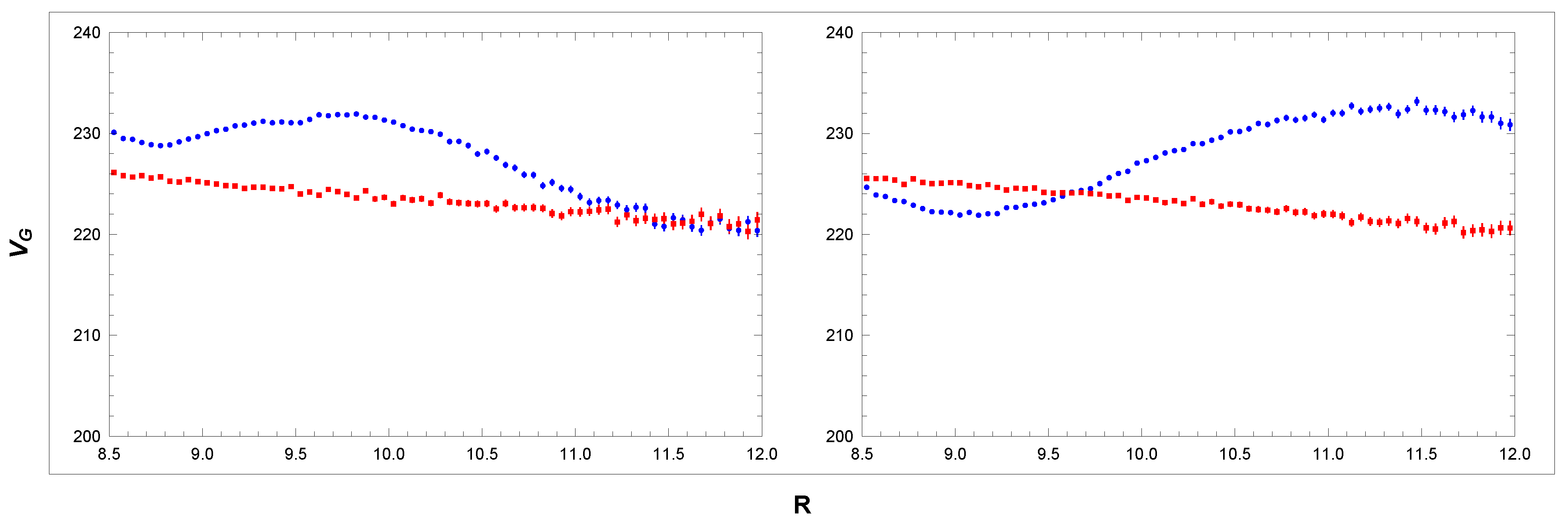
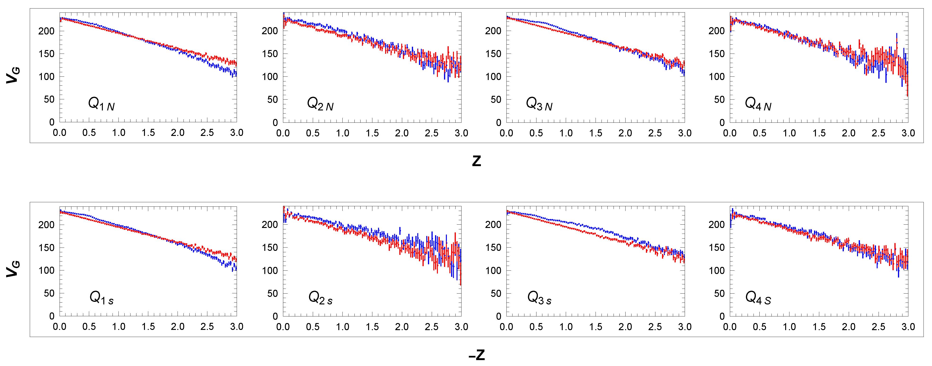
One can check that in sectors B and D, where $b\approx 0$, $l\approx \pm \pi /2$ and where we have assumed $V_G\approx V_0\left(R\right)$, relation (47) reduces to (43). Relation (48) allows us to analyse $V_G\left(\mathbf{R}\right)$ not only in narrow sectors B and D but also in the wider regions, which can provide higher statistics with smaller errors. This relation is not suitable for the reconstruction of $V_G$ in the vicinity of singularity $\gamma \approx 0$ $\left(R_{\odot }cosl\approx rcosb\right)$. In Figure 10 (blue points), we show RCs obtained with the use of Equation (48) in the sectors ${\mathrm{Q}}_2$ and ${\mathrm{Q}}_4$. In the analysed area, we observe irregular fluctuations in the rotation velocity: $\Delta V_G/V_G\approx 5\%$. The relation allows us to calculate rotation velocity not only in the galactic plane but also outside the plane. In Figure 11, we show the velocity curves $V_G\left(\left|Z\right|\right)$ calculated in sectors ${\mathrm{Q}}_{1S}-$ ${\mathrm{Q}}_{4S}$ and ${\mathrm{Q}}_{1N}-$ ${\mathrm{Q}}_{4N}$.

Figure 10. RCs in sectors ${\mathrm{Q}}_2$ (left) and ${\mathrm{Q}}_4$ (right): data (blue) and simulation (red). For simulated curves, see Section 3.3 and Section 3.4. Units: R[kpc], $V_G$[km/s].

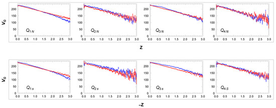
Figure 11. Velocity curves $V_G\left(\left|Z\right|\right)$ in sectors ${\mathrm{Q}}_{1S}-$ ${\mathrm{Q}}_{4S}$ and ${\mathrm{Q}}_{1N}-$${\mathrm{Q}}_{4N}$: data (blue) and simulation (red). For simulated curves, see Section 3.3 and Section 3.4. Units: Z[kpc], $V_G$[km/s].

3.3. Six Parameters of the MW Collective Rotation

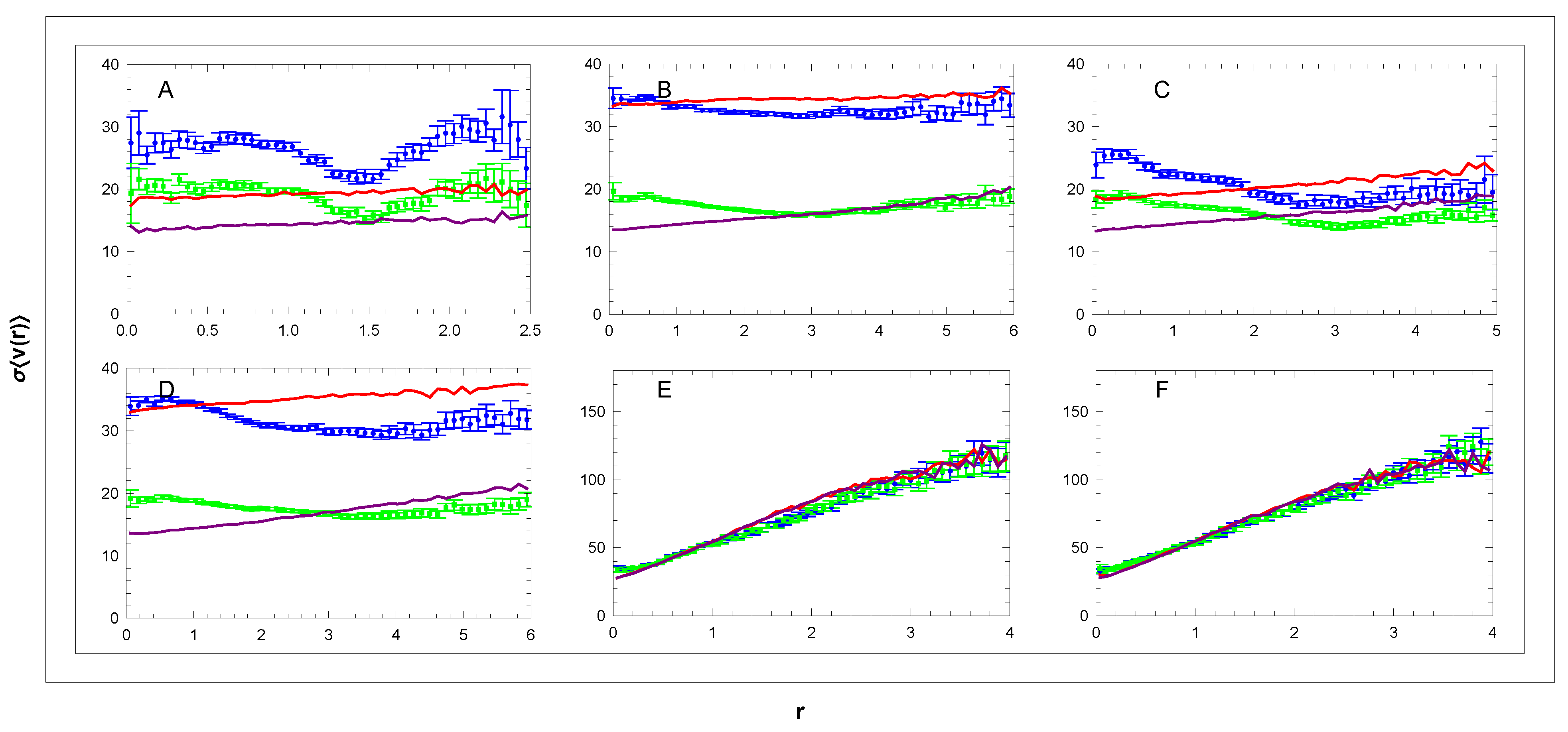
Panels E and F at the top of Figure 7 provide further important information. We observe $⟨v_l⟩\approx 0$ and $⟨v_b⟩\approx 0$, as expected in both narrow cones pointing perpendicularly from the galactic plane, where positive and negative $v_l,v_b$ are equally abundant. On the other hand, the value $⟨v_{gal}⟩$ increases with distance from the plane. This increase occurs in the galactic reference frame reflecting the slowing of collective rotation in the Galactocentric frame, which increases with $r\approx \left|Z\right|$. The same effect is seen even more clearly in Figure 11. Important information is obtained from Figure 12, where dependencies of standard deviations are shown. The increasing standard deviations in panels E and F suggest a less collective but more disorderly motion of high velocities away from the galactic plane.

Figure 12. Dependence of the standard deviations of the mean velocity ($v_l$—blue and $v_b$—green) on the distance r in sectors (A–F). For simulated curves ($v_l$—red and $v_b$—purple), see Section 3.4. Units: r[kpc], $\sigma$[km/s].

In the distribution (16), we assume in a first approximation that

$${\sigma }_{\alpha }={\sigma }_{\alpha 0}+{\sigma }_{\alpha 1}\left|Z\right|;\alpha =R,\mathrm{\Theta },\mathrm{\Phi },$$

(49)

where ${\sigma }_{\alpha 0}$ and ${\sigma }_{\alpha 1}$ are the free parameters. We proceed as follows in their setting:

(i) From the data panels A–D in Figure 12 where $Z\approx 0$, we estimate the first approximation:

$$\begin{array}{cc}\hfill {\sigma }_{\mathrm{\Theta }0}& \approx ⟨{\sigma }_b⟩\mathrm{in}\sec \mathrm{tors}\mathrm{A}–\mathrm{D},\hfill \end{array}$$

(50)

$$\begin{array}{cc}\hfill {\sigma }_{R0}& \approx ⟨{\sigma }_l⟩\mathrm{in}\sec \mathrm{tors}\mathrm{B},\mathrm{D}\mathrm{and}\mathrm{at}\mathrm{small}r/R_{\odot },\hfill \end{array}$$

(51)

$$\begin{array}{cc}\hfill {\sigma }_{\mathrm{\Phi }0}& \approx ⟨{\sigma }_l⟩\mathrm{in}\sec \mathrm{tors}\mathrm{A},\mathrm{C}.\hfill \end{array}$$

(52)

In directions other than A–D, the relations between $\sigma$s in the galactic and Galactocentric frames are more complex. The final tuning of these three parameters is performed in Section 3.4 using further curves.

(ii) The data panels E and F (where $r\approx \left|Z\right|$) show in the region of the peaks ($r\lesssim 2.5$ kpc, see Figure 3, panels E,F) a linear increase in the corresponding mixture of $\sigma$s with $\left|Z\right|$. To obtain the parameters ${\sigma }_{\alpha 1}$, we analysed the respective distributions in all the sectors listed in Table 1. We found that the optimal shape of the distribution $V_{\mathrm{\Phi }}$ in (16) is asymmetric, having different ${\sigma }_{\mathrm{\Phi }}^{\pm }$ for the two opposite orientations, where $+(-)$ means in (against) the rotation direction:

$${\sigma }_{\mathrm{\Phi }}^{+}={\sigma }_{\mathrm{\Phi }0},{\sigma }_{\mathrm{\Phi }}^{-}={\sigma }_{\mathrm{\Phi }0}+{\sigma }_{\mathrm{\Phi }1}^{-}\left|Z\right|.$$

(53)

So only ${\sigma }_{\mathrm{\Phi }}^{-}$ depends on $\left|Z\right|$ and ${\sigma }_{\mathrm{\Phi }}^{+}$ does not. This asymmetry also reflects the effective deceleration $⟨\Delta V_{\mathrm{\Phi }}⟩$ of the collective rotation for larger $\left|Z\right|$ as mentioned above. We have

$$\begin{array}{c}\hfill ⟨\Delta V_{\mathrm{\Phi }}⟩={\displaystyle \frac{1}{N}}\left({\int }_{-\infty }^0{V}_{\mathrm{\Phi }}exp\left(-{\displaystyle \frac{1}{2}}{\left({\displaystyle \frac{V_{\mathrm{\Phi }}}{{\sigma }_{\mathrm{\Phi }}^{-}}}\right)}^2\right)d{V}_{\mathrm{\Phi }}+{\int }_0^{\infty }{V}_{\mathrm{\Phi }}exp\left(-{\displaystyle \frac{1}{2}}{\left({\displaystyle \frac{V_{\mathrm{\Phi }}}{{\sigma }_{\mathrm{\Phi }}^{+}}}\right)}^2\right)d{V}_{\mathrm{\Phi }}\right);\\ \hfill N={\int }_{-\infty }^{0}exp\left(-{\displaystyle \frac{1}{2}}{\left({\displaystyle \frac{V_{\mathrm{\Phi }}}{{\sigma }_{\mathrm{\Phi }}^{-}}}\right)}^2\right)d{V}_{\mathrm{\Phi }}+{\int }_0^{\infty }exp\left(-{\displaystyle \frac{1}{2}}{\left({\displaystyle \frac{V_{\mathrm{\Phi }}}{{\sigma }_{\mathrm{\Phi }}^{+}}}\right)}^2\right)d{V}_{\mathrm{\Phi }}.\end{array}$$

(54)

After integration we obtain

$$⟨\Delta V_{\mathrm{\Phi }}⟩=\sqrt{{\displaystyle \frac{2}{\pi }}}\left({\sigma }_{\mathrm{\Phi }}^{+}-{\sigma }_{\mathrm{\Phi }}^{-}\right)=-\sqrt{{\displaystyle \frac{2}{\pi }}}{\sigma }_{\mathrm{\Phi }1}^{-}\left|Z\right|.$$

(55)

The important parameter ${\sigma }_{\mathrm{\Phi }1}^{-}$ is obtained by the fit from Figure 11, which suggests dependence:

$$\begin{array}{c}\hfill V_G\left(\left|Z\right|\right)=V_0+⟨\Delta V_{\mathrm{\Phi }}⟩\approx V_0-\varkappa \left|Z\right|;\varkappa =\sqrt{{\displaystyle \frac{2}{\pi }}}{\sigma }_{\mathrm{\Phi }1}^{-}\doteq 33.5\mathrm{km}{\mathrm{s}}^{-1}{\mathrm{kpc}}^{-1}.\end{array}$$

(56)

For the remaining two parameters, the analysis showed that ${\sigma }_{\mathrm{\Theta }1}$ $\approx {\sigma }_{R1}$ is a good approximation. We denote ${\sigma }_1$ $\equiv {\sigma }_{R1}={\sigma }_{\mathrm{\Theta }1}$: this last free parameter was set up from the tuning of the slope in simulation panels E and F in Figure 12. A list of the six resulting parameters controlling simulation (16) is given in Table 3. The relation (56) shows that the MW rotation at $Z_{\odot }\approx 0.0208$ kpc is $0.7$ km/s lower than at $Z=0$, which is significantly less than the total error in determining $V_0$. Therefore, we neglected $Z_{\odot }$ in our calculation. The Wolfram Mathematica code of the generator is available on the website https://www.fzu.cz/~piska/Catalogue/genkinJAN25.nb (accessed on 20 January 2025). Figure 13 shows the examples of the distribution of simulated velocities $V_{\mathrm{\Phi }},V_{\mathrm{\Theta }}$, and $V_R$. The simulated distributions $V_{\mathrm{\Theta }}$ and $V_R$ are symmetric for any $\left|Z\right|$, and distribution $V_{\mathrm{\Phi }}$ is asymmetric for $\left|Z\right|>0$.

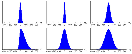
Figure 13. Distribution of simulated velocities $V_{\mathrm{\Phi }},V_{\mathrm{\Theta }}$, and $V_R$ at $Z=0$ (upper row) and $Z=1.5$ kpc (lower row). Units: V[km/s].

Table 3. Monte Carlo simulation model parameters and corresponding parameters from other analyses. Velocity $V_0$ is taken from Table 2.

${\mathit{\sigma }}_{\mathit{\Theta }0}$ [km s−1]	${\mathit{\sigma }}_{\mathit{\Phi }0}$ [km s−1]	${\mathit{\sigma }}_{\mathit{R}0}$ [km s−1]	${\mathit{\sigma }}_1$ [km s−1kpc−1]	${\mathit{\sigma }}_{\mathit{\Phi }1}^{-}$ [km s−1kpc−1]	${\mathit{V}}_0$ [km s−1]	Ref.
13	18	33	24	42	228	this work
$18.03\pm 0.03$	$24.35\pm 0.04$	$36.81\pm 0.07$	x	x	x	[48]
11	20	31	x	x	x	[49]

Table 3. Monte Carlo simulation model parameters and corresponding parameters from other analyses. Velocity $V_0$ is taken from Table 2.

${\mathit{\sigma }}_{\mathit{\Theta }0}$ [km s−1]	${\mathit{\sigma }}_{\mathit{\Phi }0}$ [km s−1]	${\mathit{\sigma }}_{\mathit{R}0}$ [km s−1]	${\mathit{\sigma }}_1$ [km s−1kpc−1]	${\mathit{\sigma }}_{\mathit{\Phi }1}^{-}$ [km s−1kpc−1]	${\mathit{V}}_0$ [km s−1]	Ref.
13	18	33	24	42	228	this work
$18.03\pm 0.03$	$24.35\pm 0.04$	$36.81\pm 0.07$	x	x	x	[48]
11	20	31	x	x	x	[49]

3.4. Comparison of Simulation Model with Data

The comparison is performed as follows:

(1) The position $\left(r,l,b\right)$ of the source in the galactic reference frame is with the use of Equation (3) transformed to the Galactocentric spherical frame $\left(R,\mathrm{\Phi },\mathrm{\Theta }\right)$. For this position, the velocity ${\mathbf{V}}^{gen}\left(\mathbf{R}\right)$ defined by (14) is generated according to distribution (16) with the parameters from Table 3.

(2) Using (41) and (7) we obtain the corresponding LSR transverse velocities:

$$v_{\alpha }^{gen}\left(\mathbf{r}\right)=\left({\mathbf{V}}^{gen}\left(\mathbf{R}\right)-{\mathbf{V}}_{LSR}\right).{\mathbf{n}}_{\alpha };\alpha =l,b.$$

(57)

So for any source defined by input $\left(r,l,b,v_l,v_b\right),$ we generate a vector $\left(r,l,b,v_l^{gen},v_b^{gen}\right)$ and then create the desired distributions from both.

(3) These distributions obtained from the input data and simulations will now be compared. The comparison in Figure 7 shows overall very good agreement between data and simulation for panels B,D,E,F. In panels A and C, the simulation model does not reproduce local kinematic substructures generating deviations $\Delta v\lesssim 10$ km/s. The presence of these substructures shows the precision with which we work. At the same time, the fluctuations are not noticeable in the other panels because their velocity scale is coarser.

The simulation in panel A(C) indicates that the velocity ${⟨v_l\left(r\right)⟩}_S$ decreases (increases) with r, despite the constant parameter $V_0$. This small effect is because we are working inside the angle $b=\pm 5$ deg, which means a slight linear increase in average $\left|Z\right|$ and correspondingly some deceleration with r. So, a corresponding correction would therefore be necessary to evaluate the RC in this sector more accurately. We checked that for smaller angles $\left|b\right|$, this effect disappears.

Figure 12 shows the corresponding velocity dispersion dependencies. In the upper panels A–D, we again observe fluctuations that are not present in the simulation. In panels E,F with a coarser scale, the fluctuations are not noticeable, and agreement with the simulation is very good. Averaged data in panels B-D do not contradict the simulation. The difference between data and simulation in panel A is more obvious and will be analysed below.

Relatively small velocity fluctuations ($\Delta V_G\lesssim 10$ km/s, $\Delta V_G/V_G\lesssim 0.05$) also appear in the RC in Figure 10. The slightly decreasing simulated RC is due to the shape of the sectors ${\mathrm{Q}}_2$ and ${\mathrm{Q}}_4$, where a larger R correlates with a larger average $\left|Z\right|$, implying a smaller $V_G$. Figure 11 shows that the simulation of decreasing $V_G\left(\left|Z\right|\right)$ controlled by the fitted parameter ${\sigma }_{\mathrm{\Phi }1}^{-}$ in Equation (56) agrees well with the data.

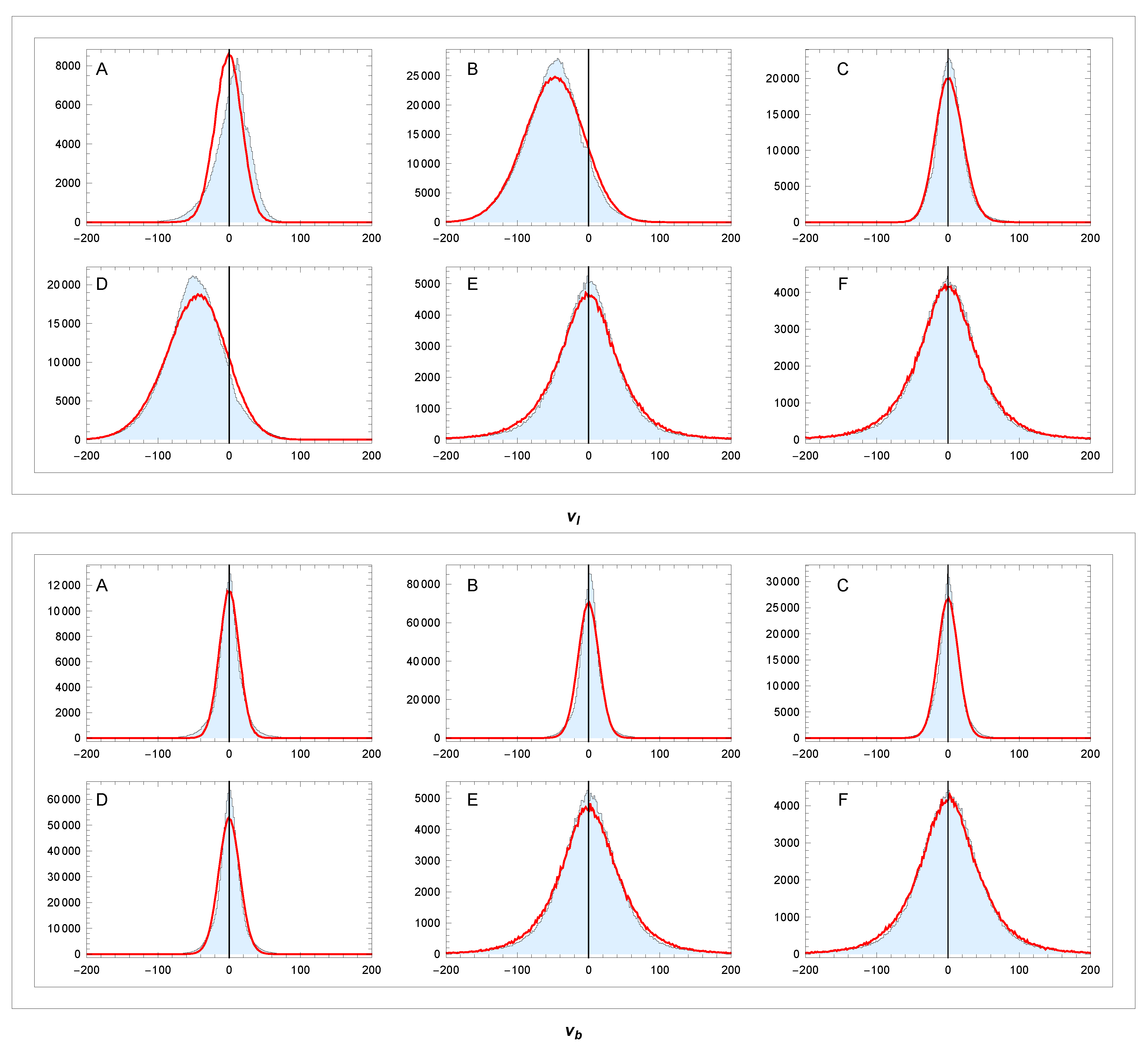
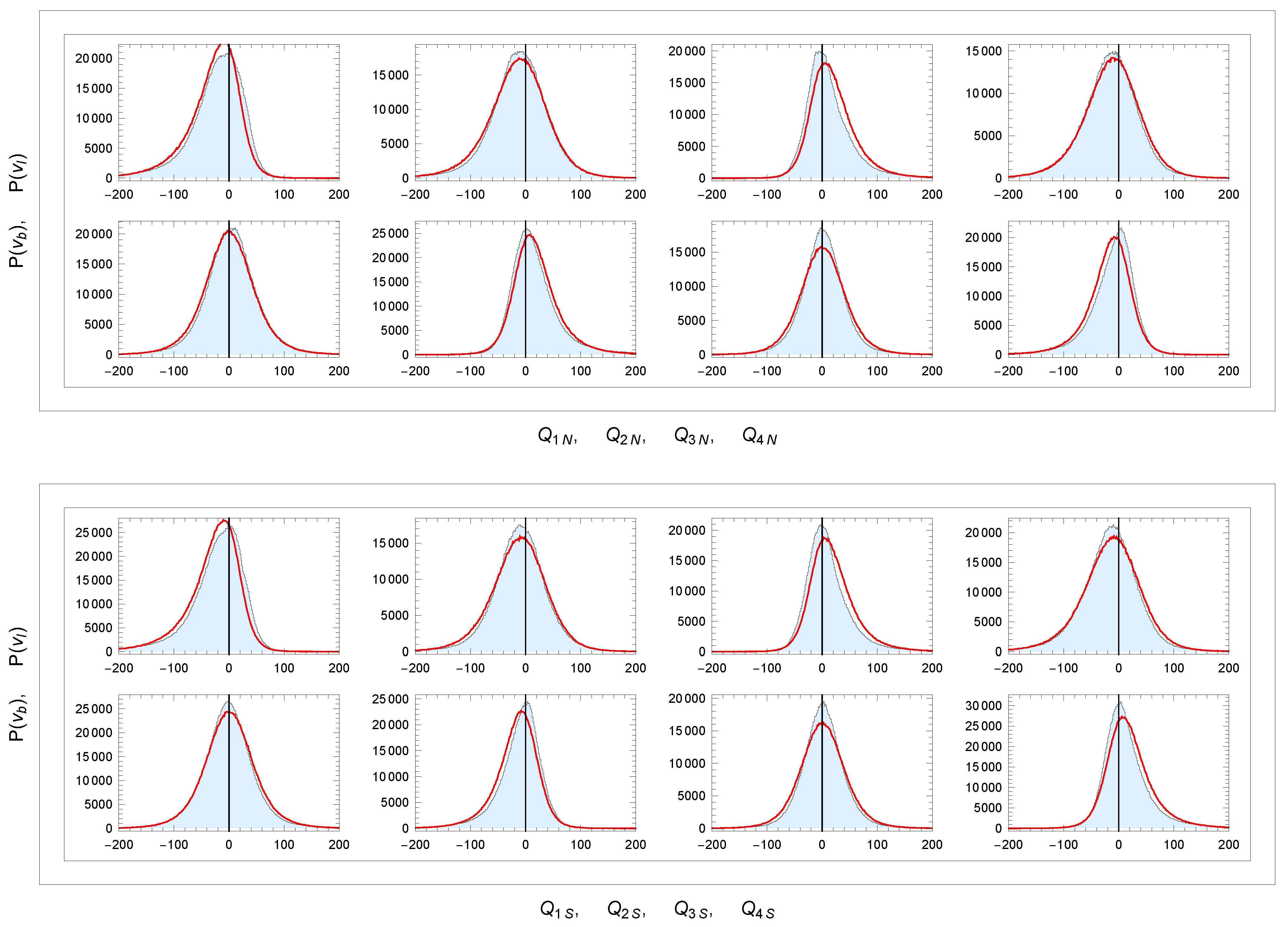
The good agreement of the simulations with the data is confirmed by other results. Figure 14 shows distributions of $v_l$ and $v_b$ in sectors A–F along with the corresponding distributions obtained from simulations. With the help of this data, the final tuning of the parameters ${\sigma }_{\mathrm{\Theta }0}$ and ${\sigma }_{\mathrm{\Phi }0}$ was achieved. An apparent disagreement with the simulation occurs in sector A (where $R<R_{\odot }$). It may be a manifestation of the asymmetric drift effect. In the opposite sector C (where $R>R_{\odot }$), the asymmetry is not manifested. The distributions of $v_l$ in both sectors A and C are copies (up to a constant shift) of the distribution of orbital velocities in the Galactocentric frame. Note the shift in sectors B and D resulting from the decrease in $⟨v_l⟩$ in panels B and D in Figure 7. As expected, there is a clear symmetry between the two panels.

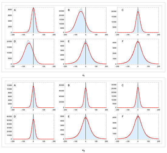
Figure 14. Distributions of $v_l$ and $v_b$ in sectors (A–F): data (light blue) and simulation model (red). Unit: v[km/s]. Binning: 1.6 km/s.

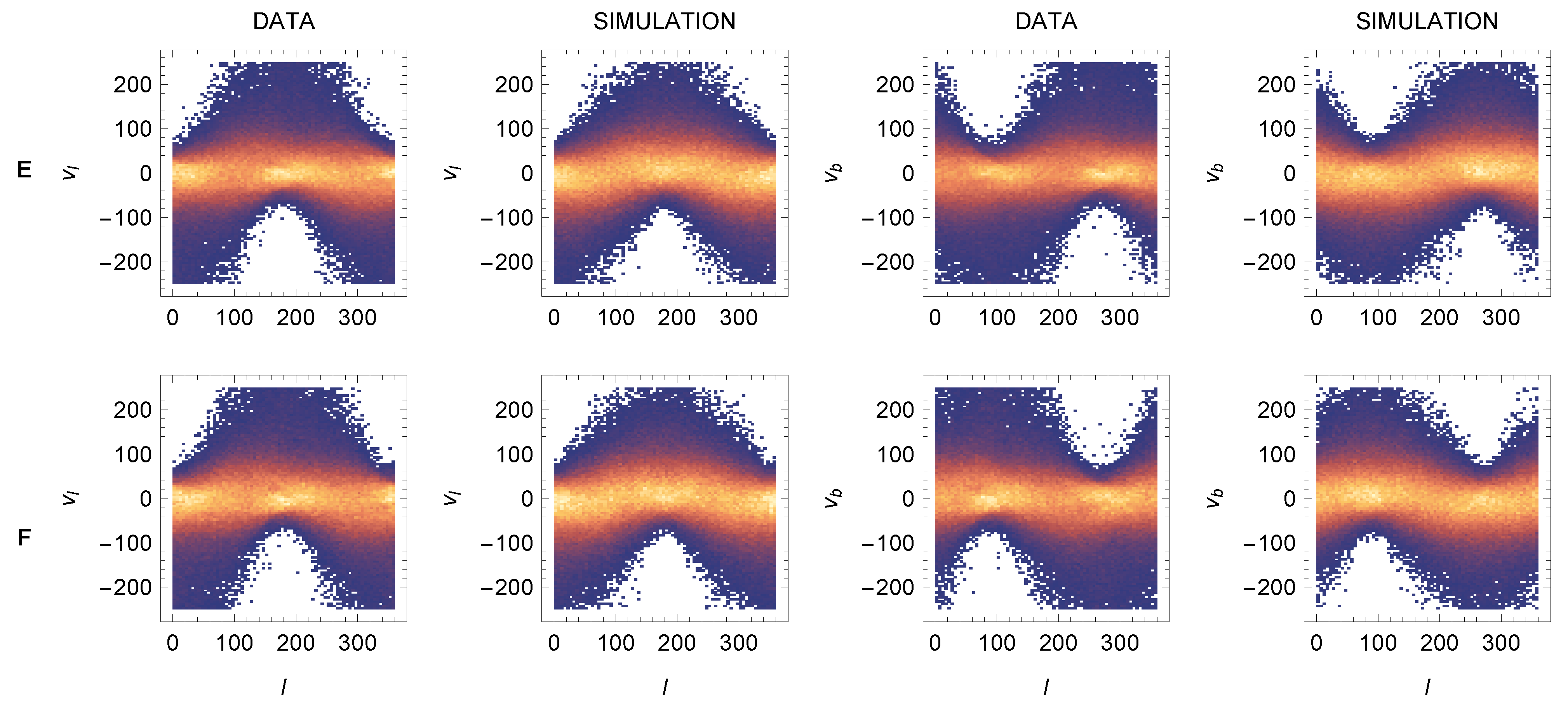
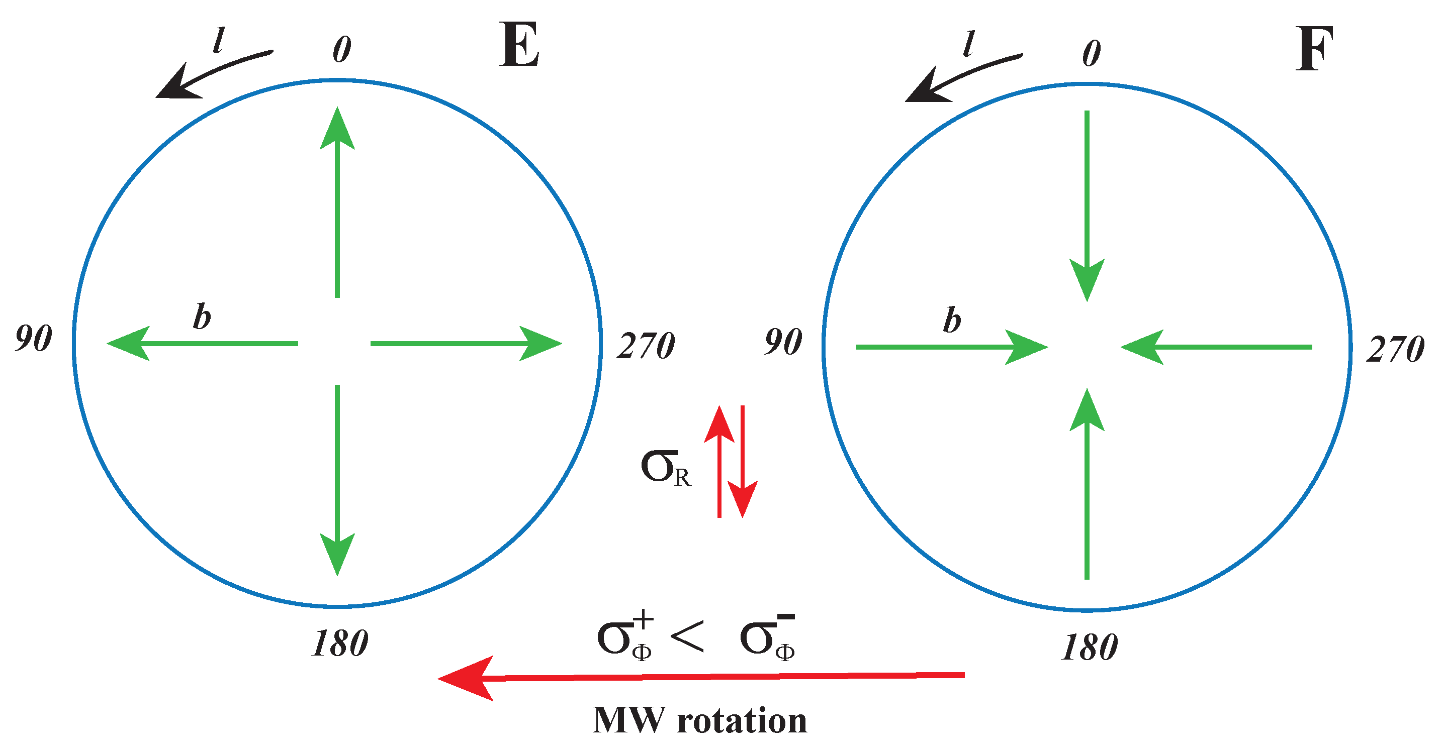
The important result is shown in Figure 15. The asymmetry of histograms $\left(v_l,l\right)$ and $\left(v_b,l\right)$ in sectors E and F with the white areas reflects different projections of the asymmetry represented by Equation (53). The yellow–orange region at $v_l,v_b=0$ corresponds to the peaks in Figure 14E,F, which are the integrals of the histograms over l. The shape of histograms can be explained using Figure 16. Distributions of $v_l$ for $l\approx 0^{\circ },{90}^{\circ },{180}^{\circ },{270}^{\circ }$ are controlled by the parameters ${\sigma }_l^{\pm }$. Their connection with ${\sigma }_{\mathrm{\Phi }}^{\pm }$ and ${\sigma }_R$ can be deduced from the figure. At $l\approx 0^{\circ },$ the directions of $v_l$ and the MW rotation are identical, so ${\sigma }_l^{\pm }\approx {\sigma }_{\mathrm{\Phi }}^{\pm }$. But at $l={180}^{\circ }$, the two directions are opposite, so ${\sigma }_l^{\pm }\approx {\sigma }_{\mathrm{\Phi }}^{\mp }$. At $l\approx {90}^{\circ }\left({270}^{\circ }\right)$, the situation is a little more complicated. If $\left|Z\right|/R$ or $\mathrm{\Theta }$ are small (which is almost our case, see panels E,F in Figure 3, where r$\approx \left|Z\right|$), then the $v_l$ direction can be approximated by vector $\mathbf{R}$, so ${\sigma }_l^{\pm }\approx {\sigma }_R$, similarly for $v_b$ distributions controlled by the parameters ${\sigma }_b^{\pm }$, which are also related to ${\sigma }_{\mathrm{\Phi }}^{\pm }$ and ${\sigma }_R$. Also here, the agreement between the data and the model is very good. Clear evidence for our explanation was provided by the MC simulation: after setting the symmetric ${\sigma }_{\mathrm{\Phi }}^{+}={\sigma }_{\mathrm{\Phi }}^{-}$, the asymmetry in the figure disappears.

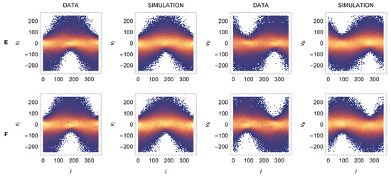
Figure 15. Histograms $\left(v_l,l\right)$ and $\left(v_b,l\right)$ in sectors E and F: data and simulation. Units: l[deg], v[km/s]. Binning $l,v$: $5$deg$,5$ km/s.

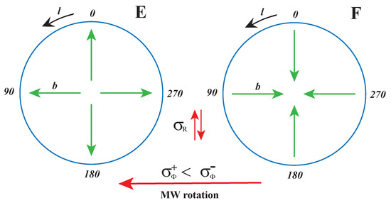
Figure 16. Asymmetry ${\sigma }_{\mathrm{\Phi }}^{+}<{\sigma }_{\mathrm{\Phi }}^{-}$ in the Galactocentric reference frame generates asymmetries in the galactic frame, see text and Figure 15.

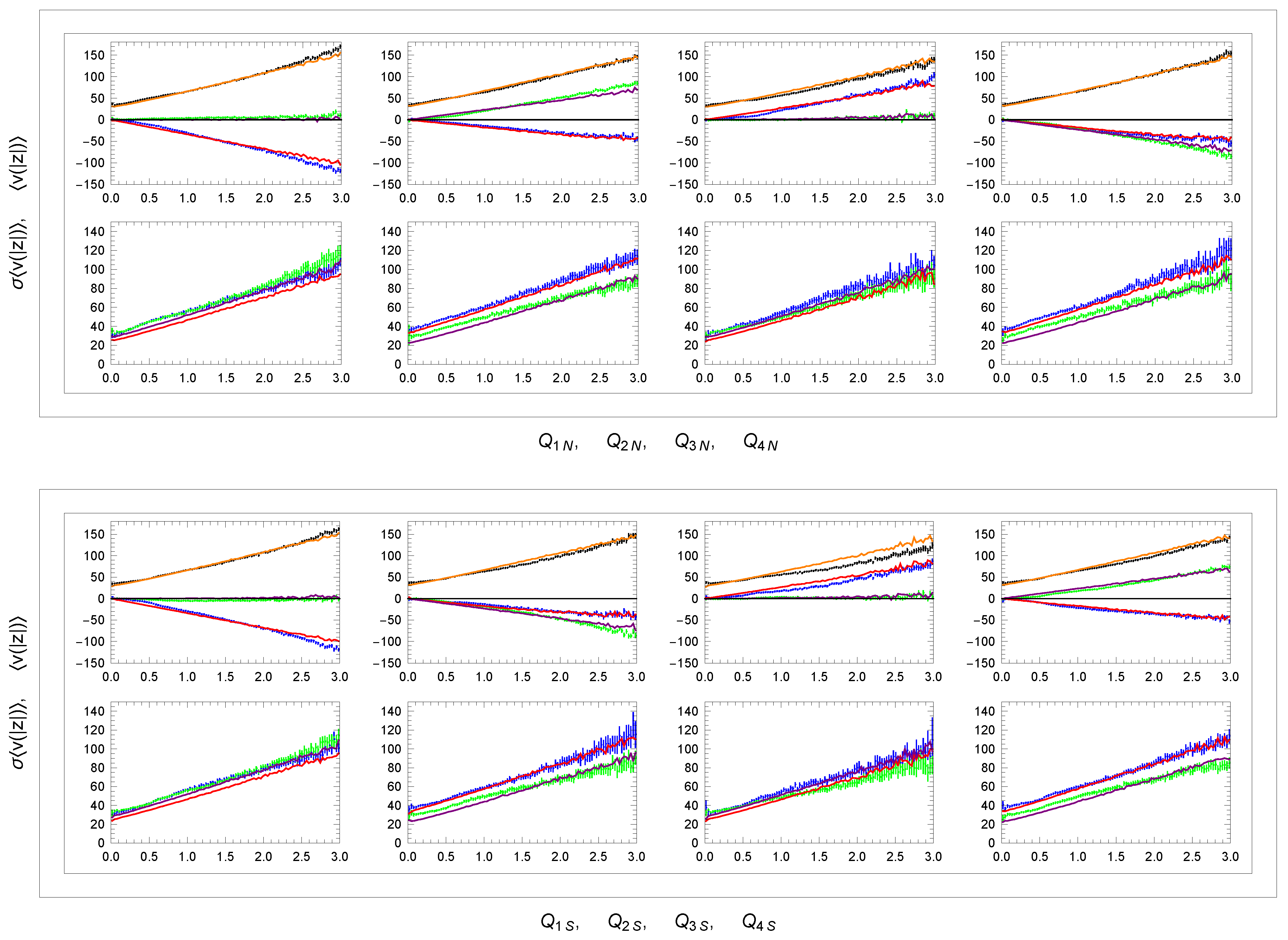
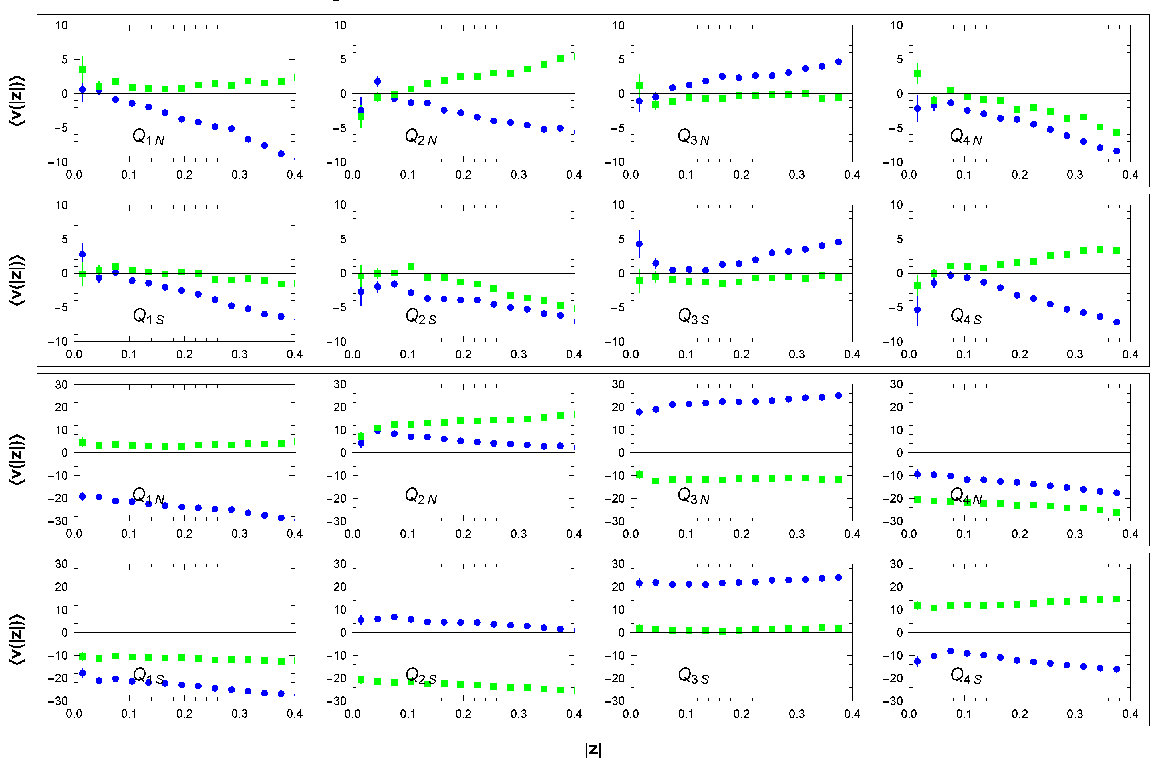
Correct Monte Carlo parameter settings can be verified in wide Q-sectors outside the area of the galactic plane. Figure 17 shows the $z-$dependence of mean values and dispersions of velocity distributions in these sectors. The curves together with the corresponding overall distributions of velocities in broad sectors ${\mathrm{Q}}_{1N}-$ ${\mathrm{Q}}_{4N}$ and ${\mathrm{Q}}_{1S}-$ ${\mathrm{Q}}_{4S}$ in Figure 18 again confirm the very good agreement of the simulation with data. Note in particular the projections $v_l$ in sectors ${\mathrm{Q}}_{1N}$,${\mathrm{Q}}_{3N}$,${\mathrm{Q}}_{1S}$, and ${\mathrm{Q}}_{3S}$ and $v_b$ in sectors ${\mathrm{Q}}_{2N}$,${\mathrm{Q}}_{4N}$,${\mathrm{Q}}_{2S}$, and ${\mathrm{Q}}_{4S}$. This is also due to the asymmetry expressed in Equation (53) that occurs for $\left|Z\right|>0$, as illustrated by the simulated $V_{\mathrm{\Phi }}$ distribution in Figure 13. Note also the expected symmetry between the corresponding ${\mathrm{Q}}_N$ and ${\mathrm{Q}}_S$ panels in Figure 18.

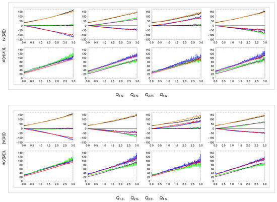
Figure 17. Dependence of mean velocity and its dispersion ($v_l$—blue, $v_b$—green, and $v_{gal}$—black) on distance $\left|z\right|$ in sectors ${\mathrm{Q}}_{1N}$–${\mathrm{Q}}_{4N}$ and ${\mathrm{Q}}_{1S}$–${\mathrm{Q}}_{4S}$: data and simulation model ($v_l$—red, $v_b$—purple, and $v_{gal}$—orange). Units: z[kpc], v[km/s].

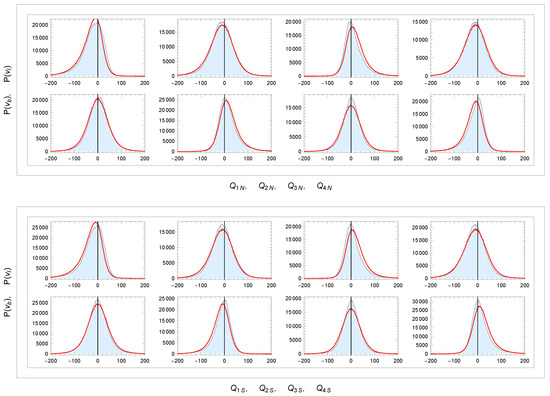
Figure 18. Distributions of $v_l$ and $v_b$ in sectors ${\mathrm{Q}}_{1S}-$${\mathrm{Q}}_{4S}$ and ${\mathrm{Q}}_{1N}-$ ${\mathrm{Q}}_{4N}$: data (light blue) and simulation model (red). Unit: v[km/s]. Binning: 1.6 km/s.

4. Discussion and Conclusions

(1) The results on local Sun’s velocity ${\mathbf{v}}_{\odot }=\left(U_{\odot },V_{\odot },W_{\odot }\right)$, the MW circular velocity $V_c$ and average orbital velocity $V_0$ can be compared with the other measurements presented in Table 2. The excellent agreement with others is obtained for the rotational velocity of the Sun $V_c+V_{\odot }=V_0+\Delta V_{y\odot }$. Within the measurement errors, this result perfectly agrees with all the others, including a very accurate measurement [29]. There is also perfect agreement with the others for $W_{\odot }$ and $V_0$ and a good agreement for $U_{\odot }$. However, differences in $V_c$ and $V_{\odot }$ from different measurements are larger, so our values agree with only some of them (within errors).

Let us add a few remarks on our measurement of $\Delta {\mathbf{V}}_{\odot }$ and $V_0$. Both velocities are obtained independently with the use of a direct and model-independent method. The $\Delta {\mathbf{V}}_{y\odot }$ is measured equally as $\Delta {\mathbf{V}}_{z\odot }$, see Figure 5. For $r_{max}>0.5$ kpc, we obtain a (nearly) constant in the band of small statistical errors. The calculation is based on data from different sectors, so the resulting systematic errors in Table 2 are much larger than the statistical errors. The source of the systematic errors is mainly due to kinematic substructures outside the axial symmetry, which may vary from sector to sector. The correct determination of $\Delta {\mathbf{V}}_{\odot }$ can be verified as follows. At the top half of Figure 19, we show the dependencies of $⟨v\left(z\right)⟩$ (magnified parts of Figure 17) in the eight ${\mathrm{Q}}_{S,N}$ sectors in the LSR reference frame. This frame defines the $\Delta {\mathbf{V}}_{\odot }$ determined from the data in sectors A-D, see Table 2. In these figures, we observe that for $z\to 0$, we have $⟨v_l\left(z\right)⟩,⟨v_b\left(z\right)⟩$$\to 0$, which means that the solar velocity related to the sectors A–D is the same as the velocity related to the nearby stars in all sectors ${\mathrm{Q}}_{S,N}$. This agreement is a simple test that our velocity $\Delta {\mathbf{V}}_{\odot }$ (Equation (36)) is correct. In the bottom half of the figure, we have the same curves for comparison but in a galactic reference frame (the Sun’s rest frame). Note the different scales on the upper and lower parts.

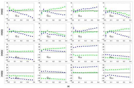
Figure 19. Dependence of mean velocity ($v_l$—blue and $v_b$—green) on distance $|z$ from the galactic plane in sectors ${\mathrm{Q}}_{1N}$–${\mathrm{Q}}_{4N}$ and ${\mathrm{Q}}_{1S}$–${\mathrm{Q}}_{4S}$ in the LSR reference frame (upper part) and the Sun’s rest frame (lower part). Units: z[kpc], v[km/s].

(2) The determination of RC is based on the model-independent definition (15). In Figure 8 and Figure 10, we show RCs measured in different sectors of galactic longitudes. The curves are obtained with very high precision, so as a result, we observe local fluctuations ($\lesssim 10$ km/s) in the structure of the MW rotation. These fluctuations correspond to the velocity substructures and non-axisymmetric kinematic signatures mentioned in Section 1. The fluctuations do not allow us to analyse the RC slope in our limited range of R. Further, we showed that the collective rotation velocity decreases for increasing $\left|Z\right|$, see Figure 11. A similar observation was reported in [21,48]. The slope of the curves is defined in Equation (56) and can be compared with a prediction [50] (Figure 5) of the Besançon model. Within the range of our analysis (0–3 kpc), the average slopes agree very well, although the shape of the curves is slightly different.

(3) Except for observed local fluctuations, the analysed kinematical distributions are very well described by a minimal MW axisymmetric model based on six free parameters in the Galactocentric reference frame. The model describes a simplified scenario in which local velocity fluctuations are averaged. The scale of averaged fluctuations increases with distance from the galactic plane and is defined by the parameters of the model in Table 3. The fluctuations are most significant in the ${\mathbf{N}}_R$ direction, less in the ${\mathbf{N}}_{\mathrm{\Phi }}$ direction, and least in the ${\mathbf{N}}_{\mathrm{\Theta }}$ direction.

The analysis and simulation of kinematical distributions in the studied region that are a part of the MW parameters also need other parameters related to our laboratory: its local 3D velocity $\Delta {\mathbf{V}}_{\odot }$, distance from the galactic centre $R_{\odot }$, and its position $z_{\odot }$ above the galactic plane (neglected). Thus, except for $R_{\odot }$, all the remaining parameters that we obtained in the present analysis are listed in Table 2 and Table 3. For now, we ignore the slope of the RC (Equation (31)), which has in our region a very small effect [6,8]. The model describes the MW rotation as follows.

(a) The rotation is strongly collective in the galactic disk plane with relatively small Gaussian velocity fluctuations ${\sigma }_{\mathrm{\Phi }0},{\sigma }_{\mathrm{\Theta }0},{\sigma }_{R0}$ around the much greater velocity $V_0$. This can be seen in Figure 14 in panels $v_l$ for sectors A and C and panels $v_b$ for sectors A–D. Wider and shifted distributions $v_l$ for sectors B and D are due to the rotation effect shown in Figure 9 and expressed in Equation (43). Our first three parameters are compared with corresponding galactic thin disc parameters obtained in another study, see Table 3. The agreement with [49] is very good.

(b) The parameters ${\sigma }_1$ and ${\sigma }_{\mathrm{\Phi }1}^{-}$ are important outside the galactic plane, where they control the increase in fluctuations with $\left|Z\right|$, as shown in sectors E,F in Figure 12 and the slope of curves in Figure 11. These figures suggest that the collective velocity decreases with increasing $\left|Z\right|$ and the directions of the trajectories are becoming more random and probably less circular. The further effect of ${\sigma }_{\mathrm{\Phi }1}^{-}$ is due to the asymmetry of the distribution $V_{\mathrm{\Phi }}$, which generates the deceleration of collective rotation with increasing $\left|Z\right|$ according to Equation (55). This asymmetry is also manifested very clearly in Figure 15 and Figure 18 (see the comments in the last two paragraphs of Section 3.4).

(c) Our assumption that ${\sigma }_{\mathrm{\Phi }}^{+}$ does not depend on $\left|Z\right|$ can be verified by comparing $v_l$ distributions in the sectors ${\mathrm{Q}}_{1N}$,${\mathrm{Q}}_{3N}$,${\mathrm{Q}}_{1S}$, and ${\mathrm{Q}}_{3S}$ in Figure 18 with the corresponding distributions in sectors A and C in Figure 14. This independence means that in the analysed region,

$$\left|\mathbf{V}\left(R,Z\right)\right|\lesssim V_0+{\sigma }_{\mathrm{\Phi }0}\approx 250\mathrm{km}/\mathrm{s};5\lesssim R\lesssim 13\mathrm{kpc},\left|Z\right|\lesssim 3\mathrm{kpc}.$$

(58)

We showed that the 3D Monte Carlo model fits all studied sectors of the averaged kinematic data very well. Of course, its parameters may require further optimisation in more distant regions.

To conclude, the proposed statistical methods for calculating the local velocity of the Sun, the average rotation velocity $V_0$, and generally the velocity $V_G(R,Z)$ at different positions in the MW can be useful for the analysis of the current and future Gaia data releases. It is always important to be able to compare these parameters obtained by different methods and input data samples. Averaged, axisymmetric approximations of the MW kinematics represented by the Monte Carlo simulation code can be useful in validating axisymmetric dynamic models or determining the scale of local kinematical substructures out of axial symmetry.

References

- Vallenari, A.; Brown, A.G.; Prusti, T.; De Bruijne, J.H.; Arenou, F.; Babusiaux, C.; Biermann, M.; Creevey, O.L.; Ducourant, C.; Evans, D.W.; et al. Gaia Data Release 3: Summary of the content and survey properties. Astron. Astrophys. 2023, 674, A1. [Google Scholar]
- Zavada, P.; Píška, K. Catalog of Wide Binary, Trinary and Quaternary Candidates from the Gaia Data Release 2. Astrophys. J. 2022, 163, 33. [Google Scholar] [CrossRef]
- Antoja, T.; Roca-Fàbrega, S.; De Bruijne, J.; Prusti, T. Kinematics of symmetric Galactic longitudes to probe the spiral arms of the Milky Way with Gaia. Astron. Astrophys. 2016, 589, A13. [Google Scholar] [CrossRef]
- Antoja, T.; Helmi, A.; Romero-Gómez, M.; Katz, D.; Babusiaux, C.; Drimmel, R.; Evans, D.W.; Figueras, F.; Poggio, E.; Reylé, C.; et al. A dynamically young and perturbed Milky Way disk. Nature 2018, 561, 360. [Google Scholar] [CrossRef]
- Bhattacharjee, P.; Chaudhury, S.; Kundu, S. Rotation Curve of the Milky Way out to 200 kpc. Astrophys. J. 2014, 785, 63. [Google Scholar] [CrossRef]
- Eilers, A.C.; Hogg, D.W.; Rix, H.W.; Ness, M.K. The Circular Velocity Curve of the Milky Way from 5 to 25 kpc. Astrophys. J. 2019, 871, 120. [Google Scholar] [CrossRef]
- Mróz, P.; Udalski, A.; Skowron, D.M.; Skowron, J.; Soszyński, I.; Pietrukowicz, P.; Szymański, M.K.; Poleski, R.; Kozłowski, S.; Ulaczyk, K. Rotation Curve of the Milky Way from Classical Cepheids. Astrophys. J. Lett. 2019, 870, 10. [Google Scholar] [CrossRef]
- Reid, M.J.; Menten, K.M.; Brunthaler, A.; Zheng, X.W.; Dame, T.M.; Xu, Y.; Wu, Y.; Zhang, B.; Sanna, A.; Sato, M.; et al. Trigonometric Parallaxes of High Mass Star Forming Regions. Astrophys. J. 2014, 783, 130. [Google Scholar] [CrossRef]
- Burch, B.; Cowsik, R. Properties of Galactic Dark Matter: Constraints from Astronomical Observations. Astrophys. J. 2013, 779, 35. [Google Scholar] [CrossRef]
- Chrobáková, Ž.; López-Corredoira, M.; Labini, F.S.; Wang, H.F.; Nagy, R. Gaia-DR2 extended kinematical maps: III. Rotation curves analysis, dark matter, and MOND tests. Astron. Astrophys. 2020, 642, A95. [Google Scholar] [CrossRef]
- Huang, Y.; Liu, X.W.; Yuan, H.B.; Xiang, M.S.; Zhang, H.W.; Chen, B.Q.; Ren, J.J.; Wang, C.; Zhang, Y.; Hou, Y.H.; et al. The Milky Way’s rotation curve out to 100 kpc and its constraint on the Galactic mass. Mon. Not. R. Astron. Soc. 2016, 463, 2623. [Google Scholar] [CrossRef]
- Jiao, Y.; Hammer, F.; Wang, J.L.; Yang, Y.B. Which Milky Way masses are consistent with the slightly declining 5–25 kpc rotation curve? Astron. Astrophys. 2021, 654, A25. [Google Scholar] [CrossRef]
- Wegg, C.; Gerhard, O.; Bieth, M. The gravitational force field of the Galaxy measured from the kinematics of RR Lyrae in Gaia. Mon. Not. R. Astron. Soc. 2019, 485, 3296. [Google Scholar] [CrossRef]
- Ablimit, I.; Zhao, G. The Milky Way’s Circular Velocity Curve and Its Constraint on the Galactic Mass with RR Lyrae Stars. Astrophys. J. 2017, 846, 10. [Google Scholar] [CrossRef]
- Sofue, Y. Rotation Curve of the Milky Way and the Dark Matter Density. Galaxies 2020, 8, 37. [Google Scholar] [CrossRef]
- Drimmel, R.; Romero-Gómez, M.; Chemin, L.; Ramos, P.; Poggio, E.; Ripepi, V.; Andrae, R.; Blomme, R.; Cantat-Gaudin, T.; Castro-Ginard, A.; et al. Gaia Data Release 3: Mapping the asymmetric disc of the Milky Way. Astron. Astrophys. 2023, 674, A37. [Google Scholar]
- Katz, D.; Antoja, T.; Romero-Gómez, M.; Drimmel, R.; Reylé, C.; Seabroke, G.M.; Soubiran, C.; Babusiaux, C.; Di Matteo, P.; Figueras, F.; et al. Gaia Data Release 2: Mapping the Milky Way disc kinematics. Astron. Astrophys. 2018, 616, A11. [Google Scholar]
- Kawata, D.; Baba, J.; Ciucă, I.; Cropper, M.; Grand, R.J.; Hunt, J.A.; Seabroke, G. Radial distribution of stellar motions in Gaia DR2. MNRAS Lett. 2018, 479, 108. [Google Scholar] [CrossRef]
- López-Corredoira, M.; Sylos Labini, F. Gaia-DR2 extended kinematical maps. Astron. Astrophys. 2019, 621, A48. [Google Scholar] [CrossRef]
- Ramos, P.; Antoja, T.; Figueras, F. Riding the kinematic waves in the Milky Way disk with Gaia. Astron. Astrophys. 2018, 619, A72. [Google Scholar] [CrossRef]
- Wang, H.F.; Chrobáková, Ž.; López-Corredoira, M.; Labini, F.S. Mapping the Milky Way Disk with Gaia DR3. Astrophys. J. 2023, 942, 12. [Google Scholar] [CrossRef]
- Wang, H.F.; López-Corredoira, M.; Huang, Y.; Carlin, J.L.; Chen, B.Q.; Wang, C.; Chang, J.; Zhang, H.W.; Xiang, M.S.; Yuan, H.B.; et al. Mapping the Galactic disc with the LAMOST and Gaia red clump sample: II. 3D asymmetrical kinematics of mono-age populations in the disc between 6–14 kpc. Mon. Not. R. Astron. Soc. 2020, 491, 2104. [Google Scholar] [CrossRef]
- Kushniruk, I.; Schirmer, T.; Bensby, T. Kinematic structures of the solar neighbourhood revealed by Gaia DR1/TGAS and RAVE. Astron. Astrophys. 2017, 608, A73. [Google Scholar] [CrossRef]
- Kawata, D.; Bovy, J.; Matsunaga, N.; Baba, J. Galactic rotation from Cepheids with Gaia DR2 and effects of non-axisymmetry. Mon. Not. R. Astron. Soc. 2019, 482, 40. [Google Scholar] [CrossRef]
- Tian, H.J.; Liu, C.; Wan, J.C.; Wang, Y.G.; Wang, Q.; Deng, L.C.; Cao, Z.H.; Hou, Y.H.; Wang, Y.F.; Wu, Y.; et al. Peculiar in-plane velocities in the outer disc of the Milky Way. Res. Astron. Astrophys. 2017, 17, 114. [Google Scholar] [CrossRef]
- Bland-Hawthorn, J.; Gerhard, O. The Galaxy in Context: Structural, Kinematic, and Integrated Properties. Annu. Rev. Astron. Astrophys. 2016, 54, 529. [Google Scholar] [CrossRef]
- Antoja, T.; De Bruijne, J.; Figueras, F.; Mor, R.; Prusti, T.; Roca-Fàbrega, S. The intricate Galaxy disk: Velocity asymmetries in Gaia-TGAS. Astron. Astrophys. 2017, 602, L13. [Google Scholar] [CrossRef][Green Version]
- Mikkola, D.; Paul, J.; McMillan, P.; Hobbs, D. New stellar velocity substructures from Gaia DR3 proper motions. Mon. Not. R. Astron. Soc. 2023, 519, 1989. [Google Scholar] [CrossRef]
- Abuter, R.; Amorim, A.; Bauböck, M.; Berger, J.P.; Bonnet, H.; Brandner, W.; Clénet, Y.; Du Foresto, V.C.; De Zeeuw, P.T.; Dexter, J.; et al. A geometric distance measurement to the Galactic center black hole with 0.3% uncertainty. Astron. Astrophys. 2019, 625, L10. [Google Scholar]
- Bennet, M.; Bovy, J. Vertical waves in the solar neighbourhood in Gaia DR2. Mon. Not. R. Astron. Soc. 2019, 482, 1417. [Google Scholar] [CrossRef]
- Schönrich, R.; Binney, J.; Dehnen, W. Local kinematics and the local standard of rest. Mon. Not. R. Astron. Soc. 2010, 403, 1829. [Google Scholar] [CrossRef]
- Gaia Data Processing and Analysis Consortium 2023, Gaia Data Release 3, Documentation Release 1.3. Available online: https://gea.esac.esa.int/archive/documentation/GDR3/ (accessed on 20 January 2025).
- Antoja, T.; McMillan, P.J.; Kordopatis, G.; Ramos, P.; Helmi, A.; Balbinot, E.; Cantat-Gaudin, T.; Chemin, L.; Figueras, F.; Jordi, C.; et al. Gaia Early Data Release 3: The Galactic anticentre. Astron. Astrophys. 2021, 649, A8. [Google Scholar]
- Bailer-Jones, C.A.L. Estimating Distances from Parallaxes. Publ. Astron. Soc. Pac. 2015, 127, 994–1009. [Google Scholar] [CrossRef]
- Gaia Collaboration: Luri, X.; Brown, A.G.A.; Sarro, L.M. Gaia Data Release 2: Using Gaia parallaxes. Astron. Astrophys. 2018, 616, A9. [Google Scholar] [CrossRef]
- Lindegren, L.; Bastian, U.; Biermann, M.; Bombrun, A.; De Torres, A.; Gerlach, E.; Geyer, R.; Hernández, J.; Hilger, T.; Hobbs, D.; et al. Gaia Early Data Release 3: Parallax bias versus magnitude, colour, and position. Astron. Astrophys. 2021, 649, A4. [Google Scholar] [CrossRef]
- Jeans, J.H. On the theory of star-streaming and the structure of the universe. Mon. Not. R. Astron. Soc. 1915, 76, 70. [Google Scholar] [CrossRef]
- Bovy, J. Dynamics and Astrophysics of Galaxies; Princeton University Press: Princeton, NJ, USA, 2024; (in preparation). Available online: https://galaxiesbook.org/index.html (accessed on 20 January 2025).
- Li, X.; Yang, P.; Wang, H.F.; Li, Q.; Luo, Y.P.; Luo, Z.Q.; Wang, G.Y. Asymmetric Drift Map of the Milky Way disk Populations between 8–16 kpc with LAMOST and Gaia datasets. arXiv 2023, arXiv:2310.01311. [Google Scholar] [CrossRef]
- Bobylev, V.V.; Bajkova, A.T. Kinematic Analysis of Solar-Neighborhood Stars Based on RAVE4 Data. Astron. Lett. 2016, 42, 90. [Google Scholar] [CrossRef]
- Tian, H.J.; Liu, C.; Carlin, J.L.; Zhao, Y.H.; Chen, X.L.; Wu, Y.; Li, G.W.; Hou, Y.H.; Zhang, Y. The Stellar Kinematics in the Solar Neighborhood from LAMOST Data. Astrophys. J. 2015, 809, 145. [Google Scholar] [CrossRef]
- Dehnen, W.; James, J. Binney, J.J. Local stellar kinematics from Hipparcos data. Mon. Not. R. Astron. Soc. 1998, 298, 387. [Google Scholar] [CrossRef]
- Bovy, J.; Prieto, C.A.; Beers, T.C.; Bizyaev, D.; Da Costa, L.N.; Cunha, K.; Ebelke, G.L.; Eisenstein, D.J.; Frinchaboy, P.M.; Pérez, A.E.; et al. The Milky Way’s circular velocity curve between 4 and 14 kpc from APOGEE data. Astrophys. J. 2012, 759, 131. [Google Scholar] [CrossRef]
- Bovy, J.; Bird, J.C.; Pérez, A.E.; Majewski, S.R.; Nidever, D.L.; Zasowski, G. The Power Spectrum of the Milky Way: Velocity Fluctuations in the Galactic Disk. Astrophys. J. 2015, 800, 83. [Google Scholar] [CrossRef]
- Schönrich, R. Galactic rotation and solar motion from stellar kinematics. Mon. Not. R. Astron. Soc. 2012, 427, 274. [Google Scholar] [CrossRef]
- Koposov, S.E.; Rix, H.-W.; Hogg, D.W. Constraining the Milky Way potential with a 6-D phase-space map of the GD-1 stellar stream. Astrophys. J. 2010, 712, 260. [Google Scholar] [CrossRef]
- Hayes, C.R.; Law, D.R.; Majewski, S.R. Constraining the Solar Galactic Reflex Velocity using Gaia Observations of the Sagittarius. Astrophys. J. Lett. 2018, 867, L20. [Google Scholar] [CrossRef]
- Anguiano, B.; Majewski, S.R.; Hayes, C.R.; Prieto, C.A.; Cheng, X.; Bidin, C.M.; Beaton, R.L.; Beers, T.C.; Minniti, D. The Stellar Velocity Distribution Function in the Milky Way Galaxy. Astron. J. 2020, 160, 43. [Google Scholar] [CrossRef]
- Vieira, K.; Carraro, G.; Korchagin, V.; Lutsenko, A.; Girard, T.M.; van Altena, W. Milky Way Thin and Thick Disk Kinematics with Gaia EDR3 and RAVE DR5. Astrophys. J. 2022, 932, 28. [Google Scholar] [CrossRef]
- Bienaymé, O.; Leca, J.; Robin, A.C. A new dynamically self-consistent version of the Besançon Galaxy model. Astron. Astrophys. 2018, 620, A103. [Google Scholar] [CrossRef]
Disclaimer/Publisher’s Note: The statements, opinions and data contained in all publications are solely those of the individual author(s) and contributor(s) and not of MDPI and/or the editor(s). MDPI and/or the editor(s) disclaim responsibility for any injury to people or property resulting from any ideas, methods, instructions or products referred to in the content. |
© 2025 by the authors. Licensee MDPI, Basel, Switzerland. This article is an open access article distributed under the terms and conditions of the Creative Commons Attribution (CC BY) license (https://creativecommons.org/licenses/by/4.0/).