An Improved Search and Rescue Algorithm for Global Optimization and Blood Cell Image Segmentation

Abstract

Image segmentation has been one of the most active research areas in the last decade. The traditional multi-level thresholding techniques are effective for bi-level thresholding because of their resilience, simplicity, accuracy, and low convergence time, but these traditional techniques are not effective in determining the optimal multi-level thresholding for image segmentation. Therefore, an efficient version of the search and rescue optimization algorithm (SAR) based on opposition-based learning (OBL) is proposed in this paper to segment blood-cell images and solve problems of multi-level thresholding. The SAR algorithm is one of the most popular meta-heuristic algorithms (MHs) that mimics humans’ exploration behavior during search and rescue operations. The SAR algorithm, which utilizes the OBL technique to enhance the algorithm’s ability to jump out of the local optimum and enhance its search efficiency, is termed mSAR. A set of experiments is applied to evaluate the performance of mSAR, solve the problem of multi-level thresholding for image segmentation, and demonstrate the impact of combining the OBL technique with the original SAR for improving solution quality and accelerating convergence speed. The effectiveness of the proposed mSAR is evaluated against other competing algorithms, including the L’evy flight distribution (LFD), Harris hawks optimization (HHO), sine cosine algorithm (SCA), equilibrium optimizer (EO), gravitational search algorithm (GSA), arithmetic optimization algorithm (AOA), and the original SAR. Furthermore, a set of experiments for multi-level thresholding image segmentation is performed to prove the superiority of the proposed mSAR using fuzzy entropy and the Otsu method as two objective functions over a set of benchmark images with different numbers of thresholds based on a set of evaluation matrices. Finally, analysis of the experiments’ outcomes indicates that the mSAR algorithm is highly efficient in terms of the quality of the segmented image and feature conservation, compared with the other competing algorithms.

1. Introduction

Image thresholding is a popular operation used in computer vision to process and analyze images in fields such as medicine, engineering, agriculture, and manufacturing. It is most commonly used in image segmentation to provide accurate feature extraction in biological image processing, pattern recognition, and robotic vision [1]. Thresholding is one of the most important main segmentation steps that has proven effective in different applications [2,3]. The main goal of image thresholding is to obtain optimal threshold values from the image, for which the image histogram is used. The histogram is a vital step in the segmentation methods for defining the probability distribution value of pixels in the image [4]. The thresholding technique can be classified into two different groups: multi-level and bi-level thresholding. Multi-level thresholding usins two or more thresholding values to split an image into many different groups, while bi-level thresholding uses one threshold value to split an image into two groups [5,6].

Recently, many researchers have illustrated the capability of MHs to solve a diversity of complex optimization problems in different fields, such as biomedical [7], engineering [8,9], medical [10,11], communications [12], image segmentation [13], and feature selection [14]. MHs are considered flexible, non-derived, and highly clever in obtaining an optimal solution. Furthermore, these algorithms are considered the best method for providing the best solutions for complex optimization problems with the latest developments in computer techniques. Due to their advantages, MHs have become widely utilized to realize the optimal thresholds of color and gray-level images. MHs applied the search procedure to a problem landscape with a set of search agents that act as candidate solutions created repeatedly in an iterative procedure using heuristic operators. These operators, when utilized in various orders, generate different search strategies. In the same context, MHs are classified into four main groups: swarm-based algorithms, natural evolution-based algorithms, human-based algorithms, and physics-based algorithms [15,16].

As per published researches on swarm-based algorithms (SA), SA mimics the behavior of an organism within groups. Organisms usually interact with one another to achieve the best collective behavior [17]. Some works published in these offshoots, such as particle swarm optimization (PSO) [18], mimic the hunting behavior of birds and fish swarms. The natural evolution-based algorithms imitate biological evolution processes such as recombination, crossover, mutation, and feature inheritance in offspring [19]. The fitness function determines the quality of candidate solutions to the optimization problems, which work as individuals in a population. The genetic algorithm (GA) [20] and differential evolution (DE) [21] are two evolutionary algorithms inspired by biological evolution. The third category of MHs is human-based algorithms that mimic gregarious human attitudes. Many algorithms belong to these branches, such as the heap-based optimizer (HBO) [22], election campaign algorithm (ECA) [23], and teaching–learning-based optimization (TLBO) [24]. The fourth category of MHs is called physics-based algorithms, and these are inspired by physics to create factors that allow for the search of the best solution within the search scope. Many algorithms have been published in this branch, such as the electromagnetism-based algorithms (EMO) [25] and the GSA algorithm [26].

In the literature, several theories have been proposed to explain the efficacy of MHs on image thresholding [27,28]. There are several examples of MHs in this field; nevertheless, the following are a few notable state-of-the-art research efforts. In [29], the moth-swarm algorithm (MSA) was used to determine the optimal threshold values with the Kapur method. Additionally, ant colony optimization (ACO) in [30] is utilized in image segmentation based on a non-local 2D histogram and Kapur’s entropy as object functions with the multi-threshold image segmentation (MTH) method. In [31], researchers used the Otsu and Kapur methods with a modified firefly algorithm to process images. In the same context, three new versions of the manta ray foraging optimization algorithm and the chimp optimization algorithm (ChOA) have been proposed to tackle the image segmentation problem using multi-level thresholding [32,33,34]. The researchers in [35] used (MTH) image segmentation with a novel concept of MHs called hyper-heuristics, in which each iteration defined the best execution sequence of MHs to determine the best thresholds. In [27], the black widow optimization (BWO) algorithm used Otsu or Kapur techniques as an objective function with multi-level thresholding to determine the optimal thresholding value in the gray level. An efficient krill herd (EKH) algorithm in [36] was utilized to determine the best thresholding values at different levels for color images, with Kapur’s entropy, Tsallis entropy, and the Otsu methods. The HHO algorithm is the novel algorithm in [37], and the hybridization of HHO is accomplished by adding another efficient algorithm, the DE algorithm, which together is termed HHO-DE. In particular, the entire population is divided into two equal subpopulations that will be assigned to the DE and HHO algorithms, respectively, and this hybridization used Otsu and Kapur’s methods as the objective functions.

Regardless of the previous optimization methods, SAR [38] is also used to determine the optimal multi-level thresholding for image segmentation. In terms of efficiency and simplicity, the SAR outperforms several other biologically inspired procedures as a competitive and modern population-based optimization technique. It mimics the exploration behavior of humans during search and rescue operations. The researchers [38] have proven that SAR performs better in terms of stability and accuracy when compared with other optimization techniques when tested on standard benchmark functions.

Many of the MHs used to solve various optimization problems in the literature, such as a lack of global search capability, early conversion, or trapping in local regions. This gives researchers a yardstick to propose hybrid and modified versions. Many researchers use OBL to improve the search efficiency of MHs [39]. Tizhoosh released the first version of OBL in 2005 [40], and MHs have used it in a variety of ways to improve exploratory searchability. The researchers improved the elephant herding optimization (EHO) using dynamic Cauchy mutation (DCM) and OBL learning for solving multi-thresholding problems [41]. DCM healed premature convergence, and OBL resolved slow convergence in EHO, according to the authors. This study utilized Otsu and Kapur’s methods as two fitness functions to determine threshold values for image segmentation. In [42], the marine predator algorithm (MPA) is improved using OBL (MPA-OBL) for enhancing convergence and search efficiency and solving the IEEE CEC’2020 benchmark problems. MPA-OBL used Kapur’s and the Otsu methods as two fitness functions with a diversity of benchmark images at different thresholds.

In spite of some studies related to MHs and OBL to solving image thresholding problems, it is difficult to find more research related to relevant literature. Nevertheless, OBL-based MHs are often applied to different optimization problems. As a result, the purpose of this study is to deepen the research in the image segmentation field by employing the most recent SAR; in reality, this is the first instance of SAR implemented on the image segmentation and CEC’2020 benchmark functions. SAR was introduced in July 2020 to mimic the exploration behavior of humans during search and rescue operations, which outperformed a huge number of well-known counterparts on a variety of engineering and mathematics benchmark problems. Despite the efficacy of SAR’s search mechanisms, there are some fields where it may be enhanced further to prove its efficiency on various optimization problems, such as image thresholding problems, because the algorithm may miss some critical search regions. To solve this problem, we combined the SAR algorithm with OBL (SAR-OBL) to generate solutions from potential regions for exploring search space more rigorously. More crucially, we enhance its local search capability by utilizing solutions generated from the surrounding promising regions to avoid the trap of local optima. As a result, the proposed SAR diversity comes with a trade-off balance between exploration and exploitation. We evaluate the proposed SAR-OBL on CEC’2020 benchmark functions before it is used to solve multi-level image thresholding problems.

The main goal of this paper is to enable researchers to use a novel metaheuristic algorithm with opposition-based learning (OBL) to increase the performance of image segmentation in the medical field. Furthermore, this paper aims to discuss the benefits and downsides of the mSAR algorithm in image segmentation. Finally, the main contributions of this paper can be summarized as follows:

• An improved opposition-based search and rescue optimization algorithm (mSAR) is presented.
• The search efficiency and convergence of mSAR have been improved.
• Fuzzy entropy and the Otsu method are applied.

The paper is structured as follows: in Section 2, the SAR algorithm and OBL search strategy will be discussed. Section 2.3 is devoted to a mathematical model of fuzzy entropy and Otsu methods. Section 3 presents the proposed algorithm. The evaluation of SAR-OBL is presented in Section 4. The experimental results are discussed and analyzed in Section 5. The conclusion is reported in Section 6.

2. Preliminaries

This section studies the inspiration of the SAR algorithm and its mathematical model and discusses the OBL strategy.

2.1. Search and Rescue Optimization Algorithm

The mathematical model of the SAR algorithm is discussed in this section. Search and rescue operations are one type of group exploration. A search is a methodical operation that employs resources and available personnel to identify the individuals involved in the ordeal. A rescue operation seeks to recover people who are in danger and transport them to a safe location. Humans search in groups, and each searching group regulates its practice to be ready for its respective operations. Based on their training, humans can find clues and traces of missing people. The found clues are of varying value and contain varying amounts of information regarding the missing individuals. For example, some clues refer to the probability of the presence of lost individuals in that area. The clues are evaluated by each group member depending on his or her training. This evaluation delivers information about the found clues to other members via communication equipment. Last but not least, they search based on the information gleaned from them and the significance of these hints. Social and individual stages are the main stages in search and rescue operations. In the social stage, searching is based on the location of found clues and their importance, while in the individual stage, the search is executed regardless of the importance of clues. Clues can be divided into two types: hold clues and abandoned clues.

2.1.1. The Clues

The positions of the left clues are saved in a memory matrix X in the model we proposed, while the positions of the humans are saved in a position matrix Y. The dimensions of matrix X are the same as those of matrix Y. They are $M\times N$ matrices, where M is the number of the members of the group and N refers to the problems’ dimension. The clues matrix Z contains the locations of the discovered clues, and it is composed of matrices Y and X. Most new solutions in individual and social stages are introduced dependent on the clue matrix, and this is a primary part of SAR. Equation (1) presents the clue matrix Z and matrices X, Y, and Z are upgraded in each of the human search stages.

$$\mathrm{Z}=\left[\begin{array}{c}Y\hfill \\ X\hfill \end{array}\right]=\left[\begin{array}{ccc}{Y}_{11}\hfill & \cdots \hfill & Y1N\hfill \\ ⋮\hfill & \ddots \hfill & ⋮\hfill \\ Y_{M1}\hfill & \cdots \hfill & Y_{MN}\hfill \\ X_{11}\hfill & \cdots \hfill & X_{1N}\hfill \\ ⋮\hfill & \ddots \hfill & ⋮\hfill \\ X_{M1}\hfill & \cdots \hfill & X_{MN}\hfill \end{array}\right],$$

(1)

where Y and X are human locations and memory matrices, respectively, and $Y_{M1}$ is the first dimension location for human Mth. Furthermore, the first memory’s Nth dimension is located at $X_{1N}$. The two stages of human search are modeled in the following section.

2.1.2. Social and Individual Stages

According to the preceding explications, Equation (2) is utilized to determine the search direction.

$$S{D}_k=\left(Y_k-Z_j\right),j\ne k$$

(2)

where the location of the jth clue, the location of the kth human, and the search direction for the kth human are $Z_j$, $Y_k$, and $S{D}_k$, respectively. j is a random parameter inside (1, 2M). For $k=j,Z_k$ will be equal to $Y_k$. Thus, j is elected in such a way that $j\ne k$. The social phase can be implemented by Equation (3).

$$Y_{j,i}^{\prime }=\left\{\begin{array}{c}\left\{\begin{array}{cc}{Z}_{k,i}+\mathrm{r}1\times \left(X_{j,i}-Z_{k,i}\right)& \mathrm{if}f\left(Z_k\right)>f\left(X_j\right)\\ X_{j,i}+\mathrm{r}1\times \left(X_{j,i}-Z_{k,i}\right)& \mathrm{otherwise}\end{array}\right.\\ X_{j,i}& \mathrm{if}r2<SE\mathrm{or}i=i_{\mathrm{rand}}i=1,\cdots ,N\end{array}\right.,$$

(3)

where the location of the ith dimension for the jth human is $Y_{j,i}^{\prime }$. The new location of the ith dimension for the kth clue is $Z_{k,i}$. The fitness function values for the solution ${\mathbf{X}}_{\mathbf{j}}$ and ${\mathbf{Z}}_{\mathbf{k}}$ are $f\left(X_j\right)$ and $f\left(Z_k\right)$, respectively. $r1$ is a random parameter inside $[-1,1]$, $r2$ and $SE$ are a distributed random parameters inside range $[0,1]$. $i_{\mathrm{rand}}$ is a random parameter inside range 1 and N which used to ensure that at least one dimension of $Y_{j,i}^{\prime }$ is different from $X_{j,i}$. Equation (3) shows the new location of the jth human in all dimensions.

The individual stage used Equation (4) to determine the new location of the jth human.

$$Y_j^{\prime }=X_j+r3\times \left(C_k-C_m\right),j\ne k\ne m.$$

(4)

where k, m are random values ranging between 1 and $2N$. This way, $j\ne k\ne m$ was employed for choosing k and m to prevent moving along other clues. $r3$ is a random value with a uniform distribution inside the range $[0,1]$. Equation (5) is used to modify the new location of the jth human.

$$Y_{j,i}^{\prime }=\left\{\begin{array}{cc}\left(X_{j,i}+X_i^{max}\right)/2\hfill & \mathrm{if}{X}_{j,i}^{\prime }>X_i^{max}\hfill \\ \left(X_{j,i}+X_i^{min}\right)/2\hfill & \mathrm{if}{X}_{j,i}^{\prime }<X_i^{min}\hfill \end{array},i=1,\cdots ,N\right.,$$

(5)

where $X_i^{\min }$, $X_i^{max}$ are the values of the minimum and maximum threshold for ith dimension, respectively.

2.1.3. Update Locations and Information

Members of the group will search according to these two stages in each iteration, and if the value of the fitness function after each stage in the first location is $\left(f\left(X_j\right)\right)$ less than the second location $Y_j^{\prime }\left(f\left(Y_j^{\prime }\right)\right)$. The first location $\left(X_j\right)$ will be saved in a random location of the memory matrix (M).

$$M_n=\left\{\begin{array}{cc}{X}_j\hfill & \mathrm{if}f\left(Y_j^{\prime }\right)>f\left(X_j\right)\hfill \\ M_n\hfill & \mathrm{otherwise}\hfill \end{array}\right.,$$

(6)

$$X_j=\left\{\begin{array}{cc}{Y}_j^{\prime }\hfill & \mathrm{if}f\left(Y_j^{\prime }\right)>f\left(X_j\right)\hfill \\ X_j\hfill & \mathrm{otherwise}\hfill \end{array}\right.,$$

(7)

where $M_n$ indicates the location of the nth saved clue in the memory matrix and the random value ranged between 1 and N is n.

2.1.4. Constraint-Handling Strategies

The penalty functions strategy, the $\epsilon$-constrained method, and stochastic ordering are all methods for dealing with constraints. The $\epsilon$-constrained method is one of the prevalent constraint-handling methods used in this study. According to this strategy, for a maximizing problem, this technique considers one solution to be better than another solution if the following requirements are satisfied:

$$X_2\mathrm{is}\mathrm{better}\mathrm{than}{X}_1:\left\{\begin{array}{cc}f\left(X_2\right)>f\left(X_1\right)\hfill & \mathrm{if}G\left(X_2\right)\le \epsilon \mathrm{and}G\left(X_1\right)\le \epsilon \hfill \\ f\left(X_2\right)>f\left(X_1\right)\hfill & \mathrm{if}G\left(X_2\right)=G\left(X_1\right)\hfill \\ G\left(X_2\right)<G\left(X_1\right)\hfill & \mathrm{otherwise}\hfill \end{array}\right..$$

(8)

The parameter $\epsilon$ is used to control the size of feasible space and this parameter can be calculated by Equation (8).

The SAR algorithm is compared using the $\epsilon$-constrained technique for constraint optimization problems. Thus, Equations (3), (6) and (7) are updated as follows:

$$Y_{j,i}^{\prime }=\left\{\begin{array}{c}\left\{\begin{array}{cc}{Z}_{k,i}+\mathrm{r}1\times \left(X_{j,i}-Z_{k,i}\right)& \mathrm{if}f\left(Z_k\right)\mathrm{is}\mathrm{better}\mathrm{than}f\left(X_j\right)\\ X_{j,i}+\mathrm{r}1\times \left(X_{j,i}-Z_{k,i}\right)& \mathrm{otherwise}\end{array}\right.\\ X_{j,i}& \mathrm{if}r2<SE\mathrm{or}i=i_{\mathrm{rand}}i=1,\cdots ,N\end{array}\right.,$$

(9)

$$M_n=\left\{\begin{array}{cc}{Y}_j^{\prime }\hfill & \mathrm{if}{Y}_j^{\prime }\mathrm{is}\mathrm{better}\mathrm{than}{X}_j\hfill \\ M_n\hfill & \mathrm{otherwise}\hfill \end{array}\right.,$$

(10)

$$X_j=\left\{\begin{array}{cc}{Y}_j^{\prime }\hfill & \mathrm{if}{Y}_j^{\prime }\mathrm{is}\mathrm{better}\mathrm{than}{X}_j\hfill \\ X_j\hfill & \mathrm{otherwise}\hfill \end{array}\right.,$$

(11)

where $Z_k$ or $Y_j^{\prime }$ are better than $X_j$ if and only if Equation (8) is satisfied.

2.2. Opposition-Based Learning

OBL is a new mechanism in computational intelligence, and the main principle of OBL is to enhance the efficiency of the optimization OBL of MHs [42]. HR. Tizhoosh [40] introduced the OBL. Many researchers use OBL to enhance the quality of their population-initiated solutions by diversifying these solutions. In general, in MHs, when the initial solutions are near the optimal location, convergence occurs quickly; moreover, late convergence is expected. In this case, the OBL technique provides additional solutions by taking into account opposite search regions that may be near the global optimum. For understanding the definition of OBL, the opposite point of P is computed by:

$${\overrightarrow{z}}_j=\left({\overrightarrow{ub}}_j+{\overrightarrow{lb}}_j\right)-{\overrightarrow{z}}_j,$$

(12)

where $ub$ and $lb$ are upper and lower bounds for the jth component of a vector z.

Previous studies indicate that researchers in the MH community have predominantly used various MHs. For instance, in [43], the HHO algorithm used the OBL strategy to enhance the search efficiency of the algorithm. While the researchers in [44] presented a new version of SCA based on OBL, this version is designed to jump out of local optima during the search processes. An improved whale optimization algorithm (WOA) is developed in [45] by combining the OBL and DE algorithms for improving exploration and exploitation by generating opposite values. In [46], researchers used OBL to improve the grasshopper optimization algorithm to solve engineering problems and benchmark functions. The EO algorithm used OBL and a set of novel update rules in [47] for modifying the EO, and this modification is called m-EO. The shuffled frog-leaping algorithm (SFLA) used the OBL to improve SFLA in [48], where OBL is combined into the memeplexes before the frog initiates foraging. In [49], researchers combine OBL with an enhanced scatter search (eSS) for large-scale parameter estimation in kinetic models of medical fields. According to this research work, OBL is employed only during the initiation phase for improving the rate of convergence and avoiding tumbling into the local optima of SAR. After that, mSAR is utilized for solving the problem of multi-thresholding for image segmentation using fuzzy entropy and the Otsu variance as objective functions.

2.3. Image Thresholding Methods

In this subsection, the mathematical model of two object functions used in image thresholding is explained, and these object functions are fuzzy entropy [50] and Otsu variance [51].

2.3.1. Fuzzy Entropy

In fuzzy entropy [52], the size of an image is termed as $N\ast M$, and the original image I will be $D=\left\{\right(j,i)\mid j=0,\dots ,N-1;i=0,\dots ,M-1\}$. $T_1$ and $T_2$ are two thresholds for dividing the image into three regions $E_u,E_m,E_l$, in which these regions define the pixels of high gray levels, pixels of low gray levels, and pixels of middle gray levels repetitively. Usually, Equation (13) is utilized to calculate the histogram of the image as follows:

$$H_k=\frac{n_k}{N\ast M},\sum _{k=0}^{NM}{H}_k=1,$$

(13)

where k is an intensity level inside ranged $(0\le k\le L-1)$. $n_k$ is the number of occurrences of the k in the image represented by the histogram. The probability distribution of gray level k is $H_k$. The probability distribution of $E_u$, $E_m$, and $E_l$ can be computed as:

$$p_u=P\left(E_u\right);p_m=P\left(E_m\right);p_l=P\left(E_l\right),$$

(14)

We choose ${\mu }_d,{\mu }_m,{\mu }_b$ as the membership functions of $E_u$, $E_m$, $E_l$ as shown in Figure 1. There are six fuzzy parameters, and these are $q_1$, $u_1$, $v_1$, $q_2$, $u_2$, $v_2$. Therefore, these parameters are used to determine $T_1$ and $T_2$. According to the previous statements, the probability distribution of three regions can be calculated by the following formula:

$$\begin{array}{cc}\hfill p_u& =\sum _{k=0}^{255}{p}_k\ast p_{u\mid k}=\sum _{k=0}^{255}{p}_k\ast {\mu }_d\left(k\right),\hfill \\ \hfill p_m& =\sum _{k=0}^{255}{p}_k\ast p_{m\mid k}=\sum _{k=0}^{255}{p}_k\ast {\mu }_m\left(k\right),\hfill \\ \hfill p_l& =\sum _{k=0}^{255}{p}_k\ast p_{l\mid k}=\sum _{k=0}^{255}{p}_k\ast {\mu }_b\left(k\right),\hfill \end{array}$$

(15)

where the conditional probability of a pixel that is classified into three partitions are $p_{u/k},p_{m/k},p_{l/k}$ and satisfy the constraint of $p_{u/k}+p_{m/k}+p_{l/k}=1$.

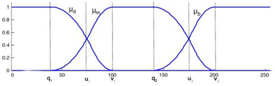
Figure 1. Membership function graph.

The mathematical model of the three membership functions is defined as follows:

$${\mu }_d\left(k\right)=\left\{\begin{array}{cc}1& k\le q_1\\ 1-\frac{{\left(k-q_1\right)}^2}{\left(v_1-q_1\right)\ast \left(u_1-q_1\right)}& q_1\le k\le u_1\\ \frac{{\left(k-v_1\right)}^2}{\left(v_1-q_1\right)\ast \left(v_1-u_1\right)}& u_1\le k\le v_1\\ 0& k\ge v_1\end{array}\right.,$$

(16)

$${\mu }_m\left(k\right)=\left\{\begin{array}{cc}0& k\le q_1\\ \frac{{\left(k-q_1\right)}^2}{\left(v_1-q_1\right)\ast \left(u_1-q_1\right)}& q_1\le k\le u_1\\ 1-\frac{{\left(k-v_1\right)}^2}{\left(v_1-q_1\right)\ast \left(v_1-u_1\right)}& u_1\le k\le v_1\\ 1& v_1\le k\le q_2\end{array}\right.,$$

(17)

$${\mu }_b\left(k\right)=\left\{\begin{array}{cc}0& k\le q_2\\ \frac{{\left(k-q_2\right)}^2}{\left(v_2-q_2\right)\ast \left(u_2-q_2\right)}& q_2\le k\le u_2\\ 1-\frac{{\left(k-v_2\right)}^2}{\left(v_2-q_2\right)\ast \left(v_{21}-u_2\right)}& u_2\le k\le v_2\\ 1& k\ge v_2\end{array}\right.,$$

(18)

the six parameters $q_1$, $u_1$, $v_1$, $q_2$, $u_2$, $v_2$ must fulfill the condition $0\le q_1<u_1<v_1<q_2<u_2<v_2\le 255$. In order to reach the maximum value of entropy, a combination of the membership function’s variables must be found. As a result, the most applicable threshold can be computed as follows:

$$\begin{array}{c}{\mu }_d\left(T_1\right)={\mu }_m\left(T_1\right)=0.5,\\ {\mu }_m\left(T_2\right)={\mu }_b\left(T_2\right)=0.5\end{array}$$

(19)

According to the previous equations, the thresholds $T_1$ and $T_2$ can be computed by Equations (16)–(18) and the result is as following:

$$\begin{array}{cc}\hfill T_1& =\left\{\begin{array}{cc}{q}_1+\sqrt{\left(v_1-q_1\right)\ast \left(u_1-q_1\right)/2}\hfill & \left(q_1+v_1\right)/2⩽u_1⩽v_1\hfill \\ v_1-\sqrt{\left(v_1-q_1\right)\ast \left(v_1-u_1\right)/2}\hfill & q_1⩽u_1⩽\left(q_1+v_1\right)/2\hfill \end{array}\right.,\hfill \\ \hfill T_2& =\left\{\begin{array}{cc}{q}_2+\sqrt{\left(v_2-q_2\right)\ast \left(u_2-q_2\right)/2}\hfill & \left(q_2+v_2\right)/2⩽u_2⩽v_2\hfill \\ v_2-\sqrt{\left(v_1-q_2\right)\ast \left(v_2-u_2\right)/2}\hfill & q_2⩽u_2⩽\left(q_2+v_2\right)/2\hfill \end{array}\right..\hfill \end{array}$$

(20)

2.3.2. Otsu Method

The Otsu technique [51] is one of the most commonly utilized segmentation methods for finding optimal threshold values by maximizing the class variance. The intensity levels L for each color image are within the range $0,1,2,\dots L-1$. The probability distribution of the intensity value is computed as follows:

$$P{h}_j=\frac{N_j}{nk},P{h}_j\ge 0,\sum _{j=1}^{L}P{h}_j=1,$$

(21)

where $nk$ denotes the number of pixels in the image and j is an intensity level in the range $(0\le j\le L-1)$. The number of gray level i in the image represented by the histogram is $N_i$, and the probability distribution of the intensity levels is $P{h}_j$. For bi-level segmentation, the classes are computed as follows:

$$C_a=\frac{P{h}_1}{{\omega }_1\left(th\right)},\dots ,\frac{P{h}_{th}}{{\omega }_1\left(th\right)}\mathrm{and}{C}_b=\frac{P{h}_{th+1}^c}{{\omega }_2\left(th\right)},\dots ,\frac{P{h}_L}{{\omega }_2\left(th\right)}.$$

(22)

where ${\omega }_1\left(th\right)$ and ${\omega }_2\left(th\right)$ are the cumulative probability distributions for $C_a$ and $C_b$, respectively. ${\omega }_1\left(th\right)$ and ${\omega }_2\left(th\right)$ can be computed by the following:

$${\omega }_1\left(th\right)=\sum _{j=1}^{th}P{h}_j\mathrm{and}{\omega }_2\left(th\right)=\sum _{th+1}^{L}P{h}_j.$$

(23)

The mean levels ${\mu }_1$ and ${\mu }_2$ must be computed that define the classes using Equation (24). Equation (25) is used for computing the Otsu-based between-class ${\sigma }_A^2$.

$${\mu }_1=\sum _{j=1}^{th}{\displaystyle \frac{jP{h}_j}{{\omega }_1\left(th\right)}}\mathrm{and}{\mu }_2=\sum _{j=th+1}^L{\displaystyle \frac{jP{h}_j}{{\omega }_2\left(th\right)}},$$

(24)

$${\sigma }_A^2={\sigma }_a+{\sigma }_b.$$

(25)

Additionally, ${\sigma }_a$ and ${\sigma }_b$ are the variance of $C_a$ and $C_b$ and are calculated as follows:

$${\sigma }_a={\omega }_1{({\mu }_1+{\mu }_T)}^2\mathrm{and}{\sigma }_b={\omega }_2{({\mu }_2+{\mu }_T)}^2,$$

(26)

where ${\mu }_T={\omega }_1{\mu }_1+{\omega }_2{\mu }_2$ and ${\omega }_1+{\omega }_2=1$ based on the values ${\sigma }_a$ and ${\sigma }_b$, the objective function is defined by Equation (27). As a result, the optimization problem is decreased to determine the intensity level that maximizes Equation (27):

$$F_{otsu}\left(th\right)=max\left({\sigma }_A^2\left(th\right)\right)\mathrm{where}0\le th\le L-1,$$

(27)

where the Otsu method variance for a given $th$ value is ${\sigma }_A^2\left(th\right)$. EBO methods are utilized for determining the intensity level $th$ to maximize the objective function according to Equation (27). The objective or fitness function $F_{otsu}\left(th\right)$ can be modulated for multiple thresholds as:

$$F_{otsu}\left(TH\right)=\mathit{Max}\left({\sigma }_A^2\left(th\right)\right)\mathrm{where}0\le th\le L-1\mathrm{and}j=[1,2,3,\dots ,n],$$

(28)

where $TH=[t{h}_1,t{h}_2,\dots ,t{h}_n-1]$ illustrates a vector including MTH, and the variance is calculated by Equation (29).

$$N{\sigma }_A^2=\sum _{j=1}^n{\sigma }_j=\sum _{j=1}^n{\omega }_2{({\mu }_2-{\mu }_T)}^2.$$

(29)

${\mu }_j$ is the mean of a class, ${\omega }_j$ is the occurrence probability, and j represents a specific class.

3. The Proposed mSAR

In this section, a new technique that improves SAR is explained in detail and called mSAR. The SAR algorithm is improved based on OBL as a local research strategy to reinforce the convergence of the algorithm by enhancing the variety of its solutions and avoiding the drawbacks of the random population. As a result, mSAR utilizes OBL in the initialization phase to improve the search process as follows:

$$O_j=L{B}_i+U{B}_i-X_j,j\in 1,2,\dots ,n,$$

(30)

where $O_j$ is a vector-maintaining solution obtained by using OBL. $L{B}_i$ and $U{B}_i$ are the lower and upper bounds of the $i^{th}$ component of a vector X. Finally, the phases below are given further detail on the phases of the proposed image thresholding model.

3.1. Initialization Phase in mSAR

In the first phase, the proposed model begins by reading the image from the benchmark dataset, calculating the histogram of the selected image, and calculating the probability distribution of the selected images by Equation (13). In the next step, the algorithm initializes the mSAR parameters, such as problem dimensions D, population size N, boundaries of the search space ($L{B}_i$, $U{B}_i$), and the maximum iteration number T. The SAR, like many other optimization algorithms, begins by randomly initializing the first population $x^0$ and then storing the results. Following that, the OBL concept is used to compute the $O_j$ vector maintaining solution using Equation (30).

3.2. Optimization Phase

During this phase, we estimate the fitness values of the $X_j$ and $O_j$ populations to determine the optimal algorithmic threshold values. For updating the search agents’ locations, use the fitness value of the best threshold of the fuzzy entropy [52] or the Otsu [51] methods as the fitness function, and then compare the fitness values of $O_j$ and $X_j$ and store the optimal solution with the highest fitness. The optimization algorithm processes are split into two stages: the social and individual stages, as studied in the subsection on SAR. Following the implementation of the two phases of the optimization algorithm, each search agent updates its location repeatedly based on the best fitness values of $O_j$ and $X_j$, using the fuzzy entropy Equation (19) or the Otsu Equation (28), as described in Algorithm 1. The flowchart of the proposed mSAR algorithm is represented in Figure 2.

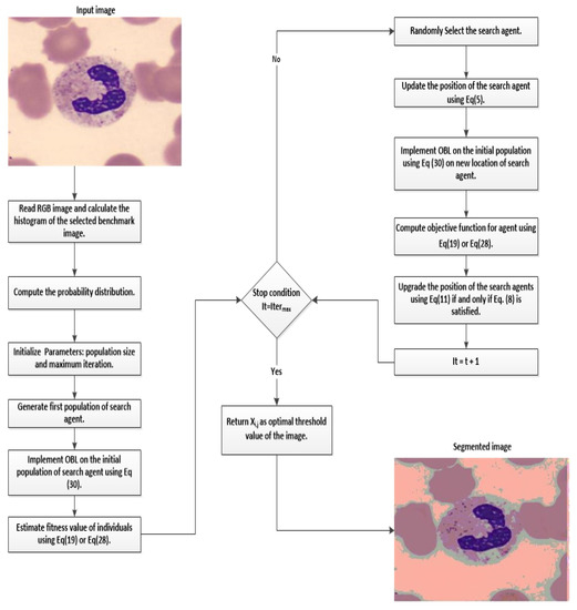
Figure 2. The flowchart of mSAR algorithm.

3.3. Final Phase of mSAR

After executing the optimization phase, fitness upgrade, memory storing, and search agents’ location upgrade using Equation (30), the proposed algorithm selects the optimal threshold values to generate the segmented image. The pseudo-code of the proposed algorithm is displayed in Algorithm 1.

Algorithm 1 The proposed mSAR algorithm

Input: Set parameters values ($N=50$, $P=0.5$, $T_{\mathit{max}}=350$, $t=30$, $SE=0.05$);

Output: Return the optimal solution with the optimal threshold values onto the image.

Generate the first population $X_j^0$ randomly with dimensions D.

Utilize Equation (30) to apply OBL on the first population $X_j^0$ and save outcomes in $O_j$.

while $(t\le Ite{r}_{\mathit{max}})$ do

for $j\le N$ do

Estimate $X_j$ utilizing fuzzy entropy Equation (19) or Otsu Equation (28) and save outcomes in $fi{t}_j$.

Estimate $O_j$ utilizing fuzzy entropy Equation (19) or Otsu Equation (28) and save outcomes in $Fit{O}_j$.

if $Fi{t}_j<Fit{O}_j$ then

$X_j=O_j;$

end if

end for

Complete the memory saving.

if $t<\frac{Ite{r}_{\mathit{max}}}{3}$ then

Upgrade nominee solutions by Equation (9).

else if $\frac{Ite{r}_{\mathit{max}}}{3}<t<2\times \frac{Ite{r}_{\mathit{max}}}{3}$ then

Upgrade search agents’ location by Equation (11).

else if $t>2\times \frac{Ite{r}_{\mathit{max}}}{3}$ then

Upgrade nominee solutions by Equation (30).

end if

The optimal solution found so far will update.

for each candidate solution do

Estimate $X_j$ after upgrade by fuzzy entropy Equation (19) or Otsu Equation (28) and save outcomes in $fi{t}_j$.

Estimate $O_j$ after upgrade by fuzzy entropy Equation (19) or Otsu Equation (28) and save outcomes in $Fit{O}_j$.

if $Fi{t}_j<Fit{O}_j$ then

Set $X_j=O_j;$

end if

end for

Execute memory storing and fitness updates.

Define the optimal value of search agents’ location.

Save the outcomes.

end while

Return the optimal solution with the optimal threshold values onto the image.

3.4. Computational Complexity of mSAR

This subsection illustrates the computational complexity of the proposed mSAR. Firstly, the complexity of the initialization process can be described as $\mathcal{O}(2\times N\times D)$, where N and D indicate the number of search agents and the dimension of the problem, respectively. During the initialization phase of the mSAR algorithm, sorting the search agent takes $O\left(2N\log \right(2N\left)\right)$ times. In the worst cases, the complexity of the social and individual phases is $\mathcal{O}(N\times D)$. However, the complexity of the abandoning clue and restart processes in the worst cases are $\mathcal{O}(N\times D)$. Furthermore, $O\left(T\right)$ time complexity is required for mSAR to execute T of its main operations (initialization phase, social phase, abandoning clue, individual phase, restart strategy, and OBL). As a result, the mSAR computes the fitness of each agent with complexity as follows:

$$\begin{array}{c}O\left(mSAR\right)=O(2\times N\times D)+O\left(2N\log \left(2N\right)\right)+t_{max}\times (O(N\times D)\\ +O(N\times D)+O(N\times D)+O(N\times D))\end{array}$$

(31)

Overall, the total computational complexity of the proposed mSAR can be represented by $\mathcal{O}(T\times t_{max}\times N\times D)$.

4. Performance Evaluation of mSAR on CEC’20 Test Suit

4.1. Parameter Settings of CEC’2020

In this subsection, the evaluation of the proposed mSAR algorithm is introduced. Therefore, the proposed mSAR algorithm used the IEEE Congress on Evolutionary Computation (CEC) [53] as a test problem for estimating the algorithms’ performance. The performance of mSAR is estimated over the CEC’2020 benchmark functions. Firstly, this benchmark function includes 10 test problems and can be classified into four types. This benchmark function includes unimodal, multimodal, hybrid, and composition functions. The mathematical formulation and parameter-setting of the CEC’2020 benchmark test are shown in Table 1; ’Fi*’ indicates the optimal global value. A two-dimensional visualization of the CEC’2020 functions is shown in Figure 3 to explain the differences and the nature of each problem.

Table 1. CEC’2020 benchmark functions.

No.	Function Description	Fi*
Unimodal function
F1	Shifted and Rotated Bent Cigar Function	100
Multimodal shifted and rotated functions
F2	Shifted and Rotated Schwefel’s Function	1100
F3	Shifted and Rotated Lunacek bi-Rastrigin Function	700
F4	Expanded Rosenbrock’s plus Griewangk’s Function	1900
Hybrid functions
F5	Hybrid Function 1 (N = 3)	1700
F6	Hybrid Function 2 (N = 4)	1600
F7	Hybrid Function 3 (N = 5)	2100
Composition functions
F8	Composition Function 1 (N = 3)	2200
F9	Composition Function 2 (N = 4)	2400
F10	Composition Function 3 (N = 5)	2500

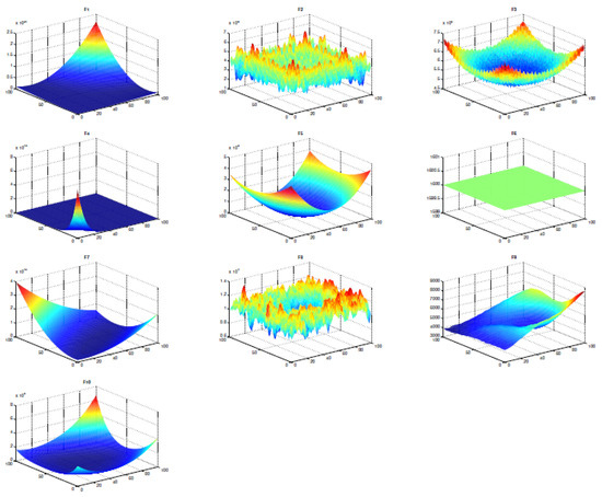
Figure 3. CEC’2020 benchmark functions in two-dimensional view.

4.2. Statistical Results Analysis

The performance of the proposed mSAR is estimated by utilizing the CEC’2020 benchmark test, which contains qualitative and quantitative metrics. The mean and standard deviation (STD) of optimal solutions obtained by the proposed algorithm and all other algorithms compared are quantitative metrics. Furthermore, the average fitness history, search history, and convergence curve are qualitative metrics. We utilized these qualitative metrics for estimating the performance of the proposed mSAR on the CEC’2020 benchmark test against seven well-known metaheuristic algorithms, namely LFD, HHO, SCA, EO, GSA, AOA, and the original SAR. The STD and mean of the optimum value produced from the proposed mSAR algorithm against other competing algorithms are illustrated in Table 2, and the optimum value of the mean and STD are minimum values in outcomes. According to the STD and mean results in Table 2, the proposed mSAR algorithm outperforms other competing algorithms on the CEC’2020 benchmark functions.

Table 2. STD and mean of the optimum value obtained from the proposed mSAR algorithm against other competing algorithms on the CEC’2020 benchmark functions with $D=20$.

Functions	LFD		HHO		SCA		EO		GSA		AOA		SAR		mSAR
	Mean	Std	Mean	Std	Mean	Std	Mean	Std	Mean	Std	Mean	Std	Mean	Std	Mean	Std
F1	2.583E+10	3.262E+06	4.733E+06	1.350E+05	8.256E+09	3.102E+04	2.307E+03	1.304E+09	4.593E+09	4.652E+03	3.398E+09	3.130E+03	1.427E+06	3.560E+01	3.942E+08	1.418E+07
F2	4.647E+03	3.201E+02	3.032E+03	2.970E+04	4.892E+03	4.028E+03	4.220E+03	6.356E+03	4.685E+04	6.301E+01	4.084E+03	4.264E+02	3.236E+03	2.003E+02	2.496E+03	2.537E+03
F3	1.056E+03	2.040E+01	9.340E+02	6.623E+01	9.376E+02	3.601E+01	7.478E+02	2.630E+01	8.686E+02	2.655E+03	8.779E+02	6.120E+03	7.721E+02	3.784E+05	1.077E+02	6.835E+02
F4	1.636E+05	8.611E+00	1.919E+03	1.301E+03	3.277E+03	5.103E+00	1.903E+03	9.319E+03	6.343E+04	2.368E+06	2.472E+03	1.442E+00	1.906E+03	2.230E+01	6.471E+03	5.651E+05
F5	4.908E+06	3.120E+04	6.073E+04	6.310E+04	1.152E+06	7.214E+04	1.454E+05	6.531E+01	8.328E+07	3.791E+02	1.525E+06	1.681E+02	5.776E+05	6.552E+03	1.447E+04	7.658E+03
F6	1.667E+03	2.119E+05	1.857E+03	2.014E+02	2.049E+03	1.620E+01	1.624E+03	9.300E+01	1.624E+03	6.240E+02	2.371E+03	0.000E+00	2.049E+03	3.567E+03	1.883E+02	4.681E+01
F7	1.891E+06	9.101E+07	3.251E+05	7.302E+01	2.718E+05	2.531E+05	9.194E+04	3.613E+04	2.144E+06	0.000E+00	1.745E+05	6.067E+03	3.955E+03	0.000E+00	1.056E+03	3.597E+02
F8	5.111E+03	4.715E+03	2.305E+03	5.200E+00	3.165E+03	1.435E+03	2.597E+03	7.020E+03	4.968E+04	6.234E+01	5.021E+03	2.641E+05	2.311E+03	6.302E+06	6.491E+03	0.000E+00
F9	3.022E+03	2.605E+06	3.258E+03	4.106E+04	2.975E+03	6.165E+02	2.827E+03	5.460E+02	3.533E+03	1.563E+06	2.985E+03	6.340E+04	2.910E+03	3.409E+02	1.004E+03	3.564E+03
F10	4.505E+03	3.106E+03	3.005E+03	5.780E+03	3.220E+03	3.031E+03	2.931E+04	3.631E+00	3.310E+05	2.061E+02	3.162E+03	5.987E+02	2.913E+03	1.613E+05	2.139E+03	5.651E+04
Friedman mean rank	6.60		3.80		5.55		2.95		6.75		5.00		2.95		2.40
Rank	7		4		6		2		8		5		3		1

4.3. Boxplot Analysis of mSAR Algorithm

Boxplot analysis is utilized to represent the data distribution characteristics. The boxplot analysis indicates the quality of the optimizers’ solutions and is used for reporting data with a homogeneous variance and a normal distribution. Figure 4 illustrates the outcomes of the boxplot of the proposed mSAR algorithm compared with other competitive algorithms. The boxplot is an excellent plot for showing data distributions in quartiles. The maximum and minimum are the highest and lowest data points acquired by the algorithm, which are the whiskers’ edges. These quartiles are the lower and upper quartiles, which are determined by the ends of the rectangles, and a narrow boxplot indicates the highest agreement among data. The outcomes of the boxplot of the proposed mSAR algorithm with other competitive algorithms and the outcomes of the ten functions boxplot for D = 20 are illustrated in Figure 4. Indeed, the proposed mSAR algorithm outperforms other competing algorithms on the majority of the benchmark functions, but its performance on $F3$ and $F7$ is limited.

Figure 4. The outcomes of the boxplot of the proposed mSAR algorithm with other competitive algorithms over CEC’2020 functions with $D=20$.

4.4. Curves of Convergence of mSAR Algorithm

This subsection describes the convergence curves of the proposed SAR algorithm and other competing algorithms. The convergence curves of SCA, HHO, AOA, EO, LFD, GSA, SAR, and mSAR for the CEC’2020 functions are shown in Figure 5. Moreover, the mSAR algorithm reached a stable point for most functions and acquired optimal solutions for an algorithm. Therefore, most problems that need fast computation, such as online optimization problems, can be solved by the mSAR algorithm. The mSAR algorithm displayed stable behavior, and due to space limitations, its solutions converged quickly in most of the problems in which it was evaluated.

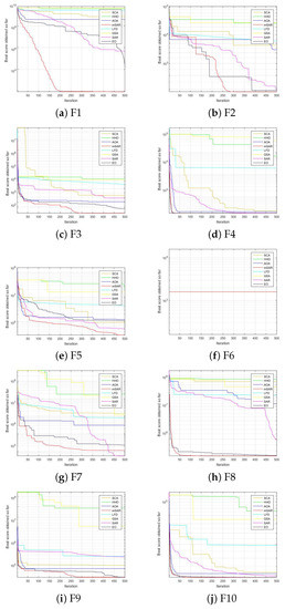
Figure 5. The convergence curves of the proposed mSAR algorithm with other competitive algorithms over CEC’2020 functions with $D=20$.

4.5. Qualitative Metrics

Even though previous outcome studies assured the proposed mSAR algorithms’ superior performance, more experiments and analyses would help us draw more definitive conclusions regarding the algorithms’ performance in solving real problems. The qualitative analysis of the mSAR algorithm is illustrated in Figure 6. The first and second columns in the figure describe the CEC’2020 benchmark functions in two-dimensional space and show the search history of the agent. The average fitness history over 350 iterations is shown in the third column, which explains the agents’ overall behavior and their contribution to locating the optimum solution. Most of the history curves gradually decrease according to average fitness history, indicating that the population improves with each iteration. The optimization history and convergence curve are shown in the fourth column. The optimization history is reduced according to Figure 6. This means that the solution is optimized during iterations until the best solution is found.

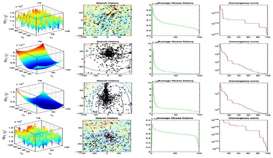
Figure 6. Qualitative metrics on F2, F5, F6, and F8: functions in 2D view, search history, average fitness history, and convergence curve.

5. Application of mSAR: Blood Cells Images Segmentation

The experimental environment of the proposed mSAR algorithm is illustrated in this section. The test images used for the experiments are presented first, followed by the empirical setup. Then, we analyzed the outcomes acquired by mSAR in terms of PSNR, SSIM, FSIM, and fitness.

5.1. Benchmark Images

To examine the performance of the proposed mSAR algorithm and determine the best threshold values, eight images of the benchmark were used. These images were taken in the core laboratory at the Hospital Clinic of Barcelona during the diagnosis of malaria infection [54]. The images in the dataset are in the format JPG (RGB, 2400 × 1800 pixels). These images have different features based on their histograms, as observed in Figure 7. The purpose of selecting these images is to test the performance and quality of the segmented images.

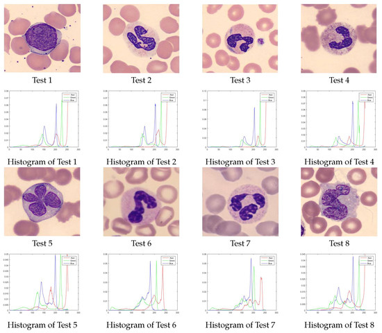
Figure 7. Set of test images and relative histograms.

5.2. Experimental Setup

This subsection compares the proposed mSAR algorithm to seven metaheuristic algorithms: LFD [8], HHO [37], SCA [55], EO [56], GSA [26], AOA [57], and the original SAR [38]. All experiments were implemented in Matlab 2015 and executed on an Intel Core I5 with 6 GB of RAM running in a Windows 8.1 64-bit environment. To achieve a fair comparison, all competitor algorithms executed 30 runs per test image, the maximum number of iterations was set to 350, and the population was 50. Each algorithm’s parameter settings were defined using standard criteria and information from previous literature (default values). All experiments were executed on images using various thresholds: are $t{h}_2,t{h}_5,t{h}_7,$ and $t{h}_{10}$ according to related literature [58]. Table 3 presents the parameter settings of the mSAR algorithm and its value.

Table 3. The parameter settings of the mSAR algorithm and its value.

Parameter	Value
Maximum iterations $\left(T_{\mathit{max}}\right)$	350
Number of independent runs $\left(t\right)$	30
Population size $\left(N\right)$	50
Dimension of problem $\left(Dim\right)$	20
Mutation ratio $\left(P\right)$	0.5
Social effect parameter $\left(SE\right)$	0.05

5.3. Performance Metrics

Five metrics were used for evaluating the quality of the image and comparing the edges of the segmented images: Wilcoxon rank test, standard deviation (STD), peak signal-to-noise ratio (PSNR) [59], feature similarity (FSIM) [60], and structural similarity (SSIM) [61]. The algorithm becomes more stable when the value of STD is decreased by [62]. The STD can be defined as follows:

$$STD=\sqrt{\sum _{j=1}^n\frac{{\sigma }_j-\mu }{n}},$$

(32)

where n is the total number of pixels in the image, $\mu$ is the mean of pixels, and ${\sigma }_j$ is the value of jth in the image.

5.3.1. Peak Signal-To-Noise Ratio (PSNR)

PSNR [59,60] is a metric utilized for estimating the performance of the segmented image and computing the difference between the original image and its segmented image, and defined as follows:

$$\begin{array}{cc}\hfill PSNR& =20{\log }_{10}\left({\displaystyle \frac{255}{RMSE}}\right),\hfill \\ \hfill RMSE& =\sqrt{({\displaystyle \frac{{\sum }_{j=1}^{n_r}{\sum }_{i=1}^{n_c}\left({(I(j,i)-Seg(j,i))}^2\right)}{n_r\times n_c}})}.\hfill \end{array}$$

(33)

In Equation (33), I is the original image, and $Seg$ is the segmented image of size $n_r\times n_c$. The root-mean-squared error is $RMSE$.

5.3.2. Feature Similarity Index (FSIM)

FSIM [61] is another measure used to map the features and measure the similarities based on the internal features of the image. FSIM is computed by the following:

$$FSIM=\frac{{\sum }_{uϵ\mathrm{\Omega }}{S}_L\left(u\right)P{C}_n\left(u\right)}{{\sum }_{uϵ\mathrm{\Omega }}P{C}_n\left(u\right)},$$

(34)

where the entire domain of the image is $\mathrm{\Omega }$, and the value of $P{C}_n\left(u\right)$ is described as follows:

$$PC=\frac{E\left(\omega \right)}{\left(ϵ+{\sum }_n{A}_n\left(\omega \right)\right)},$$

(35)

where the magnitude of the vector in $\omega$ on n is $E\left(\omega \right)$, and the amplitude’s local on scale n is $A_n\left(\omega \right)$. $ϵ$ is the small positive value and $P{C}_n\left(u\right)=max\left(P{C}_1\left(u\right),PC2\left(u\right)\right)$.

5.3.3. Structural Similarity Index (SSIM)

The value of SSIM is higher when the original image will be better segmented because the structures in the two images match. SSIM is defined in Equation (36).

$$SSIM(I,Seg)={\displaystyle \frac{(2{\mu }_1{\mu }_{Seg}+c_a)(2{\sigma }_{1,Seg}+c_b)}{({\mu }_I^2+{\mu }_{Seg}^2+c_a)({\sigma }_I^1+{\sigma }_{Seg}^2+c_b)}},$$

(36)

where the mean value of segmented image $\left(Seg\right)$ and the original image I are ${\mu }_{Seg}$ and ${\mu }_I$, respectively. The standard deviation values of segmented image $\left(Seg\right)$ and the original image I are ${\sigma }_{Seg}$ and ${\sigma }_I$, respectively. $c_a$ and $c_b$ are two constant numbers, and the covariance of I and $Seg$ is ${\sigma }_{I,Seg}$.

5.3.4. Wilcoxon Rank-Sum Test

The Wilcoxon rank-sum test is a non-parametric test that determines if two independent samples come from the same population distribution [63]; it is also utilized to compare the results obtained by algorithms. The test is constructed with two hypotheses in mind: the null hypothesis and the alternative hypothesis. According to the values of $\left(P\right)$ and $\left(H\right)$, the value of the null hypothesis is true when (p > 0.05) or $(H=0)$, but the value of the alternative hypothesis is true when (p < 0.05) or $(H=1)$.

5.3.5. Friedman Mean Rank Test

The Friedman test is also a non-parametric statistical test utilized to find differences in treatments across three or more matched groups and evaluate the performance of the competitive algorithms. This statistical test is utilized for one-way repeated measures analysis of variance by the value of ranks and was generated by Milton Friedman [64]. The values of the mean ranked are computed by Friedman’s statistics [64]. Friedman’s statistics compare the critical values obtained from competitors’ algorithms to see whether the null hypothesis is rejected or not.

5.4. Results Analysis of the Proposed Algorithm Based on Fuzzy Entropy

This subsection discusses and analyzes the outcomes of the proposed algorithm mSAR using different numbers of thresholds [$nTh=2,5,7,10$]. The fuzzy entropy method is used in this section as an objective function to obtain optimal thresholds.

Figure A1 in Appendix A illustrates the resulting images of the mSAR algorithm with various numbers of thresholds for all the test images utilized in the experiments. Figure 8 illustrates the resulting images of the mSAR with a different number of thresholds over test image 2 and presents a graphical analysis of the thresholds of the segmented images. The optimal thresholding values obtained by the mSAR algorithm and the original SAR algorithm using the fuzzy entropy method are shown in Table A1 in Appendix A. The mean and STD outcomes of the fitness, PSNR, SSIM, and FSIM are illustrated in Table 4, Table 5, Table 6 and Table 7, respectively. When the mean value of an algorithm is high, the algorithm is efficient and accurate. Hwoever, when the value of the STD of an algorithm is low, the algorithm is more stable.

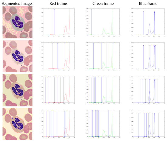
Figure 8. Threshold outcomes of each layer of a color image using the mSAR algorithm with the fuzzy entropy method.

Table 4. mSAR fuzzy entropy in terms of fitness values over all competed algorithms.

		LFD		HHO		SCA		EO		GSA		AOA		SAR		mSAR
Test Image	nTh	Mean	Std	Mean	Std	Mean	Std	Mean	Std	Mean	Std	Mean	Std	Mean	Std	Mean	Std
Test 1	2	18.1046	2.8080E-16	18.0759	2.8440E-16	18.1062	2.7720E-16	18.0876	2.9991E-04	18.0261	2.7360E-16	18.0082	1.9760E-02	18.2110	2.5560E-16	18.1255	2.4120E-16
	5	22.6431	2.8080E-16	22.6264	2.8440E-16	22.6153	3.9963E-03	22.5722	2.1917E-03	22.5199	1.3756E-03	22.6169	2.7360E-16	22.7893	2.5560E-16	22.6808	2.4120E-16
	7	27.3154	1.9500E-04	27.3259	8.5320E-16	27.3560	1.1935E-03	27.0981	4.7140E-03	27.1008	1.1400E-04	27.3199	1.7480E-04	27.3184	7.6680E-16	27.3903	7.2360E-16
	10	31.3638	1.9500E-04	31.4052	1.5642E-03	31.4301	2.1637E-03	31.0209	7.9976E-03	31.1137	5.0236E-03	31.3801	3.5796E-03	31.4205	2.5560E-16	31.5391	2.4120E-16
Test 2	2	18.3414	2.8080E-16	18.3139	2.8440E-16	18.3425	2.7720E-16	18.3344	1.3073E-04	18.2793	2.6752E-15	18.3072	2.7360E-16	18.3491	2.5560E-16	18.3964	2.4120E-16
	5	22.9591	2.7066E-15	23.7630	9.4010E-03	22.8547	9.2400E-03	23.7630	2.8684E-03	22.8249	6.3916E-03	22.7600	7.3188E-03	23.1217	2.5560E-16	23.0566	2.4120E-16
	7	27.3599	1.2246E-05	27.3536	1.2087E-05	27.3652	8.5470E-03	27.4435	5.2061E-03	27.1778	4.6436E-05	27.1115	2.3940E-02	27.4506	1.0224E-15	27.4735	9.6480E-16
	10	31.3065	4.0560E-04	31.3372	8.6900E-04	31.3677	8.1620E-04	31.4664	1.0151E-02	31.1128	1.0412E-03	31.1385	2.5916E-02	31.3560	1.2780E-15	31.4664	1.2060E-15
Test 3	2	18.1695	2.8080E-16	18.1460	2.8440E-16	18.1701	2.7720E-16	18.1662	6.4135E-05	18.1142	8.1320E-15	18.1351	2.7360E-16	18.1700	2.5560E-16	18.2409	2.4120E-16
	5	22.7428	3.3306E-03	22.7042	1.8170E-03	22.8149	1.0318E-05	22.6968	4.4602E-04	22.6584	3.1616E-03	22.6843	1.3680E-15	22.7794	2.9465E-03	22.8716	2.7805E-03
	7	27.2930	2.8860E-04	27.1417	1.5642E-02	27.3592	3.6190E-04	26.9526	7.0979E-03	26.9972	1.4668E-02	26.9902	1.1172E-02	27.3330	5.1191E-16	27.4420	4.8307E-16
	10	31.4630	8.2680E-04	31.4970	1.5326E-02	31.5696	7.0070E-04	30.8451	1.3996E-02	31.1545	2.0900E-02	31.1630	2.5536E-02	31.5604	7.6680E-16	31.6866	7.2360E-16
Test 4	2	18.4294	1.1232E-15	18.4057	1.1376E-15	18.4300	2.4178E-07	18.4208	1.9994E-04	18.3649	1.0944E-15	18.3944	1.0944E-15	18.4295	1.0224E-15	18.4020	1.0656E-15
	5	23.2453	2.6208E-06	23.2518	8.5320E-16	23.2511	9.2400E-05	23.1999	9.3818E-04	23.1441	8.2080E-16	23.2088	8.2080E-16	23.2518	7.6680E-16	23.2427	7.9920E-16
	7	27.5700	2.7300E-05	27.5607	3.8789E-05	27.5948	3.3572E-05	27.4411	2.6223E-03	27.4436	1.1400E-04	27.5443	1.4136E-05	27.5907	2.5560E-16	27.5619	2.6640E-16
	10	31.6329	2.9718E-03	31.6810	4.8980E-03	31.7427	1.1319E-03	31.7427	5.2907E-03	31.4583	6.2548E-03	31.5898	5.7608E-03	31.7314	2.5560E-16	31.0452	2.6640E-16
Test 5	2	18.1587	2.8080E-16	18.1330	2.8440E-16	18.1594	2.7720E-16	18.1546	6.8133E-05	18.0990	2.1584E-15	18.1242	2.7360E-16	18.1766	2.5560E-16	18.3358	2.6640E-16
	5	23.0376	5.7408E-15	23.0165	8.5320E-16	23.0426	2.1637E-03	22.9820	1.2919E-03	22.9274	9.8800E-15	23.0065	8.2080E-16	23.0698	7.6680E-16	23.2735	7.9920E-16
	7	27.6085	1.6380E-04	27.4755	2.1251E-02	27.6783	1.2782E-02	27.0664	1.2996E-02	27.3479	1.5580E-02	27.3909	2.0520E-02	27.7290	1.2780E-15	27.9806	1.3140E-15
	10	31.6238	2.2074E-03	31.7292	2.0935E-02	31.8116	1.0626E-02	30.7854	1.7918E-02	31.3514	2.1660E-02	31.4811	2.3712E-02	31.8731	7.6680E-06	31.8507	2.6280E-16
Test 6	2	18.7103	5.6238E-16	18.6849	5.6959E-16	18.7108	5.5517E-16	18.7053	1.1535E-04	18.6505	5.4796E-16	18.6745	5.4796E-16	18.7088	5.1191E-16	18.7111	5.2633E-16
	5	23.2793	1.3260E-04	23.2549	1.0428E-05	23.2864	2.2330E-04	23.2476	9.2280E-04	23.1915	1.9760E-04	23.2411	3.6176E-06	23.2909	2.3430E-04	23.2886	2.6280E-04
	7	27.7771	4.9218E-05	27.7951	5.6485E-03	27.8501	6.8838E-05	27.5574	5.4215E-03	27.6000	5.4872E-03	27.6920	9.5760E-03	27.8342	1.2780E-15	27.8501	1.3140E-15
	10	31.8757	4.6020E-04	31.9350	4.1870E-04	31.9670	1.1858E-03	31.9953	8.4590E-03	31.6525	1.1096E-03	31.8810	2.4472E-03	31.9853	0.0000E+00	31.9701	0.0000E+00
Test 7	2	18.4319	2.8080E-16	18.4087	1.8802E-05	18.4334	1.1242E-05	18.4237	2.6915E-04	18.3675	1.6188E-05	18.3981	8.5880E-06	18.4509	2.5560E-16	18.5410	2.7360E-16
	5	23.0903	8.4240E-16	23.0759	6.1462E-05	23.1040	1.6940E-04	23.0421	1.1381E-03	22.9856	1.2160E-04	23.0633	8.2080E-16	23.1266	7.6680E-16	23.2402	8.2080E-16
	7	27.3927	7.8000E-05	27.3945	6.0040E-04	27.4277	6.0830E-04	27.2754	3.2375E-03	27.2679	4.8640E-04	27.3820	3.9520E-04	27.4576	1.7892E-15	27.5938	1.9152E-15
	10	31.3324	4.3680E-04	31.3642	5.6880E-04	31.3989	1.2551E-03	31.0497	6.7903E-03	31.1869	9.1960E-04	31.3404	1.1020E-03	31.4269	2.0448E-15	31.5843	1.9872E-15
Test 8	2	18.3020	1.1232E-15	18.2744	1.1376E-15	18.3069	7.9310E-06	18.1867	9.9970E-04	18.1901	1.0944E-15	18.0382	3.2604E-02	18.3211	1.0224E-15	18.3211	9.9360E-16
	5	23.0376	5.7408E-05	23.0578	8.5320E-16	22.9703	1.3552E-02	22.7504	5.9444E-03	23.1041	2.3560E-04	23.0521	8.2080E-16	23.1041	7.6680E-16	23.0448	7.4520E-16
	7	27.1252	1.4820E-04	27.1816	2.6781E-05	27.1951	3.8808E-03	26.7231	9.2280E-03	26.8257	2.2040E-04	27.1838	1.3680E-04	27.2266	7.6680E-16	27.3973	7.4520E-16
	10	30.8359	2.0436E-03	30.9707	1.5484E-03	31.0086	2.7258E-03	29.9156	5.1062E-02	30.5448	1.8316E-03	30.8748	1.5732E-02	31.0187	5.1191E-16	31.2114	4.9749E-16

Table 5. mSAR fuzzy entropy in terms of PSNR values over all competed algorithms.

		LFD		HHO		SCA		EO		GSA		AOA		SAR		mSAR
Test Image	nTh	Mean	Std	Mean	Std	Mean	Std	Mean	Std	Mean	Std	Mean	Std	Mean	Std	Mean	Std
Test 1	2	14.0348	5.5380E-14	14.0484	4.6150E-14	14.1710	6.4610E-13	14.02757	5.3520E-02	13.9516	4.6150E-13	14.0100	5.5380E-13	14.0820	9.7308E-12	14.1710	4.4304E-13
	5	14.8938	2.2700E-04	14.9083	8.3000E-04	16.7024	3.9900E-03	15.04624	3.3600E-01	12.4478	2.3050E-13	14.8360	0.0000E+00	14.9227	5.8428E-12	15.0384	2.2128E-13
	7	20.7545	1.6860E-03	20.7777	2.0200E-03	20.9695	2.4430E-02	20.22302	1.1340E+01	12.9449	1.1550E-12	20.6739	5.5800E-03	20.7979	0.0000E+00	20.9591	1.1088E-12
	10	21.2726	4.2840E-03	21.3499	2.3050E-03	21.6258	6.8600E-03	20.89767	8.6400E+00	13.7842	6.7500E-01	21.2618	7.3800E-03	21.6922	1.5552E-11	21.4874	1.1088E-12
Test 2	2	15.0771	4.1520E-14	15.0918	3.4600E-14	15.0235	4.8440E-13	15.07096	4.9500E-02	14.0941	3.4600E-13	15.0186	4.1520E-13	15.1064	5.8428E-12	15.2771	3.3216E-13
	5	16.7056	5.5380E-14	17.2239	1.2500E-03	17.5063	6.4610E-13	16.70248	4.9200E-01	12.1618	4.6150E-13	17.5733	2.7660E-13	16.7380	7.7868E-12	16.7056	4.4304E-13
	7	19.8656	1.1940E-03	19.8849	2.0700E-03	20.0460	1.0500E+01	19.42992	1.7580E+01	15.7123	2.3050E-13	19.7146	8.2800E-03	19.9042	3.8880E-12	20.0656	2.2128E-13
	10	21.5301	3.6360E-01	21.5098	3.4100E-02	21.6965	5.1450E+00	20.87707	1.2300E+01	17.5084	2.8900E-01	21.1859	4.6140E-01	21.5595	1.9440E-11	21.7431	0.0000E+00
Test 3	2	16.4975	0.0000E+00	16.5135	0.0000E+00	16.6577	0.0000E+00	16.7577	7.2000E-02	14.1762	0.0000E+00	16.4334	0.0000E+00	16.5295	3.8880E-12	16.7577	0.0000E+00
	5	18.1259	2.4000E-04	19.1838	2.6550E-03	16.6577	4.8440E-13	19.1889	1.7340E+01	15.9442	3.4600E-13	19.2519	1.7400E-03	17.1444	1.2639E+03	17.2442	3.3216E-13
	7	19.1467	9.6000E-04	20.1591	3.1100E-03	19.4750	1.2040E-02	18.85518	1.4340E+01	15.3015	1.4450E-04	20.6370	5.4600E-03	19.3269	0.0000E+00	19.4395	0.0000E+00
	10	21.0007	3.2400E-03	21.2561	2.6650E-02	21.2930	3.0310E+00	19.6112	1.2120E+01	15.4606	1.1500E-03	21.8600	3.6000E-02	21.0666	7.7868E-12	21.8624	3.3216E-13
Test 4	2	15.6581	8.2800E-14	15.6733	6.9000E-14	15.8101	9.6600E-13	15.63334	2.5200E-02	15.6291	6.9000E-13	15.5973	5.5380E-13	15.6581	9.7308E-12	15.8493	6.6240E-13
	5	19.0529	7.8000E-05	19.0714	1.1850E-03	19.2348	1.6170E-12	18.96642	3.4560E-01	15.8850	1.1550E-12	18.9789	8.2800E-13	19.0529	3.8880E-12	19.3348	1.1088E-12
	7	21.6650	2.5140E-03	21.6840	3.4150E-03	21.8681	1.0570E-02	21.38692	9.4200E-01	17.4491	4.5500E-03	21.5768	4.4520E-02	21.8788	7.7868E-12	21.7850	2.2128E-13
	10	21.6908	5.0340E-03	22.0469	5.8000E-03	21.8826	9.3100E-03	21.99977	1.1460E+01	18.6670	3.0450E-04	22.7300	2.1060E-02	21.7206	0.0000E+00	21.8472	2.2128E-13
Test 5	2	16.2307	5.5380E-14	16.4465	4.0000E-04	16.3883	6.4610E-13	16.27194	2.2140E-02	12.6162	4.6150E-13	16.1677	2.7660E-13	16.0732	9.7308E-12	16.4465	4.4304E-13
	5	19.3743	4.8000E-05	19.3931	2.1000E-03	19.4740	0.0000E+00	19.18993	3.3840E-01	13.1726	0.0000E+00	19.2991	5.0940E-04	19.1862	3.8880E-12	19.3179	0.0000E+00
	7	19.3671	7.5000E-04	20.0715	3.7300E-03	19.5853	3.5000E-03	19.19302	1.1040E+01	12.8097	2.3050E-13	20.0101	4.4400E-03	19.1862	3.8880E-12	19.3179	2.2128E-13
	10	20.2951	2.6400E-01	21.0314	4.0000E-03	20.8458	4.2910E+00	19.53292	8.8200E+00	12.6589	1.8500E-03	20.8432	1.0140E-02	20.7274	1.3364E-01	21.0707	2.2128E-13
Test 6	2	16.7530	0.0000E+00	16.7692	0.0000E+00	16.9156	2.5480E-02	16.75604	5.6400E-02	14.5870	0.0000E+00	16.6879	0.0000E+00	16.5903	3.8880E-12	16.9642	0.0000E+00
	5	18.6090	0.0000E+00	18.9302	2.0150E-05	18.4766	1.1900E-03	18.68523	1.4640E+01	15.1882	0.0000E+00	18.8435	0.0000E+00	17.0870	9.6324E+02	19.0061	0.0000E+00
	7	18.9087	6.0000E-04	19.0137	2.3000E-04	19.1100	3.1920E-02	18.64094	1.7400E+01	13.7124	4.9900E-04	19.0518	8.2800E-13	19.8905	0.0000E+00	19.8905	0.0000E+00
	10	21.1511	4.6560E-03	21.2664	8.7500E-03	20.9799	3.1220E-02	20.1056	1.4520E+01	15.7414	4.1500E-03	20.8606	1.9740E-02	21.4048	7.7868E-12	21.3012	4.4304E-13
Test 7	2	15.0339	9.6600E-14	15.0629	8.0500E-14	15.1746	1.1270E-12	14.97929	5.3460E-02	14.2698	8.0500E-13	14.9775	9.6600E-13	15.0777	5.8428E-12	15.0047	7.7280E-13
	5	17.6604	5.5380E-14	17.6868	1.8950E-05	17.8859	1.3300E-03	17.79222	1.2960E+01	14.5278	4.6150E-13	17.5918	8.2800E-13	19.8905	3.8880E-12	17.6261	4.4304E-13
	7	19.6988	9.4800E-04	19.7725	2.6650E-03	19.7153	3.9620E-02	19.91402	1.6560E+01	14.6193	5.7500E-13	19.6417	5.5380E-13	19.6992	3.8880E-12	19.9289	5.5200E-13
	10	21.7371	2.8980E-03	21.7809	2.1150E-02	21.8202	3.7380E-02	21.10676	1.4220E+01	15.9411	2.2500E-03	21.4732	1.7220E-02	21.8230	1.1664E-11	22.8775	4.4304E-13
Test 8	2	12.6124	4.1520E-14	12.6246	3.4600E-14	12.7046	4.8440E-13	12.51038	3.6600E-02	12.6225	3.4600E-13	13.3277	4.1520E-13	12.6001	1.9440E-12	13.7470	3.3216E-13
	5	17.3823	8.2800E-14	17.4012	6.9000E-14	17.1725	9.8700E-02	16.98058	5.7600E+00	14.9760	6.9000E-13	17.3168	4.1520E-13	17.3675	0.0000E+00	17.5700	6.6240E-13
	7	20.6803	2.6040E-01	20.9314	1.0100E-03	20.7875	4.4240E-02	19.79248	9.9600E+00	15.8194	6.3500E-03	20.6093	6.9000E-13	20.6901	7.7868E-12	20.9314	4.4304E-13
	10	21.4920	2.2620E-01	21.8764	9.8000E-03	21.6746	2.6460E+00	21.15723	6.8400E+00	16.0368	1.2500E-03	21.7091	5.6400E-03	20.6901	7.7868E-12	21.9314	3.3216E-13

Table 6. mSAR fuzzy entropy in terms of SSIM values over all competed algorithms.

		LFD		HHO		SCA		EO		GSA		AOA		SAR		mSAR
Test Image	nTh	Mean	Std	Mean	Std	Mean	Std	Mean	Std	Mean	Std	Mean	Std	Mean	Std	Mean	Std
Test 1	2	0.6904	3.4727E-15	0.6911	3.1570E-15	0.6751	3.4276E-15	0.6973	1.1529E-02	0.6921	3.2923E-14	0.6991	3.1119E-14	0.6990	3.1254E-15	0.6991	4.5100E-15
	5	0.7255	4.4044E-04	0.7262	5.8240E-03	0.7094	6.5512E-04	0.7318	5.9749E-02	0.7273	5.7597E-14	0.7345	5.4441E-14	0.7345	5.4678E-15	0.7355	5.6019E-15
	7	0.7471	3.5343E-03	0.7478	3.8570E-03	0.7304	2.9792E-03	0.7509	4.5494E-02	0.7489	3.2923E-14	0.7563	1.5387E-02	0.7564	3.1254E-15	0.7564	3.2021E-15
	10	0.7713	7.2534E-03	0.7721	6.0900E-03	0.7542	4.0280E-03	0.7682	6.9565E-02	0.7732	1.4892E-01	0.7809	2.4909E-02	0.7710	2.3423E-15	0.7823	2.3998E-15
Test 2	2	0.5808	8.7010E-16	0.5813	7.9100E-16	0.5678	8.5880E-16	0.5875	1.6281E-02	0.5822	8.2490E-15	0.5879	7.7970E-15	0.5880	7.8309E-16	0.5815	8.0230E-16
	5	0.6491	3.4727E-15	0.6497	8.5400E-03	0.6572	3.4276E-15	0.6547	5.1959E-02	0.6507	3.2923E-14	0.6571	3.1119E-14	0.6572	3.1254E-15	0.6499	3.2021E-15
	7	0.6877	1.0934E-03	0.6884	1.2250E-03	0.6707	4.8260E-02	0.6828	1.6515E-01	0.6894	3.2923E-14	0.6968	7.0380E-03	0.6963	3.1254E-15	0.6968	3.2021E-14
	10	0.7093	7.2534E-02	0.7272	7.6300E-02	0.6918	6.9768E-02	0.7001	1.5113E-01	0.7119	6.4751E-01	0.7136	8.4180E-01	0.7154	1.5593E-15	0.7272	1.5975E-15
Test 3	2	0.7093	8.7010E-16	0.7100	7.9100E-16	0.6935	8.5880E-16	0.7164	1.8462E-02	0.7110	8.2490E-15	0.7181	7.7970E-15	0.7182	7.8309E-16	0.7181	8.0230E-16
	5	0.7677	3.2340E-04	0.7694	1.0990E-02	0.7507	5.9964E-15	0.7700	1.6904E-01	0.7696	5.7597E-14	0.7772	2.0769E-03	0.7773	5.4678E-15	0.7778	5.6019E-14
	7	0.8217	6.2986E-03	0.8216	8.0500E-03	0.8425	7.1136E-03	0.8118	2.0799E-01	0.8219	2.4017E-02	0.8309	5.0508E-02	0.8301	2.3423E-15	0.8300	2.3998E-15
	10	0.8397	9.1630E-03	0.8414	1.7710E-02	0.8501	2.6448E-02	0.8317	1.9241E-01	0.8408	4.9932E-03	0.8500	1.0902E-01	0.8492	3.9016E-15	0.8501	3.9973E-15
Test 4	2	0.6814	1.7325E-15	0.6821	1.5750E-15	0.6663	1.7100E-15	0.6883	6.8630E-03	0.6831	1.6425E-14	0.6899	1.5525E-14	0.6899	1.5593E-15	0.6909	1.5975E-15
	5	0.7615	2.9876E-03	0.7622	7.4200E-03	0.7445	4.2788E-15	0.7691	2.2981E-02	0.7633	4.1099E-14	0.7709	3.8847E-14	0.7709	3.9016E-15	0.7809	3.9973E-15
	7	0.7983	1.4784E-02	0.8000	2.2540E-02	0.7788	5.0008E-03	0.8090	5.6010E-02	0.7985	2.7083E-02	0.8091	1.9389E-01	0.8064	2.3423E-15	0.8363	2.3998E-15
	10	0.8289	2.9722E-03	0.8498	2.9610E-03	0.8104	1.7404E-03	0.8217	1.2542E-01	0.8309	4.9129E-03	0.8391	8.9700E-03	0.8392	3.9016E-15	0.8498	3.9973E-16
Test 5	2	0.7543	1.7325E-15	0.7550	2.9540E-03	0.7375	1.7100E-15	0.7627	1.2230E-02	0.7561	1.6425E-14	0.7636	1.5525E-14	0.7637	1.5593E-14	0.7636	1.5975E-16
	5	0.8001	1.2782E-02	0.8027	2.5970E-02	0.7814	1.7100E-15	0.8272	9.1922E-02	0.8012	1.6425E-14	0.8000	1.2144E-01	0.8092	1.5593E-14	0.8001	1.5975E-16
	7	0.8190	6.4141E-03	0.8198	8.7500E-03	0.7999	4.1420E-03	0.8436	9.3480E-02	0.8201	3.2923E-14	0.8282	1.9389E-02	0.8283	3.1254E-14	0.8282	3.2021E-16
	10	0.8487	3.9193E-02	0.8504	5.0120E-03	0.8698	6.1484E-02	0.8372	1.2075E-01	0.8525	3.5916E-02	0.8610	3.8226E-02	0.8611	7.8309E-15	0.8610	8.0230E-17
Test 6	2	0.6823	2.6026E-15	0.6830	2.3660E-15	0.6672	2.1356E-03	0.6892	1.0828E-02	0.6840	2.4674E-14	0.6908	2.3322E-14	0.6909	2.3423E-14	0.6831	2.3998E-16
	5	0.7183	0.0000E+00	0.7190	1.7920E-04	0.7023	4.3700E-03	0.7246	5.5075E-02	0.7201	0.0000E+00	0.7272	0.0000E+00	0.7273	0.0000E+00	0.7372	0.0000E+00
	7	0.7740	9.7020E-04	0.7748	5.1170E-04	0.7568	3.0476E-03	0.7609	2.1968E-01	0.7759	1.3213E-03	0.7836	0.0000E+00	0.7837	0.0000E+00	0.7936	0.0000E+00
	10	0.7947	2.9953E-03	0.8055	3.8360E-03	0.7770	1.2008E-03	0.7845	1.4879E-01	0.7967	6.1539E-03	0.8045	1.6008E-02	0.8046	3.9016E-15	0.8055	3.9973E-15
Test 7	2	0.6572	0.0000E+00	0.6578	0.0000E+00	0.6425	0.0000E+00	0.6657	9.1922E-03	0.6588	0.0000E+00	0.6653	0.0000E+00	0.6654	0.0000E+00	0.6653	0.0000E+00
	5	0.7264	1.7325E-15	0.7271	1.3860E-03	0.7094	3.2528E-03	0.7291	1.0283E-01	0.7282	1.6425E-14	0.7354	1.5525E-14	0.7355	1.5593E-15	0.7384	1.5975E-15
	7	0.7965	7.1841E-03	0.7973	6.6010E-03	0.7788	1.2160E-02	0.7863	2.5473E-01	0.7985	4.1099E-14	0.8063	3.8847E-14	0.8064	3.9016E-15	0.8063	3.9973E-16
	10	0.8280	1.1165E-02	0.8270	1.0360E-02	0.8378	1.1096E-02	0.8154	1.8151E-01	0.8273	4.0223E-03	0.8355	6.6378E-02	0.8356	0.0000E+00	0.8378	0.0000E+00
Test 8	2	0.6302	3.4727E-15	0.6308	3.1570E-15	0.6162	3.4276E-15	0.6356	9.5038E-03	0.6317	3.2923E-14	0.6380	3.1119E-14	0.6381	3.1254E-15	0.6388	3.2021E-16
	5	0.7938	1.7325E-15	0.7946	1.5750E-15	0.7762	2.1052E-02	0.7891	3.7003E-01	0.7958	1.6425E-14	0.8036	1.5525E-14	0.8037	1.5593E-15	0.8055	1.5975E-15
	7	0.8253	1.6401E-01	0.8297	4.8440E-03	0.8104	1.5352E-02	0.7654	5.7101E-01	0.8318	3.1025E-02	0.8400	7.7970E-15	0.8401	7.8309E-16	0.8400	8.0230E-16
	10	0.8451	2.0251E-02	0.8477	2.6320E-03	0.8263	3.6404E-02	0.8290	3.1238E-01	0.8489	1.7885E-02	0.8573	2.6565E-02	0.8574	3.9016E-15	0.8878	3.9973E-15

Table 7. mSAR fuzzy entropy in terms of FSIM values over all competed algorithms.

		LFD		HHO		SCA		EO		GSA		AOA		SAR		mSAR
Test Image	nTh	Mean	Std	Mean	Std	Mean	Std	Mean	Std	Mean	Std	Mean	Std	Mean	Std	Mean	Std
Test 1	2	0.7866	2.6702E-15	0.7889	2.6702E-15	0.7928	2.6364E-15	0.7834	1.5300E-02	0.7875	2.5688E-15	0.7326	2.1970E-14	0.7989	2.7040E-15	0.7889	2.6702E-16
	5	0.8310	1.2482E-04	0.8335	2.3321E-03	0.8376	1.8564E-04	0.8275	3.3240E-02	0.8320	1.7100E-15	0.7740	1.4625E-14	0.8335	1.8000E-15	0.8441	1.7775E-16
	7	0.8636	7.1600E-03	0.8667	5.2029E-03	0.8711	5.9670E-03	0.8544	9.7016E-02	0.8656	4.2788E-15	0.8052	2.1065E-02	0.8782	4.5040E-15	0.8672	4.4477E-16
	10	0.9040	4.4249E-03	0.9068	2.3487E-03	0.9114	3.6386E-03	0.8767	1.3644E-01	0.9048	1.9029E-02	0.8420	1.8084E-02	0.9182	6.3120E-15	0.9218	6.2331E-15
Test 2	2	0.7124	2.6702E-15	0.7145	2.6702E-15	0.7180	2.6364E-15	0.7110	1.1594E-02	0.7132	2.5688E-15	0.6635	2.1970E-14	0.7236	2.7040E-15	0.7263	2.6702E-15
	5	0.7687	1.7775E-15	0.7712	6.0727E-03	0.7748	1.7550E-15	0.7660	4.0945E-02	0.7696	1.7100E-15	0.7160	1.4625E-14	0.7808	1.8000E-15	0.7838	1.7775E-15
	7	0.8196	2.3324E-03	0.8218	3.6293E-03	0.8232	8.5020E-02	0.7960	1.8010E-01	0.8207	2.5688E-15	0.7634	1.3322E-02	0.8326	2.7040E-15	0.8358	2.6702E-16
	10	0.8486	5.4287E-02	0.8522	6.0860E-03	0.8548	5.3772E-02	0.8155	1.3899E-01	0.8509	3.3859E-03	0.7914	4.3354E-02	0.8634	2.7040E-15	0.8668	2.6702E-16
Test 3	2	0.8622	8.9270E-16	0.8647	8.9270E-16	0.8690	8.8140E-16	0.8598	1.3359E-02	0.8632	8.5880E-16	0.8030	7.3450E-15	0.8706	9.0400E-16	0.8791	8.9270E-17
	5	0.9056	3.4380E-03	0.9079	7.1640E-03	0.9128	6.1542E-15	0.8972	1.0638E-01	0.9068	5.9964E-15	0.8435	2.0303E-02	0.9146	6.3120E-15	0.9235	6.2331E-16
	7	0.9430	4.1078E-03	0.9451	6.1499E-03	0.9605	4.7985E-03	0.9271	1.3876E-01	0.7875	1.6046E-03	0.8776	3.0148E-02	0.9512	2.7040E-15	0.9605	2.6702E-16
	10	0.9595	7.5158E-03	0.9616	7.9980E-03	0.9658	2.1347E-02	0.9407	1.4107E-01	0.9598	2.7161E-03	0.8935	6.6963E-02	0.9680	4.5040E-16	0.9774	4.4477E-16
Test 4	2	0.8112	3.5629E-15	0.8136	3.5629E-15	0.8175	3.5178E-15	0.8085	2.3115E-03	0.8121	3.4276E-15	0.7555	2.9315E-14	0.8191	3.6080E-16	0.8271	3.5629E-16
	5	0.8911	8.9270E-04	0.8935	2.2911E-03	0.8986	4.3914E-15	0.8873	4.8050E-03	0.8921	4.2788E-15	0.8299	3.6595E-14	0.8898	4.5040E-16	0.8981	4.4477E-16
	7	0.9300	3.1060E-03	0.9327	3.8932E-03	0.9384	2.1294E-03	0.9249	1.4124E-02	0.9307	6.8400E-04	0.9346	2.5424E-02	0.9242	4.5040E-16	0.9369	4.4477E-16
	10	0.9565	2.2116E-03	0.9689	1.2033E-03	0.9635	4.0404E-04	0.9363	1.0487E-01	0.9572	4.9704E-04	0.9608	1.2541E-02	0.9410	3.6080E-16	0.9635	3.5629E-16
Test 5	2	0.8272	1.7775E-15	0.8437	2.8788E-03	0.8337	1.7550E-15	0.8249	7.5590E-03	0.8282	1.7100E-15	0.8313	1.4625E-14	0.8202	1.8000E-16	0.8437	1.7775E-16
	5	0.8675	7.6877E-03	0.8711	1.7350E-02	0.8738	8.8140E-16	0.8846	4.9903E-02	0.8595	8.5880E-16	0.8718	6.7132E-02	0.8706	9.0400E-17	0.8840	8.9270E-18
	7	0.9028	8.6853E-03	0.9262	1.1923E-02	0.9094	4.2354E-03	0.9262	1.1791E-01	0.8943	2.5688E-15	0.9066	2.9324E-02	0.9162	2.7040E-16	0.9198	2.6702E-17
	10	0.9343	4.1061E-02	0.9381	7.3272E-03	0.9415	6.0495E-02	0.9064	1.3081E-01	0.9279	5.0914E-03	0.9405	4.3272E-02	0.9509	3.6080E-16	0.9545	3.5629E-17
Test 6	2	0.7390	2.6702E-15	0.7411	2.6702E-15	0.7447	4.0716E-04	0.7362	3.2997E-03	0.7326	2.5688E-15	0.7426	2.1970E-14	0.7506	2.7040E-16	0.7534	2.6702E-16
	5	0.7967	2.6702E-15	0.7990	6.3990E-04	0.8029	1.6302E-03	0.7927	7.8202E-02	0.7898	2.5688E-15	0.8006	2.1970E-14	0.8012	2.7040E-16	0.8029	2.6702E-16
	7	0.8400	1.8328E-03	0.8467	9.3718E-04	0.8467	2.2698E-03	0.8209	1.5379E-01	0.8325	4.7272E-04	0.8439	5.1285E-14	0.8429	6.3120E-16	0.8422	6.2331E-16
	10	0.8750	2.8145E-03	0.8777	4.5327E-03	0.8816	1.1310E-03	0.8424	1.5632E-01	0.8671	2.0444E-04	0.8791	1.5582E-02	0.8884	1.8000E-14	0.8772	1.7775E-16
Test 7	2	0.7724	3.5629E-15	0.7747	3.5629E-15	0.7785	3.5178E-15	0.7697	4.1979E-03	0.7657	3.4276E-15	0.7762	2.9315E-14	0.7845	3.6080E-14	0.7747	3.5629E-16
	5	0.8454	1.7775E-15	0.8479	1.1139E-04	0.8520	1.0608E-03	0.8386	9.5342E-02	0.8381	1.7100E-15	0.8496	1.4625E-14	0.8587	1.8000E-14	0.8620	1.7775E-16
	7	0.9010	1.0349E-03	0.9034	3.6429E-03	0.9079	4.9374E-03	0.8818	1.7289E-01	0.8931	2.5688E-15	0.8214	2.1970E-14	0.9150	2.7040E-14	0.9186	2.6702E-17
	10	0.9311	7.9695E-03	0.9328	7.4290E-03	0.9371	8.1838E-03	0.9067	1.4445E-01	0.9212	1.4715E-03	0.8474	4.5527E-02	0.9383	4.5040E-15	0.9474	4.4477E-17
Test 8	2	0.7725	1.7775E-15	0.7748	1.7775E-15	0.7786	1.7550E-15	0.7702	3.9268E-03	0.7659	1.7100E-15	0.7044	1.4625E-14	0.7801	1.8000E-15	0.7877	1.7775E-17
	5	0.8518	3.5629E-15	0.8543	3.5629E-15	0.8585	1.0140E-02	0.8430	1.6146E-01	0.8444	3.4276E-15	0.7766	2.9315E-14	0.8685	3.6080E-15	0.8601	3.5629E-17
	7	0.9092	7.6237E-02	0.9143	6.6739E-03	0.9293	7.3976E-03	0.8704	2.5744E-01	0.9037	4.4982E-03	0.8310	0.0000E+00	0.9203	0.0000E+00	0.9293	0.0000E+00
	10	0.9451	4.2539E-02	0.9493	2.4764E-03	0.9526	3.9179E-02	0.9051	1.4088E-01	0.9385	9.1512E-04	0.8630	1.2590E-02	0.9560	9.0400E-16	0.9653	8.9270E-18

Table 4 displays the mean and STD of the fitness outcomes for the test images using fuzzy entropy as an objective function. According to these outcomes, the proposed mSAR algorithm is in the first position with 22 higher fitness values in 32 experiments, followed by the original SAR in the second position with six experiments, while the SCA and EO obtained the optimal fitness values in four experiments, and HHO comes in the fourth position with two experiments. GSA is in the fifth position with only one experiment, and the remaining algorithms, LFD and AOA, obtained zero higher fitness values. The values of STD computed for the 32 independent outcomes for all benchmark images with a different number of thresholds are shown in Table 4, and the algorithm is more stable when the value of STD is lower.

The mean and STD of the PSNR outcomes for all test images are illustrated in Table 5. The mSAR algorithm comes in the first position in terms of the mean values of PSNR with 20 experiments, while SCA is in the second position with six experiments. The original SAR and AOA come in the third position in only four experiments, followed by HHO in the fourth position in three experiments. Finally, the worst result was obtained by EO, which obtained only one experiment, while GSA and LFD could not obtain the optimal PSNR value in any of the experiments. According to STD, the proposed mSAR comes in the first position, followed by the GSA in the second position, while SCA and HHO come in the third position, the LFD is in the fourth position, and the original SAR comes in the fifth position. Finally, AOA and EO are ranked sixth.

Table 6 displays the mean and STD outcomes of SSIM for all test images, the optimal outcomes obtained are displayed in bold. It can be noticed that the mSAR displayed superiority in MTH after obtaining optimal SSIM values for 20 cases from 32 experiments. The original SAR comes in the second position with seven experiments, while SCA comes in the third position with five experiments, followed by HHO and EO in the fourth position with three experiments, and AOA in the fifth position with two experiments. Finally, without any experiments, GSA and LFD are in the last position. In terms of the value of STD, the original SAR is the best algorithm because its value is lower in the majority of experiments. The SCA is in the second position, followed by HHO and mSAR, while the AOA comes in the fourth position with the lower value of the STD. The LFD is in the fifth position, followed by the GSA. Finally, the EO comes in last with the least stable algorithm. Where n is the total number of pixels in image, $\mu$ is the mean of pixels, and ${\sigma }_j$ is the value of jth in the image.

In Table 7, the outcomes of the mean and STD values of FSIM obtained by the proposed mSAR and other competing algorithms are presented, and the optimal results are highlighted in bold. mSAR obtains the highest FSIM values and comes in the first position with 21 experiments, while SCA comes in second with six experiments, followed by the original SAR in the third position with five experiments. However, the HHO comes in the fourth position with four experiments, followed by the EO, which comes in the fifth position with only two experiments. Finally, LFD, GSA, and AOA cannot obtain the optimal FSIM value in any experiments. The mSAR algorithm is the best stable algorithm because its STD value is lower in most experiments, while the SAR comes in second, followed by the SCA algorithm. Then, GSA and HHO come in the fourth position, and LFD comes in the fifth position. Finally, the two most unstable algorithms are EO and AOA due to their high STD values in most experiments.

Finally, Table A2 in Appendix A illustrates the Wilcoxon rank-sum test for fitness using the fuzzy entropy method as an objective function. It is observed that there is a difference between the proposed mSAR algorithm and other competing algorithms during the execution of the Wilcoxon rank-sum test between mSAR and the following algorithms: LFD, HHO, SCA, EO, GSA, AOA, and SAR. This difference indicates that the proposed mSAR algorithm has undergone significant development. However, when compared to the EO, AOA, and SAR, it is clear that they have comparable behavior, as seen in the tables when $(p>0.05)$ or NaN values occur.

5.5. Results Analysis of the Proposed Algorithm Based on the Otsu Method

This section discusses and analyzes the outcomes of the proposed mSAR algorithm using different numbers of thresholds [nT h = 2, 5, 7, 10]. The Otsu method is utilized in this subsection as an objective function for obtaining the best thresholds. The resulting images of the mSAR algorithm and other completed algorithms with various numbers of thresholds for all the test images used in the experiments are shown in Figure A2 in Appendix A. Figure 9 illustrates the resulting images of the mSAR with a different number of thresholds over test image 2, and shows a graphical analysis of the thresholds of the segmented images. Table A3 of Appendix A illustrates the optimal thresholding values obtained by the mSAR algorithm and the original SAR algorithm using the Otsu method. Table 8, Table 9, Table 10 and Table 11 illustrate the mean and STD outcomes of the fitness, PSNR, SSIM, and FSIM, respectively.

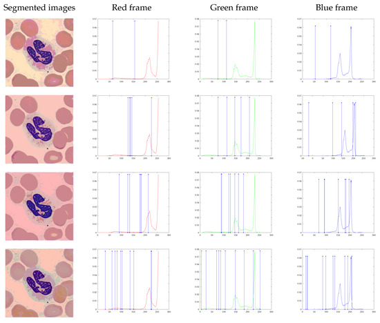
Figure 9. Threshold outcomes after executing mSAR on the Otsu method over the set of test images.

Table 8. mSAR Otsu in terms of fitness values competing overall for algorithms.

		LFD		HHO		SCA		EO		GSA		AOA		SAR		mSAR
Test Image	nTh	Mean	Std	Mean	Std	Mean	Std	Mean	Std	Mean	Std	Mean	Std	Mean	Std	Mean	Std
Test 1	2	1228.3380	1.3192E-15	2154.5265	1.3304E-15	2161.1633	1.2965E-15	1766.6759	1.4033E-03	2163.2565	1.2794E-15	2162.2380	9.2416E-02	2183.2334	1.1987E-15	2347.1712	1.1288E-15
	5	2267.7534	1.3192E-15	2336.1469	1.3304E-15	2344.7112	1.8691E-02	1766.6759	1.0255E-02	2345.5462	6.4323E-03	2325.5931	1.2796E-15	2368.7855	1.1987E-15	2417.2129	1.1288E-15
	7	2345.8176	9.1611E-04	2403.3510	3.9913E-15	2414.7995	5.5820E-03	1764.1485	2.2057E-02	2684.2501	5.3306E-04	2399.9273	8.1752E-04	2439.4421	3.5961E-15	2445.3025	3.3864E-15
	10	2433.4497	9.1611E-04	2429.4427	7.3173E-03	2443.2505	1.0120E-02	1762.3227	3.7421E-02	2848.9400	2.3490E-02	2439.9649	1.6741E-02	2466.6090	1.1987E-15	2468.1193	1.1288E-15
Test 2	2	2231.9467	1.3192E-15	2673.6262	1.3304E-15	2681.6200	1.2965E-15	2240.5229	6.1169E-04	2684.2501	1.2509E-14	2684.7420	1.2796E-15	2709.0176	1.1987E-15	2375.9160	1.1288E-15
	5	2256.1142	1.2716E-14	2838.4327	4.3978E-02	2847.5512	4.3215E-02	2245.7175	1.3421E-02	2849.5214	2.9887E-02	2844.4739	3.4229E-02	2876.6441	1.1987E-15	2413.1053	1.1288E-15
	7	2282.9820	5.7532E-05	2911.0919	5.6543E-05	2923.6189	3.9974E-02	2251.5354	2.4359E-02	2922.0748	2.1713E-04	2905.9256	1.1196E-01	2953.4878	4.7949E-15	2969.9479	4.5151E-15
	10	2389.8843	1.9055E-03	2955.3494	4.0652E-03	2966.8889	3.8174E-03	2266.9606	4.7496E-02	2921.9471	4.8687E-03	2969.5291	1.2121E-01	2997.2955	5.9936E-15	2998.4400	5.6439E-15
Test 3	2	1349.9321	1.3192E-15	1700.6816	1.3304E-15	1707.9356	1.2965E-15	1346.5997	3.0009E-04	1709.6107	3.8025E-14	1700.1406	1.2796E-15	1725.3852	1.1987E-15	1809.8735	1.1288E-15
	5	1436.6207	1.5647E-02	1800.7810	8.4999E-03	1808.0657	4.8257E-05	1368.6302	2.0869E-03	1869.1703	1.4784E-02	1793.0477	6.3980E-15	1826.5383	1.3818E-02	1869.1703	1.3012E-02
	7	1855.0663	1.3558E-03	1819.5871	7.3173E-02	1866.9733	1.6926E-03	1816.7927	3.3211E-02	1865.1461	6.8588E-02	1849.2056	5.2250E-02	1886.3811	2.4008E-15	1865.5869	2.2607E-15
	10	1883.8377	3.8843E-03	1883.7849	7.1695E-02	1895.8753	3.2772E-03	1855.9531	6.5486E-02	1864.1770	9.7728E-02	1885.1025	1.1943E-01	1915.1461	3.5961E-15	1917.1353	3.3864E-15
Test 4	2	3342.3522	5.2768E-15	4005.5150	5.3217E-15	4017.6015	1.1308E-06	3378.4302	9.3552E-04	4021.2621	5.1174E-15	4019.5170	5.1184E-15	4058.6485	4.7949E-15	4104.8147	4.9869E-15
	5	3357.6885	1.2313E-05	4087.9590	3.9913E-15	4100.7145	4.3215E-04	3532.9058	4.3897E-03	4104.5360	3.8381E-15	4104.5710	3.8388E-15	4142.5629	3.5961E-15	4165.3647	3.7402E-15
	7	3531.2658	1.2826E-04	4146.2650	1.8145E-04	4161.2052	1.5702E-04	3588.5685	1.2270E-02	4160.5588	5.3306E-04	4157.2434	6.6113E-05	4203.7193	1.1987E-15	4197.6941	1.2467E-15
	10	3566.7480	1.3962E-02	4180.4044	2.2913E-02	4195.6883	5.2939E-03	3628.7443	2.4755E-02	4192.1343	2.9247E-02	4221.9163	2.6943E-02	4229.6436	1.1987E-15	4221.8588	1.2467E-15
Test 5	2	2022.1883	1.3192E-15	2137.3286	1.3304E-15	2144.5158	1.2965E-15	2174.5007	3.1880E-04	2146.5530	1.0093E-14	2144.6728	1.2796E-15	2166.4247	1.1987E-15	2230.4867	1.2467E-15
	5	2105.3476	2.6970E-14	2220.8704	3.9913E-15	2228.2801	1.0120E-02	2205.3313	6.0449E-03	2229.1199	4.6199E-14	2216.7077	3.8388E-15	2251.0460	3.5961E-15	2280.5788	3.7402E-15
	7	2116.4290	7.6953E-04	2310.5996	9.9412E-02	2277.8903	5.9781E-02	2268.2821	6.0809E-02	2230.2398	7.2852E-02	2277.3147	9.5970E-02	2301.6064	5.9936E-15	2309.2243	6.1459E-15
	10	2205.3323	1.0370E-02	2295.5602	9.7934E-02	2306.9782	4.9698E-02	2311.4290	8.3837E-02	2275.9562	1.0128E-01	2257.8829	1.1090E-01	2338.5126	3.5961E-05	2325.0029	1.2292E-15
Test 6	2	2362.7631	2.6421E-15	2779.8693	2.6645E-15	2788.2653	2.5965E-15	2462.6670	5.3972E-04	2790.9999	2.5623E-15	2791.1473	2.5628E-15	2816.7524	2.4008E-15	2899.2436	2.4618E-15
	5	2543.9257	6.2295E-04	2986.4010	4.8782E-05	3026.3672	1.0444E-03	2696.2576	4.3178E-03	2999.7423	9.2398E-04	2969.9597	1.6919E-05	3026.3672	1.0988E-03	3010.8257	1.2292E-03
	7	2657.2510	2.3123E-04	3092.6749	2.6424E-02	3107.7510	3.2196E-04	2891.4927	2.5367E-02	3109.2573	2.5658E-02	3110.3556	4.4786E-02	3138.7965	5.9936E-15	3167.6023	6.1494E-15
	10	2673.9420	2.1620E-03	3150.4793	1.9587E-03	3164.3702	5.5460E-03	2919.2860	3.9580E-02	3115.0013	5.1885E-03	3166.8879	1.1445E-02	3196.6999	0.0000E+00	3201.8355	0.0000E+00
Test 7	2	1824.5625	1.3192E-15	1938.2958	8.7956E-05	1790.9441	5.2579E-05	1769.3905	1.2594E-03	1792.4297	7.5695E-05	1792.0819	4.0165E-05	1809.2418	1.1987E-15	1938.2958	1.2804E-15
	5	1835.9877	3.9576E-15	1928.5638	2.8752E-04	1936.3773	7.9228E-04	1917.0802	5.3253E-03	1935.5520	5.6860E-04	1939.3067	3.8388E-15	1956.1609	3.5961E-15	2014.0182	3.8412E-15
	7	1994.1837	3.6644E-04	1994.5436	2.8087E-03	2061.9455	2.8450E-03	1983.5858	1.5148E-02	2009.5965	2.2744E-03	2012.5464	1.8483E-03	2031.9621	8.3910E-15	2061.9455	8.9629E-15
	10	2002.4547	2.0521E-03	2045.0262	2.6608E-03	2089.0842	5.8701E-03	2033.1707	3.1772E-02	2008.9027	4.3000E-03	2053.9605	5.1539E-03	2080.4898	9.5897E-15	2091.3972	9.2998E-15
Test 8	2	3404.3880	5.2768E-15	3424.3880	5.3217E-15	3370.3381	3.7093E-05	2754.5731	4.6776E-03	3373.5875	5.1174E-15	3373.5524	1.5249E-01	3404.7155	4.7949E-15	3424.3880	4.6499E-15
	5	3447.8143	2.6970E-04	3520.6757	3.9913E-15	3534.2506	6.3383E-02	2918.6109	2.7814E-02	3536.3315	1.1017E-03	3537.8986	3.8388E-15	3570.3593	3.5961E-15	3599.4514	3.4874E-15
	7	3640.4737	6.9624E-04	3579.3755	1.2528E-04	3596.1054	1.8151E-02	2945.7964	4.3178E-02	3597.8396	1.0306E-03	3599.7578	6.3980E-04	3632.5749	3.5961E-15	3661.2643	3.4874E-15
	10	3557.6969	9.6008E-03	3692.4467	7.2434E-03	3638.5602	1.2749E-02	2963.2611	2.3892E-01	3626.7722	8.5646E-03	3618.3636	7.3577E-02	3675.7346	2.4008E-15	3692.4467	2.3282E-15

Table 9. mSAR Otsu in terms of PSNR values competed overall for algorithms.

		LFD		HHO		SCA		EO		GSA		AOA		SAR		mSAR
Test Image	nTh	Mean	Std	Mean	Std	Mean	Std	Mean	Std	Mean	Std	Mean	Std	Mean	Std	Mean	Std
Test 1	2	18.0774	5.2812E-14	18.0789	5.2380E-14	18.0789	5.2488E-14	18.0266	2.8130E-01	18.0600	5.2272E-14	18.0617	5.2380E-14	21.2302	5.2596E-14	19.0774	5.2488E-14
	5	21.2304	4.1076E-14	21.2322	7.0810E-02	21.2322	6.1722E-02	20.9442	7.5175E-01	21.2100	0.0000E+00	21.2120	0.0000E+00	22.1965	0.0000E+00	22.2304	0.0000E+00
	7	22.5967	1.9022E-14	22.5987	1.9061E-01	22.5987	2.0169E-01	22.0904	2.6675E+00	22.5750	3.4896E-14	22.5772	7.4205E-02	24.4883	3.5113E-14	24.5967	3.5041E-14
	10	24.4885	1.8778E-14	24.4906	9.9910E-02	24.4906	1.4677E-01	23.1324	3.5987E+00	24.4650	7.4052E-16	24.4673	1.0428E-01	24.1854	7.0128E-14	24.9885	6.9984E-14
Test 2	2	16.1856	3.5257E-14	16.1869	3.4969E-14	16.1869	3.5041E-14	16.0468	1.2028E-01	16.1700	3.4896E-14	16.1715	3.4969E-14	18.2874	3.5113E-14	16.1856	3.5041E-14
	5	18.2876	5.2812E-14	18.2891	8.0025E-02	18.2891	5.2488E-14	18.1308	4.9955E-01	18.2700	5.2272E-14	18.2717	5.2380E-14	19.7588	5.2596E-14	18.2876	5.2488E-14
	7	19.7590	1.9560E-16	19.7607	2.8615E-02	19.6556	1.1518E+00	19.0686	3.1186E+00	19.7400	0.0000E+00	19.7419	1.2125E-02	20.3894	0.0000E+00	19.7590	0.0000E+00
	10	20.4947	1.3839E-16	20.6016	1.5617E+00	20.3913	1.0012E+00	19.6938	2.8712E+00	20.4750	1.2826E+00	20.7920	1.7703E+00	20.1854	7.0128E-14	20.3896	6.9984E-14
Test 3	2	16.1856	6.1614E-14	18.6027	6.1110E-14	16.1869	6.1236E-14	16.0468	2.2456E-16	16.1700	6.0984E-14	16.1715	6.1110E-14	18.6027	6.1362E-14	16.1856	6.1236E-14
	5	18.6029	1.8093E-02	18.6045	3.0798E-01	18.6045	3.5041E-14	19.9350	3.8121E+00	18.5850	3.4896E-14	18.5868	1.3095E-02	19.2302	3.5113E-14	18.6029	3.5041E-14
	7	21.3355	1.7702E-01	21.2322	2.4347E-01	22.7616	2.0169E-01	20.2148	5.5775E+00	21.2100	7.1632E-16	21.2120	1.5569E-16	22.7016	5.2596E-14	21.2304	5.2488E-11
	10	22.8069	3.6920E-01	22.9140	9.6030E-01	22.7038	1.1713E+00	21.3610	6.1110E+00	22.6800	2.4200E-16	22.7872	4.8985E-01	22.8129	3.5113E-14	22.8918	3.5041E-14
Test 4	2	18.8131	0.0000E+00	21.3353	0.0000E+00	18.8147	0.0000E+00	18.6518	5.7715E-02	18.7950	0.0000E+00	18.7968	0.0000E+00	21.3353	0.0000E+00	18.8131	0.0000E+00
	5	21.3355	1.7702E-16	21.3373	4.4135E-02	21.3373	5.2488E-14	21.1526	3.5696E-01	21.3150	5.2272E-14	21.3170	5.2380E-14	22.3322	5.2596E-14	22.6355	5.2488E-13
	7	23.3324	6.3081E-02	23.3344	1.0573E-01	23.3344	3.8880E-02	23.0282	5.4805E-01	23.3100	2.4200E-16	23.3122	6.4020E-02	23.9087	3.5113E-14	23.4324	3.5041E-14
	10	24.9089	1.2959E-01	24.9111	8.4875E-02	24.9689	7.9218E-02	23.7576	3.4920E+00	24.8850	1.7424E-02	24.8874	6.4020E-16	24.7650	0.0000E+00	24.9689	0.0000E+00
Test 5	2	15.7652	6.1614E-14	15.7665	6.0140E-02	15.7665	6.1236E-14	15.6300	1.9982E-01	15.7500	6.0984E-14	15.7515	6.1110E-14	15.7588	6.1362E-14	16.7652	6.1236E-13
	5	19.7590	1.2616E-16	19.7607	2.9973E-01	19.7607	6.9984E-14	19.5896	1.4647E+00	19.7400	6.9696E-14	19.7419	1.3289E-01	19.7557	7.0128E-14	19.7590	6.9984E-14
	7	21.8610	1.6871E-16	21.8629	2.7063E-01	21.7578	9.3798E-02	21.1526	4.2923E+00	21.7350	5.2272E-14	21.7371	4.8500E-02	21.3832	5.2596E-14	22.7559	5.2488E-13
	10	24.2783	1.7653E+00	24.2804	1.8527E-01	24.1753	2.7070E+00	22.2988	4.8064E+00	24.3600	1.1132E-01	24.2573	1.4841E-01	24.1313	5.2596E-14	24.5834	5.2488E-14
Test 6	2	17.1315	5.2812E-14	17.1329	5.2380E-14	17.1329	6.9498E-04	16.9846	8.1480E-02	17.1150	5.2272E-14	17.1166	5.2380E-14	17.3384	5.2596E-14	17.1315	5.2488E-14
	5	19.3386	7.0416E-14	19.3402	2.2795E-02	19.3402	2.6341E-02	19.0686	1.6733E+00	19.3200	6.9696E-14	19.3218	6.9840E-14	19.7557	7.0128E-14	19.3386	6.9984E-14
	7	21.7559	4.8802E-16	21.7578	4.4620E-02	21.7578	1.2101E-01	20.7358	4.9955E+00	21.7350	1.3068E-02	21.7371	5.2380E-14	21.4373	5.2596E-14	21.7559	5.2488E-12
	10	23.4375	1.0269E-01	23.4395	8.2935E-02	23.4395	6.2694E-02	21.7778	4.3893E-16	23.4150	7.7440E-03	23.4172	5.4320E-02	23.8160	8.7660E-14	23.4375	8.7480E-14
Test 7	2	16.8162	2.6455E-14	16.8176	2.6239E-14	16.8176	2.6293E-14	16.6720	1.0234E-01	16.8000	2.6184E-14	16.8016	2.6239E-14	16.1282	2.6347E-14	17.8162	2.6293E-14
	5	19.1284	3.5257E-14	19.1300	4.6075E-02	19.1300	1.0595E-01	18.8602	1.8236E+00	19.1100	3.4896E-14	19.1118	3.4969E-14	19.7557	3.5113E-14	20.1284	3.5041E-14
	7	21.7559	9.3399E-16	21.7578	5.4320E-02	21.7578	1.4337E-01	20.8400	4.9470E+00	21.7350	8.7120E-14	21.7371	8.7300E-14	21.3322	8.7660E-14	21.9859	8.7480E-14
	10	23.3324	1.6528E-01	23.3344	1.2804E-01	23.3344	1.5260E-01	22.0904	4.2195E+00	23.3100	3.7268E-16	23.3122	2.5705E-02	23.4024	7.0128E-14	23.4024	6.9984E-14
Test 8	2	15.3447	0.0000E+00	15.3461	0.0000E+00	15.3461	0.0000E+00	15.2132	1.2125E-01	15.3300	0.0000E+00	15.3315	0.0000E+00	16.1792	0.0000E+00	15.3447	0.0000E+00
	5	20.1794	1.7604E-14	20.1811	1.7460E-14	20.1811	6.3180E-01	19.5896	6.0625E+00	20.1600	1.7424E-14	20.1619	1.7460E-14	20.2812	1.7532E-14	20.4794	1.7496E-14
	7	22.0712	3.7164E+00	22.1782	3.5114E-01	22.1782	6.8526E-01	19.1728	1.1786E+01	22.2600	2.4636E-01	22.2621	3.4969E-14	23.5424	3.5113E-14	23.6814	3.5041E-14
	10	23.3324	8.8020E-01	23.5826	1.2174E-01	23.4395	1.8760E+00	21.8820	7.5175E+00	23.5200	1.1084E-01	23.5222	1.6830E-01	23.3401	5.2596E-14	23.5826	5.2488E-14

Table 10. mSAR Otsu in terms of SSIM values overall competed for algorithms.

		LFD		HHO		SCA		EO		GSA		AOA		SAR		mSAR
Test Image	nTh	Mean	Std	Mean	Std	Mean	Std	Mean	Std	Mean	Std	Mean	Std	Mean	Std	Mean	Std
Test 1	2	0.8003	2.4625E-14	0.8010	1.9447E-15	0.8007	1.9628E-15	0.8009	6.2930E-03	0.8008	2.0079E-15	0.8008	1.9853E-15	0.8011	1.9575E-15	0.8010	1.9614E-15
	5	0.8409	3.1231E-03	0.8417	3.5876E-03	0.8414	3.7514E-04	0.8405	3.2613E-02	0.8415	3.5126E-15	0.8415	3.4732E-15	0.8418	3.4245E-15	0.8419	3.4314E-15
	7	0.8659	2.5061E-02	0.8667	2.3759E-03	0.8664	1.7060E-03	0.8624	2.4832E-02	0.8665	2.0079E-15	0.8665	9.8165E-04	0.8668	1.9575E-15	0.8672	1.9614E-15
	10	0.8940	5.1433E-02	0.8949	3.7514E-03	0.8946	2.3066E-03	0.8822	3.7970E-02	0.8946	9.0821E-03	0.8946	1.5891E-03	0.8950	1.4670E-15	0.8950	1.4700E-15
Test 2	2	0.6731	6.1698E-15	0.6738	4.8726E-16	0.6735	4.9178E-16	0.6747	8.8867E-03	0.6736	5.0308E-16	0.6736	4.9743E-16	0.6738	4.9045E-16	0.6738	4.9144E-16
	5	0.7523	2.4625E-14	0.7530	5.2606E-03	0.7528	1.9628E-15	0.7519	2.8361E-02	0.7528	2.0079E-15	0.7528	1.9853E-15	0.7531	1.9575E-15	0.7535	1.9614E-15
	7	0.7971	7.7532E-03	0.7980	7.5460E-04	0.7955	2.7635E-02	0.7842	9.0142E-02	0.7977	2.0079E-15	0.7977	4.4900E-04	0.7980	1.9575E-15	0.7980	1.9614E-15
	10	0.8221	5.1433E-01	0.8271	4.7001E-02	0.8205	3.9951E-02	0.8040	8.2489E-02	0.8237	3.9489E-02	0.8331	5.3704E-02	0.8199	9.7657E-16	0.8208	9.7853E-16
Test 3	2	0.8221	6.1698E-15	0.8235	4.8726E-16	0.8226	4.9178E-16	0.8228	1.0077E-02	0.8227	5.0308E-16	0.8227	4.9743E-16	0.8230	4.9045E-16	0.8235	4.9144E-16
	5	0.8899	2.2932E-03	0.8918	6.7698E-03	0.8904	3.4337E-15	0.8843	9.2268E-02	0.8905	3.5126E-15	0.8905	1.3250E-04	0.8908	3.4245E-15	0.8908	3.4314E-15
	7	0.9524	4.4663E-02	0.9523	4.9588E-03	0.9519	4.0735E-03	0.9323	1.1353E-01	0.9509	1.4647E-03	0.9520	3.2223E-03	0.9513	1.4670E-15	0.9513	1.4700E-15
	10	0.9732	6.4974E-02	0.9752	1.0909E-02	0.9727	1.5145E-02	0.9552	1.0502E-01	0.9728	3.0452E-04	0.9739	6.9552E-03	0.9732	2.4436E-15	0.9732	2.4485E-15
Test 4	2	0.7898	1.2285E-14	0.7906	9.7020E-16	0.7903	9.7920E-16	0.7904	3.7460E-03	0.7904	1.0017E-15	0.7904	9.9045E-16	0.7907	9.7657E-16	0.7907	9.7853E-16
	5	0.8826	2.1185E-02	0.8834	4.5707E-03	0.8831	2.4502E-15	0.8833	1.2543E-02	0.8832	2.5065E-15	0.8832	2.4783E-15	0.8832	2.4436E-15	0.8835	2.4485E-15
	7	0.9253	1.0483E-01	0.9272	1.3885E-02	0.9237	2.8636E-03	0.9291	3.0572E-02	0.9238	1.6517E-03	0.9270	1.2370E-02	0.9240	1.4670E-15	0.9242	1.4700E-15
	10	0.9607	2.1076E-02	0.9616	1.8240E-03	0.9613	9.9661E-04	0.9437	6.8457E-02	0.9614	2.9962E-04	0.9614	5.7226E-04	0.9616	2.4436E-15	0.9619	2.4485E-15
Test 5	2	0.8742	1.2285E-14	0.8751	1.8197E-03	0.8747	9.7920E-16	0.8760	6.6756E-03	0.8748	1.0017E-15	0.8748	9.9045E-16	0.8750	9.7657E-16	0.8752	9.7853E-16
	5	0.9274	9.0636E-02	0.9304	1.5998E-02	0.9269	9.7920E-16	0.9270	5.0174E-02	0.9270	1.0017E-15	0.9280	7.7475E-03	0.9271	9.7657E-16	0.9273	9.7853E-16
	7	0.9493	4.5482E-02	0.9502	5.3900E-03	0.9488	2.3718E-03	0.9458	5.1024E-02	0.9489	2.0079E-15	0.9489	1.2370E-03	0.9490	1.9575E-15	0.9502	1.9614E-15
	10	0.9836	2.7791E-01	0.9856	3.0874E-03	0.9842	3.5208E-02	0.9615	6.5906E-02	0.9864	2.1904E-03	0.9864	2.4387E-03	0.9866	4.9045E-16	0.9869	4.9144E-16
Test 6	2	0.7909	1.8455E-14	0.7919	1.4575E-15	0.7913	1.2229E-03	0.7915	5.9103E-03	0.7914	1.5048E-15	0.7914	1.4879E-15	0.7916	1.4670E-15	0.7919	1.4700E-15
	5	0.8326	0.0000E+00	0.8334	1.1039E-04	0.8330	2.5024E-03	0.8322	3.0062E-02	0.8331	0.0000E+00	0.8331	0.0000E+00	0.8333	0.0000E+00	0.8334	0.0000E+00
	7	0.8972	6.8796E-03	0.8980	3.1521E-04	0.8977	1.7452E-03	0.8739	1.1991E-01	0.8978	8.0581E-05	0.8978	0.0000E+00	0.8979	0.0000E+00	0.8986	0.0000E+00
	10	0.9211	2.1239E-02	0.9220	2.3630E-03	0.9217	6.8762E-04	0.9010	8.1213E-02	0.9217	3.7530E-04	0.9217	1.0213E-03	0.9219	2.4436E-15	0.9225	2.4485E-15
Test 7	2	0.7617	0.0000E+00	0.7624	0.0000E+00	0.7621	0.0000E+00	0.7623	5.0174E-03	0.7622	0.0000E+00	0.7622	0.0000E+00	0.7626	0.0000E+00	0.7626	0.0000E+00
	5	0.8419	1.2285E-14	0.8428	8.5378E-04	0.8414	1.8627E-03	0.8374	5.6126E-02	0.8425	1.0017E-15	0.8425	9.9045E-16	0.8427	9.7657E-16	0.8427	9.7853E-16
	7	0.9232	5.0942E-02	0.9241	4.0662E-03	0.9237	6.9632E-03	0.9031	1.3904E-01	0.9238	2.5065E-15	0.9238	2.4783E-15	0.9235	2.4436E-15	0.9243	2.4485E-15
	10	0.9597	7.9170E-02	0.9585	6.3818E-03	0.9581	6.3539E-03	0.9364	9.9072E-02	0.9572	2.4531E-04	0.9572	4.2347E-03	0.9568	0.0000E+00	0.9575	0.0000E+00
Test 8	2	0.7304	2.4625E-14	0.7310	1.9447E-15	0.7309	1.9628E-15	0.7300	5.1874E-03	0.7309	2.0079E-15	0.7309	1.9853E-15	0.7307	1.9575E-15	0.7318	1.9614E-15
	5	0.9201	1.2285E-14	0.9210	9.7020E-16	0.9206	1.2055E-02	0.9062	2.0197E-01	0.9207	1.0017E-15	0.9207	9.9045E-16	0.9204	9.7657E-16	0.9210	9.7853E-16
	7	0.9566	1.1630E+00	0.9616	2.9839E-03	0.9613	8.7910E-03	0.8791	3.1167E-01	0.9624	1.8921E-03	0.9624	4.9743E-16	0.9620	4.9045E-16	0.9627	4.9144E-16
	10	0.9795	1.4360E-01	0.9826	1.6213E-03	0.9800	2.0846E-02	0.9521	1.7051E-01	0.9822	1.0907E-03	0.9822	1.6948E-03	0.9818	2.4436E-15	0.9825	2.4485E-15

Table 11. mSAR Otsu in terms of FSIM values overall competed for algorithms.

		LFD		HHO		SCA		EO		GSA		AOA		SAR		mSAR
Test Image	nTh	Mean	Std	Mean	Std	Mean	Std	Mean	Std	Mean	Std	Mean	Std	Mean	Std	Mean	Std
Test 1	2	0.8005	1.9063E-15	0.8005	1.8725E-15	0.8005	1.8759E-15	0.8006	1.0805E-02	0.7997	1.9401E-15	0.7982	1.9131E-15	0.8005	1.8725E-15	0.8002	1.8759E-15
	5	0.8457	8.9112E-05	0.8457	1.6354E-03	0.8457	1.3209E-04	0.8458	1.2488E-15	0.8449	1.2915E-15	0.8433	1.2735E-15	0.8457	1.2465E-15	0.8418	1.2488E-15
	7	0.8789	5.1117E-03	0.8794	3.6486E-03	0.8795	4.2458E-03	0.8800	3.1247E-15	0.8790	3.2316E-15	0.8773	1.8343E-03	0.8799	3.1190E-15	0.8691	3.1247E-15
	10	0.9199	3.1590E-03	0.9202	1.6471E-03	0.9202	2.5890E-03	0.9202	9.6348E-15	0.9188	1.4372E-02	0.9173	1.5747E-03	0.9200	4.3711E-15	0.9201	4.3790E-15
Test 2	2	0.7249	1.9063E-15	0.7249	1.8725E-15	0.7249	1.8759E-15	0.7232	8.1872E-03	0.7243	1.9401E-15	0.7229	1.9131E-15	0.7249	1.8725E-15	0.7250	1.8759E-15
	5	0.7823	1.2690E-15	0.7825	4.2585E-03	0.7823	1.2488E-15	0.7791	2.8914E-02	0.7815	1.2915E-15	0.7800	1.2735E-15	0.7823	1.2465E-15	0.7824	1.2488E-15
	7	0.8340	1.6652E-03	0.8339	2.5451E-03	0.8313	6.0495E-02	0.8343	1.2718E-01	0.8334	1.9401E-15	0.8317	1.1600E-03	0.8346	1.8725E-15	0.8341	1.8759E-15
	10	0.8636	3.8757E-02	0.8647	4.2679E-03	0.8631	3.8261E-02	0.8652	9.8151E-02	0.8640	2.5572E-03	0.8622	3.7751E-03	0.8651	1.8725E-15	0.8652	1.8759E-15
Test 3	2	0.8774	6.3732E-16	0.8774	6.2602E-16	0.8774	6.2715E-16	0.8775	9.4338E-03	0.8766	6.4862E-16	0.8749	6.3958E-16	0.8774	6.2602E-16	0.8773	6.2715E-16
	5	0.9216	2.4545E-03	0.9212	5.0238E-03	0.9219	4.3790E-15	0.9218	7.5124E-15	0.9208	4.5289E-15	0.9190	1.7679E-03	0.9217	4.3711E-15	0.9216	4.3790E-15
	7	0.9596	2.9326E-03	0.9589	4.3127E-03	0.9589	3.4143E-03	0.9587	9.7989E-15	0.9578	1.2119E-03	0.9561	2.6252E-03	0.9586	1.8725E-15	0.9583	1.8759E-15
	10	0.9764	5.3657E-03	0.9757	5.6087E-03	0.9752	1.5189E-02	0.9756	9.9618E-15	0.9746	2.0514E-03	0.9734	5.8309E-03	0.9755	3.1190E-15	0.9750	3.1247E-15
Test 4	2	0.8255	2.5436E-15	0.8255	2.4985E-15	0.8255	2.5031E-15	0.8256	1.6323E-11	0.8247	2.5887E-15	0.8231	2.5527E-15	0.8255	2.4985E-15	0.8256	2.5031E-15
	5	0.9068	6.3732E-04	0.9066	1.6067E-03	0.9068	3.1247E-15	0.9069	3.3932E-03	0.9059	3.2316E-15	0.9042	3.1866E-15	0.9068	3.1190E-15	0.9065	3.1247E-15
	7	0.9464	2.2175E-03	0.9464	2.7302E-03	0.9460	1.5152E-03	0.9461	9.9742E-03	0.9451	5.1660E-04	0.9437	2.2139E-03	0.9460	3.1190E-15	0.9459	3.1247E-15
	10	0.9733	1.5789E-03	0.9730	8.4385E-04	0.9729	2.8749E-04	0.9730	7.4054E-02	0.9720	3.7540E-04	0.9720	1.0920E-03	0.9729	2.4985E-15	0.9724	2.5031E-15
Test 5	2	0.8418	1.2690E-15	0.8419	2.0188E-03	0.8418	1.2488E-15	0.8419	5.3380E-06	0.8410	1.2915E-15	0.8410	1.2735E-15	0.8418	1.2465E-15	0.8419	1.2488E-15
	5	0.8828	5.4885E-03	0.8839	1.2167E-02	0.8823	6.2715E-16	0.8839	3.5241E-02	0.8815	6.4862E-16	0.8820	5.8456E-03	0.8823	6.2602E-16	0.8824	6.2715E-16
	7	0.9187	6.2006E-03	0.9192	8.3615E-03	0.9182	3.0137E-03	0.9195	8.3266E-02	0.9171	1.9401E-15	0.9172	2.5535E-03	0.9180	1.8725E-15	0.9181	1.8759E-15
	10	0.9508	2.9314E-02	0.9519	5.1383E-03	0.9507	4.3045E-02	0.9528	9.2372E-02	0.9515	3.8453E-03	0.9515	3.7680E-03	0.9528	2.4985E-15	0.9523	2.5031E-15
Test 6	2	0.7520	1.9063E-15	0.7520	1.8725E-15	0.7520	2.8971E-04	0.7489	2.3302E-03	0.7513	1.9401E-15	0.7513	1.9131E-15	0.7520	1.8725E-15	0.7521	1.8759E-15
	5	0.8108	1.9063E-15	0.8107	4.4874E-04	0.8107	1.1600E-03	0.8063	5.5225E-02	0.8100	1.9401E-15	0.8100	1.9131E-15	0.8109	1.8725E-15	0.8109	1.8759E-15
	7	0.8548	1.3085E-03	0.8546	6.5721E-04	0.8549	1.6151E-03	0.8350	1.0860E-01	0.8538	3.5703E-04	0.8538	4.4657E-15	0.8546	4.3711E-15	0.8547	4.3790E-15
	10	0.8905	2.0094E-03	0.8906	3.1786E-03	0.8902	8.0475E-04	0.8569	1.1039E-01	0.8892	1.5441E-04	0.8894	1.3569E-03	0.8901	1.2465E-15	0.8909	1.2488E-15
Test 7	2	0.7860	2.5436E-15	0.7860	2.4985E-15	0.7860	2.5031E-15	0.7829	2.9645E-03	0.7853	2.5887E-15	0.7853	2.5527E-15	0.7860	2.4985E-15	0.7861	2.5031E-15
	5	0.8603	1.2690E-15	0.8603	7.8114E-05	0.8603	7.5480E-04	0.8530	6.7329E-02	0.8595	1.2915E-15	0.8603	1.2735E-15	0.8603	1.2465E-15	0.8604	1.2488E-15
	7	0.9169	7.3884E-04	0.9167	2.5547E-03	0.9167	3.5132E-03	0.8970	1.2209E-01	0.9159	1.9401E-15	0.9168	1.9131E-15	0.9168	1.8725E-15	0.9169	1.8759E-15
	10	0.9476	5.6896E-03	0.9464	5.2097E-03	0.9462	5.8231E-03	0.9223	1.0201E-01	0.9447	1.1114E-03	0.9458	3.9644E-03	0.9456	3.1190E-15	0.9479	3.1247E-15
Test 8	2	0.7862	1.2690E-15	0.7862	1.2465E-15	0.7862	1.2488E-15	0.7864	2.7730E-13	0.7854	1.2915E-15	0.7862	1.2735E-15	0.7864	1.2465E-15	0.7862	1.2488E-15
	5	0.8668	2.5436E-15	0.8668	2.4985E-15	0.8669	7.2150E-03	0.8669	1.1402E-08	0.8660	2.5887E-15	0.8668	2.5527E-15	0.8668	2.4985E-15	0.8669	2.5031E-15
	7	0.9252	5.4428E-02	0.9278	4.6802E-03	0.9270	5.2637E-03	0.9276	1.8180E-07	0.9267	3.3973E-03	0.9275	0.0000E+00	0.9275	0.0000E+00	0.9276	0.0000E+00
	10	0.9618	3.0370E-02	0.9632	1.7366E-03	0.9618	2.7877E-02	0.9635	9.9484E-08	0.9625	6.9115E-04	0.9633	1.0963E-03	0.9634	6.2602E-16	0.9635	6.2715E-16

The mean and STD of fitness outcomes obtained by the mSAR algorithm and other completed algorithms for all test images are shown in Table 8. The proposed mSAR algorithm comes in the first position with 22 higher fitness values in 32 experiments, followed by the original SAR in the second position with seven experiments, and HHO in the third position with four experiments. However, GSA comes in at the fourth position with three experiments, and SCA obtains the fifth position with only two experiments. The remaining algorithms, LFD, EO, and AOA, finish last with no experiments. The values of STD computed for each of the benchmark images with a different number of thresholds are shown in Table 8, and the algorithm is less stable when the value of STD is higher. According to the values of the STD, HHO comes in the first position, while the mSAR and SAR come in the second position, followed by LFD. AOA comes in the fourth position, and the GSA takes the fifth position. The final algorithms, SCA and EO, come in the last position.

Table 9 illustrates the Mean and STD of the PSNR outcomes for all test images, the optimal outcomes obtained are highlighted in bold. It is noticed that the mSAR displayed superiority in MTH after obtaining optimal PSNR values for 17 cases from 32 experiments. The original SAR obtains the second position with nine experiments, while HHO comes in the third position with seven experiments, followed by SCA in the fourth position with six experiments. However, the AOA and EO rank fifth with only one experiment, while the GSA and LFD come in last with no experiments. According to the values of STD, LFD is in the first position, followed by GSA. However, the original SAR comes in third place, while mSAR comes in fourth position. AOA comes in the fifth position, while the SCA and HHO come in the sixth position. In the end, the EO comes in the last position with the highest value of STD and a less stable algorithm.

In Table 10, the outcomes of the mean and STD values of SSIM obtained by the proposed mSAR and other completed algorithms are presented, and the optimal results are noted in bold. The outcomes indicate that mSAR is in the first position for twenty-one cases from thirty-two experiments in terms of the SSIM. The HHO is in the second position with eleven experiments, while the original SAR comes in the third position with four experiments. However, the EO obtains the fourth position with three experiments, followed by the LFD in the fifth position with only two experiments. Finally, the remaining algorithms, SCA, GSA, and AOA, come in the last position, without any experiments. The original SAR and mSAR algorithms are the best stable algorithms because their STD values are lower in most experiments, while GSA comes in the second position followed by AOA. However, SCA and HHO obtain the fourth position, and LFD comes in the fifth position. Finally, due to its high STD values in the majority of experiments, EO is the most unstable algorithm.

The mean and STD of the FSIM outcomes for all test images are displayed in Table 11, and the optimal outcomes are highlighted in bold. According to the outcomes of the FSIM, the EO comes in the first position with fifteen cases from thirty-two experiments, followed by mSAR in the second position with thirteen higher cases. HHO comes in the third position with six experiments, while the LFD is in the fourth position with five experiments. However, the original SAR obtained the fifth position with four experiments, and the SCA came in the sixth position with only three experiments. Finally, GSA and AOA come in last, without any experiments. According to the STD values, GSA comes in the first position, followed by the original SAR and mSAR in the second position. However, LFD obtains the third position, and AOA comes in the fourth position. EO comes in the fifth position, while the remaining algorithms, SCA and HHO, come in last, with less stable algorithms.

The outcomes of the Wilcoxon rank-sum test for fitness using the Otsu method as an objective function are shown in Table A4 of Appendix A. During execution of the Wilcoxon rank-sum test between mSAR and the following algorithms (LFD, HHO, SCA, EO, GSA, AOA, and SAR), it was noticed that there was a difference between the proposed mSAR algorithm and the other competing algorithms. This difference indicates that the proposed mSAR algorithm has undergone significant development. However, when compared to the EO and SAR, it is clear that they have comparable behavior, as noticed in tables with $(p>0.05)$ or NaN values. According to previous results, the results of the mSAR algorithm in the Fuzzy Entropy method are better than the results of the Otsu method, especially in $nTh=7$. Additionally, the quality of segmented color images using the fuzzy entropy method is high, as shown in Figure 8.

5.6. The Pros and Cons of the mSAR Algorithm

This subsection discusses the benefits and downsides of the proposed mSAR algorithm. The main benefits of the proposed mSAR can be summarized as its ease of implementation and understanding. The proposed mSAR algorithm has proven superior in solving color image-segmentation problems when compared to competing algorithms and gives good outcomes in terms of the quality of the segmented images.Furthermore, the mSAR produces a high convergence speed, indicating that the mSAR avoids entrapping in local optima and successfully balances the interchange between exploration and exploitation phases, owing to the fast finding of the threshold values and the high accuracy of the outcomes. The main defect of the mSAR is that the proposed algorithm is simple but computationally expensive. Additionally, the outcomes of STD values are not good enough to compete with the other algorithms.

6. Conclusions and Future Work

This paper presents an improved version of the SAR algorithm utilizing the concept of the OBL technique called mSAR. OBL improves the searchability of the original SAR, enables it to avoid entrapping in local optima, and successfully balances between the exploration and exploitation phases. mSAR is utilized to segment blood cell images and solve the problems of multi-level thresholding for image segmentation. IEEE CEC’2020 benchmark functions are utilized to prove the sturdiness of mSAR, and the proposed mSAR is implemented on a real application and executed as a multi-level image segmentation tool for estimating its performance on a set of color blood images. The proposed algorithm utilized fuzzy entropy and Otsu methods as objective functions to determine the optimal thresholds during the segmentation processes. The outcomes of the experiment proved the superiority of the proposed mSAR algorithm in producing good segmentation performance to segment the blood images and solve the CEC’2020 benchmark functions compared with other optimization algorithms. In future work, the proposed mSAR can be utilized to track the size of blood cells and tackle different problems such as feature selection, parameter identification, and task scheduling.

References

- Merzban, M.H.; Elbayoumi, M. Efficient solution of Otsu multilevel image thresholding: A comparative study. Expert Syst. Appl. 2019, 116, 299–309. [Google Scholar] [CrossRef]
- Bhandari, A.K.; Singh, V.K.; Kumar, A.; Singh, G.K. Cuckoo search algorithm and wind driven optimization based study of satellite image segmentation for multilevel thresholding using Kapur’s entropy. Expert Syst. Appl. 2014, 41, 3538–3560. [Google Scholar] [CrossRef]
- Sanei, S.H.R.; Fertig III, R.S. Uncorrelated volume element for stochastic modeling of microstructures based on local fiber volume fraction variation. Compos. Sci. Technol. 2015, 117, 191–198. [Google Scholar] [CrossRef]
- Sarkar, S.; Sen, N.; Kundu, A.; Das, S.; Chaudhuri, S.S. A differential evolutionary multilevel segmentation of near infra-red images using Renyi’s entropy. In Proceedings of the International Conference on Frontiers of Intelligent Computing: Theory and Applications (FICTA), Odisha, India, 22–23 December 2013; Springer: Berlin/Heidelberg, Germany, 2013; pp. 699–706. [Google Scholar]
- Houssein, E.H.; Helmy, B.E.d.; Oliva, D.; Jangir, P.; Premkumar, M.; Elngar, A.A.; Shaban, H. An efficient multi-thresholding based COVID-19 CT images segmentation approach using an improved equilibrium optimizer. Biomed. Signal Process. Control 2022, 73, 103401. [Google Scholar] [CrossRef]
- Abd El Aziz, M.; Ewees, A.A.; Hassanien, A.E. Whale optimization algorithm and moth-flame optimization for multilevel thresholding image segmentation. Expert Syst. Appl. 2017, 83, 242–256. [Google Scholar] [CrossRef]
- Houssein, E.H.; Sayed, A. Dynamic Candidate Solution Boosted Beluga Whale Optimization Algorithm for Biomedical Classification. Mathematics 2023, 11, 707. [Google Scholar] [CrossRef]
- Houssein, E.H.; Saad, M.R.; Hashim, F.A.; Shaban, H.; Hassaballah, M. Lévy flight distribution: A new metaheuristic algorithm for solving engineering optimization problems. Eng. Appl. Artif. Intell. 2020, 94, 103731. [Google Scholar] [CrossRef]
- Houssein, E.H.; Mahdy, M.A.; Eldin, M.G.; Shebl, D.; Mohamed, W.M.; Abdel-Aty, M. Optimizing quantum cloning circuit parameters based on adaptive guided differential evolution algorithm. J. Adv. Res. 2021, 29, 147–157. [Google Scholar] [CrossRef]
- Houssein, E.H.; Emam, M.M.; Ali, A.A.; Suganthan, P.N. Deep and machine learning techniques for medical imaging-based breast cancer: A comprehensive review. Expert Syst. Appl. 2021, 167, 114161. [Google Scholar] [CrossRef]
- Houssein, E.H.; Hosney, M.E.; Oliva, D.; Mohamed, W.M.; Hassaballah, M. A novel hybrid Harris hawks optimization and support vector machines for drug design and discovery. Comput. Chem. Eng. 2020, 133, 106656. [Google Scholar] [CrossRef]
- Houssein, E.H.; Saad, M.R.; Hussain, K.; Zhu, W.; Shaban, H.; Hassaballah, M. Optimal sink node placement in large scale wireless sensor networks based on Harris’ hawk optimization algorithm. IEEE Access 2020, 8, 19381–19397. [Google Scholar] [CrossRef]
- Abualigah, L.; Al-Okbi, N.K.; Elaziz, M.A.; Houssein, E.H. Boosting Marine Predators Algorithm by Salp Swarm Algorithm for Multilevel Thresholding Image Segmentation. Multimed. Tools Appl. 2022, 81, 16707–16742. [Google Scholar] [CrossRef] [PubMed]
- Neggaz, N.; Houssein, E.H.; Hussain, K. An efficient henry gas solubility optimization for feature selection. Expert Syst. Appl. 2020, 152, 113364. [Google Scholar] [CrossRef]
- Hashim, F.A.; Houssein, E.H.; Mabrouk, M.S.; Al-Atabany, W.; Mirjalili, S. Henry gas solubility optimization: A novel physics-based algorithm. Future Gener. Comput. Syst. 2019, 101, 646–667. [Google Scholar] [CrossRef]
- Hashim, F.A.; Hussain, K.; Houssein, E.H.; Mabrouk, M.S.; Al-Atabany, W. Archimedes optimization algorithm: A new metaheuristic algorithm for solving optimization problems. Appl. Intell. 2020, 51, 1531–1551. [Google Scholar] [CrossRef]
- Eberhart, R.C.; Shi, Y. Comparison between genetic algorithms and particle swarm optimization. In Proceedings of the International Conference on Evolutionary Programming, San Diego, CA, USA, 25–27 March 1998; Springer: Berlin/Heidelberg, Germany, 1998; pp. 611–616. [Google Scholar]
- Eberhart, R.; Kennedy, J. A new optimizer using particle swarm theory. In Proceedings of the MHS’95 Sixth International Symposium on Micro Machine and Human Science, Nagoya, Japan, 4–6 October 1995; IEEE: Piscataway, NJ, USA, 1995; pp. 39–43. [Google Scholar]
- Deb, K. Multi-objective optimisation using evolutionary algorithms: An introduction. In Multi-Objective Evolutionary Optimisation for Product Design and Manufacturing; Springer: Berlin/Heidelberg, Germany, 2011; pp. 3–34. [Google Scholar]
- Holland, J.H. Genetic algorithms. Sci. Am. 1992, 267, 66–73. [Google Scholar] [CrossRef]
- Storn, R.; Price, K. Differential evolution–a simple and efficient heuristic for global optimization over continuous spaces. J. Glob. Optim. 1997, 11, 341–359. [Google Scholar] [CrossRef]
- Heidari, A.A.; Mirjalili, S.; Faris, H.; Aljarah, I.; Mafarja, M.; Chen, H. Harris hawks optimization: Algorithm and applications. Future Gener. Comput. Syst. 2019, 97, 849–872. [Google Scholar] [CrossRef]
- Lv, W.; He, C.; Li, D.; Cheng, S.; Luo, S.; Zhang, X. Election campaign optimization algorithm. Procedia Comput. Sci. 2010, 1, 1377–1386. [Google Scholar] [CrossRef]
- Rao, R.V.; Savsani, V.J.; Vakharia, D. Teaching–learning-based optimization: A novel method for constrained mechanical design optimization problems. Comput. Aided Des. 2011, 43, 303–315. [Google Scholar] [CrossRef]
- Birbil, Ş.İ.; Fang, S.C. An electromagnetism-like mechanism for global optimization. J. Glob. Optim. 2003, 25, 263–282. [Google Scholar] [CrossRef]
- Rashedi, E.; Nezamabadi-Pour, H.; Saryazdi, S. GSA: A gravitational search algorithm. Inf. Sci. 2009, 179, 2232–2248. [Google Scholar] [CrossRef]
- Houssein, E.H.; El-dinHelmy, B.; Oliva, D.; Elngar, A.A.; Shabana, H. A novel Black Widow Optimization algorithm for multilevel thresholding image segmentation. Expert Syst. Appl. 2021, 167, 114159. [Google Scholar] [CrossRef]
- Dhal, K.G.; Das, A.; Ray, S.; Gálvez, J.; Das, S. Nature-inspired optimization algorithms and their application in multi-thresholding image segmentation. Arch. Comput. Methods Eng. 2020, 27, 855–888. [Google Scholar]
- Zhou, Y.; Yang, X.; Ling, Y.; Zhang, J. Meta-heuristic moth swarm algorithm for multilevel thresholding image segmentation. Multimed. Tools Appl. 2018, 77, 23699–23727. [Google Scholar] [CrossRef]
- Zhao, D.; Liu, L.; Yu, F.; Heidari, A.A.; Wang, M.; Oliva, D.; Muhammad, K.; Chen, H. Ant colony optimization with horizontal and vertical crossover search: Fundamental visions for multi-threshold image segmentation. Expert Syst. Appl. 2021, 167, 114122. [Google Scholar]
- He, L.; Huang, S. Modified firefly algorithm based multilevel thresholding for color image segmentation. Neurocomputing 2017, 240, 152–174. [Google Scholar] [CrossRef]
- Houssein, E.H.; Emam, M.M.; Ali, A.A. Improved manta ray foraging optimization for multi-level thresholding using COVID-19 CT images. Neural Comput. Appl. 2021, 33, 16899–16919. [Google Scholar] [CrossRef]
- Houssein, E.H.; Emam, M.M.; Ali, A.A. An optimized deep learning architecture for breast cancer diagnosis based on improved marine predators algorithm. Neural Comput. Appl. 2022, 34, 18015–18033. [Google Scholar] [CrossRef]
- Houssein, E.H.; Emam, M.M.; Ali, A.A. An efficient multilevel thresholding segmentation method for thermography breast cancer imaging based on improved chimp optimization algorithm. Expert Syst. Appl. 2021, 185, 115651. [Google Scholar] [CrossRef]
- Abd Elaziz, M.; Ewees, A.A.; Oliva, D. Hyper-heuristic method for multilevel thresholding image segmentation. Expert Syst. Appl. 2020, 146, 113201. [Google Scholar] [CrossRef]
- He, L.; Huang, S. An efficient krill herd algorithm for color image multilevel thresholding segmentation problem. Appl. Soft Comput. 2020, 89, 106063. [Google Scholar] [CrossRef]
- Bao, X.; Jia, H.; Lang, C. A novel hybrid harris hawks optimization for color image multilevel thresholding segmentation. IEEE Access 2019, 7, 76529–76546. [Google Scholar] [CrossRef]
- Shabani, A.; Asgarian, B.; Salido, M.; Gharebaghi, S.A. Search and rescue optimization algorithm: A new optimization method for solving constrained engineering optimization problems. Expert Syst. Appl. 2020, 161, 113698. [Google Scholar] [CrossRef]
- Rojas-Morales, N.; Rojas, M.C.R.; Ureta, E.M. A survey and classification of opposition-based metaheuristics. Comput. Ind. Eng. 2017, 110, 424–435. [Google Scholar] [CrossRef]
- Tizhoosh, H.R. Opposition-based learning: A new scheme for machine intelligence. In Proceedings of the International Conference on Computational Intelligence for Modelling, Control and Automation and International Conference on Intelligent Agents, Web Technologies and Internet Commerce (CIMCA-IAWTIC’06), Vienna, Austria, 28–30 November 2005; IEEE: Piscataway, NJ, USA, 2005; Volume 1, pp. 695–701. [Google Scholar]
- Chakraborty, F.; Roy, P.K.; Nandi, D. Oppositional elephant herding optimization with dynamic Cauchy mutation for multilevel image thresholding. Evol. Intell. 2019, 12, 445–467. [Google Scholar] [CrossRef]
- Houssein, E.H.; Hussain, K.; Abualigah, L.; Abd Elaziz, M.; Alomoush, W.; Dhiman, G.; Djenouri, Y.; Cuevas, E. An improved opposition-based marine predators algorithm for global optimization and multilevel thresholding image segmentation. Knowl. Based Syst. 2021, 229, 107348. [Google Scholar] [CrossRef]
- Gupta, S.; Deep, K.; Heidari, A.A.; Moayedi, H.; Wang, M. Opposition-based Learning Harris Hawks Optimization with Advanced Transition Rules: Principles and Analysis. Expert Syst. Appl. 2020, 158, 113510. [Google Scholar] [CrossRef]
- Gupta, S.; Deep, K. A hybrid self-adaptive sine cosine algorithm with opposition based learning. Expert Syst. Appl. 2019, 119, 210–230. [Google Scholar] [CrossRef]
- Ewees, A.A.; Abd Elaziz, M.; Oliva, D. A new multi-objective optimization algorithm combined with opposition-based learning. Expert Syst. Appl. 2021, 165, 113844. [Google Scholar] [CrossRef]
- Ewees, A.A.; Elaziz, M.A.; Houssein, E.H. Improved grasshopper optimization algorithm using opposition-based learning. Expert Syst. Appl. 2018, 112, 156–172. [Google Scholar] [CrossRef]
- Fan, Q.; Huang, H.; Yang, K.; Zhang, S.; Yao, L.; Xiong, Q. A modified equilibrium optimizer using opposition-based learning and novel update rules. Expert Syst. Appl. 2021, 170, 114575. [Google Scholar] [CrossRef]
- Sharma, T.K.; Pant, M. Opposition based learning ingrained shuffled frog-leaping algorithm. J. Comput. Sci. 2017, 21, 307–315. [Google Scholar] [CrossRef]
- Remli, M.A.; Deris, S.; Mohamad, M.S.; Omatu, S.; Corchado, J.M. An enhanced scatter search with combined opposition-based learning for parameter estimation in large-scale kinetic models of biochemical systems. Eng. Appl. Artif. Intell. 2017, 62, 164–180. [Google Scholar] [CrossRef]
- Naidu, M.; Kumar, P.R.; Chiranjeevi, K. Shannon and fuzzy entropy based evolutionary image thresholding for image segmentation. Alex. Eng. J. 2018, 57, 1643–1655. [Google Scholar] [CrossRef]
- Otsu, N. A threshold selection method from gray-level histograms. IEEE Trans. Syst. Man Cybern. 1979, 9, 62–66. [Google Scholar] [CrossRef]
- De Luca, A.; Termini, S. A definition of a nonprobabilistic entropy in the setting of fuzzy sets theory. Inf. Control 1972, 20, 301–312. [Google Scholar] [CrossRef]
- Mohamed, A.W.; Hadi, A.A.; Mohamed, A.K.; Awad, N.H. Evaluating the Performance of Adaptive GainingSharing Knowledge Based Algorithm on CEC 2020 Benchmark Problems. In Proceedings of the 2020 IEEE Congress on Evolutionary Computation (CEC), Glasgow, UK, 19–24 July 2020; IEEE: Piscataway, NJ, USA, 2020; pp. 1–8. [Google Scholar]
- Delgado-Ortet, M.; Molina, A.; Alférez, S.; Rodellar, J.; Merino, A. A deep learning approach for segmentation of red blood cell images and malaria detection. Entropy 2020, 22, 657. [Google Scholar] [CrossRef]
- Mirjalili, S. SCA: A sine cosine algorithm for solving optimization problems. Knowl. Based Syst. 2016, 96, 120–133. [Google Scholar] [CrossRef]
- Faramarzi, A.; Heidarinejad, M.; Stephens, B.; Mirjalili, S. Equilibrium optimizer: A novel optimization algorithm. Knowl. Based Syst. 2020, 191, 105190. [Google Scholar] [CrossRef]
- Abualigah, L.; Diabat, A.; Mirjalili, S.; Abd Elaziz, M.; Gandomi, A.H. The arithmetic optimization algorithm. Comput. Methods Appl. Mech. Eng. 2021, 376, 113609. [Google Scholar] [CrossRef]
- Oliva, D.; Cuevas, E.; Pajares, G.; Zaldivar, D.; Osuna, V. A multilevel thresholding algorithm using electromagnetism optimization. Neurocomputing 2014, 139, 357–381. [Google Scholar] [CrossRef]
- Huynh-Thu, Q.; Ghanbari, M. Scope of validity of PSNR in image/video quality assessment. Electron. Lett. 2008, 44, 800–801. [Google Scholar] [CrossRef]
- Yin, P.Y. Multilevel minimum cross entropy threshold selection based on particle swarm optimization. Appl. Math. Comput. 2007, 184, 503–513. [Google Scholar] [CrossRef]
- Wang, Z.; Bovik, A.C.; Sheikh, H.R.; Simoncelli, E.P. Image quality assessment: From error visibility to structural similarity. IEEE Trans. Image Process. 2004, 13, 600–612. [Google Scholar] [CrossRef]
- Arbelaez, P.; Maire, M.; Fowlkes, C.; Malik, J. Contour detection and hierarchical image segmentation. IEEE Trans. Pattern Anal. Mach. Intell. 2010, 33, 898–916. [Google Scholar] [CrossRef]
- Wilcoxon, F. Individual comparisons by ranking methods. In Breakthroughs in Statistics; Springer: Berlin/Heidelberg, Germany, 1992; pp. 196–202. [Google Scholar]
- Friedman, M. A comparison of alternative tests of significance for the problem of m rankings. Ann. Math. Stat. 1940, 11, 86–92. [Google Scholar] [CrossRef]
Disclaimer/Publisher’s Note: The statements, opinions and data contained in all publications are solely those of the individual author(s) and contributor(s) and not of MDPI and/or the editor(s). MDPI and/or the editor(s) disclaim responsibility for any injury to people or property resulting from any ideas, methods, instructions or products referred to in the content. |
© 2023 by the authors. Licensee MDPI, Basel, Switzerland. This article is an open access article distributed under the terms and conditions of the Creative Commons Attribution (CC BY) license (https://creativecommons.org/licenses/by/4.0/).