Tool Wear Detection in Milling Using Convolutional Neural Networks and Audible Sound Signals

Abstract

Timely tool wear detection has been an important target for the metal cutting industry for decades because of its significance for part quality and production cost control. With the shift toward intelligent and sustainable manufacturing, reliable tool-condition monitoring has become even more critical. One of the main challenges in sound-based tool wear monitoring is the presence of noise interference, instability and the highly volatile nature of machining acoustics, which complicates the extraction of meaningful features. In this study, a Convolutional Neural Network (CNN) model is proposed to classify tool wear conditions in milling operations using acoustic signals. Sound recordings were collected from tools at different wear stages under two cutting speeds, and Mel-Frequency Cepstral Coefficients (MFCCs) were extracted to obtain a compact representation of the short-term power spectrum. These MFCC matrices enabled the CNN to learn discriminative spectral patterns associated with wear. To evaluate model stability and reduce the effects of algorithmic randomness, training was repeated three times for each cutting speed. For the 520 rpm dataset, the model achieved an average validation accuracy of 96.85 ± 2.07%, while for the 635 rpm dataset it achieved 93.69 ± 2.07%. The results demonstrate the feasibility of using acoustic signals, despite inherent noise challenges, as a complementary approach for identifying suitable tool replacement intervals in milling.

1. Introduction

Machining is an integral part of the manufacturing chain for numerous industries, including automotive, aerospace, medical, and many others. Machining processes, such as turning and milling, are often associated with severe cutting conditions, including high temperature, high cutting forces, and strong friction, which result in rapid tool wear, especially when working with hard-to-machine materials. Excessive tool wear, in turn, affects the quality of parts and may cause premature tool failure, leading to productivity loss and consequential economic losses.

1.1. Background Research

Numerous tool wear detection techniques have been developed to overcome this challenge, which can mainly be classified as direct and indirect measurement techniques.

Direct methods employ optical or laser sensors. Even though these methods provide precise and reliable information about tool wear and the actual tool condition, they often require interruption of the machining process and tool extraction, making online real-time monitoring difficult [1]. In contrast, indirect methods mostly employ force, vibration, current, acoustic emission, or microphone sensors, which allow online real-time monitoring [2].

Within the context of intelligent manufacturing [3], including the development of digital twin machine tools [4], indirect techniques utilize data acquired from multiple sensors to evaluate cutting tool condition without interfering with the machining process. However, signals collected from sensors often include noise introduced by process boundary conditions and can be stochastic in nature, posing challenges to process monitoring and decision making [5]. Wegener et al. [6] reported that, although main noise generation in milling occurs during intermittent cutting, the recorded audible sound signal is affected by numerous parameters, including tool, workpiece, and machine vibrations, sound transmission within the machine structure, sound attenuation and emission into surrounding structures, and environmental noise. Therefore, establishing a proper relation between the audible sound signal and tool wear condition requires several steps, including sound acquisition, signal processing, feature extraction, and decision making. Unal et al. [7] reviewed predominant types of sensors for tool wear monitoring, highlighting key features of microphones, such as frequency response, sensitivity, and directionality. At the signal processing stage, researchers have proposed various filtering techniques to remove background noise and increase the signal-to-noise ratio. Classical high-pass and low-pass filters are often insufficient because noise frequencies may match the signal frequency. However, combined with Blind Source Separation (BSS) techniques, these filters can effectively separate source signals from mixed signals and suppress random noise [8]. Alternatively, Zafar et al. [9] proposed a hybrid approach using a feedforward neural network as an adaptive filter to reduce background noise, alongside an autoregressive moving average (ARMA)-based algorithm for signal reconstruction.

1.2. Related Work and Novelty

Tool wear detection and monitoring methods have evolved significantly over the past decades. These methods can be broadly categorized into three stages: feature extraction-based methods, machine learning-based methods, and deep learning-based methods.

Feature extraction methods are crucial because they transform raw sensor data into meaningful features that can be further used for classification or predictive modeling. However, their effectiveness depends on the quality of preprocessing and noise reduction techniques. Ai et al. [10] used Linear Predictive Cepstral Coefficient (LPCC) of milling sound signals to relate to flank wear of tools, while Kanakasuntharam and Wijethunge [11] showed that Mel-Frequency Cepstral Coefficients (MFCCs) of audio signals, representing the short-term power spectrum, significantly differ between sharp and worn tools, making MFCCs suitable for feature extraction and preprocessing. After extracting relevant features, classical machine learning techniques are commonly applied for tool wear classification and prediction. These approaches rely on labeled datasets where sound or vibration features are associated with specific wear states. Approaches include Artificial Neural Networks (ANNs) [12], K-means clustering [13], and classification and regression models [14], where learning algorithms are trained on extracted sound features with corresponding wear labels. Deep learning methods, such as Siamese Neural Networks (SNNs) [15], Two-layer Angle Kernel Extreme Learning Machine (TAKELM) [16], and Deep Neural Networks (DNNs) [17], combine feature extraction and model training. However, using deep learning as a black box for both signal processing and decision making with complex, noisy signals can reduce accuracy and reliability. To mitigate these drawbacks, recent studies emphasize interpretability in manufacturing AI. For example, Wu and Yao integrated Explainable AI (XAI) methods like SHAP and Grad-CAM with CNNs to visualize model decisions in electrochemical machining [18], and Yao et al. validated that temporal convolutional networks focus on relevant signal stages during discharge state detection [19].

This paper proposes a hybrid approach combining MFCC spectrum analysis for signal processing and feature extraction with a CNN deep learning algorithm for decision making to determine tool wear conditions.

The structure of this paper is as follows:

-

Introduction and problem context.

-

Methodology and experimental setup.

-

Results and discussion.

-

Conclusions and future research directions.

2. Methodology

This study employs a hybrid methodology for detection of the tool wear during milling process of the ASTM A36 mild steel using 16 mm, 4-flute cemented carbide end mills with AlTiN coating. Recording of the audible sound signals was performed on the vertical milling machine using Zoom H6 sound recorder placed 30 cm away from cutting zone [20]. Audio was sampled at 48 kHz and 16-bit PCM recorded to WAV files via DAQ interface for feature extraction and subsequent CNN-based tool wear classification. Each recording corresponds to a cutting experiment with constant feedrate of 60 mm/min, depth of cut 1 mm and with full radial immersion. Two sets of audible sound signals at different cutting speeds of 520 rpm and 635 rpm were recorded. Figure 1 presents the overall workflow of the proposed tool-wear classification model, from audio acquisition to model evaluation.

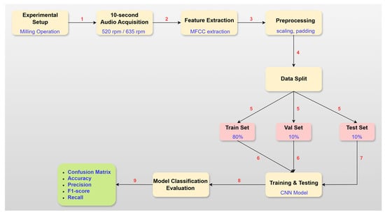
Figure 1. Algorithmic flowchart of the tool-wear classification methodology.

Each speed corresponds to a separate experimental dataset and was used independently for the model training and validation to evaluate the model’s performance. Table 1 summarizes the number of audio recordings of 744 unique physical cutting passes for each tool wear condition at both speeds. For each speed, the dataset is categorized into four different tool wear conditions following ISO 3685 tool-life testing standard definitions:

-

Condition 1_Idle: Machine running without any cutting operations.

-

Condition 2_Fresh tool: Cutting operation performed using a fresh cutting tool with 0 flank wear.

-

Condition 3_Moderate tool: Cutting operation performed using a moderately worn tool (VB = 0.1–0.2 mm).

-

Condition 4_Worn tool: Cutting operation performed using a worn tool (VB > 0.3 mm).

Table 1. Summary of the audio dataset for the cutting speeds of 520 rpm and 635 rpm.

Condition	520 rpm	635 rpm	Total	Duration (s)
Idle	175	172	347	10
Fresh tool	200	181	381	10
Moderate tool	188	188	376	10
Worn tool	181	203	384	10
Total	744	744	1488	4.13 h

Table 1. Summary of the audio dataset for the cutting speeds of 520 rpm and 635 rpm.

Condition	520 rpm	635 rpm	Total	Duration (s)
Idle	175	172	347	10
Fresh tool	200	181	381	10
Moderate tool	188	188	376	10
Worn tool	181	203	384	10
Total	744	744	1488	4.13 h

2.1. Preprocessing and Feature Extraction

The primary purpose of this study is to classify the tool wear conditions based on acoustic signal of machining operation through a deep learning approach, specifically, Convolutional Neural Network (CNN). However, due to the high dimensionality, temporal dependencies and redundancy in these audio signals, a transformation into a more representative format is necessary for an efficient processing of the data by developed Convolutional Neural Network model to achieve efficient classification. Audible sound signals collected from the sensor are at a high sampling frequency, and the raw dataset is relatively large; therefore, it is not practical to use this data directly as input to the model to monitor the tool wear. Consequently, it is necessary to preprocess raw data and extract useful features that indicate relation to tool wear. To address this, at the preprocessing stage Mel-Frequency Cepstral Coefficients (MFCCs), which represent the short-term power spectrum of a sound based on human auditory perception [21], were extracted from each recording to construct suitable input representations. MFCCs are widely used features that have been successfully implemented not only in sound signal processing [22] but also in various machine-condition and machining-related acoustic monitoring tasks [8,11]. The MFCCs were computed through the steps, including framing, windowing, Discrete Fourier Transformation (DFT), Mel Filter Bank processing, logarithmic scaling and finally Discrete Cosine Transform (DCT), resulting in a set of cepstral coefficients that represent the essential features of the audio signals [23]. At the initial framing and windowing step, the complex and big raw data signal was split into frames with stationary signal, which allows stable acoustic characterization. Later, each frame power spectrum, which is the distribution of the power of the frequency components that compose the signal, was calculated using Discrete Fourier Transform as in Equation (1) [24], where $x\left(n\right)$ is discrete signal, and $N$ is the length of the signal.

$$X\left(k\right)=\sum _{n=0}^{N-1}x(n)e^{-{\displaystyle \frac{2\pi jnK}{N}}} k=1,2,3,\dots ,N-1$$

(1)

The filtering of the signal was performed using Mel band-pass filter, which targets extracting non-linear representation of the audible sound signal. Finally, a Discrete Cosine Transform was used for summation of cosine functions oscillating at different frequencies. Here, Discrete Cosine Transform was applied to the Mel filter bank to select most accelerative coefficients or to separate the relationship in the log spectral magnitudes from the filter-bank [25], using Equation (2).

$$X\left(k\right)=\sum _{n=0}^{N-1}x\left(n\right)\ast Cos\left({\displaystyle \frac{2\pi jnK}{N}}\right) k=1,2,3,\dots ,N-1$$

(2)

In the process of analyzing audible sound signals of machining operations, MFCCs were extracted using the Librosa library in Python (version 3.9.23), which performed all steps mentioned above.

The audio dataset described in Table 1 contains recordings of machining operations, each 10 s long, recorded with 48 kHz sampling rate. Therefore, each audio signal has 480,000 total number of samples, calculated as the multiplication of the sampling rate (48 kHz) and the duration of recording (10 s). Each recording was divided into overlapping frames of 25 ms duration, which falls within the recommended range of 20–30 ms for short-term spectral analysis in acoustic signals [23]. The number of samples in each frame is therefore 1200. A sliding window with a duration of 10 ms, corresponding to 480 samples at the 48 kHz sampling rate, was applied between consecutive frames. This shift was sufficient to capture gradual temporal changes in such signals [23]. As a result of this windowing, approximately 998 overlapping frames were constructed for each 10 s recording. To ensure consistent input length across all recordings, zero-padding was applied to set each recording to a fixed frame length of 1000. In this study, 13 MFCCs were extracted to construct the size of 13 × 1000 time-frequency representations for each 10 s recording as adopted in the literature [26,27]. Defining an appropriate number of MFCCs plays crucial role in capturing the essential spectral features of the acoustic signals [28]. Lower order MFCCs (typically first 12–13) capture the dominant spectral envelope and energy distribution of the signal, while higher order coefficients mainly encode rapid and noise detailed spectral fluctuations, which enable non-informative components in the feature space and reduce model’s classification performance [23,28,29]. Hasan et al. [28] demonstrated this effect experimentally by comparing the MFCC sets of 12, 24, 40 and 60 coefficients and concluded that performance decreased as the number of coefficients increased, confirming that 12 MFCCs provided the best classification performance. Figure 2 illustrates the heatmaps of one of the recordings at 635 rpm extracted from each tool wear condition provided in Table 1. Each heatmap consists of 13 MFCCs for the 10 s recording. The first two MFCCs, shown in blue and red, represent the overall energy and the spectral shape of the recordings, and remain stable across all conditions. In MFCC plots the color scale units are in decibels (dB), where red values represent higher log-energy in specific frequency band, and blue values represent lower log-energy. However, unlike an amplitude in sound pressure level described by decibels, MFCC values do not have direct physical meaning; what is more important here is the relative difference between selected classes. It is clear to observe that the Idle condition, which represents sound of vertical milling machine, shows minimal variation across all coefficients in the acoustic signal, indicating that no cutting operation exists. The heatmap of the Fresh Tool condition exhibits larger variations and more organized patterns across the coefficients compared to the Idle condition, indicating the presence of a cutting operation with a sharp tool. The heatmap of Moderate Worn Tool condition shows reduction in variations and contrast, caused by irregularities introduced by a slightly worn tool. Finally, in case of machining with worn, the variations seem more disorganized and with lower contrast levels compared to the other conditions. 10 s recording of each tool wear condition was transformed through MFCC extraction into a matrix form with the size of (13, 1000), where 13 represents the number of cepstral coefficients and 1000 the number of time frames. These are the inputs that were applied along with their categorical labels into a Convolutional Neural Network, designed to effectively classify the data into four different categories: Idle, Fresh, Moderate and Worn tool. In addition, to improve the model’s efficiency, each input was individually scaled using the Standard Scaler, which transforms each feature to follow a mean of 1 and variance of 0. For both 520 rpm and 635 rpm, the corresponding audio data was split into training set (80%), validation set (10%) and test set (10%) separately. In total, 595 recordings were used for training set, 74 recordings for validation set, and 75 recordings for the test set, which were unseen by the model and used for evaluating the model performance.

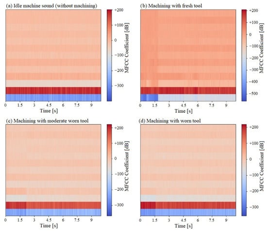
Figure 2. MFCC heatmaps (13 coefficients) of one 10 s audio recording from each tool wear condition at 635 rpm.

2.2. Convolutional Neural Network (CNN)

Convolutional Neural Network (CNN) is a type of deep learning algorithm that learns hierarchical feature representations through convolutional, pooling and fully connected layers and is widely used in classification tasks [30]. CNNs provide strong performance in various domains, such as image recognition [31], speech processing [32] and acoustic signal classification [33]. The use of CNNs has demonstrated high accuracy in detecting tool wear during milling of gears [11]. In this study, the Mel-Frequency Cepstral Coefficients (MFCCs) features obtained from tool cutting operations were structured as two-dimensional matrices, enabling the CNN to learn the discriminative features for tool wear classification, where local features were extracted by the convolutional layers, dimensionality reduction was performed by the pooling layers and final classification was carried out by the fully connected layers. The architecture of the designed CNN used for tool wear classification from the MFCC representations of milling acoustic signals is illustrated in Figure 3.

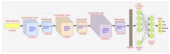
Figure 3. CNN architecture for classifying tool wear conditions using MFCC representations of milling acoustic signals.

The input to the model is a 13 × 1000 × 1 tensor where 13 represents the MFCCs, and 1000 represents the time frame. Each convolutional layer uses a 3 × 3 kernel with stride 1. The first convolutional block applies 32 filters with ReLU activation and produces a 13 × 1000 × 32 feature map, which is then reduced to 13 × 500 × 32 through a 1 × 2 max-pooling layer with stride 2. The second block applies 64 ReLU filters, generating a 13 × 500 × 64 representation that is further reduced to 13 × 250 × 64 by max-pooling. The third block applies 128 filters with ReLU activation, producing a 13 × 250 × 128 feature map that is down-sampled to 13 × 125 × 128. After the final max-pooling operation, the resulting 13 × 125 × 128 feature maps are flattened into a single vector, which is then passed through a fully connected layer with 128 ReLU activation units and a 0.3 dropout rate, followed by a final Softmax layer with 4 neurons that outputs the probabilities (p₁, p₂, p₃, p₄) for the four tool-wear classes: Idle, Fresh, Moderate and Worn. The model was trained and evaluated on a system with 11th Gen Intel Core i7-1165G7 processor (2.80 GHz), 16 GB RAM, and a 64-bit operating system. The training hyperparameters used in this study are shown in Table 2.

Table 2. Training hyperparameters for the designed CNN model.

Hyper Parameter	Value
Optimizer	Adam
Learning rate	0.0001
Loss function	Categorical cross-entropy
Epoch	30
Batch Size	16
Early Stopping patience	5
Train/Val/Test Split	80%/10%/10%
Scaler	Standard Scaler
Evaluation metric	Accuracy

3. Results and Discussion

The CNN model was trained separately on the extracted MFCC inputs for both datasets with cutting speeds of 520 rpm and 635 rpm. Figure 4 presents the training and validation loss and accuracy curves for both datasets. In both cases, training loss and validation loss decreased rapidly during the first 10–12 epochs and then began to stabilize, indicating that the model converged. Similarly, the accuracy increased during this period and stabilized at above 0.9. The validation curves for both datasets closely followed the training curves, indicating strong generalization and negligible overfitting.

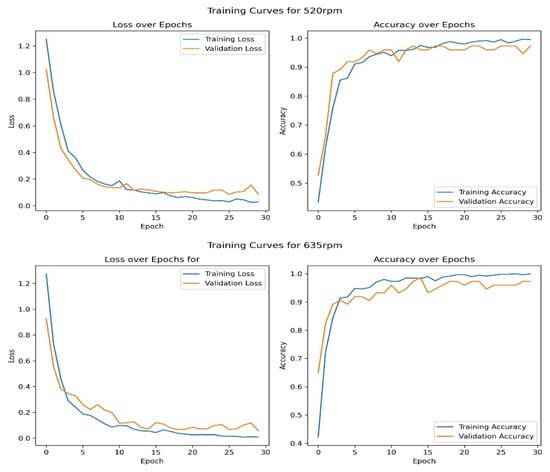
Figure 4. Training vs. Validation Loss and accuracy curves for both 520 rpm and 635 rpm datasets.

To further evaluate the performance of the model, the unseen test sets from both 520 rpm and 635 rpm datasets were evaluated using their separately trained CNN models. The model trained on the 635 rpm dataset achieved an accuracy of 98.67% on its corresponding test set, while the model trained on the 520 rpm dataset achieved an accuracy of 94.67% on its corresponding test set. To assess the stability of the proposed model and reduce the impact of algorithmic randomness, the training was repeated three times for both speeds. For the 520 rpm dataset, the validation accuracies across the three runs were 98.65%, 97.3% and 94.59%, giving an average accuracy of 96.85 ± 2.07%. For the 635 rpm dataset, the runs yielded 95.95%, 93.24% and 91.89% accuracies with an average of 93.69 ± 2.07%. These small variations show that the model is stable and not sensitive to random initialization.

The performance metrics of each class for both datasets at cutting speeds of 520 rpm and 635 rpm were summarized in Table 3, using the widely adopted metrics of precision, recall and F1-score, and the corresponding confusion matrices are presented in Figure 5. Precision measures the correctness of predictions for a class, and recall indicates the proportion of actual samples of that class that are correctly identified. F1-score is the combination of precision and recall, showing the balance between them [34]. At 520 rpm, most misclassifications occurred between Fresh and Moderate tools. One Idle tool sample was misclassified as Fresh, one Fresh tool as Moderate and two Moderate tools as Fresh. Consequently, the Fresh tool had the lowest precision of 0.86, and the Moderate tool showed lowest recall of 0.89. On the other hand, Worn tools were successfully classified with no errors. At 635 rpm, it is clear to observe the improvement in classification. Idle, Moderate and Worn tools achieved perfect precision, recall and F1-score. The only misclassification that occurred at 635 rpm was between the Fresh tool and Moderate tool, where one Fresh tool sample was predicted as Moderate, and this caused a recall value of 0.94. These results demonstrate that the developed hybrid model with Mel-Frequency Cepstral Coefficients (MFCCs), used for feature extraction from audible sound, and Convolutional Neural Network (CNN), used for classification of the tool wear conditions, can successfully identify the Idle working condition of the milling center and Worn tool classes due to their different acoustic features.

Table 3. Classification performance of the CNN for tool wear conditions at 520 rpm and 635 rpm.

	520 rpm			635 rpm
	Precision	Recall	F1-Score	Precision	Recall	F1-Score
Idle	1.00	0.94	0.97	1.00	1.00	1.00
Fresh	0.86	0.95	0.90	1.00	0.94	0.97
Moderate	0.94	0.89	0.92	0.95	1.00	0.97
Worn	1.00	1.00	1.00	1.00	1.00	1.00

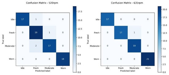
Figure 5. Confusion matrices for both 520 rpm and 635 rpm.

4. Conclusions and Future Work

Due to the demands of intelligent manufacturing, the timely detection of tool wear conditions is essential to improve the production quality, increase productivity, optimize maintenance costs, and minimize the manufacturing losses. Various monitoring systems employing different types of sensing techniques have been presented in the literature to detect the tool conditions and to recognize premature tool failure. In this paper, a hybrid technique that employs Mel-Frequency Cepstral Coefficients (MFCCs) for feature extraction from an audible sound and a Convolutional Neural Network (CNN) deep learning algorithm for classification of the tool wear conditions was used to analyze machining sound signals collected during the milling of the mild steel workpiece with cutting tools at different wear stages. The experimental results revealed clear characteristic components in the milling sound signal related to the tool wear. Testing and classification results have demonstrated that the developed hybrid model can easily differentiate between the Idle working condition of the milling center and Worn tool classes; accuracies across the three runs at 520 rpm were 98.65%, 97.3% and 94.59%, giving an average accuracy of 96.85 ± 2.07%, and, for the 635 rpm dataset, the runs yielded 95.95%, 93.24% and 91.89% accuracies with an average of 93.69 ± 2.07%. The CNN model was preferred in this study because MFCCs provide a structured time–frequency representation where wear-related patterns appear as local spectral variations. CNNs learn such localized patterns efficiently and are computationally lightweight, making them suitable for real-time monitoring. In contrast, other deep learning architectures, such as GRUs, LSTMs and Transformers are designed for long raw sequences and require much larger datasets and computational resources.

While the current study demonstrates the feasibility of using acoustic signals and a CNN-based model for tool wear classification, several directions can enhance both generalizability and industrial applicability. It should be noted that the present experimental study is limited to a single workpiece material and a narrow range of cutting speeds, which may restrict the direct generalization of the obtained results to other machining conditions. Future work may focus on expanding the experimental conditions to include multiple workpiece materials, tool geometries, cutting parameters, enabling the model to generalize across a broader range of machining scenarios. Such extensions will allow a more systematic evaluation of model robustness and transferability across different operating regimes. Additionally, to further improve robustness under varying machining conditions, adaptive deep-learning and attention-based mechanisms may be explored in future work. Integrating hybrid or sequential deep-learning architectures and multi-sensor data fusion could better capture temporal dependencies and complex process dynamics. Finally, advanced noise reduction and signal enhancement techniques may be explored to improve model robustness under realistic industrial environments.

References

- Li, G.; Shang, X.; Sun, L.; Fu, B.; Yang, L.; Zhou, H. Application of audible sound signals in tool wear monitoring: A review. Adv. Manuf. Sci. Technol. 2025, 5, 2025003. [Google Scholar] [CrossRef]
- Mamedov, A.; Dinc, A.; Guler, M.A.; Demiral, M.; Otkur, M. Tool wear in micromilling: A review. Int. J. Adv. Manuf. Technol. 2025, 137, 47–65. [Google Scholar] [CrossRef]
- Pimenov, D.Y.; Kumar Gupta, M.; da Silva, L.R.; Kiran, M.; Khanna, N.; Krolczyk, G.M. Application of measurement systems in tool condition monitoring of Milling: A review of measurement science approach. Measurement 2022, 199, 111503. [Google Scholar] [CrossRef]
- Gururaja, S.; Singh, K.K. Development of smart manufacturing framework for micromilling of thin-walled Ti6Al4V. Mach. Sci. Technol. 2024, 28, 459–488. [Google Scholar] [CrossRef]
- Abhilash, P.M.; Chakradhar, D. Performance monitoring and failure prediction system for wire electric discharge machining process through multiple sensor signals. Mach. Sci. Technol. 2022, 26, 245–275. [Google Scholar] [CrossRef]
- Wegener, K.; Bleicher, F.; Heisel, U.; Hoffmeister, H.-W.; Möhring, H.-C. Noise and vibrations in machine tools. CIRP Ann. 2021, 70, 611–633. [Google Scholar] [CrossRef]
- Unal, P.; Deveci, B.U.; Ozbayoğlu, A.M. A Review: Sensors Used in Tool Wear Monitoring and Prediction. In Lecture Notes in Computer Science; Springer: Cham, Switzerland, 2022; Volume 13475. [Google Scholar] [CrossRef]
- Li, Z.; Liu, R.; Wu, D. Data-driven smart manufacturing: Tool wear monitoring with audio signals and machine learning. J. Manuf. Process. 2019, 48, 66–76. [Google Scholar] [CrossRef]
- Zafar, T.; Kamal, K.; Mathavan, S.; Hussain, G.; Alkahtani, M.; Alqahtani, F.M.; Aboudaif, M.K. A Hybrid Approach for Noise Reduction in Acoustic Signal of Machining Process Using Neural Networks and ARMA Model. Sensors 2021, 21, 8023. [Google Scholar] [CrossRef]
- Ai, C.S.; Sun, Y.J.; He, G.W.; Ze, X.B.; Li, W.; Mao, K. The milling tool wear monitoring using the acoustic spectrum. Int. J. Adv. Manuf. Technol. 2012, 61, 457–463. [Google Scholar] [CrossRef]
- Kanakasuntharam, J.; Wijethunge, A. CNN and ANN Based Tool Condition Monitoring in Gear Machining Using Audio and Vibration Signals Via Cost Effective Sensors. In Proceedings of the International Conference on Emerging Smart Computing and Informatics (ESCI), Pune, India, 5–7 March 2024; pp. 1–6. [Google Scholar] [CrossRef]
- Liu, M.K.; Tseng, Y.H.; Tran, M.Q. Tool wear monitoring and prediction based on sound signal. Int. J. Adv. Manuf. Technol. 2019, 103, 3361–3373. [Google Scholar] [CrossRef]
- Peng, C.-Y.; Raihany, U.; Kuo, S.-W.; Chen, Y.-Z. Sound Detection Monitoring Tool in CNC Milling Sounds by K-Means Clustering Algorithm. Sensors 2021, 21, 4288. [Google Scholar] [CrossRef]
- Han, S.; Mannan, N.; Stein, D.C.; Pattipati, K.R.; Bollas, G.M. Classification and regression models of audio and vibration signals for machine state monitoring in precision machining systems. J. Manuf. Syst. 2021, 61, 45–53. [Google Scholar] [CrossRef]
- Ntalampiras, S. One-shot learning for acoustic diagnosis of industrial machines. Expert Syst. Appl. 2021, 178, 114984. [Google Scholar] [CrossRef]
- Zhou, Y.; Sun, B.; Sun, W.; Lei, Z. Tool wear condition monitoring based on a two-layer angle kernel extreme learning machine using sound sensor for milling process. J. Intell. Manuf. 2022, 33, 247–258. [Google Scholar] [CrossRef]
- Liu, T.H.; Chi, J.Z.; Wu, B.L.; Chen, Y.S.; Huang, C.H.; Chu, Y.S. Design and Implementation of Machine Tool Life Inspection System Based on Sound Sensing. Sensors 2023, 23, 284. [Google Scholar] [CrossRef] [PubMed]
- Wu, M.; Yao, Z.; Verbeke, M.; Karsmakers, P.; Gorissen, B.; Reynaerts, B. Data-driven models with physical interpretability for real-time cavity profile prediction in electrochemical machining processes. Eng. Appl. Artif. Intell. 2025, 160, 111807. [Google Scholar] [CrossRef]
- Yao, Z.; Wu, M.; Qian, J.; Reynaerts, D. Intelligent discharge state detection in micro-EDM process with cost-effective radio frequency (RF) radiation: Integrating machine learning and interpretable AI. Expert Syst. Appl. 2025, 291, 128607. [Google Scholar] [CrossRef]
- Soni, N.; Kumar, A.; Patel, H. Acoustic Analysis of Cutting Tool Vibrations of Machines for Anomaly Detection and Predictive Maintenance. In Proceedings of the IEEE 11th Region 10 Humanitarian Technology Conference (R10-HTC), Rajkot, India, 16–18 October 2023; pp. 43–46. [Google Scholar] [CrossRef]
- Kumar, A.; Yadav, J. Machine learning for audio processing: From feature extraction to model selection. Mach. Learn. Models Archit. Biomed. Signal Process. 2025, 97–123. [Google Scholar] [CrossRef]
- Liang, B.; Iwnicki, S.D.; Zhao, Y. Application of power spectrum, cepstrum, higher order spectrum and neural network analyses for induction motor fault diagnosis. Mech. Syst. Signal Process. 2013, 39, 342–360. [Google Scholar] [CrossRef]
- Abdul, Z.K.; Al-Talabani, A.K. Mel Frequency Cepstral Coefficient and its Applications: A Review. IEEE Access 2022, 10, 122136–122158. [Google Scholar] [CrossRef]
- Feldman, H.A.; Kaiser, N.; Peacock, J.A. Power-spectrum analysis of three-dimensional redshift surveys. Astrophys. J. 1994, 426, 23. [Google Scholar] [CrossRef]
- Strang, G. The discrete cosine transform. SIAM Rev. 1999, 41, 135–147. [Google Scholar] [CrossRef]
- Yang, X.; Yu, H.; Jia, L. Speech Recognition of Command Words Based on Convolutional Neural Network. In Proceedings of the International Conference on Computer Information and Big Data Applications, Guiyang, China, 17–19 April 2020; pp. 465–469. [Google Scholar] [CrossRef]
- Wahyuni, E.S. Arabic speech recognition using MFCC feature extraction and ANN classification. In Proceedings of the 2nd International Conferences on Information Technology, Information Systems and Electrical Engineering, Yogyakarta, Indonesia, 1–3 November 2017; pp. 22–25. [Google Scholar] [CrossRef]
- Hasan, R.; Hasan, M.; Hossein, Z. How many Mel-frequency cepstral coefficients to be utilized in speech recognition? A study with the Bengali language. J. Eng. 2021, 12, 817–827. [Google Scholar] [CrossRef]
- O’Shaugynessy, D. Speech Communications: Human and Machine; Wiley-IEEE Press: Hoboken, NJ, USA, 2000; ISBN 978-0-780-33449-6. [Google Scholar]
- Rawat, W.; Wang, Z. Deep Convolutional Neural Networks for Image Classification: A Comprehensive Review. Neural Comput. 2017, 29, 2352–2449. [Google Scholar] [CrossRef]
- Krizhevsky, A.; Sutskever, I.; Hinton, G.E. ImageNet classification with deep convolutional neural networks. Adv. Neural Inf. Process. Syst. 2012, 25, 1097–1105. [Google Scholar] [CrossRef]
- Abdel-Hamid, O.; Mohamed, A.R.; Jiang, H.; Deng, L.; Penn, G.; Yu, D. Convolutional neural networks for speech recognition. IEEE/ACM Trans. Audio Speech Lang. Process. 2014, 22, 1533–1545. [Google Scholar] [CrossRef]
- Piczak, K.J. Environmental sound classification with convolutional neural networks. In Proceedings of the IEEE 25th International Workshop on Machine Learning for Signal Processing, Boston, MA, USA, 17–20 September 2015; pp. 1–6. [Google Scholar] [CrossRef]
- Sokolova, M.; Lapalme, G. A systematic analysis of performance measures for classification tasks. Inf. Process. Manag. 2009, 45, 427–437. [Google Scholar] [CrossRef]
Disclaimer/Publisher’s Note: The statements, opinions and data contained in all publications are solely those of the individual author(s) and contributor(s) and not of MDPI and/or the editor(s). MDPI and/or the editor(s) disclaim responsibility for any injury to people or property resulting from any ideas, methods, instructions or products referred to in the content. |
© 2026 by the authors. Licensee MDPI, Basel, Switzerland. This article is an open access article distributed under the terms and conditions of the Creative Commons Attribution (CC BY) license.