Abstract
The adaptability of a hexapod robot to complex terrain is highly dependent on its own posture, which directly affects its stability and flexibility. In order to adapt to a change in terrain, it is necessary to adjust posture in real time when walking. At the same time, external factors such as ground state and landing impact will also interfere with posture. Therefore, it is necessary to maintain balance after adjustment. This paper proposes a pose adjustment method utilizing joint angle control. It enhances robot stability, flexibility, and terrain adaptability through torso posture and center of gravity optimization, aiming to maintain balance. The strategy’s effectiveness was validated via Adams–Simulink co-simulation. Optimal position and posture adjustment for the torso was then implemented at the six-legged support stage after each step, employing inverse kinematics and a triangular gait. It is found that without pose adjustment, the direction deviation will accumulate and significantly deviate from the trajectory. The introduction of this adjustment can effectively correct the direction deviation and torso posture angle, increase the stability margin, ensure stable straight-line walking, and significantly reduce joint energy consumption. Crawling experiments with the physical prototype further validate the strategy. It rapidly counters instantaneous attitude fluctuations during leg alternation, maintaining a high stability margin and improving locomotion efficiency. Consequently, the robot achieves enhanced directional stability, overall stability, and energy efficiency when traversing terrain.
1. Introduction
As robot technology expands into unstructured environments, the ability to move autonomously in complex terrains has become a core bottleneck restricting intelligent operations. Traditional wheeled or tracked robots, constrained by poor terrain adaptability and limited obstacle-crossing capabilities, are ill-suited for the heavy-load, highly dynamic tasks of mountain rescue, interstellar exploration, and military transport. In contrast, hexapod robots capitalize on multiple degrees of freedom, kinematic redundancy, and discrete footholds to achieve superior rugged terrain adaptation. Their ability to actively adjust posture under load for stable motion positions them as key unmanned carriers in complex environments. However, the coupling effect between overload and complex terrain leads to highly nonlinear robot dynamics, and the uncertainty of foot–ground interaction increases dramatically. How to achieve real-time and robust pose adjustment control is still a difficult point in current research.
In recent years, significant progress has been made in the field of robot control. During 2025, Yuanchun Li et al. [1] completed research on the gait coordination control of bipedal modular reconfigurable robots and proposed a control method based on adaptive neural networks, which effectively reduces position tracking errors and control torque. Norihisa Namura and Hiroya Nakao [2] proposed a central pattern generator (CPG) network for the gait transition of hexapod robots based on phase reduction. By simplifying the dynamic model of the CPG network, the smooth transition of hexapod robots between different typical gaits was achieved. Dong Zhao et al. [3] conducted modeling and stability control research on the steering and deformation motion of a wheel–leg deformation robot, established a dynamic model, designed control strategies, and verified its stability during the steering and deformation process through simulation and experiments. Ahmad M. El Nagar et al. [4] proposed an embedded fuzzy PD controller for robot manipulator arms. By combining a two-degree-of-freedom structure and a fuzzy PD structure, the system uncertainty was effectively reduced. Based on the small gain theorem, the bounded input–output (BIBO) stability of the system was analyzed. The experimental results showed that the controller significantly reduced errors in trajectory tracking and anti-interference tasks. Moharam Habibnejad Korayem et al. [5] proposed a hybrid stable adaptive control method for the navigation of nonholonomic wheeled mobile robots on sliding surfaces. The method combines stable model predictive control (SMPC) and adaptive sliding mode control (ASMC), achieving zero steady-state error, fast error convergence, reliable obstacle avoidance, and robustness to continuous disturbances and uncertainties. Hongsheng Sha et al. [6] proposed a collaborative adaptive consensus tracking control method for multi-wheeled mobile robot systems. This method effectively improves the robustness of the system under model uncertainty and external disturbances by combining a dynamic sliding mode tracker with an uncertainty and disturbance estimator (UDE) and a radial basis function neural network (RBF NN), and its effectiveness is verified through simulation. Kang Xu et al. [7] proposed a horizon stability control method for wheeled–legged robots traveling on unknown and complex terrains. By optimizing the control strategy, the stability and adaptability of a robot traveling on complex terrains were effectively improved. Alessia Li Noce et al. [8] proposed a stable and safe control method for quadruped robot leg balance based on a neural network controller. The neural network was trained through an imitation learning strategy to mimic the behavior of the optimal controller, and stability and safety were ensured using the Lyapunov method and a linear matrix inequality (LMI) framework. Significant progress has been made in the field of robot control, including gait coordination, gait transition, stability control, manipulator arm control, sliding surface navigation, multi-wheeled mobile robot systems, complex terrain driving, and quadruped robot balance control, which have improved the stability, adaptability, and robustness of robots.
With the development of control technology, intelligent robots have become a hotspot in the field of automatic control. Jumpei Yamasaki et al. [9] analyzed the gait and transportation costs of quadruped robots, and studied a quadruped robot based on neural-morphology-integrated circuits, which aim to optimize its motion efficiency and energy consumption. Shanshan Li et al. [10] conducted research on the gait generation and transformation of a (2UPS-U) + R series parallel wheel–leg hybrid quadruped robot. By establishing a dynamic model and control strategy, the robot achieved smooth transitions between different gaits. Yifan Pan et al. [11] proposed a gait and simulation analysis method for quadruped crawling robots based on deformable structures. The robot has enhanced its crawling ability and adaptability in complex environments through deformation mechanisms, and the feasibility and stability of its walking and turning strategies have been verified through virtual prototyping technology. Zhiyong Jiang et al. [12] studied the motion planning and control problem of humanoid robots under environmental uncertainty, and proposed an effective control strategy to improve the motion stability and adaptability of robots in complex environments. Moh ShahidKhan et al. [13] proposed an optimized PID control method for the stability of a 16-degree-of-freedom bipedal robot when crossing ditches. By adjusting the control parameters, the stability and obstacle-crossing ability of the robot on complex terrains were significantly improved. Tingting Guo et al. [14] proposed an innovative active disturbance motion control method for an underwater adsorption climbing robot with uncertainty and compensation. This method effectively improves the motion accuracy and stability of the robot in complex underwater environments. Lin Yu et al. [15] proposed an iterative learning-based tracking control method for two-wheeled mobile robots, which can effectively handle model uncertainty and unknown periodic disturbances. This method significantly improves the tracking accuracy and stability of robots in complex environments. Hao Cheng and Xuejun Wang [16] studied the stability control strategy of an adjustable-pressure wall-climbing robot based on adsorption recognition. By establishing an adsorption force model and designing an adaptive controller, the robot’s adsorption stability and crawling performance were improved under different wall conditions. Ming Han et al. [17] studied the problem of time–energy optimal trajectory planning for articulated heavy-duty robots and proposed a trajectory planning method based on time and energy optimization. By optimizing the control strategy, the robot achieved efficient motion in complex tasks. Research in robot control spans diverse areas, including quadrupedal gait optimization, gait transition strategies for parallel-legged robots, terrain adaptability enhancement in crawling robots, stability augmentation for humanoid locomotion, obstacle-crossing capability breakthroughs in bipedal systems, motion precision refinement of underwater robots, tracking accuracy improvements for wheeled balancing platforms, and adhesion stability control in wall-climbing mechanisms. These advancements collectively elevate robotic performance and operational efficiency in complex environments.
In the field of attitude control, He Zhu et al. [18] designed a fuzzy gait control algorithm for multi-legged hydraulic robots, which achieved autonomous navigation closed-loop control through fuzzy neural networks (FNNs). The algorithm solved the shaking and impact problems under traditional algorithm control and successfully achieved rotational gait motion. Song Dongfang et al. [19] studied the attitude stability control system of a mobile robot mechanism based on nanosensors, but the specific control strategy and experimental results were not mentioned in the search results. Kang Xu et al. [20] proposed a whole-body stability control method for a wheeled–legged hexapod robot on complex terrain, which combines event-triggered interference control and whole-body stability control to effectively improve the stability of the robot on complex terrain. Yanchao Sun et al. [21] proposed an adaptive interval type-2 fuzzy control method for multi-legged underwater robots, which solves the problem of input saturation full-state constraints and improves the robot’s motion performance in complex environments. Lixia Fang et al. [22] proposed a coordinated and consistent optimal control method for underground heavy-duty robots in unstructured environments, which improves the motion efficiency and stability of the robot in complex environments. Researchers have made progress in the gait control of multi-legged hydraulic robots, posture stability of mobile robots, full body stability of wheeled–legged hexapod robots, adaptive control of multi-legged underwater robots, and coordinated consistency control of underground heavy-duty robots. Through technologies such as fuzzy neural networks, event-triggered control, and adaptive control, the motion performance and stability of robots in complex environments have been improved.
During the year 2022, Yalong Yang et al. [23] conducted research on the gait simulation of a two-degree-of-freedom lower limb rehabilitation robot based on ADAMS 2018 and MATLAB 2018. Through dynamic modeling and simulation analysis, the motion performance of the rehabilitation robot under different gait modes was verified. Shunxiang Wei et al. [24] proposed a gait planning and motion performance analysis method for quadruped robots based on a central pattern generator (CPG) and backpropagation neural network (BPNN). By optimizing the duty cycle of walking gait, gait planning and smooth switching were achieved. Fakang Liao et al. [25] studied the gait transition and trajectory stability analysis of a bipedal robot based on the V-DSLIP model, proposed a gait transition strategy, achieved walking gait transition by controlling leg stiffness and hip torque, and analyzed the trajectory stability of the bipedal robot system using the Poincaré mapping method. Ito Kazuyuki et al. [26] studied a multi-legged robot, URARAKA VI, with suction cups for climbing walls and pipelines. Through structural design and motion control, the robot’s climbing ability and stability on complex surfaces were improved. Yuanxi Sun et al. [27] proposed a novel involute arc-shaped leg structure for multi-legged robots, which has the characteristics of high stability and low energy consumption. Its motion performance on complex terrains was verified through kinematic analysis and simulation. These studies have improved the motion performance and stability of robots in different application scenarios through methods such as dynamic modeling, neural network optimization, gait transition strategies, motion control, and kinematic analysis.
In addition, Mahkam Nima and Özcan Onur [28] analyzed the gait and motion of a soft hybrid multi-legged modular micro-robot and studied its motion performance on different terrains. Ozkan Aydin Yasemin et al. [29] studied how a self-reconfigurable multi-legged robot cluster can work together to complete challenging terrain dynamics tasks. Muñoz Filiberto et al. [30] proposed an adaptive tracking control method based on dynamic neural networks for autonomous underwater vehicles affected by modeling and parameter uncertainties. Mohammad Reza Soltanpour et al. [31] proposed a free flutter fuzzy sliding mode control method for joint flexible robot manipulators to address matching and mismatch uncertainties in model dynamics and actuators. Yuxiang Wang et al. [32] improved the positioning accuracy of heavy-duty robots by combining model-based geometric parameter recognition and optimizing neural networks to compensate for non-geometric errors. Hanwen Yu et al. [33] conducted frequency response analysis on a heavy-duty palletizing robot by considering elastic deformation. Zeming Long et al. [34] proposed a control strategy for a hydraulic hybrid servo drive system for heavy-duty robots. Bo You et al. [35] studied the low-speed control of a long-telescopic-arm heavy-duty handling robot based on the Stribeck friction model. These studies enhance the motion performance and control accuracy of robots in diverse terrains and complex tasks through techniques such as gait analysis, cluster collaboration, adaptive tracking control, fuzzy sliding mode control, geometric parameter recognition, frequency response analysis, and servo drive system control.
A pose adjustment control framework for hexapod heavy-duty robots is proposed to maintain stable motion through pose adjustment. Firstly, adjust the center of gravity of the quadruped robot to the maximum stability margin using zero moment points to maintain the stability of the robot’s center of gravity. Secondly, pose adjustment requires finding the optimal pose for a flat hexapod robot between flexibility and stability, achieving the coordinated optimization of movement conditions and body pose under heavy load conditions. Finally, a physical prototype of the hexapod robot and a multi-terrain simulation platform were built to verify the effectiveness of the proposed method in sloping and irregular scenes. The specific research content and chapter arrangement are as follows: The introduction introduces the research background and significance of the topic, and outlines the current application requirements of hexapod robots in complex terrain. This article elaborates on the research status and related applications of hexapod robots in complex terrains both domestically and internationally. The first section introduces the robot pose adjustment scheme. The second section introduces the analysis of pose adjustment methods for hexapod robots. The third section mainly introduces the experimental simulation and physical verification of the pose adjustment of hexapod robots, and completes the analysis of the experimental results. The fourth section is the conclusion of the entire text.
1.1. Robot Pose Adjustment Method
The stability and flexibility of hexapod robots are contradictory, so pose adjustment needs to be balanced between the stability and flexibility of a robot. When a robot has a large number of supporting feet and the ground is relatively flat, the stability of the robot is high. Optimal pose adjustment can be used to improve the maneuverability of a robot while ensuring a sufficient stability margin. When a robot has fewer supporting feet and the ground is complex and rugged, the stability margin of the robot sharply decreases. Current research in pose adjustment prioritizes enhancing robot stability through center of gravity optimization and maximizing the stability margin of hexapod platforms. This motivates integrating dynamic center of gravity control into robotic pose regulation systems. The following section details our proposed center-of-gravity-based pose adjustment framework.
1.1.1. Robot Body Posture Adjustment
When a hexapod robot travels on rugged terrain, its torso will rise and fall with the terrain’s undulations. From a stability perspective, it is not conducive to the control of robots. For enhanced rugged terrain traversal, hexapod robots can adopt an optimal terrain adaptation strategy prior to full pose adjustment, aligning the torso plane with the best fit plane defined by supporting footholds while maintaining other pose parameters. This targeted torso–terrain parallelism significantly improves motion stability and maneuverability when navigating irregular surfaces. A structural model of a hexapod robot is shown in Figure 1.
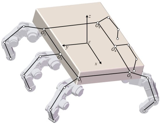
Figure 1.
Structural model of a hexapod robot.
During three-legged gait locomotion in a hexapod robot, let denote the angle between the support tripod’s foothold plane and the horizontal terrain plane. Using forward kinematics, we calculate the torso’s ground-relative pose orientation, , subsequently deriving the value of . Then, during hexapod robot torso posture adjustment, both the foothold positions, , in the global coordinate system and the torso’s centroid location remain invariant, ensuring kinematic consistency throughout the reconfiguration process. The position coordinates of the foot end of a hexapod robot in its torso coordinate system are . Due to the reference pose being fixed to the torso during posture adjustment, the position of the foot end in the torso coordinate system changes with posture adjustment. Figure 2 shows the adjustment of the robot’s body posture. The blue part in the figure represents the pose of the robot before adjustment, and the green part represents the pose of the robot body parallel to the ground after adjustment.
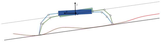
Figure 2.
Robot body posture adjustment.
Use the known position coordinates, , of the foot relative to the geodetic coordinate system and the pose parameters, , of the robot body after adjusting its posture relative to the geodetic coordinate system. At this point, the pose transformation matrix of the aircraft relative to the geodetic coordinate system is as follows:
where is the coordinate of the robot body relative to the pose parameter, , in the geodetic coordinate system, and are the yaw angle, pitch angle, and roll angle, respectively. Taking the body coordinate system as the reference coordinate system, Figure 3 shows the D-H coordinate system of the robot leg. In the figure, represent the joint angle and trunk length, respectively. Multiplying adjacent D-H transformation matrices yields the transformation matrix, , from the foot coordinate system to the base coordinate system, which is as follows:
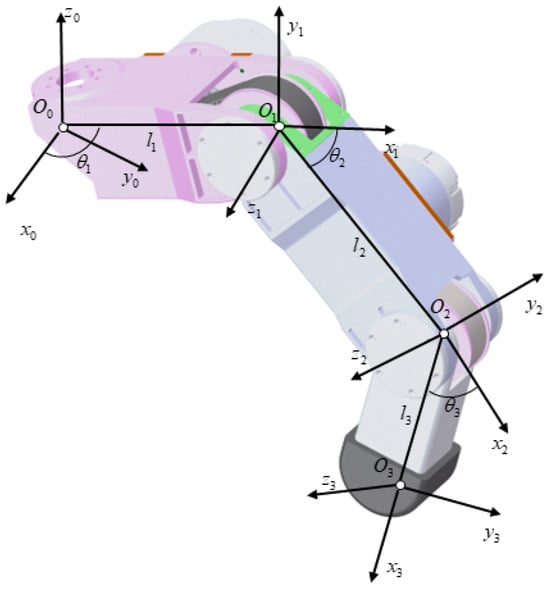
Figure 3.
Robot leg D-H coordinate system.
In the formula, represent the sine and cosine respectively. Thus, based on the known position coordinates, , of the foot relative to the geodetic coordinate system, the pose transformation matrix, , of the body relative to the geodetic coordinate system, and the transformation matrix, , from the end coordinate system to the base coordinate system, obtain the relationship between the position coordinates, , of the foot relative to the earth coordinate system and the corresponding leg joint angle, :
Then obtain the values of the angles, , of each joint of the legs of the hexapod robot. The obtained rotation angle is used for the position control of leg joints, ultimately achieving body posture adjustment of the hexapod robot.
1.1.2. Adjustment of the Robot’s Center of Gravity
During leg swing transitions in hexapod robots, the shifting center of gravity induced by limb motion introduces unwanted dynamic coupling with posture adjustment. To mitigate this interference under tripod support conditions, center of gravity position optimization becomes critical for stability enhancement. Proactive stabilization can be achieved by preemptively relocating the center of gravity to the centroid of the anticipated support polygon formed by the next-step stance legs before swing leg liftoff. This strategic center of gravity migration ensures maximum instantaneous stability margin at swing-phase initiation.
The important feature of a hexapod robot is its adaptability to complex and unstructured terrain, which requires the robot to have high reliability and stability. The static stability margin for a hexapod robot is quantified as the shortest distance from the vertical projection of the robot’s center of mass within the support polygon to the nearest edge of this polygon. The larger the value of the stability margin, the higher the stability, and if a robot’s it may overturn. It indicates that the magnitude of the stability margin is directly related to the center of gravity position of the hexapod robot. Therefore, in order for hexapod robots to achieve stable walking on unstructured terrain, it is necessary to coordinate with the adjustment of the robot’s center of gravity position to improve its walking stability. The larger the stability margin of a hexapod robot, the more stable it is. When designing the gait of the robot, every step of the gait cycle is attempting to maximize its stability margin. Therefore, it is necessary to study the conditions for robots to achieve the maximum stability margin under various support conditions. For hexapod robots operating on flat terrain, all supporting feet remain coplanar within a horizontal support polygon, with the center of gravity inherently contained within this stability boundary. In contrast, traversing unstructured environments (slopes or rough terrain) typically results in non-coplanar footholds, necessitating the projection of both the center of gravity and support points onto a reference horizontal plane to calculate the effective stability margin. As shown in Figure 4, the hexagon on the slope is a projection of the hexapod robot.
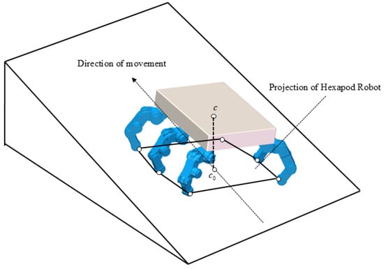
Figure 4.
Projection of hexapod robot on a slope.
The stability margin, , refers to the projection of the center of gravity onto the supporting polygon. Figure 5 shows the centroid projection of the robot within the supporting polygon. In the figure, represents the stability margin of the robot, and represents the stability margin in the direction of motion. The shortest distance from the center of gravity to the supporting polygon edge can be expressed as follows:
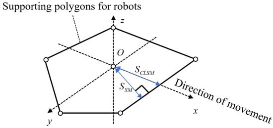
Figure 5.
Projection of the center of mass for supporting polygonal inner robots.
In the formula, represents the vertical distance from the center of gravity to the supporting edge, and represents the coefficient of the supporting edge in the plane coordinate system.
For a hexapod robot in a tripod stance, the stability margin is maximized when the vertical projection of the center of mass coincides with the centroid of the support triangle. Assuming that the coordinates of the three supporting feet at this time are , and the three side lengths of the supporting polygon are , the inner coordinates of the supporting polygon can be obtained as follows:
At this point, it is necessary to adjust the robot’s to in order to obtain the position coordinate, , of the foot relative to the earth coordinate system. During torso center of mass optimization in hexapod robots, both the foothold positions, , defined in the global coordinate frame and the torso’s inertial orientation remain invariant. This kinematic constraint preserves system stability throughout the gravitational compensation process. The position coordinate of the foot end of a hexapod robot in its torso coordinate system is . Due to the fixed connection between the pose and the torso during center of gravity adjustment, the position, , of the foot end in the torso coordinate system changes with the pose adjustment. Similarly, based on the known position coordinates, , of the foot relative to the geodetic coordinate system, the pose transformation matrix A of the body relative to the geodetic coordinate system, and the transformation matrix, , from the end coordinate system to the base coordinate system, calculate the corresponding value of the foot joint angle, , based on Equations (1), (3), and (4). By controlling the position of joint angles, ultimately, the center of gravity of the robot can be adjusted to the maximum stability margin. By simply adjusting the center of gravity position of the hexapod robot, the robot can adapt to various terrains and improve its stability.
1.1.3. Optimal Pose Adjustment of Robots
Hexapod robots maintain stability during locomotion by utilizing six-legged support phases as transitional states between leg swing alternations. The inherent CoM displacement during swing leg motions introduces destabilizing perturbations to posture control. Therefore, torso pose adjustments are optimally executed during static hexapod support phases where maximum stability margins negate dynamic interference. The pose of a hexapod robot includes the center of gravity position, torso posture, and leg layout, which can be described by a six-dimensional pose vector, . Among them, is the position coordinate of the robot’s center of gravity in the geodetic coordinate system, and is the rotation angle along the corresponding coordinate axis. The pose adjustment of hexapod robots is to improve their flexibility and stability, and there is a trade-off between the two. When the legs of the robot approach the center of the workspace, flexibility increases, and when the robot legs extend outward, stability increases. Therefore, pose adjustment requires finding a balance between flexibility and stability.
During the walking process, robots usually have hexapod support as a transition between the alternating swinging of their legs in order to maintain stability. When the legs of the robot swing, the center of gravity of the robot will also change, which is not conducive to adjusting the pose. Therefore, based on optimal pose adjustment, it is implemented under hexapod support. The torso pose of a hexapod robot is fully described by a six-dimensional state vector, where denotes the center of mass position in the global coordinate frame, and represents Euler angles about the respective axes. Pose optimization seeks to enhance both maneuverability and stability, which exhibit a fundamental trade-off governed by leg configuration: maximal maneuverability occurs when legs are positioned near their workspace centroids (reducing rotational inertia), while maximal stability is achieved when legs are radially extended (enlarging the support polygon). Consequently, optimal pose control requires balancing between these competing objectives.
Due to the interdependence between the flexibility and stability of robots, in practical situations it is necessary to determine the reference pose based on the structural parameters of the robot. This reference pose is a standard pose for this robot that balances flexibility and stability, and is also a target pose for adjusting the robot’s pose. For the hexapod robot, its reference pose is shown in Figure 6, where the angles between the base joint, thigh joint, and knee joint of the legs are 0°, 60°, and 60°, respectively. Therefore, the foot end coordinates of legs one–six in the torso coordinate system are obtained as (200, 100, −100), (200, −100, −100), (0, 100, −100), (0, −100, −100), (−200, −100, −100), and (−200, −100, −100).
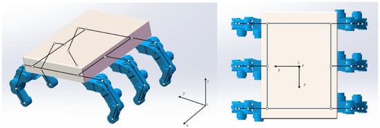
Figure 6.
The optimal pose of a hexapod robot.
The distance between the initial pose , and the target pose , of the robot refer to the sum of the squares of the distances between their respective supporting legs and feet. Assuming , , the distance between two poses can be calculated as follows:
Since the purpose of robot pose adjustment is to improve the flexibility and stability of a robot, it is therefore necessary to find the pose with the best coordination of flexibility and stability among all the poses of the hexapod robot under the current support situation. This pose is the closest to the reference pose among all robot poses and can be defined as the optimal adjustment pose.
For a given support polygon, the optimal pose of the robot refers to maintaining the support polygon unchanged: the pose with the minimum distance from the reference pose, provided that the contact point between the supporting foot and the ground does not move. Therefore, the pose adjustment of the robot is the process of adjusting the current pose to the optimal pose while keeping the supporting polygon unchanged, which can be vividly described by virtual springs, as shown in Figure 7. The red pose in the figure represents the optimal pose of the robot, while the blue pose represents the current pose of the robot. The black pose is the pose state of the robot that is closest to the optimal pose after adjusting from the current pose.
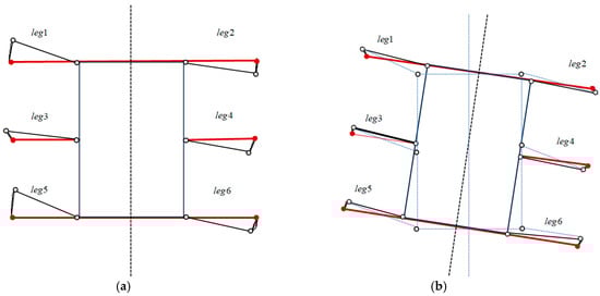
Figure 7.
Representation from the current pose to the optimal pose. (a) The current pose of the robot. (b) Target pose adjusted by the robot.
The hexapod robot in the figure has fixed footholds, with the reference pose (depicted by the thin solid line) rigidly attached to the torso. A virtual spring model is implemented between the foot endpoints of the current pose and the reference pose, where the spring tension follows Hooke’s law (linear stiffness proportional to displacement). This system inherently converges to the minimum elastic potential energy state. When the spring-driven adjustments equilibrate (the robot’s pose stabilizes), the configuration achieving minimal potential energy corresponds to the optimal pose. So, under the action of spring tension, the robot’s pose will be adjusted towards reducing the potential energy of the spring. The pose with the minimum potential energy of the spring is the optimal pose of the hexapod robot, which is the target pose that needs to be adjusted. The objective function is as follows:
where is the -th leg and is the number of robot legs. From the above three equations, it can be obtained that the various components of the gradient vector of at are as follows:
The same method can be used to obtain the various components of the gradient vector of the robot in the target pose . When the hexapod robot is in the optimal pose, takes the minimum value, and at this point the gradient components of the function will be equal to zero. The optimal pose of a hexapod robot can be solved using the gradient descent method. The gradient descent, also known as the steepest descent, has an iterative algorithm formula:
is a sequence generated according to an iterative algorithm, is the step size, and is the unit vector of the negative gradient . Select the current pose as the initial point, , and give an allowable error, . Iterate until all components of the gradient vector are close to 0. At this point, the corresponding values of each pose component are the obtained robot’s target pose, .
The position coordinates of the foot end of the current pose, P, in the geodetic coordinate system are known as , and this coordinate value remains unchanged during pose adjustment.
The current pose, P, has been adjusted to the target pose, Q. The position coordinate, , of the foot end of a hexapod robot in its torso coordinate system is fixed to the torso with reference to the pose during pose adjustment. Therefore, the reference pose foot position, , in the torso coordinate system changes with the adjustment of the pose. However, the absolute coordinate of the foot position in the geodetic coordinate system remains unchanged during the adjustment process. The pose transformation matrix of the torso coordinate system of a hexapod robot relative to the earth coordinate system can be obtained, and the following can be obtained:
where is the coordinate of the origin of the torso coordinate system in the geodetic coordinate system, represents the forward rotation angle of two coordinate systems along the coordinate axis, indicating the change in the torso pose, and is the target pose parameter of the quadruped robot.
The foot end coordinates, , in the geodetic coordinate system are known, and the foot end coordinates, , in the torso coordinate system at the optimal pose are as follows:
Using the aircraft body coordinate system as a reference coordinate system, it multiplies with the adjacent D-H transformation matrix. The transformation matrix, , from the foot coordinate system to the body coordinate system is obtained as follows:
From Equations (12) and (13), the coordinate value, , of the foot in the torso coordinate system at the optimal posture can be obtained. According to Equations (14) and (15), according to the kinematic analysis of a single leg, the relationship between the joint angle, , and the corresponding leg joint angle, , is as follows:
Thus, the rotation angles for all leg joints of the hexapod robot are computed. Leveraging these values for the angular position control of the joints enables the overall pose adjustment.
Figure 8 exemplifies adjustments from current to optimal poses. Dashed lines represent pre-adjustment poses; solid lines denote post-adjustment configurations. This pose adjustment rotates the robot’s torso to achieve coordinated motion between the torso and legs. The hexapod optimal pose method adjusts the entire robot pose—including center of gravity position and torso orientation, enhancing stability and flexibility. However, stability cannot be guaranteed with fewer supporting legs.
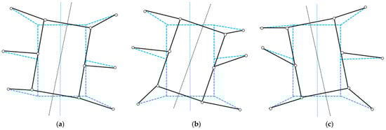
Figure 8.
Pose adjustment of hexapod robot. (a) Adjustment of quadruped front position. (b) Adjustment of tripod front position. (c) Adjustment of bipedal front position.
2. Method for Adjusting the Pose of Hexapod Robots
The pose adjustment of hexapod robots requires real-time adjustment based on complex terrain conditions, so it is necessary to discuss the pose adjustment methods of robots in different terrains. For hexapod robots walking on flat ground, high maneuverability and stability margins are required for faster speeds. On complex irregular terrain, slower walking necessitates pose adjustments primarily to enhance walking stability. The center of gravity and optimal pose adjustment methods exhibit complementary advantages and limitations. Consequently, a terrain-distinguishing pose control strategy integrating both methods is proposed.
The three adjustment methods are fused to deal with different situations during the robot walking process, as shown in Figure 9. As shown in the figure, the pose vector, , of the current position of the robot fuselage is obtained by using the pose sensor, which can be determined by the pose vector value of the current position of the robot fuselage. When is 0, the pitch angle and roll angle of the robot are zero, which means that the robot body crawls on the horizontal ground, therefore it is judged that the current ground is horizontal terrain. When is 0, it means that the body of the robot crawls on the slope. When is not 0, it means that the initial position and posture of the robot are irregular, and the robot moves in rugged terrain. The initial standard position is determined, and the initial coordinates, , of each leg can be determined according to the pose vector of the fuselage. Then, according to the active control of the robot leg crawling parameters, the coordinates of each foot end of the robot relative to the geodetic coordinate system after each crawling can be determined. According to the correlation between the known foot coordinates and the pose vector, , of the target fuselage for pose adjustment, the adjustment angle of each supporting foot joint is obtained through an inverse kinematics solution, so as to achieve the effect of driving the robot to reach the target pose, and finally realize the pose adjustment of the hexapod robot.
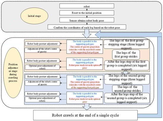
Figure 9.
Posture adjustment process of a hexapod robot.
At this time, the three-legged gait is adopted. When the robot is supported by three legs at the beginning of the robot’s step, in order to reduce the interference of the swinging leg on the pose adjustment, the posture adjustment of the fuselage and the position adjustment of the center of gravity can be implemented. To enhance robot stability, body pose adjustment and optimal pose realignment are implemented during the six-leg support phase following step completion. The method implements phased active pose optimization to adjust fuselage pose and center of gravity position during the three-leg support period (initial three-leg stance when walking commences), leveraging the brief statically stable interval for pre-adjustment. At the beginning of the swing leg movement, the interference to the adjustment is minimized. The robot will actively tilt the fuselage to make it parallel to the supporting foot polygon, which can make the robot lift the center of gravity on the convex ground to avoid scratching, and reduce the fuselage on the concave ground to increase stability. Then, the center of gravity projection of the robot is shifted in advance to the direction of the swinging leg that is about to touch the ground. After the active pre-compensation of the walking leg is completed, the leg is swung. At this time, the body and legs of the robot move forward in linkage. Compared with the traditional method, the simple swinging leg has more smooth motion and stability, and it will also reduce the jitter in the process of the robot swinging a leg. At the end of the six-legged support period, the optimal pose algorithm will recalculate the support polygon based on the actual height difference of the landing point, and then adjust the optimal pose. The robot can automatically adjust the resultant force direction from the fuselage to the end of each foot on the convex ground, avoid single-leg suspension or overload, and reduce the unreasonable jitter or mutation of the robot. This strategy significantly improves the dynamic stability of the robot in the transition phase of action switching, enhances the terrain adaptability, optimizes the overall energy efficiency, controls the active attitude of the tripod support phase, and realizes the coordination of two-stage pose optimization, making up for the limitations of the traditional single-stage adjustment method.
This method mitigates slipping and toppling risks. Fuselage pose adjustment aligns the robot parallel to the support polygon, preventing single-leg suspension or overload. During the three-leg support phase, center of gravity pre-shift maintains high stability margins throughout the leg swing, reducing rollover/slip probabilities while attenuating ground impact forces upon swing leg touchdown. Concurrently, six-leg support phase pose optimization realigns all legs toward optimal configurations, enhancing overall maneuverability and stability while minimizing sliding tendencies.
2.1. Pose Adjustment of Robots in Regular Terrain
(1) When a hexapod robot travels on horizontal terrain, the pitch angle, roll angle, and center of gravity height in the robot pose vector, , remain unchanged, so the robot’s pose adjustment only requires adjusting the horizontal position, , of the robot’s center of gravity and the yaw angle, , of the torso. So, the pose transformation matrix of the torso coordinate system relative to the geodetic coordinate system is as follows:
Firstly, adjust the hexapod robot to be parallel to the plane of the supporting foot’s foothold. At this point, the ground is horizontal, and regardless of the number of supporting feet, the supporting plane is parallel to the horizontal plane. Therefore, the value of in the body pose vector, , is 0, and the value of remains unchanged from its original value.
Secondly, during the swinging process of the robot leg, it is necessary to adjust the robot to the maximum stable margin position. Align the robot’s center of gravity with the inscribed center of its support polygon, constructed based on the current supporting legs of the hexapod system. If the support polygon at this time is a triangle, then let the coordinates of the three support legs at this time be . The three side lengths of the supporting polygon are , and the inner coordinates, , of the supporting polygon can be obtained from Equation (6) as follows:
In scenarios where the hexapod robot is supported by four or five legs, the radius of the incircle (the maximum attainable shortest distance from the centroid to all edges) within the support polygon reaches its peak value. Projection of the center of gravity onto this incircle centroid enables the robot to achieve maximum static stability. Under these specific four- or five-leg support phases, the corresponding support polygons manifest as convex quadrilaterals and pentagons, respectively. Therefore, it is necessary to convert the supporting polygons at this time into a triangle, and then calculate the inscribed circle of the converted triangle. If the converted inscribed circle is inside the corresponding supporting polygon, then the center, , of the inscribed circle is the maximum stable margin position of the corresponding supporting foot of the hexapod robot. Figure 10 shows the inscribed circles of various supporting polygons, where the center of the circle represents the maximum stability margin of the supporting polygon.
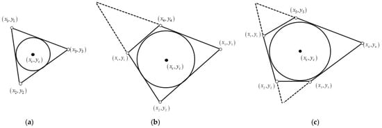
Figure 10.
Maximum stability margin of the center of the inscribed circle supporting various polygons. (a) Inscribed circle center of triangle. (b) Inscribed circle center of quadrilateral. (c) Inscribed circle center of pentagon.
Therefore, it is necessary to maintain the original values of and in the pose vector, , of the aircraft body. Thus, all values of the target pose vector, , of the aircraft relative to the geodetic coordinate system are determined, and, during the adjustment process, the position coordinate, , of the foot relative to the geodetic coordinate system remains unchanged from its original value. The relationship between the two is as follows:
According to the above formula, the coordinate value, , of the supporting end in the torso coordinate system during the swinging process can be obtained, and the corresponding leg joint angle, , can be obtained using inverse kinematics. Thus, the multi-legged robot can be adjusted to the optimal position with a large stability margin.
Additionally, during the hexapod support phase, the robot must be adjusted to its optimal pose—defined as the pose demonstrating minimal deviation from the reference pose within the set of feasible robot poses.
In addition, during the hexapod support process of the robot, it is necessary to adjust the robot to the target pose. the target pose is the pose that is closest to the reference pose among all robot poses. At this point, the expression for the target pose and the reference pose is as follows:
The necessary and sufficient condition for to obtain the minimum value in the equation is that each component of its gradient, , is zero, so the following are the case:
From the above equation and its gradient, , with zero components, the following can be solved:
Since the foot coordinates, , in the geodetic coordinate system are known, the coordinates of the foot end in the torso coordinate system at the optimal pose are . The relationship between the two is shown in Equation (19), and substituting into it is as follows:
Thus, the value in the body pose vector, , is obtained, where the value of remains unchanged and the value of is 0. Thus, all values of the target pose vector, , of the aircraft relative to the geodetic coordinate system were determined. During the adjustment process, the position coordinate, , of the foot relative to the geodetic coordinate system remains unchanged from its original value. The coordinate value, , of the supporting end in the torso coordinate system during the swinging process can be obtained, and the corresponding leg joint angle, , can be obtained using inverse kinematics. Thus, the multi-legged robot can be adjusted to the optimal pose state.
Robots typically employ a tripod gait with a duty cycle approaching 0.5 for regular terrain. However, stable walking necessitates transitional six-leg support phases during alternating leg swing sequences, increasing the duty cycle beyond 0.5. During leg swings, center of gravity shifts destabilize pose adjustment. Therefore, optimal pose adjustment should be executed exclusively during hexapod support phases. When the robot is supported on three legs, to reduce the influence of swinging legs, the center of gravity position of the robot can be adjusted to improve its stability. Furthermore, if the swinging leg for the next step is known, the center of gravity of the robot can be moved in advance to the center of the polygon formed by the supporting leg for the next step before lifting the leg. Thus, when the swinging leg is just lifted, the hexapod robot has the maximum stability margin.
The dashed line in Figure 11 represents the lifting leg of the robot. Figure 11a shows the initial pose of the robot; Figure 11b shows the robot moving its center of gravity ahead of time to the center of the polygon formed by the supporting legs before performing the next step of swinging and lifting the legs; Figure 11c shows the swinging process of the first set of legs in the quadruped gait swing of the robot, with the legs indicated by the dashed line being the swinging legs; Figure 11d shows the optimal pose adjustment of the robot after the first leg swing is completed; Figure 11e shows the robot moving its center of gravity ahead of schedule to the center of the polygon formed by the supporting legs before the second leg swing and leg lift; Figure 11f shows the swinging process of the second set of legs in the quadruped gait swing of the robot, with the legs indicated by the dashed line being the swinging legs; and Figure 11g shows the optimal pose adjustment of the robot after the second leg swing is completed, returning to the initial pose of the robot.
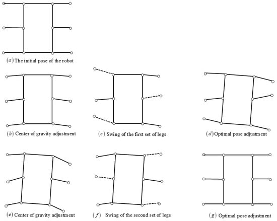
Figure 11.
Position adjustment during the three-leg gait forward process of the robot.
(2) When walking on inclined structured terrain, hexapod robots focus on their adaptability to complex terrains. Therefore, when the hexapod robot walks on an inclined road surface, the posture adjustment of the robot keeps the posture of the torso parallel to the inclined road surface, thereby improving the maneuverability of the robot, as shown in Figure 12. The angle of the slope in the figure is , the center of gravity of the robot is , and the projection of the robot’s center of gravity is .
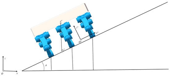
Figure 12.
The posture of the robot in the slope coordinate system.
Establish a coordinate system based on a slope, which is a coordinate system rotated by an angle, , around the Y-axis with the geodetic coordinate system. The coordinate transformation matrix from the inclined plane reference system to the geodetic coordinate system is as follows:
At this time, the hexapod robot is in the slope coordinate system, which is similar to the robot walking on a horizontal road surface in the slope coordinate system. The pitch angle, roll angle, and center of gravity height of the robot in the pose vector, , of the slope coordinate system remain unchanged, so pose adjustment only requires adjusting the horizontal position, , of the robot’s center of gravity and the yaw angle, , of the torso. So, the pose transformation matrix of the torso coordinate system relative to the slope coordinate system is as follows:
Firstly, adjust the hexapod robot to be parallel to the supporting end plane, that is, parallel to the water slope. Therefore, it is necessary to set the value of in the aircraft pose vector, , in the slope coordinate system to 0, while keeping the value of unchanged.
Secondly, based on the support legs of the multi-legged robot, the maximum stability margin position of the corresponding support legs for the inclined plane of the hexapod robot is constructed, which is the center, , position of the inscribed circle of the support polygon.
But at this point, there is an angle, , between the center of gravity of the robot and the support surface, which is equivalent to the value of in the body pose vector, , of the robot in the slope coordinate system being the calculated inner coordinate, , of the support polygon plus an offset value:
Therefore, it is necessary to adjust the pose vector, , of the robot body, . The value remains unchanged from its original value. Thus, all values of the target pose vector, , of the aircraft relative to the slope coordinate system were determined, and during the adjustment process the position coordinate, , of the foot relative to the geodetic coordinate system remained unchanged from its original value. The relationship between the two is as follows:
According to the above formula, the coordinate value, , of the supporting end in the torso coordinate system and the corresponding leg joint angle, , can be obtained during the swinging process, thereby achieving the adjustment of the multi-legged robot to the maximum stable margin position.
Furthermore, during the hexapod support phase, the robot must be realigned to its optimal pose—defined as the target pose exhibiting minimal deviation from the reference pose within the space of kinematically feasible robot poses. The mathematical expression governing this target pose relationship is as follows:
The necessary and sufficient condition for to obtain the minimum value in the equation is that each component of its gradient, , is zero:
From the above equation and the equation where the components of gradient are zero, the following can be solved:
Due to the fact that the pose adjustment of the optimal pose method is aimed at the situation of hexapod support, the reference pose during hexapod support is axisymmetric with respect to the robot. Therefore, there are and . From the relationship between the foot end and the position coordinate, , in the geodetic coordinate system, the following can be concluded:
Thus, all values in the body pose vector, , were determined. During the adjustment process, the value of the position coordinate, , of the foot relative to the geodetic coordinate system remains unchanged from its original value. The coordinate value, , of the supporting end in the torso coordinate system during the swinging process can be obtained, and the corresponding leg joint angle, , can be obtained, thus achieving the adjustment of the multi-legged robot to the optimal pose state on the inclined plane.
2.2. Pose Adjustment of Robots on Irregular Terrain
When traversing highly rugged terrain, a hexapod robot employs a dual-stage adaptive strategy: three-legged-phase pre-compensation and six-legged-phase reconstruction. This methodology converts terrain irregularities into calibrated pose adjustment parameters, demonstrating superior adaptability in uneven environments compared to flat terrain operations. During the initial three-legged support phase, the robot actively aligns its chassis with the support polygon plane through controlled body tilting. This maneuver elevates the center of gravity on convex terrain to mitigate ground interference while lowering the chassis on concave surfaces to optimize stability through increased ground contact. The center of gravity projection of the robot is shifted in advance to the direction of the swinging leg that is about to touch the ground. It is equivalent to completing the “active pre compensation” of terrain disturbance in the process of robot leg swing, so as to avoid sudden attitude change after the end of leg swing. During the six-legged support phase concluding a step cycle, the optimal pose adaptation algorithm recalibrates the support polygon using measured terrain elevation differentials. This algorithm achieves chassis alignment with the reconstructed support polygon plane prior to robot pose optimization. On convex terrain, autonomous limb loading vector redirection prevents single-leg detachment or force overloads by dynamically redistributing resultant forces across all foot end contact points. Conversely, concave terrain triggers chassis height reduction coupled with pitch angle refinement to achieve center of gravity stabilization within the support polygon’s incircle centroid region.
Through phased dynamic posture regulation, this approach surpasses traditional methods by delivering enhanced walking stability while significantly mitigating fuselage instability risks. This is achieved via the real-time compensation of swing leg disturbances through center of gravity pre-adjustment. During terminal hexapod support, landing point elevation measurements enable the instantaneous computation of optimal fuselage inclination and orientation parallel to the support surface. Consequently, joint peak torque reduction prevents single-leg suspension or overload conditions. The increased adjustment success rate in unstructured environments provides critical capabilities for search-and-rescue robots during debris navigation and military vehicles executing rollover prevention maneuvers.
As shown in Figure 13, the robot is on an irregular blue ground. In the six legs of a hexapod robot, there are three-legged support legs when walking with a three-legged gait. Therefore, the angle between the plane formed by the three-legged support feet, , and the horizontal plane, , is the normal vector which is related to the following:
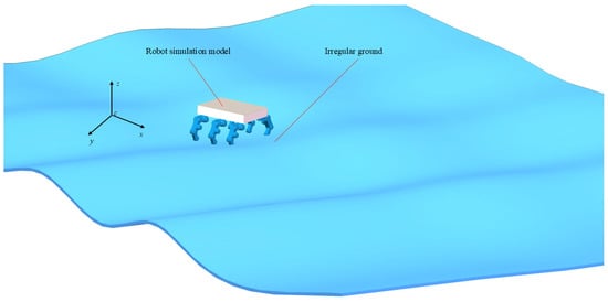
Figure 13.
Robots on irregular terrain.
In the formula, is the direction angle, which is the angle between the projection of the normal vector, , on the plane of the geodetic coordinate system and the axis.
Adjust the hexapod robot to be parallel to the supporting end plane, so the values of in the body pose vector, , in the supporting polygon coordinate system need to be and respectively. The value remains unchanged from its original value.
When walking with a bipedal gait, there are four supporting feet, and the angles between the two planes formed by the three supporting feet, , and the horizontal plane, , can be used to establish an angle of plane . By using the forward kinematics method and the angle, , between plane and contact , the pose angle of the hexapod robot’s torso relative to the earth coordinate system is solved, and the value of is obtained.
When walking with a single-foot gait, there are five supporting feet, and the angles between the three planes formed by the three supporting feet, , , , and the horizontal plane, , , , can be established as an angle, , of plane .
By using the forward kinematics method and connecting the angles and between plane , the pose angle of the hexapod robot’s torso relative to the earth coordinate system is solved, and the value of is obtained.
Secondly, based on the support legs of the multi-legged robot, the maximum stability margin of the corresponding support legs of the hexapod robot on the supporting polygon plane is constructed, which is the position of the center, , of the inscribed circle of the supporting polygon.
But at this point, there is an angle, , between the center of gravity of the robot and the support surface, which is equivalent to the value of in the body pose vector, , of the robot in the geodetic coordinate system being the calculated inner coordinate, , of the support polygon plus an offset value.
The relationship between and the invariant is maintained, thus obtaining the value of , , in :
Thus, all values of in the target pose vector, , of the aircraft relative to the geodetic coordinate system are determined. According to the same method and using inverse kinematics to obtain the corresponding leg joint angle, , the multi-legged robot can be adjusted to the maximum stable margin position.
In addition, during the hexapod support process of the robot, it is necessary to adjust the robot to the optimal pose. At this point, the target pose is the pose that is closest to the reference pose among all robot poses. At this point, the expression for the target pose and the optimal pose is as follows:
The necessary and sufficient condition for to obtain the minimum value in the equation is that each component of its gradient, , is zero, that is, there is the following:
Due to the fact that the pose adjustment based on the optimal pose strategy is aimed at the case of hexapod support, the reference pose during hexapod support is axisymmetric with respect to the robot, hence , . From the relationship between the foot end and the position coordinate, , in the geodetic coordinate system, the following can be concluded:
The pose, , of the hexapod robot under inclined structured terrain can be obtained, and the coordinate value, , of the supporting end in the torso coordinate system during the swinging process can be obtained. The corresponding leg joint angle, , can be obtained through inverse kinematics calculation, realizing the adjustment of the multi-legged robot to the optimal pose state on irregular ground.
3. Experiment and Verification of Pose Adjustment for Hexapod Robots
To validate the established posture control strategy for the hexapod robot, this approach integrates posture regulation into the robot’s gait-planning architecture. Simulation experiments were conducted to verify posture control performance during locomotion. The posture control strategy is implemented via posture adjustment methods, which operate through precise joint angle position commands. Given this joint-level actuation mechanism, direct verification in Adams is feasible. A dynamic model was built in Adams alongside a robot posture control system in Simulink, with validation achieved through Adams–Simulink co-simulation experiments.
Since XYZ displacement deviation directly indicates positioning accuracy and trajectory tracking capability, excessive deviation may cause the robot to deviate from its target path, collide with obstacles, or lose balance. Postural attitude reflects trunk balance maintenance effectiveness—abnormal attitudes induce center of gravity drift, uneven load distribution, and potential overturning. The stability margin quantifies the safety buffer against tipping, with terrain-specific margins critically determining operational safety as the fundamental reliability safeguard. The energy consumption rate evaluates locomotion efficiency, practicality, and endurance. Consequently, XYZ displacement deviation, postural attitude, stability margin, and energy consumption rate constitute the evaluation metrics, collectively assessing multi-legged robots’ core performance. These interdependent and indispensable indicators holistically validate how posture adjustment strategies cooperatively optimize accuracy, disturbance rejection, safety, and energy efficiency in complex terrains.
3.1. Simulation Results and Analysis of Pose Adjustment Under Regular Terrain
The simulation model is based on the hexapod robot model. Firstly, set the rigid body, motion pair, gravity, and ground constraints of the robot model in the Adams environment; a simulation experimental model of the hexapod robot was established, as shown in Figure 14.
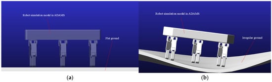
Figure 14.
Adams simulation model of a hexapod robot in different terrains. (a) Hexapod robot in regular terrain. (b) Hexapod robot in irregular terrain.
Hexapod robot locomotion is achieved by controlling individual joint motions through programmed joint angle functions. This requires the comprehensive consideration of walking stability and directional characteristics in structured terrains. During experimental verification, the hexapod robot executes linear travel using a triangular gait on a horizontal plane, maintaining a 0.7 duty cycle with fully synchronized dual-tripod motion sequences. When pose adjustment is not included in the gait of the hexapod robot, its continuous motion is shown in Figure 15. As shown in the figure, the hexapod robot without pose adjustment cannot correct the deviation in the direction of motion in a timely manner, resulting in the accumulation of directional errors and ultimately deviating from the predetermined trajectory.
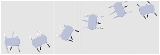
Figure 15.
Simulation walking of the triangular gait of a hexapod robot without adjustment.
The motion trajectory of the robot after adding pose adjustment is shown in Figure 16. Following each gait cycle distribution, the hexapod robot executes posture adjustment to compensate for directional deviation and correct heading. Integrating posture regulation into gait planning ensures locomotion along predefined trajectories while continuously repairing motion-induced posture errors, thereby establishing robust directionality maintenance capabilities.
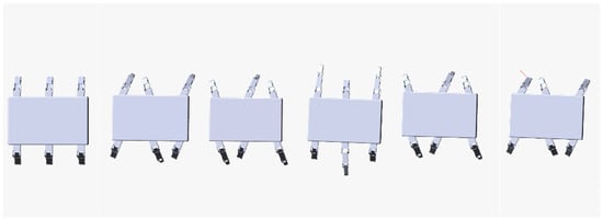
Figure 16.
Simulated walking of the adjusted hexapod robot with triangular gait.
The pose adjustment of a hexapod robot walking with a triangular gait for one cycle can be seen from Figure 17. Figure 17f shows the initial pose and final pose of the robot during the pose adjustment cycle; Figure 17a shows the robot moving its center of gravity ahead of time to the center of the polygon formed by the supporting legs before performing the next step of swinging and lifting the legs; Figure 17b shows the swinging process of the first set of legs in the quadruped gait swing of the robot, with the legs indicated by the dashed line being the swinging legs; Figure 17c shows the robot in a hexapod supported state after the first leg swing is completed. The robot is subjected to optimal pose adjustment, and the pose-adjusted robot has good directionality and an ample stability margin, with a reasonable distribution of legs and good flexibility; Figure 17d shows the robot moving its center of gravity ahead of schedule to the center of the polygon formed by the supporting legs before the second leg swing and leg lift; Figure 17e shows the swinging process of the second set of legs in the quadruped gait swing of the robot, with the legs indicated by the dashed line being the swinging legs; and Figure 17f shows the robot in a hexapod supported state after the second leg swing is completed. The robot undergoes optimal pose adjustment and returns to its initial pose. The robot after posture adjustment has good directionality and an ample stability margin, with reasonable leg distribution and good flexibility.
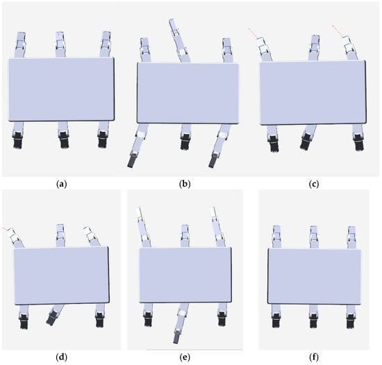
Figure 17.
Position adjustment during one gait cycle of a hexapod robot. (a) Center of gravity adjustment. (b) Swing of the first set of legs. (c) Optimal pose adjustment. (d) Center of gravity adjustment. (e) Swing of the second set of legs. (f) Optimal pose adjustment.
The curve changes during the pose adjustment process of each base joint of the hexapod robot shown in Figure 18. The 0–10 s in Figure 18 represent the process of adjusting the center of gravity, corresponding to the center of gravity adjustment of the robot before the next step of swinging and lifting the leg in Figure 17a. The 10–20 s in Figure 18 represent the process of swinging the legs, corresponding to Figure 17b, which shows the swinging process of the first set of legs in the robot’s three-legged gait swing. The 20–30 s in Figure 18 are the process of optimal pose adjustment, corresponding to Figure 17c, where the robot is in a hexapod supported state after the first leg swing is completed, and the robot undergoes optimal pose adjustment. The 30–40 s in Figure 18 correspond to Figure 17d, where the robot adjusts its center of gravity before performing the second swing leg lift. The 40–50 s in Figure 18 correspond to the swing process of the second leg of the robot’s three-legged gait swing shown in Figure 17e. The 40–50 s in Figure 18 correspond to Figure 17f, where the robot is in a hexapod supported state after the second leg swing is completed, and the optimal pose adjustment is performed on the robot.
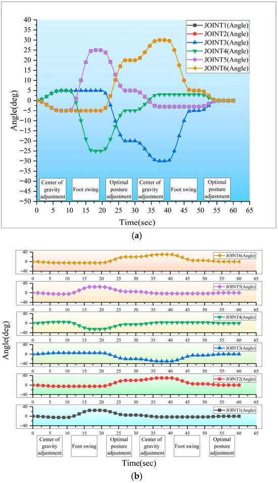
Figure 18.
Basic joint angles during the pose adjustment process of a hexapod robot. (a) Changes in the basic joint angle of the robot leg during the adjustment process. (b) The basic joint angles of the six legs of the robot.
Figure 19 and Figure 20 show the pose changes of a hexapod robot crawling on regular terrain. The red curves depict variations in postural angles and multi-directional displacements with active posture adjustment, while the blue curves represent variations without such intervention. Pose regulation in the hexapod reduces displacements along the y/z axes and confines energy consumption within a bounded range, enhancing trajectory adherence and motion stability. Within identical timeframes, the regulated system achieves greater locomotion distance. Critical attitude angles (pitch/yaw/roll) are actively constrained, enforcing straight-line locomotion. Unregulated systems exhibit progressively accumulated lateral displacement and yaw angle errors, culminating in significant orbital deviation.
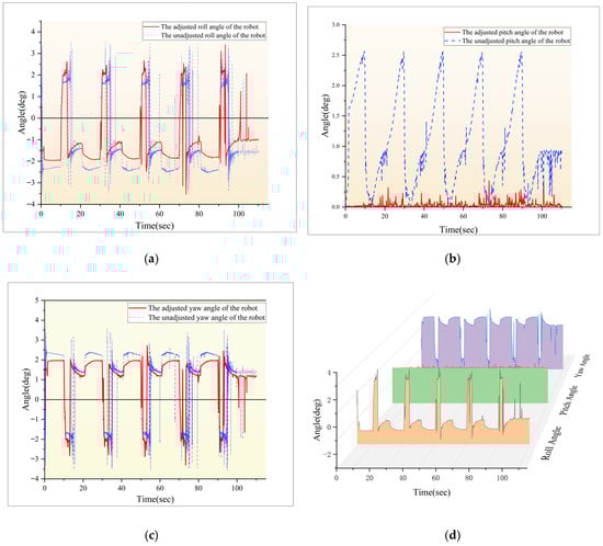
Figure 19.
Comparison of Euler angles before and after pose adjustment of a hexapod robot. (a) Roll angle curves before and after robot pose adjustment. (b) Pitch angle curves before and after robot pose adjustment. (c) Yaw angle curves before and after robot pose adjustment. (d) All angle curves before and after robot pose adjustment.
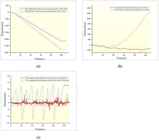
Figure 20.
Comparison of X–Y–Z-direction offset values before and after pose adjustment of a hexapod robot. (a) Displacement in the X-direction before and after robot pose adjustment. (b) Offset distance in the Y-direction before and after robot pose adjustment. (c) Offset distance in the Z-direction before and after robot pose adjustment.
The changes in the stability margin curve of the hexapod robot before and after pose adjustment can be obtained from Figure 21. The red line segment in the figure represents the change curve of the stability margin of the adjusted robot during movement, which is also the distance of the robot’s center of gravity projected onto the supporting polygon. The blue line segment represents the stable margin variation curve of the robot after adjustment. During the movement of the robot, the supporting polygon and center of gravity of the robot will change with the movement and have a certain correlation with the gait. By adding pose adjustment to the robot during its movement, it can be seen from the figure that when the stability margin of the robot is too small, the pose adjustment of the robot can maintain the stability margin at a relatively high value, thereby ensuring the stability of the robot during its movement.
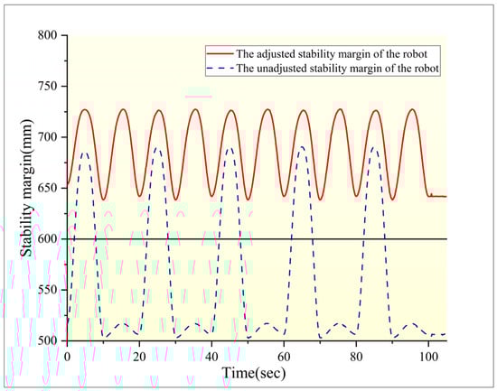
Figure 21.
Stability margin curve of a hexapod robot before and after pose adjustment.
Figure 22 shows the joint energy dissipation curves before and after pose adjustment of a hexapod robot. Figure 22a shows the three types of joints without posture adjustment and the total energy consumption during the robot’s motion process; Figure 22b shows the three types of joints without posture adjustment and the total energy consumption during the robot’s motion process; and Figure 22c–f show the comparison of the energy effects of the base joint, knee joint, ankle joint, and total sum of robot motion with and without attitude adjustment, respectively. The upper part of the graph represents the curve without posture adjustment, while the lower part represents the curve with posture adjustment added. Due to the attitude adjustment added during the robot’s motion, the offset values in the X–Y–Z-directions and the additional offsets in the pitch, yaw, and roll angles can be reduced, thereby reducing unnecessary motion and improving the robot’s operational efficiency. From the figure, it can be concluded that the energy consumption of the robot’s base joints, knee joints, and ankle joints is lower compared to the energy consumption without posture adjustment.
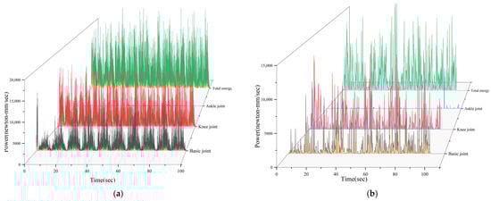
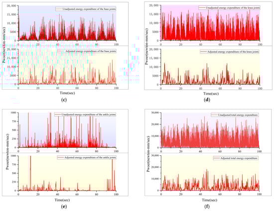
Figure 22.
Joint energy consumption curve of a hexapod robot before and after pose adjustment. (a) Unadjusted energy expenditure of the joints. (b) Adjusted energy expenditure of the joints. (c) Energy expenditure of the basic joints. (d) Energy expenditure of the knee joints. (e) Energy expenditure of the ankle joints. (f) Energy expenditure of all the joints.
3.2. Simulation Results and Analysis of Pose Adjustment in Irregular Terrain
During hexapod robot locomotion on irregular terrain, terrain specificity necessitates prioritized gait selection criteria: walking stability supersedes forward characteristics as the primary consideration. When traversing horizontally irregular terrain, pose adjustment first horizontally reorients the torso before optimizing residual pose parameters via a combination of a pose optimization strategy and center-of-gravity adjustment. The center of gravity of the hexapod robot is adjusted to be parallel to the supporting polygon, and the rotation angles of each joint can be directly solved through inverse kinematics. Then, by controlling the position of the joints, the torso of the hexapod robot can be adjusted to stability.
Figure 23 shows the comparison of the corresponding torso pose parameters before and after adjustment. As shown in the figure, when a hexapod robot without attitude control moves forward in irregular terrain, the Y-direction offset changes significantly, which can easily cause the robot to move off course. In addition, the pitch angle, yaw angle, and roll angle of the robot will change with its movement on the ground in irregular terrain. From the enlarged views in Figure 23d–f, it can be seen that the alternating legs during the robot’s movement cause peak fluctuations in the pitch angle, yaw angle, and roll angle of the robot. After adding pose adjustment, the peak fluctuation deviation of the torso can be repaired in a shorter time, while also avoiding the impact of pose deviation on the robot’s next movement. The instantaneous fluctuation of the robot’s pose at the thin solid line display is more obvious, mainly due to the adverse consequences caused by the uncorrected peak fluctuation deviation. By comparison, it can be found that pose adjustment can correct the peak deviation of pose fluctuations in a timely manner, enabling the robot’s pose to fluctuate within a smaller range while avoiding other negative effects caused by pose deviations, ensuring the robot’s efficiency and stability.
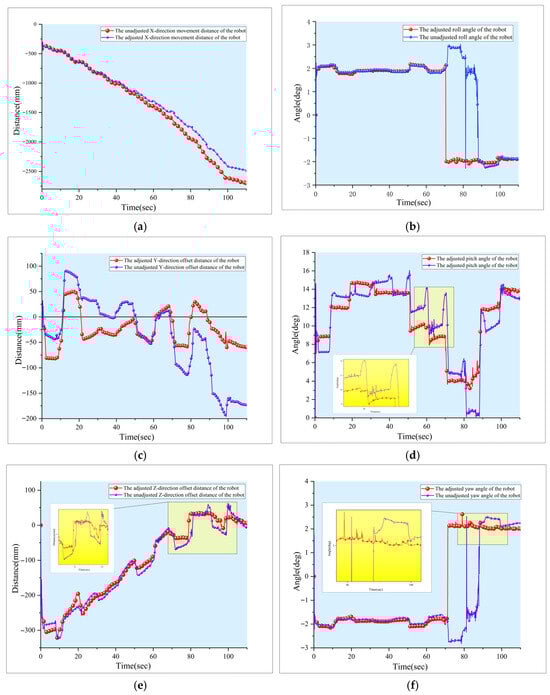
Figure 23.
Curve comparison of pose parameters before and after adjustment of a hexapod robot. (a) Displacement in the X-direction before and after robot pose adjustment. (b) Roll angle curves before and after robot pose adjustment. (c) Offset distance in the Y-direction before and after robot pose adjustment. (d) Pitch angle curves before and after robot pose adjustment. (e) Offset distance in the Z-direction before and after robot pose adjustment. (f) Yaw angle curves before and after robot pose adjustment.
The stability margin and energy consumption of robots during their movement in irregular terrain can be obtained from Figure 24. The robot is in the process of moving. Adding pose adjustment to the robot during its motion, the pose adjustment is performed when the stability margin of the robot is too small, to maintain the stability margin of the robot at a relatively high value, thereby ensuring the stability of the robot during motion. In addition, it can be seen from Figure 24b that, after attitude adjustment, the robot reduced unnecessary movement such as robot offset, and the energy consumption of the robot was lower compared to the energy consumption without attitude adjustment, which improved the operating efficiency of the robot.
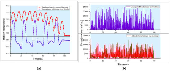
Figure 24.
Stability margin and energy consumption of robots. (a) Stability margin curve of a hexapod robot before and after pose adjustment. (b) Energy expenditure of all the joints before and after robot pose adjustment.
3.3. Physical Prototype Verification
A physical prototype is built to verify the simulation effect. The prototype is placed in irregular terrain to keep walking for 25 moving cycles. The data of the prototype is obtained and compared to verify the effect of the robot pose adjustment method.
The attitude adjustment process of the hexapod robot prototype during a complete cycle of executing a triangular gait can be obtained from Figure 25. Figure 25f shows the initial posture of the robot, which is also the posture at the end of the cycle; Figure 25a shows the process of transferring the center of gravity to the center of the polygon formed by the next supporting leg before the robot prepares to lift the next leg; Figure 25b shows the swinging motion of the first set of legs in the quadruped gait of the robot; and Figure 25c shows that after the first set of leg swings is completed, the robot is in a hexapod support state and has undergone optimal posture adjustment, resulting in the better directionality and stability of the robot. The leg layout is reasonable and the flexibility is enhanced; Figure 25d shows the process of transferring the center of gravity to the center of the polygon formed by the next supporting leg before the robot prepares to lift the second leg; Figure 25e shows the swinging motion of the second set of legs during the quadruped gait of the robot; and Figure 25f once again shows that after the second set of leg swings is completed, the robot is in a hexapod support state and has undergone optimal posture adjustment, returning to its initial posture At this point, the robot has better directionality and stability, reasonable leg layout, and enhanced flexibility.
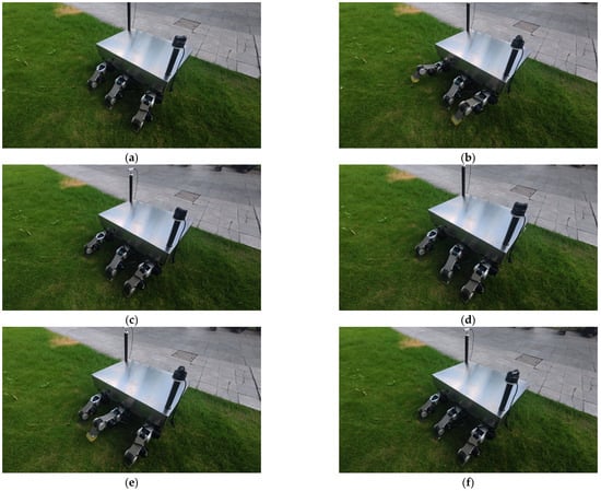
Figure 25.
Position adjustment of a hexapod robot prototype in one gait cycle. (a) Center of gravity adjustment. (b) Swing of the first set of legs. (c) Optimal pose adjustment. (d) Center of gravity adjustment. (e) Swing of the second set of legs. (f) Optimal pose adjustment.
Figure 26 shows the motion process of the hexapod robot prototype with pose adjustment added. Figure 26c,h,k, and n show the robot keeping the body parallel to the supporting polygon formed by the landing point of the supporting foot. Figure 26e and m show the process of the robot adjusting its center of gravity before swinging its legs, transferring the center of gravity to the center of the polygon formed by the next set of supporting feet. Figure 26g,i,l, and o represent the optimal pose adjustment of the robot after swinging its legs.
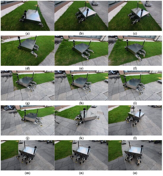
Figure 26.
Motion process of introducing pose adjustment into a hexapod robot prototype. (a) Robot motion process 1. (b) Robot motion process 2. (c) Robot motion process 3. (d) Robot motion process 4. (e) Robot motion process 5. (f) Robot motion process 6. (g) Robot motion process 7. (h) Robot motion process 8. (i) Robot motion process 9. (j) Robot motion process 10. (k) Robot motion process 11. (l) Robot motion process 12. (m) Robot motion process 13. (n) Robot motion process 14. (o) Robot motion process 15.
Figure 27 shows the comparison of the torso pose parameters of the robot prototype before and after adjustment. From Figure 27a–c, it can be seen that leg movements produce significant instantaneous peak fluctuations in the pitch angle, yaw angle, and roll angle during the gait alternation of the robot. After introducing posture adjustment, the peak deviation of these torso parameters can be quickly corrected in a short period of time, effectively preventing the accumulation of deviation from affecting subsequent gait movements. The blue line marked in the figure shows obvious instantaneous fluctuations in posture, which is a direct consequence of the failure to correct peak deviation in a timely manner. Comparative experiments have shown that attitude adjustment can efficiently suppress the amplitude of attitude transients and constrain robot attitude changes within a smaller range. This not only eliminates the adverse effects of peak fluctuations themselves, but also ensures the overall smoothness and efficiency of robot motion.
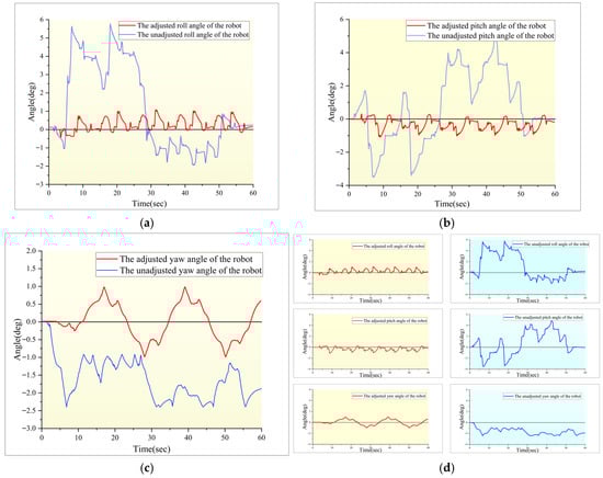
Figure 27.
Comparison of Euler angles before and after adjustment of a robot prototype. (a) Roll angle curves before and after robot pose adjustment. (b) Pitch angle curves before and after robot pose adjustment. (c) Yaw angle curves before and after robot pose adjustment. (d) All angle curves before and after robot pose adjustment.
The hexapod robot attitude control framework, developed through Adams–Simulink co-simulation and prototype experimental validation, integrates joint angle/position control with triangular gait planning to enable real-time attitude correction and optimization during locomotion. This strategy executes optimal pose adjustments during the support phase of each gait cycle, incorporating the preemptive projection of the center of gravity toward the subsequent support polygon prior to swing leg actuation. During the tripod support phase initiating each step, the robot actively tilts the torso to align with the support foot polygon—elevating the center of gravity on convex terrain to prevent ground contact interference, while lowering the torso on concave terrain to enhance stability. Subsequent preemptive center of gravity shifting toward the swing leg touchdown direction, coupled with active leg pre-compensation, enables linked torso–leg kinematics during swing leg execution. Compared to traditional isolated leg swing approaches, this coordinated mechanism achieves enhanced motion smoothness and stability while minimizing swing-phase oscillations. At the termination of the hexapod support cycle, the optimal pose algorithm dynamically recalculates the support polygon based on landing point elevation discrepancies, enabling real-time attitude recalibration. This allows the automatic adjustment of foot end resultant force vectors on convex terrain to prevent single-leg detachment or overload, while mitigating abrupt torso jerking. Foot contact point positional variance induces support polygon calculation errors, which may propagate heading deviations under extreme terrain irregularity. Center of gravity estimation latency may further induce torso pitch overshoot, critically reducing stability margins and incurring rollover risks during dynamic load transients. Corrective center of gravity redistribution and pose optimization during incipient slip/rollover phases can restore stability margins to operational thresholds, arresting instability progression. Failure to implement timely corrections during acute rollover scenarios precipitates system failure. Experimental validation confirms that this methodology enhances directional fidelity and trajectory precision by eliminating cumulative heading deviations, ensuring linear path adherence. Stability augmentation is achieved through optimized center of gravity positioning and load distribution, sustaining high stability margins. Additional benefits include improved energy efficiency via reduced joint/whole-body power consumption and superior terrain adaptability, particularly in compensating pitch/yaw/roll transients and suppressing Y/Z-axis positional drift. The closed-loop attitude control architecture provides an effective solution for stable hexapod navigation in complex environments.
4. Conclusions
This study develops a hierarchical pose control framework for hexapod heavy-duty robots, integrating real-time center of gravity optimization, virtual spring-based attitude synchronization, and multi-modal terrain adaptation to ensure stable locomotion in complex environments. By dynamically aligning the zero moment point with the support polygon’s maximal stability region, the system achieves continuous center of gravity repositioning while a gradient descent-driven virtual spring mechanism synchronizes torso–foot coordination during hexapod support phases. Finally, the effectiveness of the entire strategy was verified on horizontal, sloping, and irregular terrain through Adams–Simulink joint simulation and physical prototype experiments. Through the phased position and attitude collaborative optimization technology, the pre-compensation and optimal attitude adjustment during the three-legged support period can reduce the vibration energy of the fuselage, reduce unreasonable jitter or mutation, and reduce the risk of secondary collapse in ruin environments in search-and-rescue missions. In a military transportation scenario, the trafficability of extreme terrain is significantly improved. The balanced optimization of contact force in the six-legged stage will improve the passing rate of muddy swamps, and reduce the probability of rollover and slip under load with the dynamic center of gravity control.
This study proposes a center of gravity attitude co-optimization strategy addressing critical limitations in conventional hexapod heavy-duty robot control, specifically stability flexibility tradeoffs and error-induced energy inefficiencies. The methodology elevates three core competencies: Stability enhancement through maximum stability margin center of gravity presetting and virtual spring pose optimization maintains operational safety thresholds, drastically reducing full-system tipover risks. Trajectory precision improvement via five-cycle continuous locomotion trials on planar/inclined surfaces demonstrates consistent lateral error suppression and linear path adherence. Energy efficiency optimization achieved by minimizing redundant leg oscillations and corrective maneuvers reduces aggregate joint power expenditure while sustaining gait cycle temporal efficiency across operational modes. Prototype validation through 25 uninterrupted gait cycles in heterogeneous terrains confirms algorithmic robustness against real-world complexities, with demonstrable capabilities in pose deviation compensation and disturbance rejection. The synergistic center of gravity posture adjustment mechanism concurrently achieves trajectory fidelity maintenance, energy consumption reduction, and anti-interference performance enhancement, proving particularly effective in maintaining operational reliability in search/rescue operations and military-grade terrain negotiation scenarios.
The proposed pose adjustment methodology has demonstrated experimental efficacy while exhibiting limitations regarding complex environmental uncertainties and practical implementation constraints. Current assumptions include predefined terrain stiffness, measurable foot–terrain contact, and exclusive reliance on offline planning for static gait cycles, omitting dynamic impact coupling, soft soil subsidence effects, and high-mobility gait integration. Algorithmic real-time performance on embedded systems remains suboptimal. Future work will integrate online terrain estimation with adaptive model predictive control, incorporate vision–force fusion feedback, extend applicability to dynamic gaits (running, obstacle negotiation), and advance multi-objective optimization, balancing energy efficiency with safety constraints. These enhancements aim to bolster system stability and task adaptability in mission-critical scenarios, including disaster response and military logistics. Building upon gait-phase-dependent control architecture, this work will design a hierarchical dual-model predictive control (dual-MPC) framework. During tripod support phases, the dual-MPC embeds active exploration objectives to achieve real-time fuselage attitude and center of gravity adjustments while learning terrain mechanical parameters to minimize swing leg disturbances [36]. In hexapod support phases, adaptive MPC executes global optimal pose optimization while prospectively planning subsequent gait strategies using historically learned data [37]. This unified framework integrates dynamic parameter-learning weight adaptation with stochastic MPC robust constraint handling, validating stability enhancement effects and online learning efficiency across slope and soft soil unstructured terrains.
Author Contributions
Conceptualization, C.Y. and D.F.; methodology, C.Y.; software, C.Y.; validation, X.L., D.F. and C.Y.; formal analysis, C.Y.; investigation, D.F.; resources, D.F.; data curation, X.L.; writing—original draft preparation, C.Y.; writing—review and editing, X.L.; visualization, C.Y.; supervision, D.F.; project administration, D.F.; funding acquisition, X.L. All authors have read and agreed to the published version of the manuscript.
Funding
This research received no external funding.
Data Availability Statement
The original contributions presented in the study are included in the article, further inquiries can be directed to the corresponding author.
Conflicts of Interest
The authors declare no conflict of interest.
References
- Li, Y.; Guo, Y.; An, T.; Zhu, M.; Ma, B. Gait coordination control of bipedal modular reconfigurable robot based on adaptive neural network. Trans. Inst. Meas. Control 2025, 47, 2063–2075. [Google Scholar] [CrossRef]
- Namura, N.; Nakao, H. A central pattern generator network for simple control of gait transitions in hexapod robots based on phase reduction. Nonlinear Dyn. 2025, 113, 10105–10125. [Google Scholar] [CrossRef]
- Zhao, D.; Liu, J.; Yang, P.; Cui, T.; Wu, D.; Zhang, L. Modeling and stability control of steering and reconfiguration motion for wheel-legged metamorphic robot. Proc. Inst. Mech. Eng. Part C J. Mech. Eng. Sci. 2025, 239, 4256–4272. [Google Scholar] [CrossRef]
- El Nagar, A.M.; Abdrabou, A.; El Bardini, M.; Elsheikh, E.A. A class of embedded fuzzy PD controller for robot manipulator: Analytical structures and stability analysis. Soft Comput. 2025, 29, 4423–4428. [Google Scholar] [CrossRef]
- Korayem, M.H.; Namdarpour, F.; Lademakhi, N.Y. Hybrid Stable Adaptive Control Approach for Navigation of Nonholonomic Wheeled Mobile Robots on Slippery Surfaces with Obstacles. Int. J. Control Autom. Syst. 2025, 23, 1542–1550. [Google Scholar] [CrossRef]
- Sha, H.; Guo, R.W.; Zhu, X.; Miao, Z. Cooperative Adaptive Consensus Tracking Control for Multiple Wheeled Mobile Robot Systems with Model Uncertainties and External Disturbances. Int. J. Robust Nonlinear Control 2025, 35, 3533–3544. [Google Scholar] [CrossRef]
- Xu, K.; Wang, S.; Shi, L.; Li, J.; Yue, B. Horizon-stability control for wheel-legged robot driving over unknow, rough terrain. Mech. Mach. Theory 2025, 205, 105887. [Google Scholar] [CrossRef]
- Noce, A.L.; Patanè, L.; Arena, P. A stable and safe method for two-leg balancing of a quadruped robot using a neural-network-based controller. Robot. Auton. Syst. 2025, 186, 104901. [Google Scholar] [CrossRef]
- Yamasaki, J.; Lyu, S.; Morishita, K.; Saito, K. Gait and cost of transport analysis for quadruped robot with neuromorphic integrated circuit. Artif. Life Robot. 2024, 30, 227–235. [Google Scholar] [CrossRef]
- Li, S.; Wang, H.; Li, D.; An, J.; Zhang, X.; Tian, J.; Niu, J. Research on gait generation and gait conversion of (2UPS-U) +R series-parallel hybrid wheel-legged quadruped robot. Proc. Inst. Mech. Eng. Part C J. Mech. Eng. Sci. 2024, 238, 5833–5850. [Google Scholar] [CrossRef]
- Pan, Y.; Zhang, L.; Mei, D.; Tang, G.; Ji, Y.; Tan, K.; Wang, Y. Gait and simulation analysis of quadruped crawling robot based on metamorphic structure. Ind. Robot Int. J. Robot. Res. Appl. 2024, 51, 91–104. [Google Scholar] [CrossRef]
- Jiang, Z.; Wang, Y.; Wang, S.; Bi, S.; Chen, J. Motion Planning and Control with Environmental Uncertainties for Humanoid Robot. Sensors 2024, 24, 7652. [Google Scholar] [CrossRef]
- Khan, M.S.; Mandava, R.K.; Panchore, V. Optimizing PID control for enhanced stability of a 16-DOF biped robot during ditch crossing. J. Field Robot. 2024, 42, 559–583. [Google Scholar] [CrossRef]
- Guo, T.; Zhang, X.; Li, J.; Song, D.; Liu, X. Innovative active disturbance motion control for an underwater adsorption wall-climbing robot with uncertainties and compensations. Ocean Eng. 2024, 311, 118916. [Google Scholar] [CrossRef]
- Yu, L.; Xiong, J.; Xie, M. Iterative-learning-based tracking control of a two-wheeled mobile robot with model uncertainties and unknown periodic disturbances. J. Frankl. Inst. 2024, 361, 106962. [Google Scholar] [CrossRef]
- Cheng, H.; Wang, X. Research on stability control strategy of adjustable pressure wall-climbing robot based on adsorption identification. Proc. Inst. Mech. Eng. Part C J. Mech. Eng. Sci. 2024, 238, 1590–1602. [Google Scholar] [CrossRef]
- Han, M.; Xiong, B.; Liu, J.; Yang, D.; Li, T. Research on time-energy optimal trajectory planning of articulated heavy-duty robot. Proc. Inst. Mech. Eng. 2024, 238, 9630–9643. [Google Scholar] [CrossRef]
- Zhu, H.; Xing, H.; Zhu, J.; Zhang, P. Design of Fuzzy Gait Control Algorithm for Multi-legged Hydraulic Robot. IAENG Int. J. Comput. Sci. 2023, 50, 1042. [Google Scholar]
- Song, D.; Ji, H.; Yin, G. Attitude stability control system of mobile robot mechanism based on nanosensor. J. Control Decis. 2023, 10, 13–18. [Google Scholar] [CrossRef]
- Xu, K.; Lu, Y.; Shi, L.; Li, J.; Wang, S.; Lei, T. Whole-body stability control with high contact redundancy for wheel-legged hexapod robot driving over rough terrain. Mech. Mach. Theory 2023, 181, 105199. [Google Scholar] [CrossRef]
- Sun, Y.; Chen, X.; Wang, Z.; Qin, H.; Jing, R. Adaptive interval type-2 fuzzy control for multi-legged underwater robot with input saturation and full-state constraints. Int. J. Syst. Sci. 2023, 54, 2859–2874. [Google Scholar] [CrossRef]
- Fang, L.; Wang, T.; Zheng, W.; Liu, Z.; Ming, L.; Zheng, X.; Wu, M. Consistency optimal coordination control of underground heavy-load robot in nonstructural environment. Robot. Auton. Syst. 2023, 159, 104281. [Google Scholar] [CrossRef]
- Yang, Y.; Wang, J.; Shi, L.; Li, J. Gait Simulation Research of 2-DOF Lower Limb Rehabilitation Robot Based on ADAMS and MATLAB. J. Phys. Conf. Ser. 2022, 2414, 012020. [Google Scholar] [CrossRef]
- Wei, S.; Wu, H.; Liu, L.; Zhang, Y.; Chen, J.; Li, Q. A CPG-based gait planning and motion performance analysis for quadruped robot. Ind. Robot 2022, 49, 779–797. [Google Scholar] [CrossRef]
- Liao, F.; Zhou, Y.; Zhang, Q. Gait transition and orbital stability analysis for a biped robot based on the V-DSLIP model with torso and swing leg dynamics. Nonlinear Dyn. 2022, 108, 3053–3075. [Google Scholar] [CrossRef]
- Ito, K.; Yoshizawa, K. URARAKA VI: Multi-legged robot with suckers to climb walls and pipes. Artif. Life Robot. 2022, 27, 834–841. [Google Scholar] [CrossRef]
- Sun, Y.; Dou, G.; Duan, W.; Chen, X.; Zheng, J.; Xin, L.; Bai, L. Involute-arc-leg for Multi-legged Robot: High Stability and Low Energy Consumption. Mech. Mach. Theory 2022, 170, 104701. [Google Scholar] [CrossRef]
- Nima, M.; Onur, Ö. Gait and locomotion analysis of a soft-hybrid multi-legged modular miniature robot. Bioinspir. Biomim. 2021, 16, 066009. [Google Scholar]
- Ozkan-Aydin, Y.; Goldman, D.I. Self-reconfigurable multilegged robot swarms collectively accomplish challenging terradynamic tasks. Sci. Robot. 2021, 6, eabf1628. [Google Scholar] [CrossRef]
- Muñoz, F.; Cervantes-Rojas, J.S.; Valdovinos, J.M.; Sandre-Hernández, O.; Salazar, S.; Romero, H. Dynamic Neural Network-Based Adaptive Tracking Control for an Autonomous Underwater Vehicle Subject to Modeling and Parametric Uncertainties. Appl. Sci. 2021, 11, 2797. [Google Scholar] [CrossRef]
- Soltanpour, M.R.; Zaare, S.; Haghgoo, M.; Moattari, M. Free-Chattering Fuzzy Sliding Mode Control of Robot Manipulators with Joints Flexibility in Presence of Matched and Mismatched Uncertainties in Model Dynamic and Actuators. J. Intell. Robot. Syst. 2020, 100, 47–69. [Google Scholar] [CrossRef]
- Wang, Y.; Chen, Z.; Zu, H.; Zhang, X.; Mao, C.; Wang, Z. Improvement of Heavy Load Robot Positioning Accuracy by Combining a Model-Based Identification for Geometric Parameters and an Optimized Neural Network for the Compensation of Nongeometric Errors. Complexity 2020, 2020, 5896813. [Google Scholar] [CrossRef]
- Yu, H.; Sun, Q.; Wang, C.; Zhao, Y. Frequency response analysis of heavy-load palletizing robot considering elastic deformation. Sci. Prog. 2020, 103, 36850419893856. [Google Scholar] [CrossRef]
- Long, Z.; Zhang, B.; Guo, S. Control Strategy for Hydraulic Hybrid Servo Drive System of Heavy Load Robot. Mater. Sci. Forum 2014, 3256, 521–525. [Google Scholar] [CrossRef]
- You, B.; Qiao, M.; Xu, J.; Liu, D. Low-Speed Control of Heavy-Load Transfer Robot with Long Telescopic Boom Based on Stribeck Friction Model. Math. Probl. Eng. 2012, 2012, 432129.1–432129.12. [Google Scholar] [CrossRef]
- Hu, J.; Yan, P.; Tan, G. A two-layer optimal scheduling method for microgrids based on adaptive stochastic model predictive control. Meas. Sci. Technol. 2025, 36, 026208. [Google Scholar] [CrossRef]
- Tan, G.; Hua, W.; Yang, C.; Tran, X.T.; Li, Z. Dual control for autonomous airborne source search with Nesterov accelerated gradient descent: Algorithm and performance analysis. Neurocomputing 2025, 630, 129729. [Google Scholar] [CrossRef]


Disclaimer/Publisher’s Note: The statements, opinions and data contained in all publications are solely those of the individual author(s) and contributor(s) and not of MDPI and/or the editor(s). MDPI and/or the editor(s) disclaim responsibility for any injury to people or property resulting from any ideas, methods, instructions or products referred to in the content. |
© 2025 by the authors. Licensee MDPI, Basel, Switzerland. This article is an open access article distributed under the terms and conditions of the Creative Commons Attribution (CC BY) license (https://creativecommons.org/licenses/by/4.0/).