Residual Attention-Driven Dual-Domain Vision Transformer for Mechanical Fault Diagnosis

Abstract

Traditional fault diagnosis methods, which rely on single-vibration signals, are insufficient for capturing the complexity of mechanical systems. As neural networks evolve, attention mechanisms often fail to preserve local features, which can reduce diagnostic accuracy. Additionally, transfer learning using single-domain metrics struggles under fluctuating conditions. To address these challenges, this paper proposes an innovative adversarial training approach based on the Time–Frequency Fused Vision Transformer Network (TFFViTN). This method processes signals in both the time and frequency domains and incorporates a robust attention mechanism, along with a novel metric that combines Wasserstein distance and maximum mean discrepancy (MMD) to precisely align feature distributions. Adversarial training further strengthens domain-invariant feature extraction. Experiments on bearing and gear datasets demonstrate that our model significantly improves diagnostic performance, stability, and generalization.

1. Introduction

Bearings and gears serve as key components in rotating machinery and are widely used in aerospace, transportation, wind energy, and industrial manufacturing [1,2,3]. Continuous operation and surface degradation may cause faults [4], leading to downtime or severe failures [5]. Accurate identification plays a vital role in ensuring operational reliability and reducing maintenance cost [6]. Vibration signal-based approaches have become an important means for evaluating the health state of machinery [7], supporting predictive maintenance and improving operational efficiency [8].

Recent advances in deep learning have strongly promoted progress in intelligent fault diagnosis [9]. Studies focusing on feature extraction have made notable contributions [10]. Huang et al. [11] combined convolutional neural networks (CNNs) and long short-term memory (LSTM) to alleviate time-related delays and improve diagnostic performance. Jiang et al. [12] introduced a multi-sensor fusion-driven semi-supervised prototypical contrastive learning (PCL) framework for changing conditions with limited labels. Chen et al. [13] integrated wavelet transform, CNNs, and extreme learning machine (ELM) to enhance classification accuracy. Hu et al. [14] designed a multi-scale autoencoder with a generative adversarial network (GAN) to obtain depth-sensitive features. Li et al. [15] proposed an attention-improved CNN (AT-ICNN) for strengthened feature representation. Cross-domain adaptation has also attracted attention. Wu et al. [16] constructed a knowledge dynamic matching unit-guided multi-source domain adaptation network with an attention mechanism (KDMUMDAN) for multi-source adaptation. Qian et al. [17] improved feature alignment through improved joint distribution adaptation (IJDA). Zhao et al. [18] introduced the subdomain adaptation capsule network (SACNet) to reduce subdomain confusion. Noise suppression research has further improved diagnosis under challenging environments. Li et al. [19] enhanced stochastic resonance for low-SNR scenarios. Xu et al. [20] proposed the global contextual feature aggregation network (GCFAN) to extract robust features under fluctuating conditions. Collectively, these studies contribute to progress in feature extraction, domain adaptation, and robust modeling.

Despite these advances, several challenges remain. First, relying on only time-domain or frequency-domain signals restricts the diversity of extracted features, and the representations lose essential complementary information. Second, deeper attention-based networks tend to emphasize global patterns, reducing sensitivity to localized fault cues and weakening feature diversity. Third, single-domain distance metrics struggle to capture complex domain variations, making it difficult to obtain domain-agnostic representations under unseen conditions. To address these limitations, this study designs a cross-domain fault diagnosis framework that integrates time–frequency fusion, residual attention, and a hybrid domain distance metric. The contributions are summarized as follows:

(1)

A unified input scheme combines time-domain and frequency-domain signals to enhance complementary feature acquisition and improve reliability under varying and fluctuating conditions.

(2)

A residual attention module transmits shallow attention responses to deeper layers, improving local feature perception and maintaining stable feature diversity.

(3)

A dual-metric alignment strategy integrates Wasserstein distance and MMD, capturing domain variations from complementary viewpoints and enhancing the extraction of domain-agnostic representations.

The remainder of this paper is arranged as follows: Section 2 presents the theoretical foundation, Section 3 describes the proposed framework, Section 4 reports the experimental evaluation, and Section 5 summarizes the conclusions.

2. Theoretical Background

2.1. Multiple Self-Attention Mechanism

Self-attention allows a network to model internal feature relationships that traditional feed-forward layers cannot capture. For fault diagnosis, this mechanism highlights correlations among signal features, enabling the model to assign greater weight to more informative elements, as illustrated in Figure 1a.

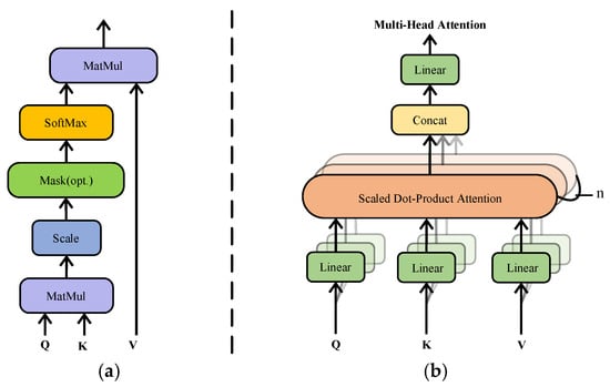
Figure 1. Comparative illustration of conventional versus multi-head self-attention frameworks. (a) Classic self-attention architecture. (b) Multi-head self-attention architecture.

Given an input feature matrix $X=\{x_1,x_2,\dots ,x_n\}$, three linear projections generate query (Q), key (K), and value (V) matrices through learnable parameters:

$$Q=X·W^q, K=X·W^k, V=X·W^v$$

(1)

where $W_Q,W_K,W_V\in {\mathbb{R}}^{N\times D_k}$ are learnable projection matrices and $d_k$ is the subspace dimension for each head.

The attention relevance is determined using a scaled dot product, normalized by the feature dimension $d$ and then processed through a Softmax function to generate weight coefficients:

$$S_l={\displaystyle \frac{Q·K^T}{\sqrt{d_k}}}$$

(2)

$$A_l=Softmax\left(S_l\right)$$

(3)

where $S_l\in {\mathbb{R}}^{N\times \mathrm{N}}$ is the pairwise score matrix and $\sqrt{d_k}$ provides scale normalization.

The aggregated output is obtained as:

$$\widetilde{X_l}=A_l·V_l$$

(4)

where $\widetilde{X_l}\in {\mathbb{R}}^{N\times d_k}$ represents the attended values for each token.

To capture richer dependencies, multiple attention heads are employed, as shown in Figure 1b. This approach enhances the ability of the model to focus on different aspects of the data simultaneously, improving its fault diagnosis capabilities.

$${head}_i=\mathrm{S}\mathrm{o}\mathrm{f}\mathrm{t}\mathrm{m}\mathrm{a}\mathrm{x}\left({\displaystyle \frac{Q_i·{K_i}^T}{\sqrt{d_k}}}\right)V_i, i=1,\dots ,H$$

(5)

$$\mathrm{M}\mathrm{u}\mathrm{l}\mathrm{t}\mathrm{i}\mathrm{H}\mathrm{e}\mathrm{a}\mathrm{d}\left(Q,K,V\right)=\mathrm{C}\mathrm{o}\mathrm{n}\mathrm{c}\mathrm{a}\mathrm{t}\left({head}_1,{head}_2,\cdots ,{head}_n\right)W^O$$

(6)

where $H$ is head count, $Q_i,K_i, V_i\in {\mathbb{R}}^{N\times d_k}$ are the projections for head $i$, and $W^O$ is the output projection matrix that maps concatenated heads back to dimension $D$.

This parallel multi-head design enables the model to process features across various subspaces, strengthening its ability to extract discriminative information and improving robustness under complex mechanical conditions.

2.2. Residual Connection

Residual connections, first introduced by He et al. [21], are utilized to address training degradation problems in deep neural networks. They introduce shortcut pathways that directly link earlier layers to later ones, ensuring smooth gradient propagation and maintaining stable information flow. This mechanism is depicted in Figure 2.

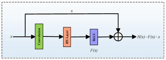
Figure 2. Residual connection process diagram.

Given an input $x$, the residual output is formulated as follows:

$$H\left(x\right)=F\left(x\right)+x$$

(7)

where $x$ is input to a block, $F\left(x\right)$ denotes the nonlinear transformation of the block, and $H\left(x\right)$ denotes the residual output that preserves original information and eases gradient flow.

This addition enables the model to learn residual mappings rather than complete transformations, simplifying optimization and improving convergence. By merging original and transformed features, residual connections preserve shallow-level information while enabling deeper layers to focus on abstract representations.

In fault diagnosis, this design enhances feature continuity across network layers and reduces the risk of gradient vanishing, allowing deeper networks to be effectively trained. Consequently, the diagnostic model achieves higher precision, stability, and efficiency in identifying mechanical faults.

2.3. Domain Distance

Domain distance describes the degree of divergence between the source and target domains in transfer learning. It reflects the extent to which feature representations differ when operating conditions, sensor configurations, or surrounding environments change. A smaller domain distance indicates stronger cross-domain correlation, allowing more reliable knowledge transfer. A larger distance suggests substantial domain shift, which can lead to reduced diagnostic accuracy or even negative transfer.

In mechanical fault diagnosis, domain distance corresponds to variations in vibration signal patterns induced by changes in speed, load, or noise. These variations alter the underlying data characteristics and hinder generalization across domains. Accurately assessing and reducing domain distance is therefore essential for forming domain-invariant representations and improving diagnostic adaptability. Streamlining domain disparity harmonizes feature attributes extracted from multiple domains and supports a more stable diagnostic outcome under diverse operational conditions.

3. Time–Frequency Fused Vision Transformer Network (TFFViTN)

3.1. System Overview

To overcome the limitations of single-signal analysis, which often fails to fully capture the operational state of equipment, along with issues like feature globalization in deep networks and the inadequate robustness of single-domain distance metrics, this research introduces an improved Vision Transformer framework for intelligent fault identification. The method employs a hybrid time–frequency signal representation, allowing the model to extract richer and more discriminative information about the operational behavior of the machine. Additionally, to bolster feature alignment across disparate domains, a dual-domain approach merges the Wasserstein and MMD metrics. This clever integration boosts the responsiveness and dependability of the model across various cross-domain diagnostic contexts. The structure itself is a cohesive assembly of four critical parts, signal preprocessing, feature distillation, domain disparity analysis, and fault identification, as shown in Figure 3.

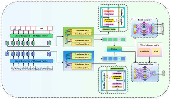
Figure 3. The framework of TFFViTN.

3.2. Concurrent Signal Processing in Time–Frequency Domain

To address limitations of using a single domain, we adopt a parallel multi-scale segmentation and energy-guided fusion strategy that integrates time-domain and frequency-domain signals while preserving multi-resolution characteristics.

(1)

Two types of signals, $X_t$ and $X_f,$ are partitioned into equal-length segments at multiple scales $P^{\left(s\right)}$($s=1,\dots ,S$), resulting in $Z_t^{\left(s\right)}$ and $Z_f^{\left(s\right)}$ subsequences, respectively. Each segment is mapped into a latent space by linear projection:

$$Z_t^{\left(s\right)}=\left\{{W_t}^{\left(s\right)}·x_i^{t,\left(s\right)}+b_t^{\left(s\right)}\right\}, Z_f^{\left(s\right)}=\left\{{W_f}^{\left(s\right)}·x_i^{f,\left(s\right)}+b_f^{\left(s\right)}\right\}$$

(8)

where $Z_t^{\left(s\right)},$ $Z_f^{\left(s\right)}\in {\mathbb{R}}^D$ are D-dimensional tokens; $x_i^{t,\left(s\right)}$ and $x_i^{f,\left(s\right)}$ denote the $i$-th segment at scale $s$; and $W$ and $b$ are learnable parameters.

(2)

To retain temporal order within each segmented sequence, sinusoidal positional encodings are applied as follows:

$$PE\left(pos,2i\right)=\mathit{sin}\left({\displaystyle \frac{pos}{{\mathrm{10,000}}^{2i/D}}}\right), PE\left(pos,2i+1\right)=\cos \left({\displaystyle \frac{pos}{{\mathrm{10,000}}^{2i/D}}}\right)$$

(9)

where $pos$ is the segment index, $i$ indexes dimension pairs, and PE has dimension $D$.

Position encodings are added to the projected features:

$${\widehat{Z}}_t^{\left(s\right)}=Z_t^{\left(s\right)}+P_t^{\left(s\right)}, {\widehat{Z}}_f^{\left(s\right)}=Z_f^{\left(s\right)}+P_f^{\left(s\right)}$$

(10)

where $P_t^{\left(s\right)},P_f^{\left(s\right)}\in {\mathbb{R}}^D$ are positional vectors for scale $s$.

(3)

For each scale $s$, local segment energies are computed as $E_t^{\left(s\right)}=\mid \mid Z_t^{\prime \left(s\right)}\mid {\mid }_2^2$ and $E_f^{\left(s\right)}=\mid \mid Z_f^{\prime \left(s\right)}\mid {\mid }_2^2$, and normalized fusion weights are derived as follows:

$${\beta }_t^{\left(s\right)}={\displaystyle \frac{E_t^{\left(s\right)}}{E_t^{\left(s\right)}+E_f^{\left(s\right)}}}, { \beta }_f^{\left(s\right)}={\displaystyle \frac{E_f^{\left(s\right)}}{E_t^{\left(s\right)}+E_f^{\left(s\right)}}}$$

(11)

where ${‖ · ‖}_{2 }$ denotes Euclidean norm over token channels, ${\beta }_t^{\left(s\right)},{ \beta }_f^{\left(s\right)}\in \left(\mathrm{0,1}\right)$ and ${\beta }_t^{\left(s\right)}+{ \beta }_f^{\left(s\right)}=1$.

The fused representation at scale $s$ is

$$Z_{fusion}^{\left(s\right)}={\beta }_t^{\left(s\right)}·{\widehat{Z}}_t^{\left(s\right)}+{\beta }_f^{\left(s\right)}·{\widehat{Z}}_f^{\left(s\right)}$$

(12)

where ${ Z}_{fusion}^{\left(s\right)}\in {\mathbb{R}}^D$ represent the fused features.

(4)

Fused features from all scales are concatenated to form the multi-scale fused feature:

$$Z_{msf}=Concat\left(Z_{fusion}^{\left(1\right)}, Z_{fusion}^{\left(2\right)},\cdots ,Z_{fusion}^{\left(s\right)}\right)$$

(13)

where $Z_{msf}\in {\mathbb{R}}^{S · D}$ is the concatenated multi-scale feature.

This strategy preserves multi-resolution characteristics and uses physically interpretable energy cues to adaptively balance the two domains, which differs from simple concatenation by introducing scale-wise adaptive weighting that enhances feature relevance under fluctuating operating conditions.

3.3. Improved Feature Extraction via Residual Attention

Under fluctuating operating conditions, rapid variations in amplitude and frequency make it difficult to preserve fault-related local fluctuations throughout the network. Although the standard Vision Transformer (ViT) captures long-range dependencies through global self-attention, deep layers often suppress fine-grained patterns and move the attention focus toward globally dominant structures. This shift can homogenize feature representations and cause feature collapse, reducing diagnostic reliability for non-stationary vibration signals where local variations usually contain the key fault cues.

To address these limitations, an enhanced residual attention mechanism is incorporated to strengthen the preservation and propagation of shallow-layer information. Figure 4a,b illustrate the contrast between the original and modified structures. Residual pathways are injected directly into each attention layer, allowing distinct local details detected in early stages to be retained and integrated into deeper semantic representations. This design enriches feature diversity and mitigates the dominance of overly globalized responses.

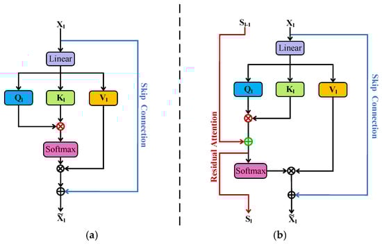
Figure 4. Diagram illustrating standard versus residual self-attention architectures. (a) Standard self-attention mechanism. (b) Residual attention mechanism.

A permutation-invariant aggregation function $\gamma$ is introduced to further improve stability. Since canonical ViT lacks translational invariance, the patch sequence may influence the attention update, especially when vibration signals are collected under fluctuating or imperfect sampling conditions. The aggregation function keeps the update consistent across rearranged or shifted patches, resulting in more stable representations. The attention score is defined as follows:

$$S_l=\left\{\begin{array}{c}{\displaystyle \frac{Q_0{K}_0^T}{\sqrt{d_0}}}, if l=0\\ \gamma \left({\displaystyle \frac{Q_l{K}_l^T}{\sqrt{d_l}}},S_{l-1}\right), otherwise\end{array}\right.$$

(14)

where $Q_0, K_0\in {\mathbb{R}}^{N\times d_k}$ are the query and key at layer 0, $\gamma (. , .)$ denotes the aggregation operator that is invariant to token permutation, and $S_{l-1}$ is the previous-layer score.

To prevent excessive shallow features from overwhelming high-level semantics, a weighting factor α is applied to regulate inter-layer information flow:

$$S_l=\left\{\begin{array}{c}{\displaystyle \frac{Q_l{K}_l^T}{\sqrt{d_l}}}, if l=0\\ \alpha \left({\displaystyle \frac{Q_l{K}_l^T}{\sqrt{d_l}}}\right)+\left(1-\alpha \right)\left(S_{l-1}\right), otherwise\end{array}\right.$$

(15)

where $\alpha$ controls the flow of information from lower layers to higher ones.

This formulation adjusts the strength of inter-layer information fusion, preventing shallow features from overwhelming higher-level representations while still preserving essential localized variations. As a result, the network achieves a more effective equilibrium between local detail retention and global context modeling.

The result of the MHSA layer is defined as follows:

$$X^{\left(l\right)}=A_l{V}_l=softmax\left(S_l\right)V_l$$

(16)

where $X^{\left(l\right)}$ is the output of the attention mechanism of the $l$-th layer and $V_l\in {\mathbb{R}}^{N\times d_k}$ are layer-$l$ values.

The feature extraction architecture incorporates several Transformer units. Within each unit, layer normalization is applied to stabilize training, while skip connections facilitate smoother information flow between layers. The mathematical representation of this transformation is as follows:

$${X^{\prime }}^{\left(l\right)}=X^{\left(l\right)}+MultiHead\left(LayerNorm\left(X^{\left(l\right)}\right)\right)$$

(17)

$$X^{\left(l+1\right)}={X^{\prime }}^{\left(l\right)}+MLP\left(LayerNorm\left({X^{\prime }}^{\left(l\right)}\right)\right)$$

(18)

where LayerNorm denotes layer normalization, MultiHead is from (6) and (7), MLP is a two-layer feed-forward block expanding the dimension by ratio $r,\mathrm{a}\mathrm{n}\mathrm{d} X^{(l+1)}$ denotes the outcome of the $l$-th block.

To prevent feature redundancy, a diversity regularizer is applied to channel activations of each block:

$$L_{div}=\sum _l\sum _{i\ne j}(Cov(H_l^{\left(i\right)},H_l^{\left(j\right)}){)}^2$$

(19)

where $H_l^{\left(i\right)}$ denotes channel $i$ activation at layer $l$, Cov denotes covariance across tokens, and the sum penalizes redundant channel correlations.

After $L$ residual-regulated blocks, the refined representation is obtained by average pooling of the final block:

$$Z_{refined}=AvgPool\left(H_L\right)$$

(20)

where $H_{L }$ is the last-layer activation tensor and AvgPool denotes global average pooling over the token dimension.

The integration of residual connections, self-attention, order-invariant aggregation, and controllable multi-layer information flow differentiates the proposed mechanism from conventional ViT variants. The design simultaneously preserves rapidly changing local patterns under fluctuating conditions, maintains global contextual cues, enhances translational invariance, and limits interference across layers. By balancing the renewal and preservation of information, the mechanism increases feature diversity, reduces redundancy, and forms a stable representation space for vibration signals, ultimately improving diagnostic accuracy and robustness in dynamic and non-stationary environments.

3.4. Dual-Domain Distance Metric

In transfer learning fault diagnosis, domain discrepancy metrics are employed to evaluate the difference between source and target feature distributions and enhance domain alignment. The Wasserstein distance effectively captures global distribution shifts but fails to describe fine-grained local variations, while MMD is sensitive to nonlinear local structures but limited in global representation. Using either metric alone leads to incomplete feature adaptation.

(1)

To achieve more balanced alignment, an adaptive hybrid domain distance is introduced, combining the strengths of both metrics. The loss functions for Wasserstein distance and MMD are defined as follows:

$$L_{WAR}={\mathbb{E}}_{x~P_s}\left[f\left(x\right)\right]-{\mathbb{E}}_{x~P_t}\left[f\left(y\right)\right]$$

(21)

$$L_{MMD}={\displaystyle \frac{1}{n^2}}\sum _{i=1}^n\sum _{j=1}^{n}k\left(x_i,x_j\right)-{\displaystyle \frac{2}{nm}}\sum _{i=1}^n\sum _{j=1}^{m}k\left(x_i,y_j\right)+{\displaystyle \frac{1}{m^2}}\sum _{i=1}^m\sum _{j=1}^{m}k\left(y_i,y_j\right)$$

(22)

where $f\left(·\right)$ is the critic function approximating Wasserstein divergence, $P_s \mathrm{a}\mathrm{n}\mathrm{d} P_t$ denote source and target feature distributions, $x_i$ represents the source samples, $y_j$ represents the target samples, $n \mathrm{a}\mathrm{n}\mathrm{d} m$ are their counts, and $k\left(\cdot ,\cdot \right)$ is a positive-definite kernel.

The hybrid loss is defined as follows:

$$L_{hd}={\mu }_W·L_{WAR}+{\mu }_M·L_{MMD}$$

(23)

where ${\mu }_{W }$ and ${\mu }_M$ control the contributions of each term. These coefficients are dynamically adjusted using gradient descent.

(2)

Instead of fixing ${\mu }_W$ and ${\mu }_M$, the model introduces a self-adjusting factor $\delta$ that dynamically reflects the dominant type of domain difference at each iteration. The weights are computed as follows:

$${\mu }_W={\displaystyle \frac{e^{-\delta }}{e^{-\delta }+e^{\delta }}}, { \mu }_W={\displaystyle \frac{e^{\delta }}{e^{-\delta }+e^{\delta }}}$$

(24)

where scalar $\delta \in \mathbb{R}$ indicates dominance between global and local discrepancy.

When global distribution shifts dominate ($\delta <0$), the Wasserstein term gains higher importance, whereas when local discrepancies are more significant ($\delta >0$), the MMD term becomes dominant.

(3)

The self-adaptive factor $\delta$ is updated through gradient descent according to the overall alignment loss:

$$\delta =\delta -\eta {\displaystyle \frac{\partial L_{hd}}{\partial \delta }}$$

(25)

where $\eta$ is the learning rate for $\mathsf{\delta }$ and gradients are computed by backpropagation.

This adaptive mechanism enables the model to automatically balance global and local domain alignment in real time, ensuring that each metric contributes appropriately during training.

(4)

By progressively minimizing the adaptive hybrid loss, the model achieves consistent domain alignment across different layers, effectively reducing distribution gaps and enhancing diagnostic robustness under fluctuating operating conditions.

Unlike approaches that directly sum multiple metrics with fixed coefficients, the adaptive weighting controlled by δ serves as a structural innovation enabling real-time balancing of global and local discrepancies.

3.5. Integrated Mechanism and Workflow Overview

The principal components operate in a coordinated manner to form a unified mechanism for feature extraction and adaptation. The time–frequency fusion produces a heterogeneous representation that retains transient variations and spectral structures, creating a comprehensive basis for subsequent processing. The residual attention module refines this representation by allocating adaptive attention weights to fault-related regions while preserving continuity through residual pathways. This design enhances sensitivity to localized variations and maintains the diversity of extracted features. The resulting representation is then evaluated by the dual-domain distance metric. The Wasserstein distance reflects geometric deviations between domains, and MMD regulates domain disparity from a complementary perspective. Their combined effect stabilizes domain alignment and retains the discriminative structures derived from the fused signals. Through this integrative process, the framework forms a feature space with improved separability, stronger robustness under fluctuating operating conditions, and more stable cross-domain diagnostic performance.

3.6. TFFViTN Algorithmic Workflow and Architectural Details

To improve reproducibility and clarify the operational flow, the core steps of the TFFViTN framework are summarized in Algorithm 1. The algorithm highlights time–frequency feature fusion, residual attention, and hybrid dual-domain distance metric modules, showing how data flows through the model for feature extraction, classification, and domain alignment.

Algorithm 1. Training procedure of TFFViTN

Input: Source-domain signals: $X_s^f$, $X_s^t$ and labels $Y_s;$    Target-domain signals: $X_t^f$, $X_t^t$;    Maximum epoch $E_{max}$;    Accuracy threshold τ;    Learning rate η

Output: Optimized feature extractor F and classifier C.

for epoch = 1 to $E_{max}$ do

1:  Sample mini-batches from source ($X_s^f$, $X_s^t$,$Y_s$) and target domains ($X_t^f$, $X_t^t$);

2:   Pass time-domain and frequency-domain signals separately through corresponding residual attention branches and extract embeddings $\left(Z_s^f,Z_{s }^t,Z_t^f,Z_{t }^t\right)$;

3:   Compute multi-scale fused representations:$f_s=Fuse\left( Z_s^f ,{ Z}_{s }^t\right),$    $f_t=Fuse\left(Z_t^f,Z_{t }^t\right)$;   4:   Predict source and target outputs: ${\displaystyle \widehat{Y_s}}=C\left(f_s\right), \widehat{Y_t}=C\left(f_t\right)$, Compute classification loss $L_{\mathrm{c}}$;   5:   Compute hybrid dual-domain alignment loss $L_d$ between $f_s$ and $f_t$ using adaptive Wasserstein + MMD;   6:   Aggregate the total loss: L = $\beta \ast L_d+\lambda$ + $L_c$   7:   Backpropagation and parameter update: Update parameters of F and C with learning rate $\eta$;   8:   Evaluate target accuracy ${Acc}_t$;   9:   If ${ Acc}_t\ge \tau$ then save model checkpoint and embedding visualization; break;  end for return: optimized parameters F, C.

The detailed architectural and hyperparameter settings for the TFFViTN framework are summarized in Table 1. These specifications ensure full reproducibility and provide clear guidance for verifying the claimed diagnostic performance.

Table 1. TFFViTN architectural and training configuration.

Item	Setting/Description
Transformer Encoder Layers	6
Attention Heads per Layer	4
Input Feature Dimension	D = 1024 (concatenated time–frequency representation)
Multi-scale Segmentation	Scales: $S=3$, segment lengths $P^{\left(1\right)},P^{\left(2\right)},P^{\left(3\right)}$
Fusion Weighting	Energy-based normalization across time and frequency domains
Residual Attention	Layer normalization + residual connections + permutation-invariant aggregation
Hybrid Domain Distance	Wasserstein + MMD with self-adaptive weighting factor $\delta$
Optimizer	Adam
Learning rate	0.001 (cosine decay schedule)
Batch size	64
Weight decay	5 × 10−4
Source/Target sampling ratio	1:1
Number of epochs	1000
Early stopping	Validation loss not improving for 10 consecutive epochs
Hardware	NVIDIA RTX 4060 GPU, Pycharm 1.6

The TFFViTN framework has been deliberately designed with computational efficiency in mind. By limiting the architecture to six Transformer layers and four attention heads per layer, the number of learnable parameters and floating-point operations is substantially reduced relative to standard ViT configurations (commonly 12–24 layers with 8–16 heads), while still maintaining sufficient capacity to capture both local and global dependencies in vibration signals. Memory usage and inference time are significantly lowered, making the model feasible for real-time deployment on industrial monitoring systems. Multi-scale segmentation and energy-guided fusion introduce only linear overhead relative to the sequence length, and the residual attention mechanism reuses intermediate representations without additional heavy computation. Overall, TFFViTN achieves a balance between diagnostic accuracy, robustness, and computational efficiency, confirming its suitability for industrial fault diagnosis under variable operating conditions.

4. Experimental Verification

4.1. Data Description of Experiment A

This study investigates the application of transfer learning for intelligent fault detection under continuously varying and unstable operating conditions. These conditions introduce significant uncertainty into vibration responses and reduce the generalization capability of diagnostic frameworks. An extensive experimental platform is constructed to assess performance in diverse mechanical scenarios. The setup simulates practical operating environments and includes a motor, coupling, rotor, bearing pedestal, gearbox, and a braking unit [22]. Vibration acceleration sensors are arranged on the bearing pedestal and the machine base to capture structural responses. Data acquisition is completed through an LMS testing system to ensure accurate and synchronized measurements, as illustrated in Figure 5.

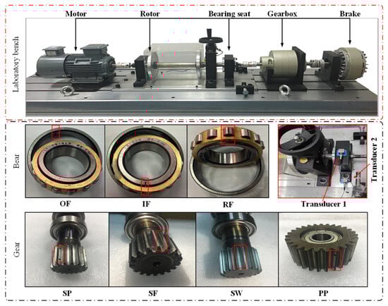
Figure 5. Experiment rig and malfunctioning components.

Two mechanical datasets are adopted to evaluate diagnostic robustness across different fault categories, one for bearings and one for gears. The bearing dataset is generated from a cylindrical roller bearing (NU205EM) under four health conditions—normal, outer race defect, inner race defect, and rolling element defect—with the rolling element defect including two severity levels to broaden the fault range. The gear dataset contains five conditions, covering normal operation as well as multiple degraded states such as pitting and cracking in the sun gear, and wear or pitting in the planetary gear. The sampling rate is set to 25.6 kHz. Each bearing dataset includes 1000 samples across the time and frequency domains. The data is divided evenly into training and testing subsets to provide a balanced and objective evaluation of diagnostic performance.

4.2. Experiment A: Fault Diagnosis Under Bearing Data

4.2.1. Data Description of Experiment A

This experiment gathers vibration measurements from a cylindrical roller bearing (NU205EM) operating under multiple dynamic conditions. The tests are carried out at three variable rotational speeds, and based on these configurations, six distinct transfer scenarios (A1–A6) are designed. Each scenario corresponds to a specific combination of speed and load variation, as outlined in Table 2, which summarizes the detailed settings for Experiment A.

Table 2. Operating condition specifications for Experiment A.

Transfer Task	Source Domain	Target Domain
	Fluctuation Speed (rpm)	Fluctuation Speed (rpm)
A1	1000~1500	1500~1800
A2	1000~1500	1800~2000
A3	1500~1800	1000~1500
A4	1500~1800	1800~2000
A5	1800~2000	1000~1500
A6	1800~2000	1500~1800

4.2.2. Comparative Evaluation of Experiment A

To evaluate the effectiveness of the proposed method (PM), researchers utilized four models for comparative analysis:

CM1: A baseline model using only time-domain input, intended to highlight the advantages of joint time–frequency feature utilization in fault diagnosis.

CM2: A baseline deep network constructed on the standard ViT framework, employing a dual-domain distance function [23]. This setup is used to examine how the enhanced model improves stability and generalization across different working conditions.

CM3: A fault diagnosis network based on the Swin Transformer, which employs window-based attention and incorporates a single-domain distance metric to quantify domain differences [24].

CM4: A fault diagnosis network based on FasterNet, which leverages streamlined convolutional operations and feature reuse techniques to improve computational efficiency and accelerate training without sacrificing accuracy [25].

CM5: A new unsupervised transfer learning framework that combines joint distribution alignment and adversarial networks [26].

CM6: A new unsupervised transfer learning method that combines structure-optimized convolutional neural networks and fast batch nuclear-norm maximization [27].

Six comparison models are used to benchmark the PM, covering single-domain baselines, Transformer-based architectures, and recent unsupervised domain adaptation techniques. This configuration ensures that both feature extraction effectiveness and domain-alignment capability can be systematically assessed. Statistical reliability is ensured by repeating each experiment ten times. The standard deviations in Table 2 confirm that PM exhibits markedly lower variance than other approaches, indicating more stable behavior under source–target domain transfer learning. To further assess the significance of improvements, paired t-tests are conducted between PM and each comparison model. The proposed method demonstrates statistically significant performance benefits (p < 0.01) over all comparison methods. In addition, one-way ANOVA performed across all seven models shows that the performance differences are highly significant (p < 0.001), further verifying that the superiority of PM is not due to random fluctuations.

4.2.3. Parameter Sensitivity Analysis

Ablation experiments are conducted to examine the influence of the parameter α on model performance. As illustrated in Figure 6, setting α to zero causes the network to depend excessively on representations from the previous layer and prevents the introduction of new information, resulting in an accuracy of 91%. When α reaches one, the network relies entirely on the attention mechanism of the current layer, and the accuracy increases to 91.9%. The best result appears at α = 0.6, where the accuracy reaches 99%. Adjacent values also maintain results above 98%, indicating stable sensitivity across a broad range.

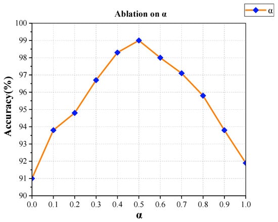
Figure 6. Influence analysis of weight factors on residual attention mechanisms.

During model training, the balance between domain discrepancy loss and classifier loss plays a key role in overall optimization. To explore their combined effect, ablation studies are performed using ten configurations of the coefficients β for domain discrepancy and λ for classification. As shown in Figure 7, the lowest accuracy of 93.8% occurs when both coefficients take small values. Accuracy rises progressively as the weights increase and reaches 99.31% at the most balanced configuration. This setting produces an effective compromise between domain alignment and classification reliability. All experiments are repeated multiple times to reduce random fluctuations and ensure consistent results.

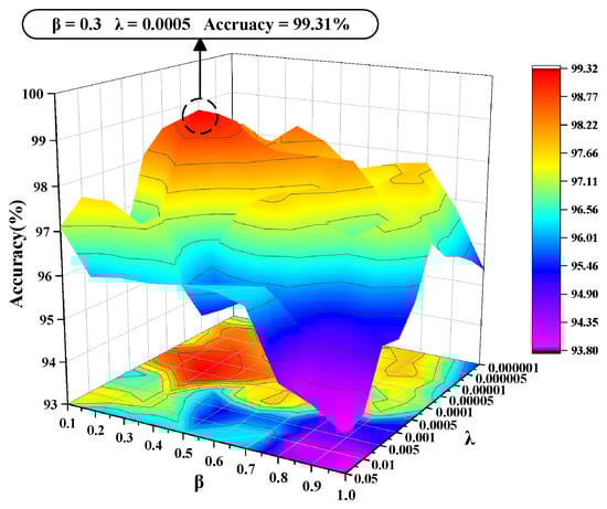
Figure 7. Analysis of the weight coefficient impact on domain discrepancy loss.

Balancing the contributions of current-layer and past-layer characteristics enhances the integration of hierarchical representations. This balance reduces redundancy in lower-level features and improves abstraction in higher-level layers, resulting in more reliable diagnostic outcomes under fluctuating operating conditions.

4.2.4. Experimental Results of Experiment A

Table 3 and Figure 8 summarize the diagnostic results of the six models. The performance improves progressively as model complexity and domain adaptation strategies advance. CM1 adopts only time-domain inputs and attains 87.5% accuracy. Its limitation stems from insufficient information because it relies on a single source rather than a combined time–frequency representation. Based on a traditional ViT, CM2 achieves 92.5% accuracy; however, its limited feature extraction capability prevents it from fully capturing complex fault patterns across different operating conditions, thereby constraining its overall performance. CM3 replaces the feature extractor with a Swin Transformer and retains a single-domain metric, reaching 94.6%. This result indicates that a single-domain metric cannot fully characterize the diversity of fault-related information. CM4 adopts FasterNet and achieves 96.1%. Although FasterNet improves efficiency and accelerates training, its performance remains constrained under unstable conditions when compared with the more adaptable strategy in the PM. CM5 and CM6 represent recent unsupervised transfer learning approaches and yield 97.1% and 97.5%. These approaches still show sensitivity to domain imbalance, reducing overall diagnostic consistency. In contrast, the PM reaches 99.08%. This improvement results from the integration of time–frequency fusion, residual attention, and adaptive domain-loss weighting, enabling stable performance under varying operating conditions.

Table 3. Diagnostic results of Experiment A.

Accuracy	CM1	CM2	CM3	CM4	CM5	CM6	PM
A1	86.72 ± 4.18	90.92 ± 3.06	93.82 ± 2.86	94.72 ± 1.81	96.20 ± 1.97	97.05 ± 1.65	98.80 ± 0.86
A2	87.17 ± 3.86	91.34 ± 2.80	95.30 ± 3.04	95.93 ± 2.36	97.11 ± 1.86	97.48 ± 1.41	99.21 ± 0.61
A3	89.41 ± 3.29	93.15 ± 2.78	94.38 ± 2.69	96.80 ± 1.63	97.34 ± 2.04	97.22 ± 1.27	99.07 ± 0.53
A4	88.94 ± 3.12	94.38 ± 2.39	94.80 ± 2.02	97.16 ± 1.87	97.85 ± 1.95	97.16 ± 1.94	99.28 ± 0.58
A5	86.45 ± 3.83	93.26 ± 3.64	93.89 ± 3.11	95.42 ± 2.57	96.95 ± 1.76	98.21 ± 1.22	99.34 ± 0.73
A6	87.36 ± 4.06	92.16 ± 3.49	95.64 ± 2.38	96.51 ± 1.85	97.25 ± 1.53	98.35 ± 1.36	98.75 ± 0.47

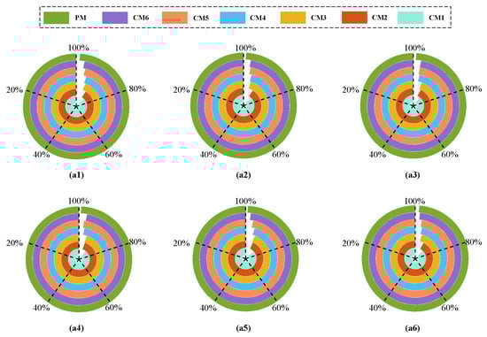
Figure 8. Performance comparison of accuracy across six transfer tasks. (a1) Accuracy for task A1. (a2) Accuracy for task A2. (a3) Accuracy for task A3. (a4) Accuracy for task A4. (a5) Accuracy for task A5. (a6) Accuracy for task A6.

Figure 9 presents a radar chart that displays the stability of the six methods. The PM forms a compact distribution with a smaller standard deviation, reflecting stable behavior across different fault categories. The even spread of accuracy values demonstrates strong resilience to variations in signal patterns and confirms consistent performance in complex environments.

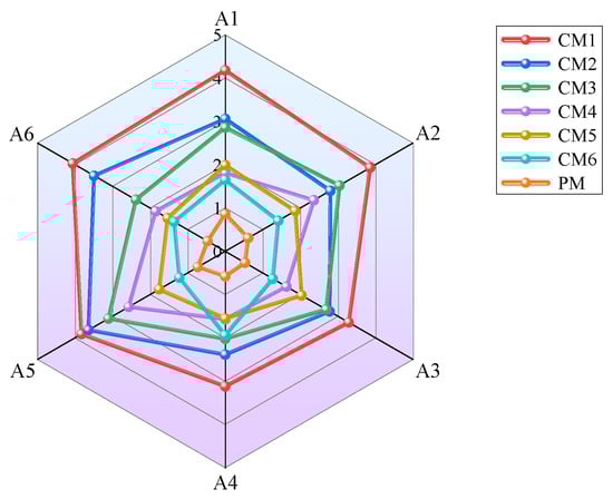
Figure 9. Standard deviation radar chart of accuracy.

Figure 10 illustrates the transfer task results of A1 using t-SNE visualization [28]. Figure 10a shows that CM1 forms only partial clusters, and the overlap between fault types such as OF0.2 and RF0.2 reveals limited separability under single-domain information. Figure 10b demonstrates that CM2 presents weak aggregation, implying incomplete feature transfer and the need for enhanced attention mechanisms and dual-domain metrics. Figure 10c indicates that the standard ViT produces insufficient feature representation, leading to misclassification in several regions. Figure 10d shows that CM4 improves fault distinction through residual attention, while the remaining single-domain metric restricts cluster quality. In contrast, Figure 10g demonstrates that the PM bridges domain gaps through the integration of multiple distance metrics and achieves strong classification robustness across all categories.

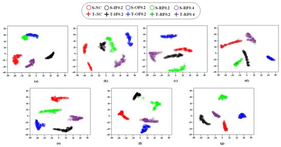
Figure 10. t-SNE feature visualization for transfer task A1. (a) Dimensionality reduction result for CM1. (b) Dimensionality reduction result for CM2. (c) Dimensionality reduction result for CM3. (d) Dimensionality reduction result for CM4. (e) Dimensionality reduction result for CM5. (f) Dimensionality reduction result for CM6. (g) Dimensionality reduction result for PM.

To further confirm diagnostic capability, Figure 11 presents the confusion matrices for six transfer tasks. The results show accurate grouping of samples around the correct categories with minimal errors. Accuracy across all tasks remains in the range of 97% to 100%. Even with substantial discrepancies between source and target domains, the PM maintains highly stable outcomes, demonstrating strong adaptability under fluctuating conditions.

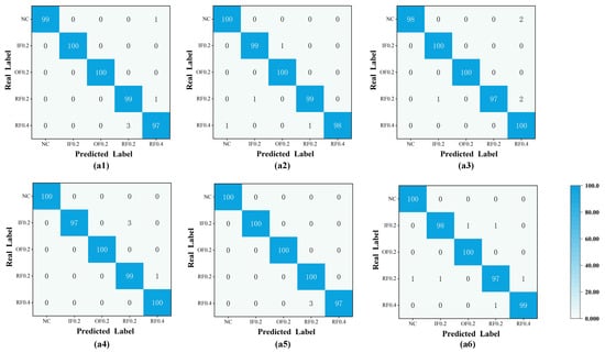
Figure 11. Confusion matrices of the PM across six tasks (A1–A6). (a1) Result from PM on task A1. (a2) Result from PM on task A2. (a3) Result from PM on task A3. (a4) Result from PM on task A4. (a5) Result from PM on task A5. (a6) Result from PM on task A6.

Comprehensive experimental evidence confirms that the proposed framework delivers reliable diagnostic performance and strong generalization across multiple transfer scenarios. Its effectiveness arises from the integration of time–frequency feature fusion and dual-domain distance metrics, enabling precise distinctions among subtle fault variations while preserving stability in complex environments. Time–frequency fusion compensates for the incompleteness of single-domain descriptions and provides richer representations. The residual attention mechanism preserves critical local details and reinforces the ability to detect fault-related patterns. The dual-domain distance metric assesses the discrepancy between operating conditions more accurately and increases diagnostic reliability. These components collectively establish a dependable foundation for intelligent fault detection under highly variable mechanical environments.

4.2.5. Computational Complexity Analysis

To further evaluate the feasibility of deploying the proposed PM in practical industrial monitoring environments, a detailed computational analysis is conducted. The assessment includes parameter scale, floating-point operations, training overhead, inference latency, and memory usage. Table 4 provides a structured summary of the main results.

Table 4. Computational complexity overview of the PM.

Metric	PM Value (Approx.)	Interpretation
Parameter count	≈9–11 M	Far smaller than ViT-Base (≈86 M), enabling lightweight deployment
FLOPs	≈1.7–2.3 GFLOPs	Reduced computation due to 6-layer × 4-head design
Training time per epoch	≈15–25 s (RTX 4060)	Faster convergence with moderate hardware
Inference latency	≈3–5 ms/sample	Meets real-time industrial monitoring requirements
Peak memory usage	≈2–2.5 GB	Suitable for mid-range GPUs and edge devices

These results indicate that the PM maintains an effective balance between representational capacity and computational efficiency. The constrained encoder depth and reduced attention-head arrangement significantly lower the overall computational cost. At the same time, the hybrid time–frequency fusion preserves strong discriminative ability. Overall, the PM can support real-time fault diagnosis tasks under limited hardware resources and meet the latency constraints required in industrial scenarios.

4.3. Experiment B: Fault Diagnosis Under Gears Data

4.3.1. Data Description of Experiment A

A series of transfer experiments across multiple velocities is performed to investigate cross-domain fault detection under varying workloads. The experimental conditions are summarized in Table 3. Experiment B focuses on gears operating under different loads. Data are collected at 1000 RPM and divided into six subtasks, B1 through B6, as listed in Table 5. The same neural architecture is used throughout the experiments, and the source and target domains contain equal sample sizes to maintain consistency with the setup of Experiment A.

Table 5. Description of operating conditions for each scenario in Experiment B.

Transfer Task	Source Domain	Target Domain
	Fluctuation Load (N)	Fluctuation Load (N)
B1	0~0.2 A	0~0.35 A
B2	0~0.2 A	0~0.5 A
B3	0~0.35 A	0~0.2 A
B4	0~0.35 A	0~0.5 A
B5	0~0.5 A	0~0.2 A
B6	0~0.5 A	0~0.35 A

4.3.2. Comparative Evaluation of Experiment B

The same statistical protocol used in Section 4.2 is applied here. Each experiment is repeated ten times, and the standard deviations are recorded in Table 4. Paired t-tests between the PM and each comparison approach yield p < 0.01. A one-way ANOVA across all methods results in p < 0.001. These statistics confirm that the performance differences observed in Experiment B are significant and align with the trends established in Experiment A.

In Experiment B, the network configuration and hardware environment are identical to those used in Experiment A. The differences stem from the experimental subjects and transfer conditions. These factors may influence certain computational metrics such as parameter scale, FLOPs, training time per epoch, and inference latency. However, the overall results remain within the range reported in Experiment A, and the detailed metrics can be found in Section 4.2.5.

4.3.3. Experimental Results of Experiment B

Table 6 and Figure 12 show that the PM achieves the highest accuracy across the six transfer tasks. The values for B1, B3, and B6 reach 99.19%, 99.40%, and 99.14%, respectively. Although CM3, CM4, CM5, and CM6 attain accuracies above 96%, the PM demonstrates smaller standard deviations and stronger robustness. These results confirm that integrating hybrid time–frequency representations, residual attention, and multiple domain-distance metrics enhances cross-domain learning and improves diagnostic stability under fluctuating loads.

Table 6. Overview of diagnostic findings of Experiment B.

Accuracy	CM1	CM2	CM3	CM4	CM5	CM6	PM
B1	87.41 ± 4.53	93.96 ± 3.83	96.60 ± 1.85	97.82 ± 1.81	96.12 ± 2.05	97.38 ± 1.75	99.19 ± 0.50
B2	87.35 ± 4.28	92.97 ± 3.72	95.07 ± 2.75	95.93 ± 2.18	97.05 ± 1.89	97.62 ± 1.33	98.80 ± 0.71
B3	90.60 ± 3.84	93.95 ± 2.98	96.89 ± 2.09	97.36 ± 1.55	97.22 ± 2.10	98.05 ± 1.57	99.40 ± 0.38
B4	89.72 ± 3.64	94.46 ± 3.11	96.75 ± 1.65	96.97 ± 1.89	97.75 ± 1.92	98.19 ± 1.41	98.93 ± 0.47
B5	87.76 ± 4.66	93.11 ± 3.47	94.80 ± 2.06	95.48 ± 2.53	96.85 ± 1.78	97.24 ± 1.82	99.16 ± 0.69
B6	87.14 ± 3.47	95.17 ± 2.76	96.51 ± 2.14	97.72 ± 1.67	97.18 ± 1.60	97.46 ± 1.08	99.14 ± 0.55

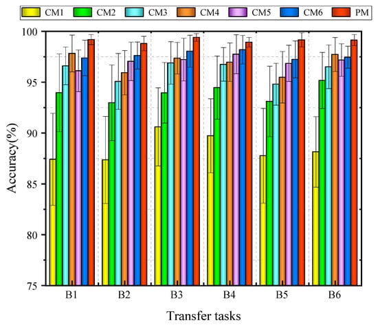
Figure 12. Accuracy comparison of methods under Experiment B.

Figure 13 presents violin plots that display accuracy distributions for the six methods. The PM shows a compact distribution with a high median accuracy and a narrow spread, indicating strong stability. In contrast, CM1 through CM6 exhibit wider distributions and lower extremes, demonstrating higher variability and reduced reliability. The concentrated distribution and short error bars of the PM confirm its consistent behavior across all transfer tasks.

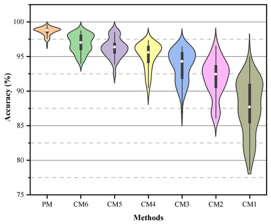
Figure 13. Visualizations of accuracy spread across the five techniques.

To further examine transfer capability, the t-SNE algorithm is applied for visualization and analysis. Figure 14 shows that the PM forms tight clusters within each fault category across all six transfer tasks, despite the differences between the source and target domains. This observation confirms accurate fault identification and stable performance under domain shifts. The visualization also reveals cohesive sample dispersion and clear category boundaries, further validating the strong cross-domain generalization provided by the PM.

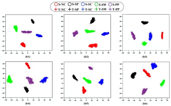
Figure 14. Dimensionality reduction visualization of the PM across tasks B1–B6. (b1) Visualization from PM on task B1. (b2) Visualization from PM on task B2. (b3) Visualization from PM on task B3. (b4) Visualization from PM on task B4. (b5) Visualization from PM on task B5. (b6) Visualization from PM on task B6.

Figure 15 presents the confusion matrix summarizing classification performance for the five fault categories. The PM achieves the most stable and accurate results. CM1 shows more than 20% misclassification in two categories and demonstrates limited robustness. The remaining comparison methods reach high accuracy in some categories but produce inconsistent outcomes in others. In contrast, the PM maintains accuracy above 97% in all categories, with an average value close to 99%. These findings confirm that the PM delivers reliable fault discrimination and strong cross-domain generalization across fluctuating operating conditions.

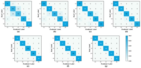
Figure 15. Comparison of confusion metrics of the transfer task B2 methodologies. (a) Confusion matrix for CM1. (b) Confusion matrix for CM2. (c) Confusion matrix for CM3. (d) Confusion matrix for CM4. (e) Confusion matrix for CM5. (f) Confusion matrix for CM6. (g) Confusion matrix for PM.

5. Conclusions

This study presents a fault diagnosis framework that integrates time–frequency fusion, residual attention, and a hybrid dual-domain metric to alleviate feature over-globalization under fluctuating operating conditions. Complementary time–frequency information increases representation diversity, and residual attention strengthens the ability of the network to extract fault-relevant cues across different layers. The hybrid metric formed by Wasserstein distance and MMD enhances domain alignment across varying environments, resulting in a more reliable feature transfer process. The proposed approach delivers consistent diagnostic performance across a wide range of speeds and loads. Beyond accuracy, the framework maintains favorable computational characteristics. The encoder depth is controlled to avoid excessive parameter growth, and the number of attention heads remains modest to reduce computational overhead. Multi-scale fusion and residual attention contribute only to linear complexity, allowing the model to retain strong expressive capacity without imposing high hardware requirements. The overall parameter count, FLOPs, memory consumption, and inference latency remain at a level appropriate for mid-range GPUs and embedded monitoring platforms, indicating practical feasibility for real-time industrial applications.

Although the method shows strong adaptability across diverse transfer conditions, two scenarios may require additional attention. Highly irregular spectral distributions can reduce the effectiveness of the current multi-scale segmentation strategy, and severe domain imbalance may affect dual-domain metric sensitivity when only a limited number of target samples are available. These considerations define the boundaries within which the present framework operates most effectively. Future work will extend the design to address these scenarios. Multi-sensor fusion and adaptive segmentation strategies may improve performance when the spectral distribution becomes irregular. Techniques for dynamic sample reweighting and domain-aware feature calibration may alleviate the influence of domain imbalance. Further efforts toward lightweight architectures, hardware-adaptive acceleration, and streaming data processing will support deployment in real-time industrial environments with stricter latency constraints.

References

- Lu, J.; Wu, W.; Huang, X.; Yin, Q.; Yang, K.; Li, S. A modified active learning intelligent fault diagnosis method for rolling bearings with unbalanced samples. Adv. Eng. Inform. 2024, 60, 102397. [Google Scholar] [CrossRef]
- Xu, X.; Ou, X.; Ge, L.; Qiao, Z.; Shi, P. Simulated Data-Assisted Fault Diagnosis Framework with Dual-Path Feature Fusion for Rolling Element Bearings under Incomplete Data. IEEE Trans. Instrum. Meas. 2025, 74, 3542617. [Google Scholar] [CrossRef]
- Wang, J.; Zhang, Z.; Liu, Z.; Han, B.; Bao, H.; Ji, S. Digital twin aided adversarial transfer learning method for domain adaptation fault diagnosis. Reliab. Eng. Syst. Saf. 2023, 234, 109152. [Google Scholar] [CrossRef]
- Xu, X.; Yang, X.; He, C.; Shi, P.; Hua, C. Adversarial Domain Adaptation Model Based on LDTW for Extreme Partial Transfer Fault Diagnosis of Rotating Machines. IEEE Trans. Instrum. Meas. 2024, 73, 3538811. [Google Scholar] [CrossRef]
- Jiang, X.; Song, Q.; Wang, H.; Du, G.; Guo, J.; Shen, C.; Zhu, Z. Central frequency mode decomposition and its applications to the fault diagnosis of rotating machines. Mech. Mach. Theory 2022, 174, 104919. [Google Scholar] [CrossRef]
- Almutairi, K.; Sinha, J. A Comprehensive 3-Steps Methodology for Vibration-Based Fault Detection, Diagnosis and Localization in Rotating Machines. J. Dyn. Monit. Diagn. 2024, 3, 49–58. [Google Scholar] [CrossRef]
- Lu, J.; Qian, W.; Li, S.; Cui, R. Enhanced K-Nearest Neighbor for Intelligent Fault Diagnosis of Rotating Machinery. Appl. Sci. 2021, 11, 919. [Google Scholar] [CrossRef]
- Jiang, X.; Wang, J.; Shen, C.; Shi, J.; Huang, W.; Zhu, Z.; Wang, Q. An adaptive and efficient variational mode decomposition and its application for bearing fault diagnosis. Struct. Health Monit. 2021, 20, 2708–2725. [Google Scholar] [CrossRef]
- Wu, Y.; Song, J.; Wu, X.; Wang, X.; Lu, S. Fault Diagnosis of Linear Guide Rails Based on SSTG Combined with CA-DenseNet. J. Dyn. Monit. Diagn. 2024, 3, 1–10. [Google Scholar] [CrossRef]
- Shao, H.; Lai, Y.; Liu, H.; Wang, J.; Liu, B. LSFConvformer: A lightweight method for mechanical fault diagnosis under small samples and variable speeds with time-frequency fusion. Mech. Syst. Signal Process. 2025, 236, 113016. [Google Scholar] [CrossRef]
- Huang, T.; Zhang, Q.; Tang, X.; Zhao, S.; Lu, X. A novel fault diagnosis method based on CNN and LSTM and its application in fault diagnosis for complex systems. Artif. Intell. Rev. 2022, 55, 1289–1315. [Google Scholar] [CrossRef]
- Jiang, X.; Li, X.; Wang, Q.; Song, Q.; Liu, J.; Zhu, Z. Multi-sensor data fusion-enabled semi-supervised optimal temperature-guided PCL framework for machinery fault diagnosis. Inf. Fusion 2024, 101, 102005. [Google Scholar] [CrossRef]
- Chen, Z.; Gryllias, K.; Li, W. Mechanical fault diagnosis using Convolutional Neural Networks and Extreme Learning Machine. Mech. Syst. Signal Process. 2019, 133, 106272. [Google Scholar] [CrossRef]
- Hu, Z.; Han, T.; Bian, J.; Wang, Z.; Cheng, L.; Zhang, W.; Kong, X. A deep feature extraction approach for bearing fault diagnosis based on multi-scale convolutional autoencoder and generative adversarial networks. Meas. Sci. Technol. 2022, 33, 065013. [Google Scholar] [CrossRef]
- Li, X.; Xiao, S.; Zhang, F.; Huang, J.; Xie, Z.; Kong, X. A fault diagnosis method with AT-ICNN based on a hybrid attention mechanism and improved convolutional layers. Appl. Acoust. 2024, 225, 110191. [Google Scholar] [CrossRef]
- Wu, Z.; Jiang, H.; Zhu, H.; Wang, X. A knowledge dynamic matching unit-guided multi-source domain adaptation network with attention mechanism for rolling bearing fault diagnosis. Mech. Syst. Signal Process. 2023, 189, 110098. [Google Scholar] [CrossRef]
- Qian, Q.; Qin, Y.; Luo, J.; Wang, Y.; Wu, F. Deep discriminative transfer learning network for cross-machine fault diagnosis. Mech. Syst. Signal Process. 2023, 186, 109884. [Google Scholar] [CrossRef]
- Zhao, D.; Liu, S.; Zhang, T.; Zhang, H.; Miao, Z. Subdomain adaptation capsule network for unsupervised mechanical fault diagnosis. Inf. Sci. 2022, 611, 301–316. [Google Scholar] [CrossRef]
- Li, J.; Chen, X.; He, Z. Multi-stable stochastic resonance and its application research on mechanical fault diagnosis. J. Sound Vib. 2013, 332, 5999–6015. [Google Scholar] [CrossRef]
- Xu, Y.; Chen, Y.; Zhang, H.; Feng, K.; Wang, Y.; Yang, C.; Ni, Q. Global contextual feature aggregation networks with multiscale attention mechanism for mechanical fault diagnosis under non-stationary conditions. Mech. Syst. Signal Process. 2023, 203, 110724. [Google Scholar] [CrossRef]
- He, K.; Zhang, X.; Ren, S.; Sun, J. Deep residual learning for image recognition. In Proceedings of the IEEE Conference on Computer Vision and Pattern Recognition, Las Vegas, NV, USA, 27–30 June 2016; pp. 770–778. [Google Scholar]
- Bao, H.; Kong, L.; Lu, L.; Wang, J.; Zhang, Z.; Han, B. A new multi-layer adaptation cross-domain model for bearing fault diagnosis under different operating conditions. Meas. Sci. Technol. 2024, 35, 106116. [Google Scholar] [CrossRef]
- Xing, S.; Wang, J.; Han, B.; Zhang, Z.; Jiang, X.; Ma, H.; Zhang, X.; Shao, H. Dual-domain Signal Fusion Adversarial Network Based Vision Transformer for Cross-domain Fault Diagnosis. In Proceedings of the 2023 Global Reliability and Prognostics and Health Management Conference (PHM-Hangzhou), Hangzhou, China, 12–15 October 2023; IEEE: New York, NY, USA; pp. 1–5. [Google Scholar]
- Liu, Z.; Lin, Y.; Cao, Y.; Hu, H.; Wei, Y.; Zhang, Z.; Lin, S.; Guo, B. Swin transformer: Hierarchical vision transformer using shifted windows. In Proceedings of the IEEE/CVF International Conference on Computer Vision 2021, Montreal, QC, Canada, 10–17 October 2021; pp. 9992–10002. [Google Scholar]
- Chen, J.; Kao, S.-H.; He, H.; Zhuo, W.; Wen, S.; Lee, C.-H.; Chan, S.-H.G. Run, don’t walk: Chasing higher FLOPS for faster neural networks. In Proceedings of the IEEE/CVF Conference on Computer Vision and Pattern Recognition 2023, Vancouver, BC, Canada, 17–24 June 2023; pp. 12021–12031. [Google Scholar]
- Li, X.; Yu, T.; Wang, X.; Li, D.; Xie, Z.; Kong, X. Fusing joint distribution and adversarial networks: A new transfer learning method for intelligent fault diagnosis. Appl. Acoust. 2024, 216, 109767. [Google Scholar] [CrossRef]
- Zheng, B.; Huang, J.; Ma, X.; Zhang, X.; Zhang, Q. An unsupervised transfer learning method based on SOCNN and FBNN and its application on bearing fault diagnosis. Mech. Syst. Signal Process. 2024, 208, 111047. [Google Scholar] [CrossRef]
- Van der Maaten, L.; Hinton, G. Visualizing data using t-SNE. J. Mach. Learn. Res. 2008, 9, 2579–2605. [Google Scholar]
Disclaimer/Publisher’s Note: The statements, opinions and data contained in all publications are solely those of the individual author(s) and contributor(s) and not of MDPI and/or the editor(s). MDPI and/or the editor(s) disclaim responsibility for any injury to people or property resulting from any ideas, methods, instructions or products referred to in the content. |
© 2025 by the authors. Licensee MDPI, Basel, Switzerland. This article is an open access article distributed under the terms and conditions of the Creative Commons Attribution (CC BY) license (https://creativecommons.org/licenses/by/4.0/).