Passable Region Identification Method for Autonomous Mobile Robots Operating in Underground Coal Mine

Abstract

Aiming at the problems of insufficient environmental perception capability of autonomous mobile robots and low multi-modal data fusion efficiency in the complex underground coal mine environment featuring low illumination, high dust, and dynamic obstacles, a reliable passable region identification method for autonomous mobile robots operating in underground coal mine is proposed in this paper. Through the spatial synchronous installation strategy of dual 4D millimeter-wave radars and dynamic coordinate system registration technology, it increases point cloud density and effectively enhances the spatial characterization of roadway structures and obstacles. Combining the characteristics of infrared thermal imaging and the penetration advantage of millimeter-wave radar, a multi-modal data complementary mechanism based on decision-level fusion is proposed to solve the perceptual blind zones of single sensors in extreme environments. Integrated with lightweight model optimization and system integration technology, an intelligent environmental perception system adaptable to harsh working conditions is constructed. The experiments were carried out in the simulated tunnel. The experiments were carried out in the simulated tunnel. The experimental results indicate that the robot can utilize the data collected by the infrared camera and the radar to identify the specific distance to obstacles, and can smoothly achieve the recognition and marking of passable areas.

1. Introduction

The research on passable area recognition technology for autonomous mobile robots in coal mines focuses on obstacle recognition within the motion scene of underground electromechanical equipment. Object detection [1] and object tracking [2], as core tasks in the field of computer vision, are highly relevant. Object detection aims to identify objects in images and determine their locations, while object tracking continuously locates and tracks specific targets in video sequences. The two tasks overlap and complement each other technically, and are widely applied in complex scenarios such as autonomous driving and underground coal mines.

In terms of object detection technology, its development has evolved from single-sensor approaches to multi-sensor fusion. In 2012, Kellner et al. [3] improved the DBSCAN algorithm and proposed a grid-based clustering method to address the uneven sampling density of millimeter-wave radar point clouds. In 2017, Mousavian et al. [4] proposed 3DBoxEstimation, which leverages 2D and 3D bounding box constraints to improve camera detection accuracy, while Prabhakara et al. [5] designed a high-performance radar system to generate denser point cloud data. In 2018, Chen et al. [6] introduced the Mono3D algorithm, which uses monocular cameras and energy minimization with handcrafted features for 3D object detection. In 2019, Zhang et al. proposed an elliptical density clustering algorithm for millimeter-wave radar, while Scheiner et al. employed an LSTM classifier for object classification [7,8]. In 2023, Liu et al. [9] presented a multi-perception feature-based detection method that improved both speed and robustness. Regarding multi-sensor fusion, Nabati, Felix, Chadwick, and others [10,11,12,13] explored radar-vision fusion techniques.

In infrared target tracking, development has gone through three stages: generative methods, correlation filter-based methods, and deep learning methods. Generative algorithms achieve tracking by searching for regions most similar to the target model, with representative methods including mean shift, particle filtering, and Kalman filtering, typically relying on templates or sparse representations. Correlation filter-based methods adopt a discriminative approach, training classifiers to localize targets. For example, Henriques et al. proposed the CSK algorithm [14], introducing kernel tricks and cyclic sampling to improve accuracy. Zhang et al. introduced the STC algorithm [15], which emphasizes contextual relationships. In 2014, Danelljan et al. proposed DSST [16], which used a 3D filter to handle scale variations, and later optimized it into fDSST [17] in 2017 to enhance speed and accuracy. Li and Zhu presented the SAMF algorithm [18] to improve scale adaptability. In deep learning-based methods, Bertinetto et al. proposed Siamese-FC [19] in 2016, employing a Siamese network to balance accuracy and speed. In 2019, Li et al. developed Siamese-RPN++, integrating deep semantic information [20]. In 2021, Chen et al. designed an attention-based feature fusion network [21].

For passable area detection, Nie Yiming first introduced the concept of passability to describe whether a robot can traverse a specific region, while Manduchi and Castano [22] defined it in terms of affordance for traversal. For mobile robots, two types of potential hazards may render an area impassable: geometric hazards, caused by physical features that block passage, and non-geometric hazards, such as density or viscosity of terrain that hinder or completely stop motion. The key to passable area recognition lies in rapid obstacle detection and terrain classification. In 2015, Jiang Jianfei et al. applied an improved Euclidean clustering algorithm for real-time obstacle detection, extracting passable areas based on inter-point spacing, angular differences, and clustering, but struggled with irregular obstacles along roadsides. In 2018, Duan Jianmin et al. improved the COBWEB algorithm for Euclidean clustering of curbs and used least squares fitting for left and right curb modeling. In 2019, Shen Hua et al. improved the activation function of a fully convolutional network, developing M-FCN for road recognition in SAR images to mitigate information loss, though still at an exploratory stage. In 2024, Dai Bo et al. proposed a mine road passable area recognition method using concentric circle modeling, spatial connectivity filtering, and temporal stability analysis. The AlexNet proposed by Krizhevsky et al. [23] greatly advanced CNN applications in computer vision. PointNet and PointNet++ by Qi et al. [24] laid the foundation for deep learning in point cloud segmentation, though their performance is limited in large-scale outdoor point clouds. Velas et al. proposed a method to project 3D point clouds into 2D for CNN-based segmentation, training relatively shallow networks on manually labeled datasets to separate ground points.

However, the underground coal mine environment is complex, with factors such as low illumination, point light sources, dust, and water mist severely limiting the scene perception accuracy of sensors and the stability of multimodal fusion, thereby resulting in low travel efficiency of autonomous mobile robots in the mine. Therefore, this research addresses challenges in underground coal mine tunnels, such as insufficient environmental perception capability of autonomous mobile robots and low efficiency in multi-modal data fusion, by studying methods for passable area and obstacle recognition with the infrared thermal imagers and 4D millimeter-wave radars, which are insensitive to interference elements. First, for multi-sensor data processing, a dual-radar strategy is designed to densify point clouds and mitigate sparsity in single-radar setups. Point cloud data is then denoised and optimized, while noisy infrared images are enhanced to provide high-quality data for subsequent object detection. Second, in obstacle detection, the You Only Look Once (YOLO) series has been improved through channel optimization, the addition of new modules, and adjustments to the loss function. Using the installation positions of millimeter-wave radar and infrared cameras, coordinate transformations are performed to align the two sensor coordinate systems with the mobile robot frame, ensuring spatial synchronization and scene consistency to improve detection accuracy. The improved YOLO algorithm is applied to recognize infrared targets in tunnels, while clustering algorithms determine the positions of obstacles in the point cloud and compute their distances from the radar origin, thereby defining passable areas. An experimental platform for passable area recognition, based on infrared cameras and millimeter-wave radar, has been built, with a system architecture designed to determine passable regions. The YOLO detection network is trained using infrared datasets collected in tunnels. The main contributions of the article are concluded as follows:

(1)

By adopting infrared thermal imaging and 4D radar distance measurement technologies, the core issue of the underground scene perception system in coal mines, which is severely affected by the complex underground scenarios, has been solved.

(2)

The passable region reliable identification method for autonomous mobile robots operating in underground coal mine with the infrared thermal imaging and 4D radar distance measurement technologies.

(3)

Simulation experiments and industrial tests were carried out, which proved the applicability and reliability of the proposed passable region reliable identification method.

The paper is organized as follows. Data preprocessing of the information obtained from the infrared camera and the 4D millimeter-wave radar is described in Section 2. In Section 3, an improved YOLOv5 algorithm is introduced for object detection. Section 4 presents simulation experiments conducted using the constructed dataset. The experimental validation in Section 5 is carried out with a mobile robot equipped with an infrared camera and a 4D millimeter-wave radar in the simulated tunnel. Conclusion and outlook are provided in Section 6.

2. Processing of Data

In underground harsh environments, the infrared images captured by cameras are significantly affected by dust and water mist, resulting in substantial noise within the imaging process. Such noise interferes with the extraction of target information, thereby reducing the accuracy and reliability of infrared target recognition. Consequently, the raw infrared image data cannot be directly applied to high-precision target detection and passable area identification, necessitating further data processing.

To address the denoising problem of infrared images, this study proposes a hybrid denoising algorithm that not only suppresses noise but also enhances edge details of infrared targets, thereby improving overall image quality. Meanwhile, considering the low density of millimeter-wave radar point cloud data, a combined filtering strategy is employed to refine the point clouds, improving both accuracy and reliability. Through these preprocessing methods, the proposed approach ensures high-quality data for passable area recognition and obstacle detection of autonomous mobile equipment in coal mines, thereby enhancing the accuracy and robustness of the recognition system.

2.1. Infrared Image Processing

2.1.1. Hybrid Denoising Algorithm

Non-Local Means (NLM) filtering [25] is a denoising algorithm based on image self-similarity. The core idea of NLM is to exploit the similarity of non-local regions within an image to remove noise. Compared with traditional local filtering methods, NLM can better preserve image details and structural information, particularly demonstrating superior performance in handling Gaussian noise. Its fundamental formula is expressed as:

$$\widehat{I}(x)={\displaystyle \frac{1}{C\left(x\right)}}{\displaystyle \sum _{y\hspace{0.17em}\in \hspace{0.17em}\Omega }\omega (x,y)I\left(y\right)}$$

(1)

Here, $\widehat{I}(x)$ is the denoised value of pixel $x$; $I\left(y\right)$ is the value of pixel $y$ in the original image; $\omega (x,y)$ is the weight that measures the similarity between pixels $x$ and $y$; $C\left(x\right)$ is the normalization factor, defined as $C(x)={\displaystyle \sum _{y\hspace{0.17em}\in \hspace{0.17em}\Omega }\omega (x,y)}$; and $\Omega$ denotes the entire pixel domain of the image.

The weight $\omega (x,y)$ is calculated based on the similarity of the neighborhoods of pixels $x$ and $y$, as follows:

$$\omega (x,y)=\exp \left(-{\displaystyle \frac{\Vert I(N_x)-I\left(N_y\right){\Vert }_2^2}{h^2}}\right)$$

(2)

where $N_x$ and $N_y$ represent the neighborhoods centered at pixels $x$ and $y$ respectively; $\Vert I\left(N_x\right)-I\left(N_y\right){\Vert }_2^2$ denotes the Euclidean distance between the two neighborhoods, which measures their similarity; and $h$ is a parameter controlling the decay rate of the weights, usually related to the noise level.

To mitigate the potential oversmoothing effect of NLM denoising, this study further applies an edge detection algorithm based on the Sobel operator. The key idea of this method is to compute the gradient value of each pixel through convolution operations, thereby detecting edges in the image. A gradient is a vector that indicates both the direction and the rate of the fastest intensity change in the image. The Sobel operator employs two convolution kernels to calculate gradients in the horizontal and vertical directions. By combining the gradient values in these two directions, both the gradient magnitude and orientation of each pixel can be obtained, enabling accurate edge localization.

To further improve processing performance, this paper integrates the NLM denoising algorithm with an enhanced Sobel edge detection algorithm to construct an image processing system. The specific process is as follows:

First, the original image is subjected to aggressive NLM smoothing to filter out more noise, although this results in a significant loss of global information. Subsequently, clear target edge information is obtained through contrast enhancement and the Sobel edge extraction method. Meanwhile, after applying standard NLM denoising and contrast enhancement to the original image, the edges extracted from the aggressive smoothing path are weighted and fused with the optimized image from the standard denoising path. The fused result then undergoes mild NLM denoising to produce the final denoised and enhanced image.

Given the characteristics of infrared images, such as uniformly distributed noise and low contrast between targets and the background, the hybrid denoising and enhancement algorithm proposed in this paper employs strategies including parallel processing paths, contrast enhancement, and weighted fusion. This structure skillfully integrates the advantages of NLM denoising and Sobel edge enhancement, aiming to reconcile the conflict between noise removal and edge preservation. The rationality and advantages of this architecture are theoretically analyzed as follows:

(1)

Complementarity of Parallel Processing Paths

The algorithm adopts two parallel paths: one is the aggressive NLM smoothing path, which strongly suppresses noise to provide a cleaner image basis for subsequent edge extraction, thereby avoiding interference from noise in Sobel operator-based edge detection; the other is the standard NLM denoising path, which removes most of the noise while preserving image details as much as possible. This parallel design theoretically achieves a balance between noise suppression and detail preservation, providing complementary sources of information for subsequent fusion.

(2)

Necessity of Contrast Enhancement

Due to the low contrast of the original infrared images, direct edge detection yields limited results. Therefore, introducing contrast enhancement in both paths theoretically amplifies the grayscale differences between targets and the background, thereby improving the sensitivity and accuracy of the Sobel operator in detecting target edges and reducing the loss of edge information.

(3)

Optimization Mechanism of Weighted Fusion

By performing weighted fusion between the precise edges extracted from the aggressive smoothing path and the detail-preserved image from the standard denoising path, the algorithm theoretically combines the advantages of both. This results in enhanced edge features of target objects while maintaining the overall structure and details of the image. This fusion mechanism optimizes both the visual quality and informational completeness of the image.

(4)

Refinement Role of Mild Denoising

The final step of mild NLM denoising theoretically acts as a “fine-tuning” process. It further suppresses any residual weak noise without damaging the details of the fused image, ensuring the purity of the final output.

2.1.2. Algorithm Test

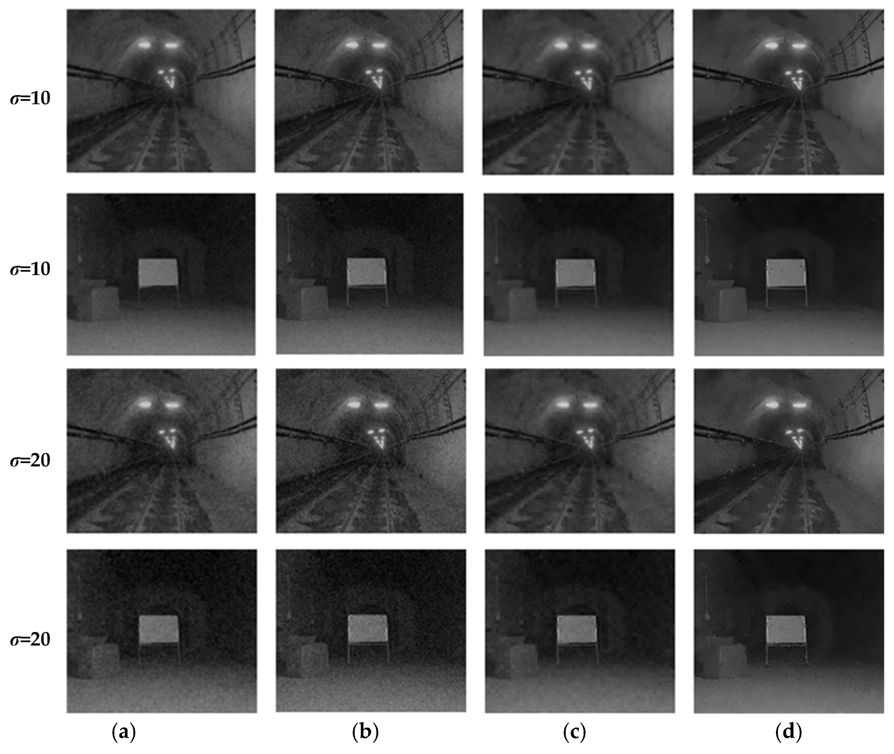
To verify the performance of the proposed hybrid algorithm, the optimized method in this paper is compared with traditional denoising approaches such as mean filtering, median filtering, and wavelet denoising. In this section, the image of the empty tunnel (1st and 3rd lines in Figure 1) and the image of the tunnel with an obstacle (2nd and 4th lines in Figure 1) are selected as the base images, which are used as the target images for the display of denoising effects in Figure 1. To verify the effectiveness of the proposed algorithm, the Gaussian noise with intensities of 10 and 20 are added, respectively, to the original tunnel images.

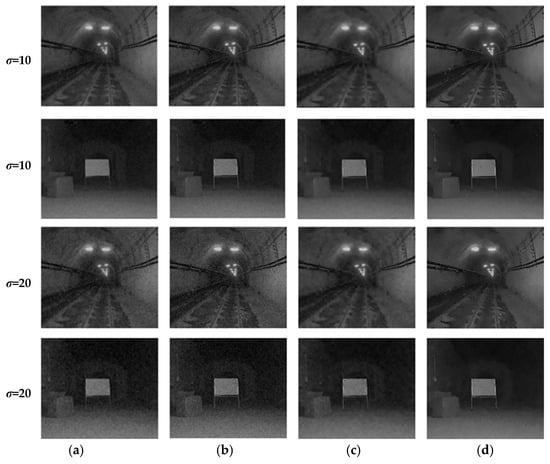
Figure 1. Comparison of denoising results. (a) Median filtering; (b) Mean filtering; (c) Wavelet denoising; (d) Non-Local Means filtering.

As shown in Figure 1, median filtering leads to severe loss of image details and unsatisfactory denoising performance. Mean filtering provides good detail preservation, but the denoising effect shows no significant improvement. In wavelet denoising, noise is greatly suppressed, but image details are heavily lost, resulting in a deterioration of overall image quality. In contrast, the Non-Local Means (NLM) filtering adopted in this study not only effectively removes Gaussian noise but also achieves maximum preservation of image details.

To further evaluate the performance of the selected method in this study, the denoising results are assessed using three metrics: Peak Signal-to-Noise Ratio (PSNR), Structural Similarity Index (SSIM), and Mean Square Error (MSE). The outcomes are presented in Table 1 and Table 2.

Table 1. Comparison of Denoising Image Evaluation Standards for Empty Tunnel Image.

Empty Tunnel		PSNR	SSIM	MSE
σ = 10	Median filtering	31.67	0.74	44.32
	Mean filtering	31.15	0.71	49.83
	Wavelet denoising	30.98	0.68	51.93
	Non-Local Means filtering	32.41	0.81	37.33
σ = 20	Median filtering	29.75	0.56	68.87
	Mean filtering	29.35	0.49	75.51
	Wavelet denoising	29.14	0.39	79.32
	Non-Local Means filtering	30.19	0.58	62.29

Table 2. Comparison of obs Denoising Image Evaluation Standards for Obstacle Tunnel Image.

Empty Tunnel		PSNR	SSIM	MSE
σ = 10	Median filtering	31.83	0.72	42.67
	Mean filtering	31.28	0.69	48.48
	Wavelet denoising	31.22	0.66	49.15
	Non-Local Means filtering	32.76	0.80	34.43
σ = 20	Median filtering	29.85	0.52	67.31
	Mean filtering	29.35	0.47	75.60
	Wavelet denoising	29.29	0.41	76.52
	Non-Local Means filtering	30.49	0.64	58.11

Among these metrics, the PSNR quantifies the similarity between the denoised image and the original noise-free image, with higher values indicating better denoising performance. The SSIM assesses the resemblance in luminance, contrast, and structure between the denoised and original images, where values closer to 1 reflect superior results. The MSE calculates the pixel-wise difference between the denoised and original images, with lower values denoting more effective noise removal. As evidenced by the index in Table 1 and Table 2, the Non-Local Means (NLM) filtering method achieves the highest evaluation scores under both noise levels, demonstrating its noteworthy denoising effectiveness. This outcome lays a solid foundation for high-accuracy infrared target recognition in subsequent stages, while also enhancing the overall stability and robustness of the system.

2.2. Four-Dimensional Millimeter-Wave Radar Data Processing

2.2.1. Point Cloud Filtering Algorithm

The raw point cloud data obtained from 4D millimeter-wave radar cannot be directly used, since some points exhibit drift, while outliers and noisy points may also appear. These invalid points degrade the quality of the point cloud data and increase the difficulty of subsequent target detection. Therefore, before using the point cloud for target detection, denoising and filtering must be applied to remove as many invalid points as possible while preserving useful points, thereby improving the accuracy of target detection.

The noise in millimeter-wave radar point clouds is generally divided into large-scale noise and small-scale noise. Large-scale noise mainly originates from false point cloud regions formed by multiple reflections of tunnel walls and continuous static point cloud layers generated by ground reflections. Such noise is characterized by broad coverage and strong spatial continuity. Small-scale noise mainly consists of randomly distributed droplet reflection points caused by underground mist and dust, as well as random outliers introduced by radar hardware.

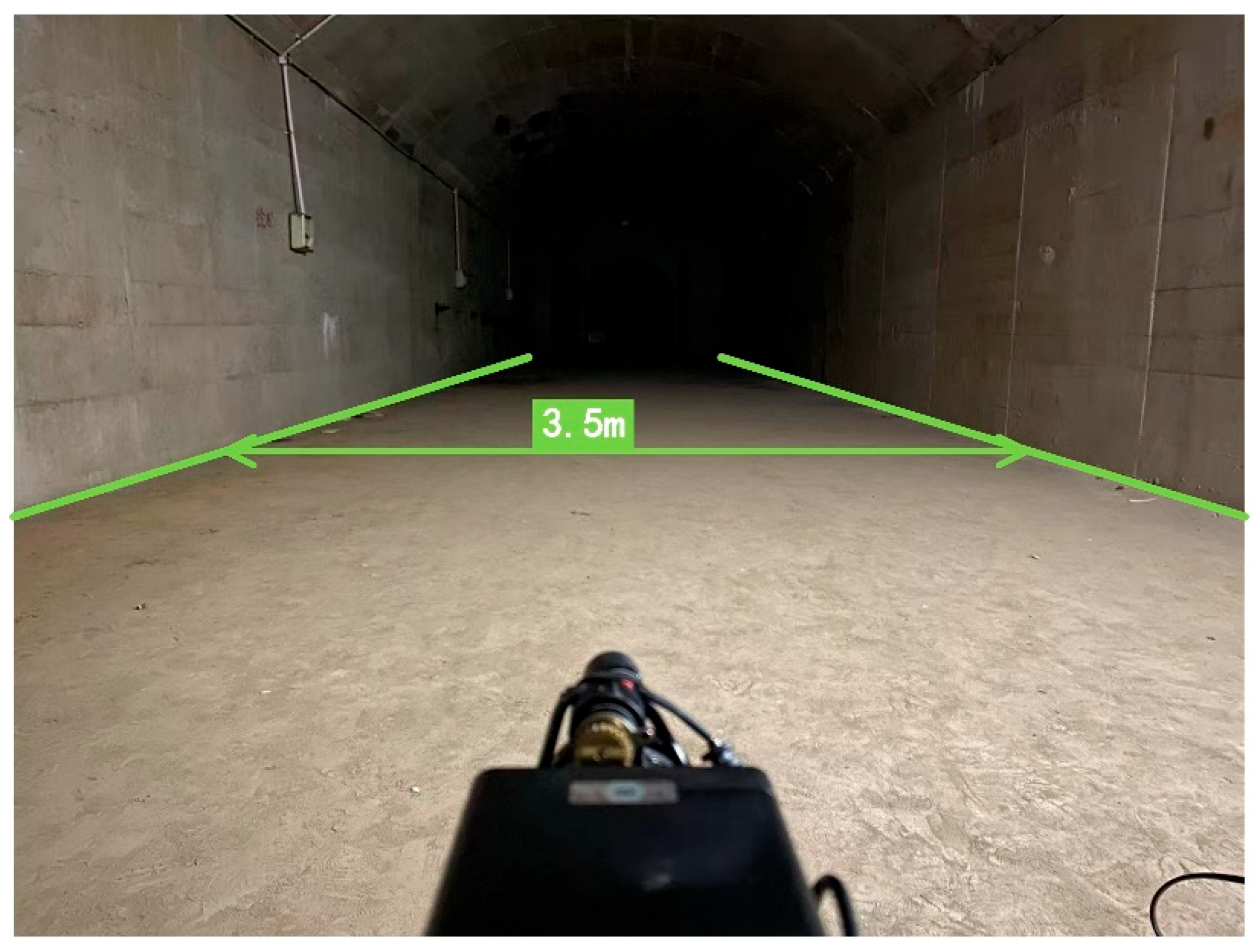
Based on the functional characteristics of different filtering algorithms, this study adopts three filtering methods: Pass-through filtering, Radius filtering, and Statistical filtering. For clarity, the explanation is provided based on the actual situation of the underground mine tunnels as shown in Figure 2.

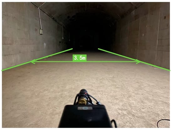
Figure 2. Original point cloud obtained by 4D millimeter-wave radar.

(1)

Pass-through filtering, used to crop tunnel boundaries and remove large-scale noise. The implementation is as follows:

For each point in the point cloud, if the following condition is met through Formula (3), keep the point; otherwise, remove it.

$$\begin{array}{l}{x}_{\min }\le x\le x_{\max }\\ y_{\min }\le y\le y_{\max }\\ z_{\min }\le z\le z_{\max }\end{array}$$

(3)

The reason for utilizing the Pass-through filtering is that the point clouds from millimeter-wave radars often contain noise and invalid points. Pass-through filtering can be used to remove these points: setting the Z-axis range can eliminate ground points, and setting the X and Y-axis ranges allows focusing on a specific area.

(2)

Radius filtering is applied to quickly eliminate isolated noise. The implementation is as follows:

Radius filtering can determine whether a point is a noise point based on its local density. If the number of neighboring points within a specified radius of a point is insufficient, it is considered a noise point and removed. For each point p_i in the point cloud, if the number of other points within a radius of r does not exceed the threshold k, then point p_i is removed.

(3)

Statistical filtering is employed to remove residual random outliers. The implementation is as follows:

Statistical filtering is based on the distribution characteristics of points in the point cloud. It assumes that there are differences in spatial distribution between noise points and valid points. By calculating the statistical characteristics of each point and its neighboring points, outliers and noise points can be identified and removed. For each point p_i in the point cloud, calculate the average distance between point p_i and its neighboring points:

$${\mu }_i={\displaystyle \frac{{\displaystyle \sum _{j=1}^n‖p_i-p_{ij}‖}}{n}}$$

(4)

where p_ij is the neighboring points and n is the total number of neighborhood points. Then, calculate the standard deviation of the distance:

$${\sigma }_i=\sqrt{{\displaystyle \frac{1}{n}}{\displaystyle \sum _{j=1}^n{(‖p_i-p_{ij}‖-{\mu }_i)}^2}}$$

(5)

Next, set the threshold T = μ ± ασ_i, where α is tunable parameter used to control the strictness of the filtering process. Finally, if the distance of a certain point exceeds the threshold range, it will be marked as a noise point and removed.

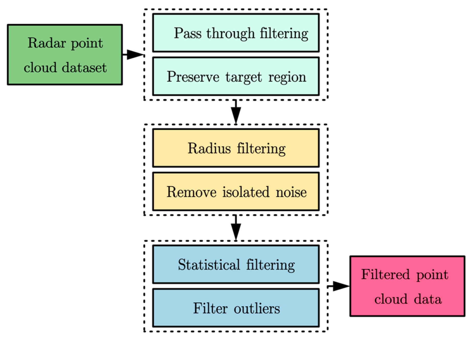
The filtering workflow is shown in Figure 3.

Figure 3. Filter flowchart.

2.2.2. Algorithm Test

In the simulation test, the point cloud of a bottle obstacle was selected as the test case. The raw point cloud contained a large amount of both large-scale and small-scale noise. Large-scale noise produced false tunnel boundaries inconsistent with the main tunnel structure, while small-scale noise included many locally sparse points, isolated points, and outliers near the obstacle surface.

First, pass-through filtering was applied to remove point cloud data outside the target range. Then, based on the result of pass-through filtering, radius filtering was applied to process sparse and isolated points, eliminating regions of low density. Finally, statistical filtering was adopted to remove outliers close to the tunnel structure, making both tunnel boundaries and obstacle contours more clearly visible. Ultimately, these steps provided high-quality data for subsequent traversable area recognition and obstacle detection. Figure 4 illustrates the comparison of the bottle obstacle point cloud before and after combined filtering.

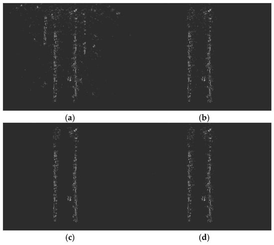
Figure 4. Comparison of point clouds before and after filtering. (a) Point cloud before filtering; (b) Point cloud after Pass-through filtering; (c) Point cloud after Radius filtering; (d) Point cloud after Statistical filtering.

To further verify the reliability of the optimized point cloud data, the following will compare the roadway data formed by the point cloud with the distance data of the actual tunnel boundaries. Since the accuracy of millimeter-wave radar is related to the distance, the tunnel is segmented for testing (each 5 m as one segment), in order to separately evaluate the accuracy of the point cloud in different distance segments. Table 3 shows the comparison of errors in average deviation, standard deviation and RMSE in different roadway segments.

Table 3. Error comparison of the roadway data formed by the point cloud with the distance data of the actual tunnel boundaries.

Segment Number	Distance Range	Mean Deviation	Standard Deviation	RMSE
1	0–5	0.22	0.16	0.27
2	5–10	0.26	0.18	0.30
3	10–15	0.28	0.21	0.33
4	15–20	0.31	0.23	0.36

It can be seen in Table 3, it can be seen that as the distance increases, the accuracy of the point cloud also continuously decreases. However, within the range of 0–20 m, the increase in error is relatively small and meets the requirements for obstacle detection in underground coal mines.

3. Object Detection Method

In the study of traversable area recognition in underground roadways, obstacle detection and classification are essential tasks. It is first necessary to promptly identify the type of obstacle in front of the mobile robot, providing a basis for operators to make further decisions. Subsequently, additional information such as the distance and size of the obstacle can be obtained using millimeter-wave radar. Considering the characteristics of the mobile robot’s working environment, high-performance devices often imply a larger volume, which is not suitable for underground deployment. Therefore, in this paper, the YOLOv5 model [26] is improved to achieve lightweight design, making it more suitable for use in underground environments. This ensures the real-time performance of traversable area recognition for mobile equipment in coal mine roadways.

3.1. YOLOv5 Model

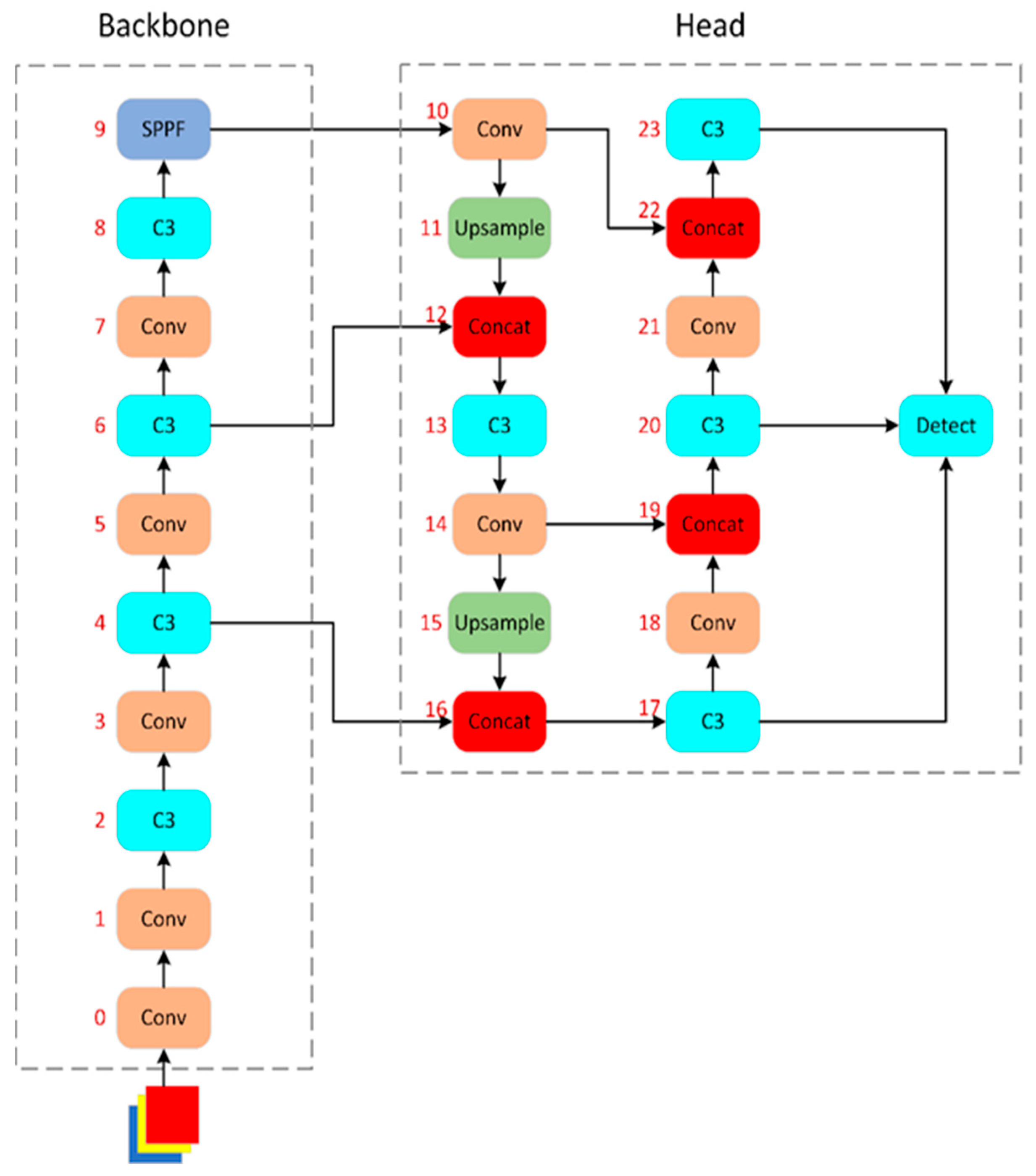
YOLOv5 adopts a modular design consisting of three main components: the Backbone, the Neck, and the Head, forming a workflow of feature extraction–feature fusion–object prediction (Figure 5). The Backbone uses CSPDarknet53 with Cross Stage Partial connections to extract multi-scale features efficiently. The Neck applies PANet to fuse features through top-down and bottom-up paths, integrating semantic and detail information for better multi-scale detection. The Head outputs bounding boxes, class confidence, and objectness scores based on fused features. This design optimizes feature extraction and fusion, enabling YOLOv5 to achieve a balance between speed and accuracy in real-time monitoring.

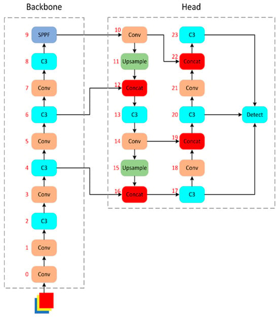
Figure 5. YOLOv5 network structure.

In the network structure and model configuration of Figure 5, only the Backbone and Head are explicitly defined, with the Neck omitted. This reflects a design choice in YOLOv5, where feature fusion and prediction are integrated into the Head instead of using a separate Neck. The Backbone, based on CSPDarknet53, serves as the core feature extractor. It improves upon Darknet53 with Cross Stage Partial (CSP) connections, reducing computation through channel splitting. The Backbone is built from stacked Conv and C3 modules, with its key parameters summarized in Table 4.

Table 4. Backbone key parameters.

Layer	Module Composition	Input Size	Output Size
Input	Focus/Conv	640 × 640 × 32	32
1	Conv + C3	320 × 320 × 64	64
2	Conv + C3 × 2	160 × 160 × 128	128
3	Conv + C3 × 3	80 × 80 × 256	256
4	Conv + C3 + SPP	40 × 40 × 512	512

In YOLOv5, the Backbone extracts basic features through an initial convolutional layer and the C3 module, which implements the CSP block with multiple convolutions and shortcut connections, enabling efficient multi-scale feature learning while reducing computational complexity. The Neck, implemented as PANet, fuses features from different Backbone layers via top-down and bottom-up paths, combining high-level semantic information with low-level details to improve detection across varying object sizes. The Head performs multi-scale object detection by predicting bounding boxes, class probabilities, and confidence scores, with the Detect layer consolidating predictions and Non-Maximum Suppression (NMS) removing redundant boxes. This modular design balances speed, accuracy, and robustness.

3.2. YOLOv5 Model Improvement

In underground roadways, mist and dust severely interfere with visible-light imaging, making traditional RGB cameras inadequate for obstacle detection. Infrared cameras, which capture single-channel grayscale images, are thus employed for detecting large obstacles such as machinery and humans. However, these images often suffer from low contrast and noise, while YOLOv5 was originally designed for three-channel RGB data, creating several challenges.

First, the model’s convolutional network is optimized for RGB images, leading to redundant shallow feature extraction when applied to single-channel infrared data. Second, thermal radiation in tunnels introduces inter-class similarity (e.g., heated machinery vs. human bodies), which standard detection heads struggle to separate. Third, the model’s computational complexity exceeds the capacity of edge devices, while dust-induced noise and complex backgrounds further hinder reliable multi-scale detection.

To address these issues, YOLOv5 can be optimized through thermal-physics-guided network design, infrared-adaptive lightweight modules, and noise suppression strategies. These improvements enhance feature discrimination and inference efficiency in low signal-to-noise infrared images, ensuring robustness and real-time performance for passable-area recognition in underground mobile systems.

3.2.1. Lightweight Network

YOLOv5s is a lightweight real-time detection model originally designed for three-channel RGB images, well-suited for detail-rich scenes. In underground mine roadways, however, infrared cameras capture single-channel grayscale images mainly for detecting large obstacles. In these simpler scenarios, YOLOv5s’s complex structure may cause computational redundancy and hinder real-time performance. Thus, lightweight optimization is required to reduce computation and parameters while maintaining accuracy for edge deployment.

Infrared grayscale images lack color, often have low contrast and noise, and the detection task focuses on obstacle presence rather than fine detail. Based on these characteristics, the optimization aims to simplify the model for efficiency while ensuring safety requirements. The main strategies are as follows:

• Input layer modification: Change the input channels from 3 to 1 in yolov5s.yaml, with input size set to 384 × 288. This reduces early convolution cost and improves speed, while maintaining compatibility with subsequent layers.
• Backbone simplification: Halve the output channels of Conv layers and adjust C3 layers accordingly to preserve channel consistency, with Detect layer channels modified as needed. This reduces parameters and FLOPs significantly, making the model better suited for simple mine scenes.

Experimental results confirm that these optimizations reduce computational load while retaining detection performance. Table 5 summarizes the effects before and after optimization.

Table 5. Comparison of parameters before and after lightweighting.

Optimization	Parameters (M)	FLOPs (G)	mAP (%)	FPS (Frames/s)
Original YOLOv5s	7.2	16.5	37.4	17
Halved Channels	4.3	6.1	32.0	38

3.2.2. Module-Optimized Feature Extraction

The SE block is a module used in deep learning to enhance the performance of convolutional neural networks, particularly excelling in computer vision tasks. By introducing a channel-wise attention mechanism, it allows the network to dynamically recalibrate feature maps, focusing on informative features while suppressing less important ones. Figure 6 illustrates the SE block.

Figure 6. Schematic diagram of SE.

The core of the SE block consists of two steps: Squeeze and Excitation, and its workflow is as follows:

• Squeeze: A global average pooling operation is applied to reduce the spatial dimensions of the feature map and generate statistics for each channel. For a feature map $U$ of size $H\hspace{0.17em}\times \hspace{0.17em}W\hspace{0.17em}\times \hspace{0.17em}C$, the output $z_c$ for each channel $c$ iscalculated as:

$$z_c={\displaystyle \frac{1}{H\times W}}{\displaystyle \sum _{i=1}^H{\displaystyle \sum _{j=1}^W{u}_c(i,j)}}$$

(6)

• Excitation: The output from the squeeze operation is transformed using two fully connected (FC) layers to generate weights for each channel. The first FC layer reduces the dimensionality by a reduction ratio $r$ and applies a ReLU activation to introduce nonlinearity. The second FC layer restores the dimension to $C$ and applies a sigmoid activation to produce a set of weights in the range [0, 1]. Mathematically, this can be expressed as:

$$s=F_{ex}(z,W)=\sigma \left(W_2\delta \right(W_{1}z\left)\right)$$

(7)

where $W_1\in {ℝ}^{{\displaystyle \frac{c\times c}{r}}}$ and $W_2\in {ℝ}^{{\displaystyle \frac{c}{r}}\times c}$ are the weights of the two FC layers, $\delta$ denotes the ReLU activation, and $\sigma$ denotes the sigmoid function.

• Scale: These weights are applied to the original feature map $U$ through channel-wise multiplication to generate the final output:

$$x_c=s_c\times u_c$$

(8)

where $s_c$ is the $c$ element of the weight vector $s$, and $u_c$ is the $c$ channel of the original feature map.

Integrating the SE block into the C3 module introduces channel-wise attention, which significantly enhances feature representation and improves object detection performance. Specifically, it strengthens key channel features, reduces feature redundancy, and improves the detection of small objects.

3.2.3. Optimization of the Loss Function

After optimizing the YOLOv5 network structure, the model is better suited for infrared data, achieving lower parameter counts and higher frame rates with minimal accuracy loss. To further improve detection, the loss function is specifically optimized: adjusting the localization loss enhances bounding box precision, refining the classification loss improves differentiation between similar targets, and optimizing the confidence loss reduces false positives and negatives. These improvements enable the model to handle low-contrast, noisy infrared images more effectively, resulting in more accurate and robust detection.

Based on YOLOv5’s default CIoU loss and combined with the Smooth L1 loss, this study proposes an optimized localization loss function:

$$L_{loc}^{\prime }={\lambda }_{coord}(L_{loc}+\alpha L_{smoothL1})$$

(9)

Here, ${\lambda }_{coord}$ is the weight coefficient for the localization loss, used to adjust its importance in the total loss; $L_{loc}$ is the CIoU loss used by default in YOLOv5; $L_{smoothL1}$ is the Smooth $L1$ loss, employed to enhance the robustness of bounding box parameter regression. $\alpha$ is a hyperparameter used to balance the contributions of the CIoU loss and the Smooth $L1$ loss. $L_{smoothL1}$ is defined as:

$$L_{smoothL1}={\displaystyle \sum _{i\hspace{0.17em}\in \hspace{0.17em}\{x,y,w,h\}}{\mathrm{smooth}}_{L1}({\widehat{t}}_i}-t_i)$$

(10)

Here, ${\widehat{t}}_i$ represents the parameters of the predicted bounding box (center coordinates $x$, $y$ and width and height $w$, $h$), and $t_i$ denotes the parameters of the ground-truth bounding box. The ${\mathrm{smooth}}_{L1}\left(x\right)$ function is defined as:

$${\mathrm{smooth}}_{L1}(x)=\left\{\begin{array}{ll}0.5x^2& \hspace{0.33em}\hspace{0.33em}\hspace{0.33em}\mathrm{if} \left|x\right|<1\\ \left|x\right|-0.5& \hspace{0.33em}\hspace{0.33em}\hspace{0.33em}\mathrm{otherwise}\end{array}\right.$$

(11)

Infrared images often suffer from noise, blurred boundaries, and low contrast, which can lead to outliers in bounding box predictions. The $L_{smoothL1}$ loss is insensitive to outliers, helping to reduce the interference of noise during training. When object boundaries are blurred, the $L_{smoothL1}$ loss provides stable gradients that assist the model in more accurately regressing the bounding box center and dimensions.

In the infrared images collected from roadways, negative samples constitute the vast majority and are often simple. This can cause the model to be dominated by easy negative samples. The predicted confidence for low-contrast objects tends to be low, and the traditional BCE Loss does not specially handle such “hard positive samples”.

In this section, an improved scheme combining Focal Loss [27] and dynamic weighting is proposed. The confidence loss is replaced with Focal Loss, and dynamic positive sample weights are introduced. Mathematically, it can be expressed as:

$$L_{conf}^{\prime }=-\alpha {(1-C)}^{\gamma }{\displaystyle \sum \widehat{C}\log (C)}-\beta C^{\gamma }{\displaystyle \sum (1}-\widehat{C})\log (1-C)$$

(12)

Here, ${(1-C)}^{\gamma }$ and $C^{\gamma }$ are Focal modulation factors used to suppress the gradients of easily classified samples (e.g., high-contrast background). The dynamic weights $\alpha$ and $\beta$ can be adjusted according to the ratio of positive and negative samples in the current batch. The specific mathematical expression is:

$$\alpha ={\displaystyle \frac{N_{neg}}{N_{pos}+N_{neg}}},\hspace{0.33em}\hspace{0.33em}\hspace{0.33em}\beta ={\displaystyle \frac{N_{pos}}{N_{pos}+N_{neg}}}$$

(13)

Here, $N_{pos}$ denotes the number of positive samples in the current batch, and $N_{neg}$ denotes the number of negative samples.

The dynamic weights $\alpha$ and $\beta$ can automatically balance positive and negative samples. If a batch contains too many negative samples, the weight $\beta$ of negative samples is reduced to prevent the model from leaning toward conservative predictions, which also helps alleviate the issue of sparse positive samples in infrared data.

In Equation (9), the default value of parameter $\gamma$ is 2.0. When background noise is abundant and easily separable, increasing $\gamma$ further suppresses simple negative samples. Meanwhile, to prevent sudden fluctuations in weights, a sliding average can be applied to $N_{pos}$ and $N_{neg}$. Table 6 presents the testing results of Focal Loss with dynamic weighting.

Table 6. Effect comparison before and after optimization.

Metric	Original BCE Loss	Focal Loss + Dynamic Weights
Precision	68.5%	76.2%
Recall	73.1%	81.4%
False Positives	153	89

For low-contrast infrared images, the confidence loss with Focal Loss + dynamic weights suppresses the gradients of simple background noise and dynamically balances the weights of positive and negative samples, significantly reducing false positives and false negatives.

4. Simulation Experiment

4.1. Dataset Construction

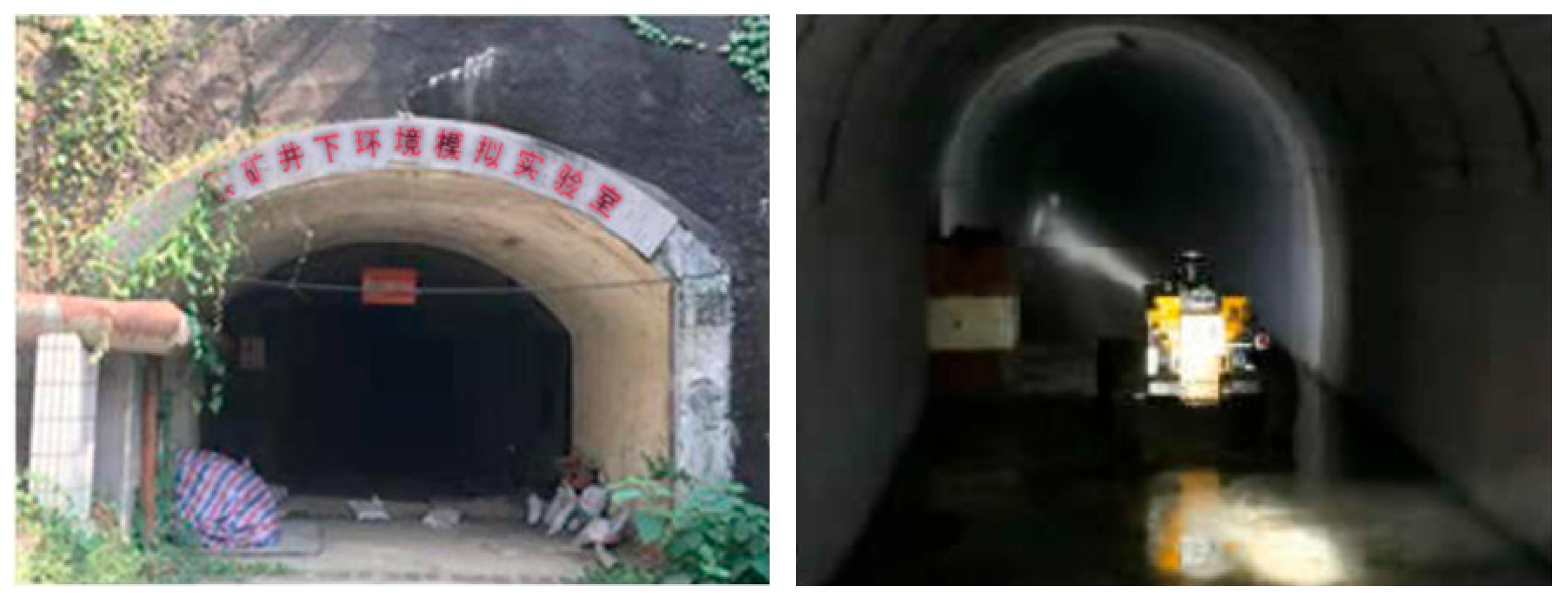
To make the proposed method more targeted, this study constructed the dataset based on the simulated roadway of China University of Mining and Technology, as shown in Figure 7. This simulated roadway is constructed in an equal proportion based on the arched roadway structure found in underground coal mines. It enables the simulation of typical environments such as the dim lighting conditions in underground coal mines.

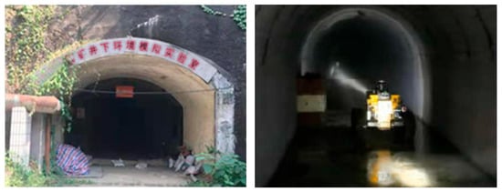
Figure 7. Simulated roadway in the coal mine underground environment simulation laboratory.

In this study, 300 infrared images collected from a simulated roadway were selected to construct an infrared dataset. To improve the stability of model training, data augmentation techniques were applied, expanding the dataset to 1200 images. For testing, 80% of the dataset was used as the training set, while 20% was reserved as the validation set.

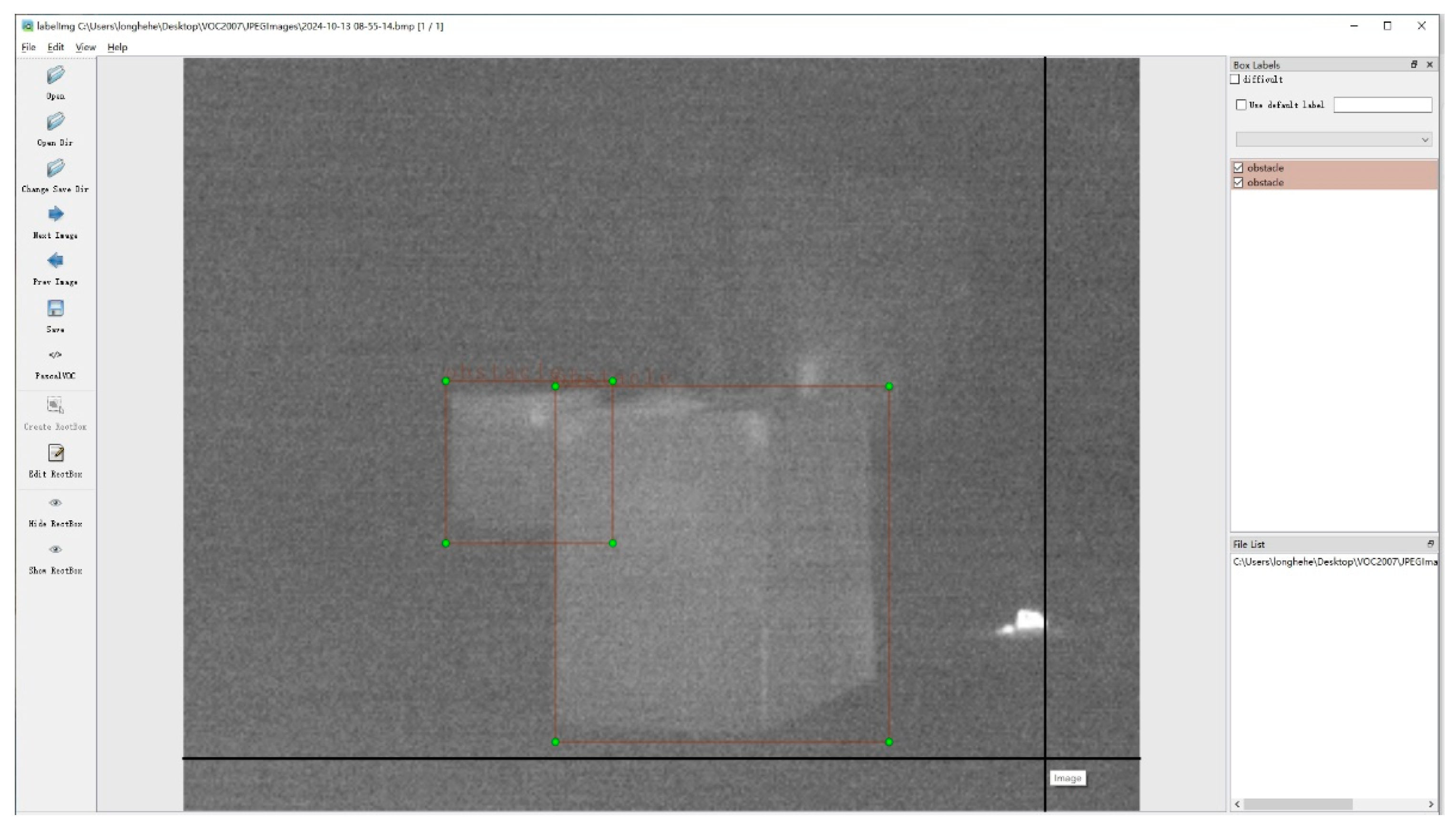
Before training the model, the dataset needed to be annotated. In this work, LabelImg v1.3.3 was used for image annotation. LabelImg is an open-source annotation tool that supports three formats: VOC (saved as XML files), YOLO (saved as TXT files), and CreateML (saved as JSON files). The VOC format was chosen for dataset annotation in this study. The annotation interface is shown in Figure 8.

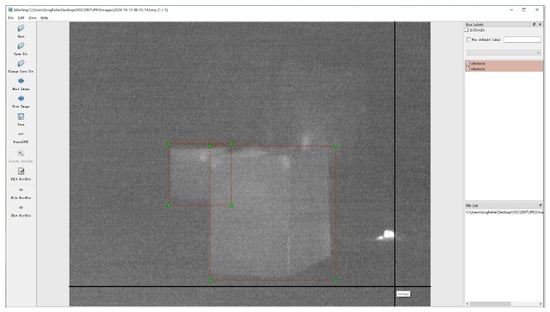
Figure 8. Labeling working interface.

4.2. Evaluation Metrics

In object detection tasks, evaluation metrics are the core basis for assessing model performance. Since object detection requires not only accurately locating the target but also correctly classifying its category, a single metric cannot comprehensively reflect the model’s capability. Proper evaluation metrics can quantify the model’s performance in terms of localization accuracy, classification correctness, and rates of missed or false detections.

• Intersection over Union (IoU): This metric measures the degree of overlap between the predicted bounding box and the ground truth bounding box and serves as a fundamental indicator in object detection tasks. Its formula is:

$$\mathrm{IOU}={\displaystyle \frac{A\cap B}{A\cup B}}$$

(14)

• Here, the numerator represents the area of the intersection between the predicted box and the ground truth box, while the denominator represents the area of their union. A higher IoU value indicates more accurate localization.
• Precision: The proportion of true positive samples among all samples predicted as positive by the model. Its formula is:

$$\mathrm{Precision}={\displaystyle \frac{TP}{TP+FP}}$$

(15)

• Recall: The proportion of true positive samples correctly predicted by the model among all actual positive samples. Its formula is:

$$\mathrm{Recall}={\displaystyle \frac{TP}{TP+FN}}$$

(16)

• In the above Formulas (12) and (13), the symbols $TP$, $FP$, and $FN$ represent True Positives, False Positives, and False Negatives, respectively.
• Average Precision (AP): A metric that combines Precision and Recall, evaluating the detection performance for a single class by calculating the area under the Precision-Recall curve (AUC). Its formula is:

$$AP={\displaystyle {\int }_0^{1}p\left(r\right)dr}$$

(17)

• Mean Average Precision (mAP): A comprehensive metric for multi-class detection tasks, calculated as the average of the AP values across all classes. Its formula is:

$$mAP={\displaystyle \frac{1}{N}}{\displaystyle \sum _{i=1}^{N}A{P}_i}$$

(18)

To evaluate the detection performance of the optimized YOLOv5 network, this study employs Precision, Recall, Average Precision (AP), and mean Average Precision (mAP), with mAP being the most critical metric due to its comprehensiveness.

4.3. Performance Comparison

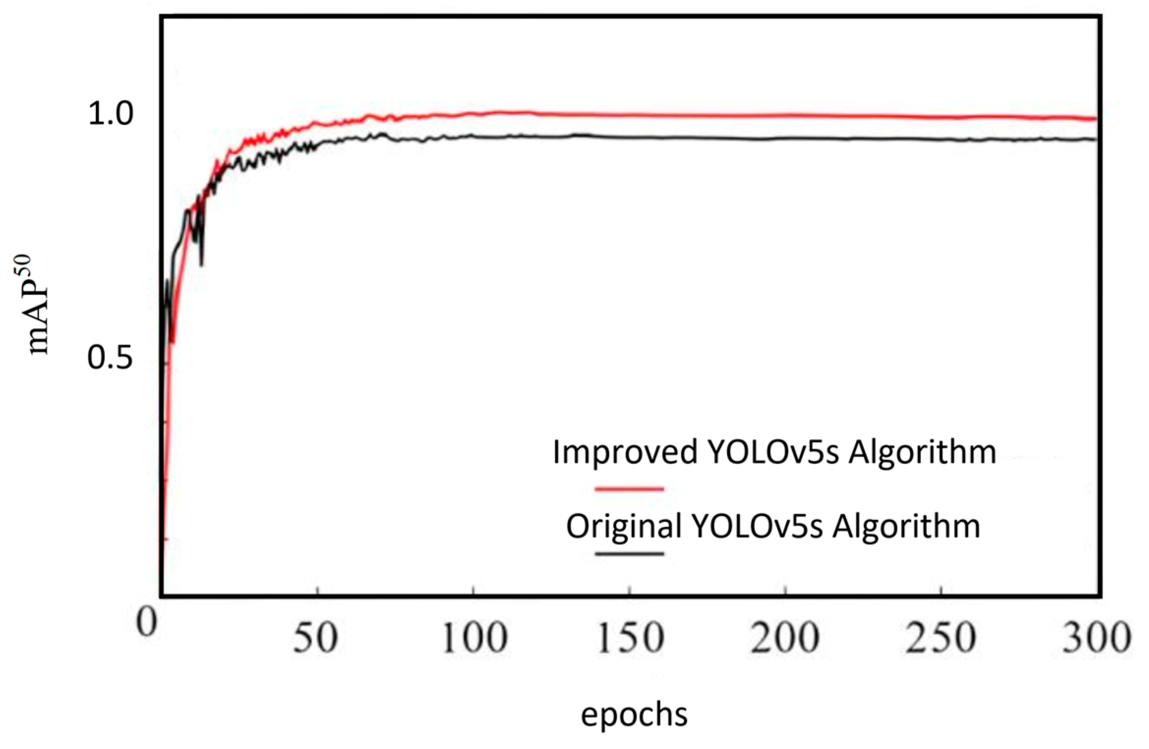
The optimization scheme proposed in this study not only makes the YOLOv5 model more lightweight and computationally efficient but also improves its accuracy to some extent, meeting the requirements for real-time data processing. Figure 9 shows a comparison of the original and improved models in terms of mAP50, providing a more intuitive view of the performance enhancement.

Figure 9. MAP50 comparison chart.

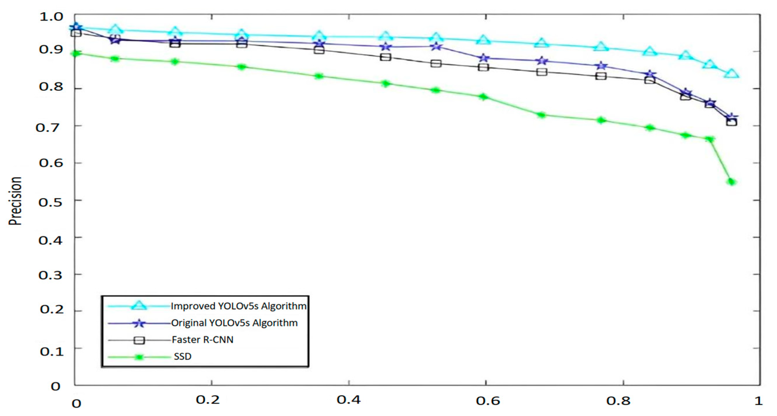
To validate the effectiveness of the YOLOv5 optimizations proposed in this study, the improved YOLOv5 was compared with SSD, Faster R-CNN, and the original YOLOv5. The experimental results are presented in Table 7.

Table 7. Performance comparison of various algorithms.

Algorithm	mAP/%	Detection Time (ms)	Parameters (MB)
SDD	73.2	52.6	25.0
Faster-RCNN	88.9	66.2	35.9
YOLOv5	91.5	45.3	7.2
Optimized YOLOv5	92.8	36.9	5.1

As shown in Table 7, the optimized YOLOv5 achieves the best performance in terms of mAP, detection time, and parameter size. Regarding detection accuracy, the optimized YOLOv5 improves mAP by 19.6% compared to SSD, by 3.9% compared to Faster-RCNN, and by 1.3% compared to the original YOLOv5. Due to its lightweight design, the optimized YOLOv5 has the smallest number of parameters, resulting in the shortest detection time and the fastest speed. The above indicators further demonstrate that the method proposed in this paper has superior detection reliability and detection speed, and possesses stronger comprehensive engineering application performance. The comparison of PR curves between the optimized YOLOv5 and other models is shown in Figure 10, from which it is evident that the optimized YOLOv5 significantly outperforms the other algorithms.

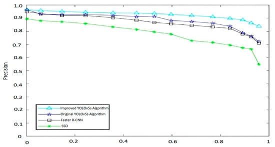
Figure 10. PR curve comparison chart.

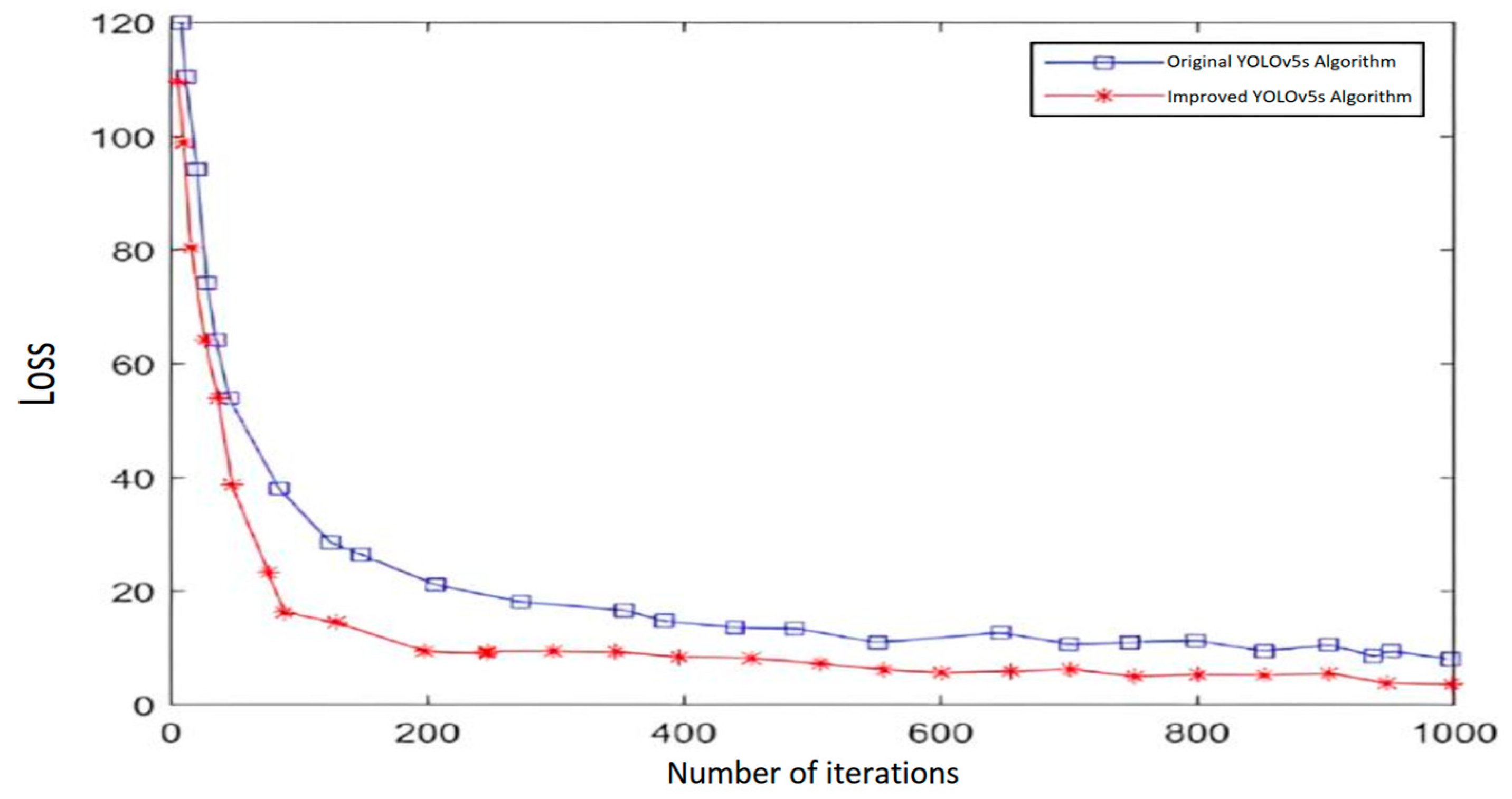
To evaluate the effectiveness of the network improvements, both the original YOLOv5 model and the optimized model were trained under the same conditions for comparison. Figure 11 shows the comparison of loss function changes for the two networks during training.

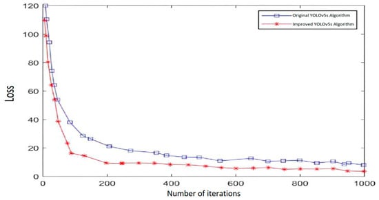
Figure 11. Loss function comparison diagram.

As shown in Figure 11, both models eventually achieve convergence. However, the optimized YOLOv5 model attains lower loss values and requires fewer iterations to stabilize. The original model stabilizes after approximately 350 iterations, whereas the improved YOLOv5 reaches stable convergence in about 200 iterations. These results indicate that the optimized YOLOv5 model demonstrates superior performance.

4.4. Millimeter-Wave Radar Information Supplement

Infrared cameras are less affected by the harsh underground roadway environment, providing stable performance in image data acquisition. Combined with the optimized YOLOv5, obstacles can be efficiently detected. However, infrared cameras cannot provide depth information and therefore cannot directly measure the actual distance to obstacles. Millimeter-wave (MMW) radar can compensate for this limitation by measuring the distance to objects through transmitting and receiving radio waves.

The 4D MMW radar can capture rich point cloud information when scanning the roadway environment. Obstacles or personnel in the mine, after being scanned by the radar, are represented by multiple sets of point clouds. Clustering algorithms can then be applied to separate point clouds corresponding to different obstacles.

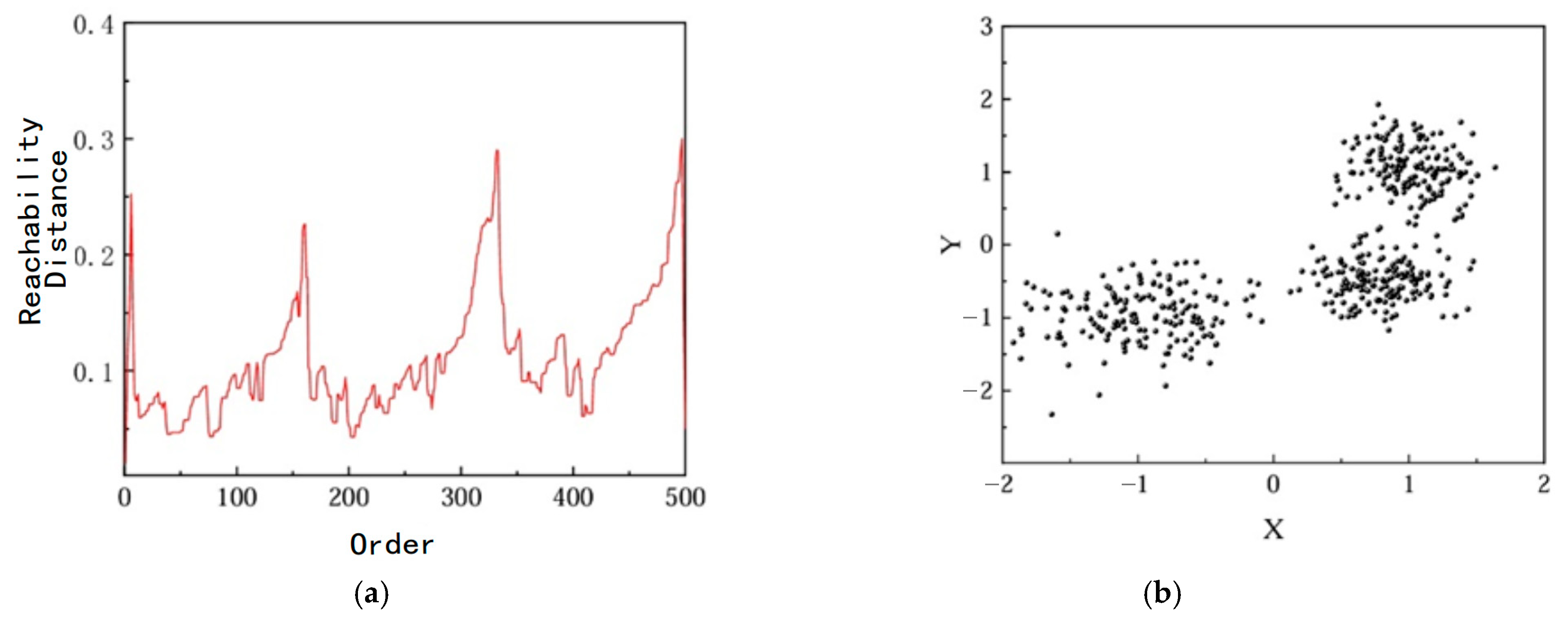
In this study, the Ordering Points To Identify the Clustering Structure (OPTICS [28]) algorithm is chosen for clustering the radar point cloud data. The core idea of OPTICS is to compute the core distance and reachability distance for each point, constructing an ordered sequence that reflects the clustering structure of the data. Unlike traditional clustering algorithms, OPTICS does not directly output clusters; instead, it generates a reachability plot from which clusters can be extracted based on different density thresholds. Applying OPTICS clustering to the radar point cloud data yields the results shown in Figure 12.

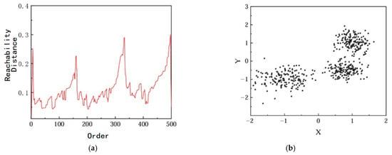
Figure 12. Results of the OPTICS clustering algorithm: (a) Reachability distance; (b) Original data.

From Figure 12, it can be seen that the optimized OPTICS clustering algorithm does not directly produce specific cluster labels. Instead, it sorts the data points based on their reachability distance, generating an ordered sequence. In Figure 12a, the vertical axis represents the reachability distance of each point. Shorter reachability distances indicate that points are more tightly packed. Valleys correspond to regions where several points have small reachability distances, meaning that points within the same valley have high local density and thus belong to the same cluster. Peaks indicate that a point has a large reachability distance to the previous point, suggesting that it belongs to a different cluster.

After clustering, a bounding box needs to be computed for each point cloud cluster. In this study, the Axis-Aligned Bounding Box (AABB) method is used to calculate the distance from the center of each clustered point cloud to the millimeter-wave radar origin. To increase point cloud density and improve visualization, a top-down view is adopted. This approach ignores the $\mathrm{Z}$-axis coordinate but allows the point cloud to appear denser in a 2D plane.

Since the $\mathrm{Z}$-axis values are no longer relevant, the 3D coordinates of the point cloud clusters are projected onto the $\mathrm{XY}$ plane. For each cluster’s $\mathrm{XY}$-plane point set, a 2D AABB is computed as follows:

$\mathrm{X}$-axis range: find the minimum and maximum $\mathrm{X}$ coordinates of all points, denoted as: $\mathrm{X}min=min(x1,x2,\dots )$ and $\mathrm{X}max=max(x1,x2,\dots )$.

$\mathrm{Y}$-axis range: find the minimum and maximum $\mathrm{Y}$ coordinates of all points, denoted as: $\mathrm{Y}min=min(y1,y2,\dots )$ and $\mathrm{Y}max=max(y1,y2,\dots )$.

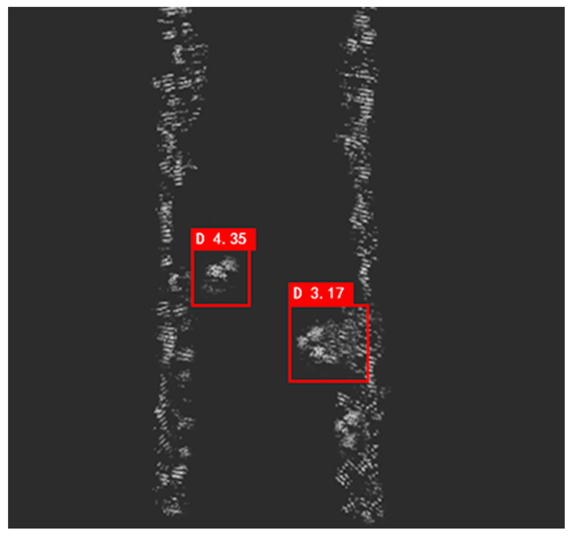
The center of the 2D AABB is calculated as: $c_x=(\mathrm{X}min+\mathrm{X}max)/2$ and $c_y=(\mathrm{Y}min+\mathrm{Y}max)/2$, denoted as $\left(c_x,\hspace{0.17em}{c}_y\right)$. The $\mathrm{Z}$-axis coordinate can be ignored. Let the millimeter-wave radar origin in the $\mathrm{XY}$ plane be $\left(0,\hspace{0.17em}0\right)$, and the cluster center be $\left(0,0\right)$. The Euclidean distance between these two points is: $\mathrm{distance}=\sqrt{c_x^2+c_y^2}$. Figure 13 illustrates the schematic of computing the point cloud cluster distance.

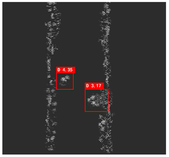
Figure 13. Schematic diagram of point cloud cluster distance.

From Figure 13, it can be seen that both the personnel and the obstacle are successfully detected. The distance from the personnel to the radar origin is 4.35 m, and the distance from the obstacle on the right to the origin is 3.17 m. Compared with the actual distances of 4.0 m and 3.0 m, the distance error for the personnel is 8.75%, and the error for the obstacle is 5.67%, both of which are less than 10%.

5. Experimental Study

To verify the feasibility and accuracy of the proposed underground roadway traversable area recognition system, a data acquisition and analysis platform based on an infrared camera and millimeter-wave radar was constructed. These sensors were reasonably arranged on a mobile robot to build an experimental platform for traversable area recognition. In this chapter, data are collected and processed in a simulated roadway to further validate the feasibility and accuracy of the improvements and optimization schemes proposed above.

5.1. Experimental Platform

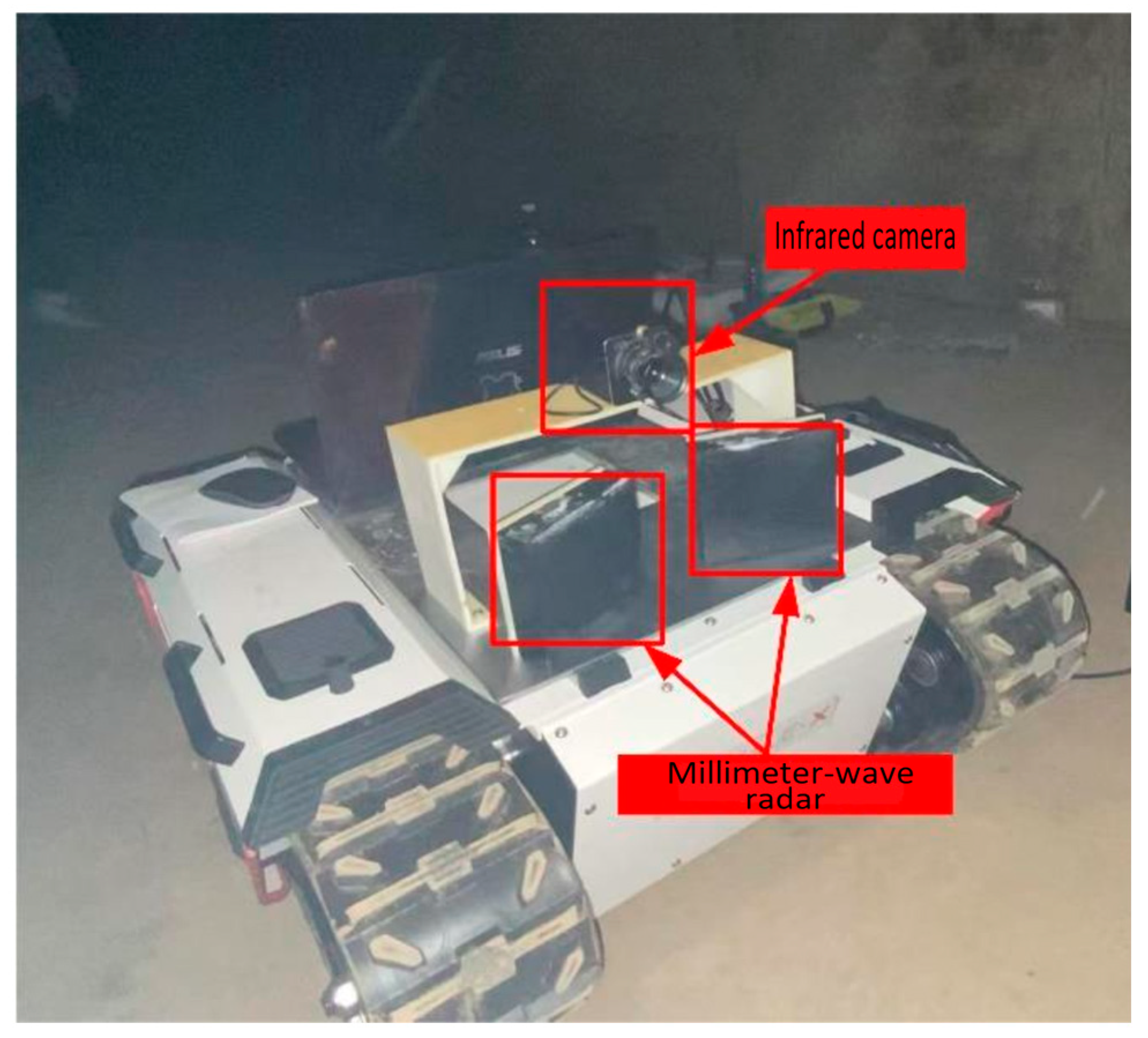
The experimental platform for the traversable area recognition system is built on a BUNKER tracked mobile robot which is produced by Songling Robot Co., Ltd. (Dongguan, China) and includes an infrared camera and two 4D millimeter-wave radars. In underground roadway environments, obstacles mainly consist of personnel and ground objects. The infrared camera captures general obstacle information, while the dual radars enhance perception accuracy, compensating for the limitations of the infrared camera and improving detection reliability. The sensors are mounted at the front of the robot, as shown in Figure 14, ensuring maximal coverage of the surrounding environment and stable operation in different roadway conditions. This configuration provides robust support for passable-area and obstacle recognition in complex underground settings.

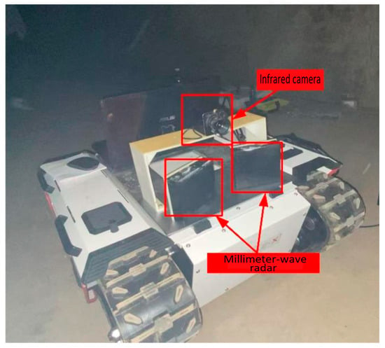
Figure 14. Schematic diagram of installation location for infrared camera and dual radar.

The height of the tracked robot is 400 mm; therefore, the central positions of the dual radars are 457.5 mm above the ground. The installation height of the infrared camera is 550 mm above the ground. Since the region of interest (ROI) of the millimeter-wave radars mainly focuses on the targets within the roadway boundaries, in order to obtain high-quality and dense point cloud data, the two radars are oriented at horizontal angles of +10° and –10° relative to the forward direction, with a center-to-center spacing of 200 mm. This installation configuration not only ensures that the sensors do not interfere with each other but also enables the acquisition of more accurate data, thereby achieving better detection performance.

5.2. Passable Area Recognition Experiment

To verify the practical application of the system, this section conducts a robot passable area recognition experiment in a simulated underground environment. The experimental scenario includes narrow tunnels, obstacles, and low-visibility conditions, aiming to replicate real coal mine underground working conditions.

For infrared target recognition, the YOLOv5 algorithm is used, primarily programmed in Python 3.8. The development kit provided by the infrared camera manufacturer is mainly in C++ and runs on Ubuntu 18.04. When using the infrared camera, the local IPv4 network and the camera’s IP must be set within the same subnet to ensure successful connection, after which data processing can proceed. Before activating the millimeter-wave radar, its spatial position must be configured through the parameters in the configuration file.

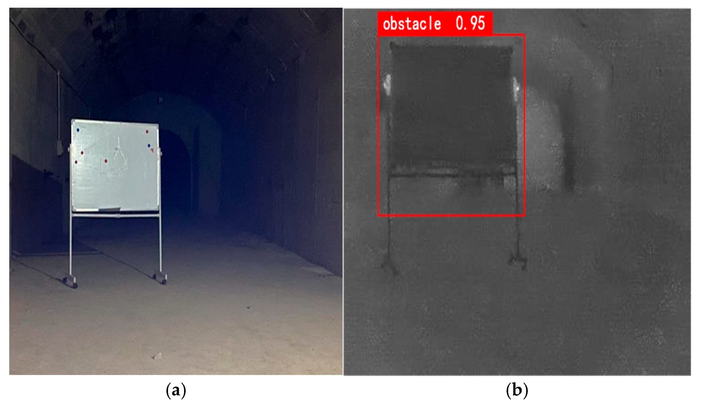
To meet the passable area recognition requirements for underground mobile robots, this study proposes a multimodal perception method based on an infrared camera and dual 4D millimeter-wave radars. The infrared camera provides target classification information, while the millimeter-wave radar supplements spatial depth data. By complementary fusion of these data sources, tunnel boundaries and obstacles can be accurately identified, enabling the delineation of passable areas. Using the infrared camera, the system captures infrared images of the obstacles and automatically determines their 2D positions and categories. Taking the board obstacle as an example, Figure 15 shows the recognition result.

Figure 15. Infrared Camera Recognition Results: (a) Actual position of the board; (b) Infrared image of the board.

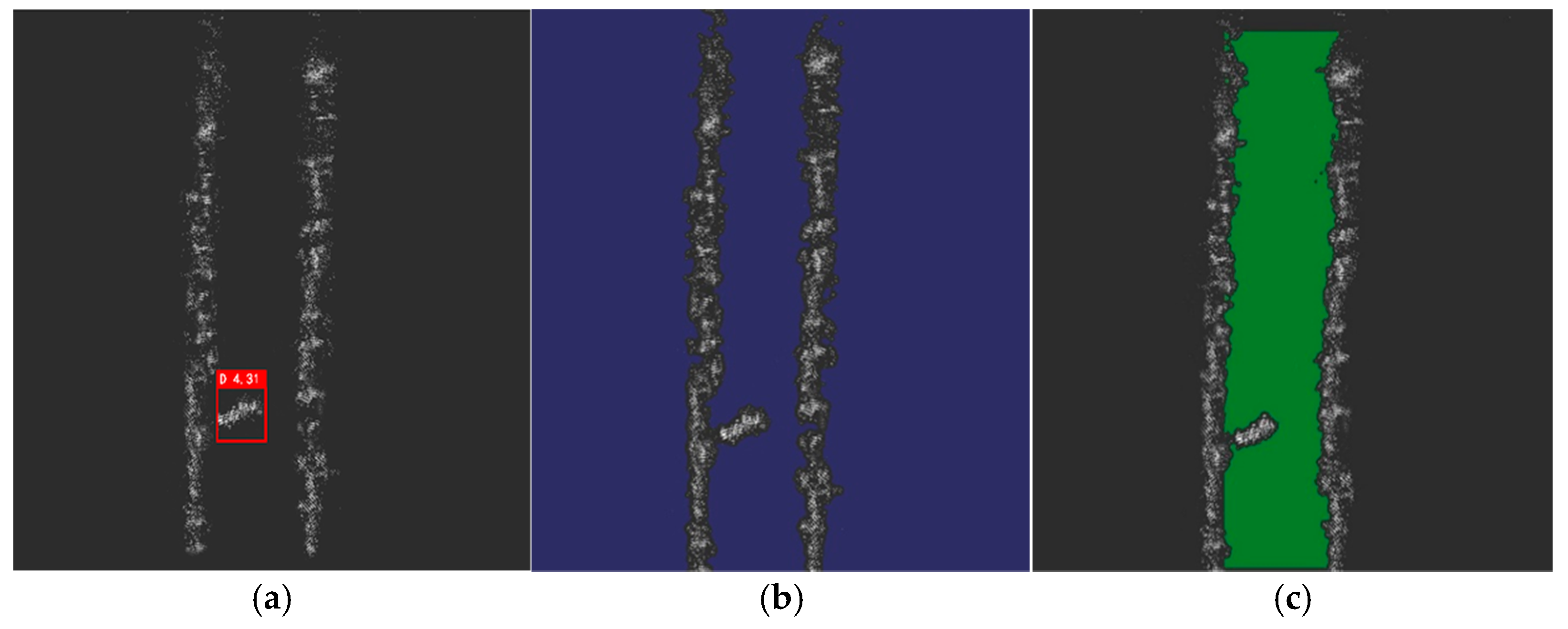
Through the processing of the aforementioned algorithm, the obstacle was successfully recognized with a confidence of 95%. Subsequently, the depth information of the obstacle was extracted from the millimeter-wave radar data and annotated with a detection box. To more clearly present the positions of the obstacle and the roadway boundaries, additional extraction processing was performed. In Figure 16, the non-blue regions indicate the locations of obstacles and roadway boundaries. Finally, the navigable area within the roadway was identified and marked, with the passable regions highlighted in green.

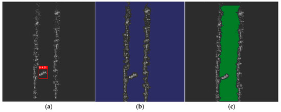
Figure 16. Millimeter-wave radar recognition results: (a) Distance information of the board; (b) Extraction results of obstacles and roadway boundaries; (c) Marked navigable area.

The above figures illustrate the precise location of the board obstacle in both the infrared images and the radar point cloud data. Using the navigable area marking algorithm, the obstacle and roadway boundaries are successfully labeled. The unmarked green area between the two roadway boundaries represents the navigable region. By combining the obstacle’s class and 2D position from the infrared images, the system effectively reduces the impact of obstacles on the robot’s movement within the roadway.

5.3. Experimental Effect Test

To verify the feasibility of the proposed system, experiments were conducted in an actual underground coal mine roadway. The test environment is shown in Figure 17, where the roadway contains pipelines, personnel, and ground obstacles.

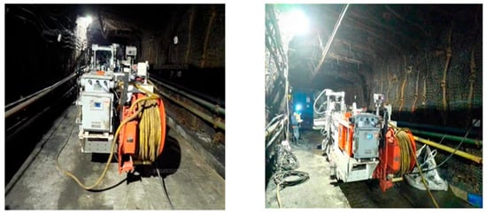
Figure 17. Underground experimental site.

A bottle-shaped obstacle was used to test the proposed algorithm and the UI display performance. The actual position of the obstacle in the roadway is shown in Figure 18. Using a distance meter, the actual Euclidean distance from the bottle obstacle to the origin of the millimeter-wave radar was measured as 4.0 m. The corresponding display result is shown in Figure 18.

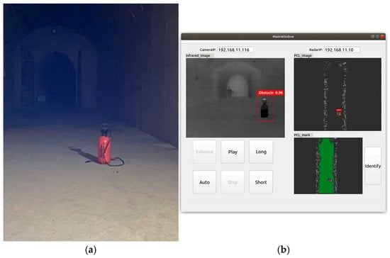
Figure 18. Bottle Obstacle Detection: (a) Actual Test Position of the Bottle Obstacle; (b) Display of Obstacle Detection Results.

From the UI display shown in Figure 18, it can be observed that the infrared camera feed and the millimeter-wave radar point cloud are successfully displayed simultaneously on the same interface, with the acquired data being processed in real time. The left display panel shows the infrared image, where the bottle obstacle is successfully recognized with a confidence score of 0.96. To present the target recognition results in a more intuitive way, the results of the indicator are as follows: the mAP is 90.1% and the detection time is 45.72. Although the performance of the core computing unit, namely AI computer, was affected due to its placement in the explosion-proof chamber, resulting in a slight decrease in the above results compared to the performance indicators in Table 7 during the industrial experiments, it still meets the identification requirements for personnel in underground coal mines.

Meanwhile, the right display panel shows the radar point cloud, where the obstacle’s point cloud cluster is detected, and the distance from the cluster center to the radar origin is measured as 4.28 m. Compared with the actual distance of 4.0 m measured by a rangefinder, the accuracy meets the requirements for obstacle detection in underground coal mines. It must be pointed out that the above distances are, respectively, quantified as the distances between the geometric center coordinates of the radar and the nearest point in the point cloud that represents the target to be detected (which is detected by the radar), and the approximate nearest position measured manually. In addition, the possible causes for the 0.28 m distance error (4.28 m vs. 4.00 m) mainly include the following aspects: (1) As millimeter-wave radar is a type of Doppler radar, its point cloud detection accuracy is relatively low; (2) The correspondence between the manually detected points and the automatically recognized points is inaccurate. After repeated tests, the average error of this system was 0.0923 m, and the maximum error was 0.3301 m. It still meets the actual application requirements in underground coal mines.

6. Conclusions

This study addresses the problem of traversable area recognition for autonomous mobile robots in the complex underground environment of coal mines, and proposes an environment perception method based on multimodal data fusion of infrared cameras and 4D millimeter-wave radar. By analyzing the harsh environmental characteristics of underground tunnels, such as low lighting, high dust concentration, and high humidity, a perception system composed of an infrared camera and dual 4D millimeter-wave radars was designed. Combined with an improved YOLOv5 object detection algorithm and optimized point cloud processing techniques, the system achieves high-precision obstacle recognition and dynamic delineation of traversable areas.

The research presented in this study is primarily based on infrared cameras and millimeter-wave radar, without exploring the fusion of other sensors such as visible-light cameras or LiDAR. Future work will involve incorporating additional sensor types and further investigating cross-optimization and compensation methods for multimodal sensors under different environmental scenarios. Meanwhile, due to the differences in the environmental scenarios of various coal mines, we have currently only tested the proposed method in simulated tunnels and some underground tunnel scenarios. In the future, we will expand the experimental scale to further optimize and improve the method presented in this paper, in order to enhance the adaptability of the algorithm and further promote its industrial application.

References

- Zhang, C.; Li, Z.; Li, J.; Zou, L.; Dong, E. Optimization of Visual Detection Algorithms for Elevator Landing Door Safety-Keeper Bolts. Machines 2025, 13, 790. [Google Scholar] [CrossRef]
- Sun, Z.; Tian, M.; Li, X. Control Strategy of PMSM for Variable Pitch Based on Improved Whale Optimization Algorithm. Machines 2025, 13, 872. [Google Scholar] [CrossRef]
- Kellner, D.; Klappstein, J.; Dietmayer, K. Grid-Based DBSCAN for Clustering Extended Objects in Radar Data. In Proceedings of the 2012 IEEE Intelligent Vehicles Symposium, Madrid, Spain, 3–7 June 2012; pp. 365–370. [Google Scholar] [CrossRef]
- Mousavian, A.; Anguelov, D.; Flynn, J.; Kosecka, J. 3D Bounding Box Estimation Using Deep Learning and Geometry. In Proceedings of the 2017 IEEE Conference on Computer Vision and Pattern Recognition (CVPR), Honolulu, HI, USA, 21–26 July 2017; pp. 7074–7082. [Google Scholar] [CrossRef]
- Prabhakara, A.; Jin, T.; Das, A.; Bhatt, G.; Kumari, L.; Soltanaghaei, E.; Bilmes, J.; Kumar, S.; Rowe, A. High Resolution Point Clouds from mmWave Radar. In Proceedings of the 2023 IEEE International Conference on Robotics and Automation (ICRA), London, UK, 29 May 2023; pp. 4135–4142. [Google Scholar] [CrossRef]
- Chen, X.; Kundu, K.; Zhu, Y.; Ma, H.; Fidler, S.; Urtasun, R. 3D Object Proposals Using Stereo Imagery for Accurate Object Class Detection. IEEE Trans. Pattern Anal. Mach. Intell. 2018, 40, 1259–1272. [Google Scholar] [CrossRef] [PubMed]
- Scheiner, N.; Appenrodt, N.; Dickmann, J.; Sick, B. Radar-Based Road User Classification and Novelty Detection with Recurrent Neural Network Ensembles. In Proceedings of the 2019 IEEE Intelligent Vehicles Symposium (IV), Paris, France, 9–12 June 2019; pp. 722–729. [Google Scholar] [CrossRef]
- Liu, B.; Zhang, Z.; Cai, H.; Zhang, R.; Wang, Z.; Yang, J. Self-Compensation Tensor Multiplication Unit for Adaptive Approximate Computing in Low-Power CNN Processing. Sci. China Inf. Sci. 2022, 65, 149403. [Google Scholar] [CrossRef]
- Liu, C.; Xie, F.; Zhang, H.; Jiang, Z.; Zheng, Y. Infrared Small Target Detection Based on Multi-Perception of Target Features. Infrared Phys. Technol. 2023, 135, 104927. [Google Scholar] [CrossRef]
- Nabati, R.; Qi, H. RRPN: Radar Region Proposal Network for Object Detection in Autonomous Vehicles. In Proceedings of the 2019 IEEE International Conference on Image Processing (ICIP), Taipei, Taiwan, 22–25 September 2019; pp. 3093–3097. [Google Scholar] [CrossRef]
- Nabati, R.; Qi, H. Radar-Camera Sensor Fusion for Joint Object Detection and Distance Estimation in Autonomous Vehicles. arXiv 2020. [Google Scholar] [CrossRef]
- Nobis, F.; Geisslinger, M.; Weber, M.; Betz, J.; Lienkamp, M. A Deep Learning-Based Radar and Camera Sensor Fusion Architecture for Object Detection. In Proceedings of the 2019 Sensor Data Fusion: Trends, Solutions, Applications (SDF), Bonn, Germany, 15–17 October 2019; pp. 1–7. [Google Scholar] [CrossRef]
- Sun, X.; Jiang, Y.; Qin, H.; Li, J.; Ji, Y. Camera-Radar Fusion with Radar Channel Extension and Dual-CBAM-FPN for Object Detection. Sensors 2024, 24, 5317. [Google Scholar] [CrossRef] [PubMed]
- Henriques, J.F.; Caseiro, R.; Martins, P.; Batista, J. Exploiting the Circulant Structure of Tracking-by-Detection with Kernels. In Proceedings of the Computer Vision—ECCV 2012; Fitzgibbon, A., Lazebnik, S., Perona, P., Sato, Y., Schmid, C., Eds.; Springer: Berlin/Heidelberg, Germany, 2012; pp. 702–715. [Google Scholar] [CrossRef]
- Liu, Y.; Zhang, Y.; Hu, M.; Si, P.; Xia, C. Fast Tracking via Spatio-Temporal Context Learning Based on Multi-Color Attributes and Pca. In Proceedings of the 2017 IEEE International Conference on Information and Automation (ICIA), Macao, China, 18–20 July 2017; pp. 398–403. [Google Scholar] [CrossRef]
- Danelljan, M.; Häger, G.; Khan, F.; Felsberg, M. Accurate Scale Estimation for Robust Visual Tracking. In Proceedings of the British Machine Vision Conference, Nottingham, UK, 1–5 September 2014; BMVA Press: London, UK, 2014. [Google Scholar] [CrossRef]
- Danelljan, M.; Häger, G.; Khan, F.S.; Felsberg, M. Discriminative Scale Space Tracking. IEEE Trans. Pattern Anal. Mach. Intell. 2017, 39, 1561–1575. [Google Scholar] [CrossRef] [PubMed]
- Li, Y.; Zhu, J. A Scale Adaptive Kernel Correlation Filter Tracker with Feature Integration. In Proceedings of the Computer Vision—ECCV 2014 Workshops; Agapito, L., Bronstein, M.M., Rother, C., Eds.; Springer International Publishing: Cham, Switzerland, 2015; pp. 254–265. [Google Scholar] [CrossRef]
- Bertinetto, L.; Valmadre, J.; Henriques, J.F.; Vedaldi, A.; Torr, P.H.S. Fully-Convolutional Siamese Networks for Object Tracking. In Proceedings of the Computer Vision—ECCV 2016 Workshops; Hua, G., Jégou, H., Eds.; Springer International Publishing: Cham, Switzerland, 2016; pp. 850–865. [Google Scholar] [CrossRef]
- Li, B.; Wu, W.; Wang, Q.; Zhang, F.; Xing, J.; Yan, J. SiamRPN++: Evolution of Siamese Visual Tracking with Very Deep Networks. In Proceedings of the 2019 IEEE/CVF Conference on Computer Vision and Pattern Recognition (CVPR), Long Beach, CA, USA, 15–20 June 2019; pp. 4282–4291. [Google Scholar] [CrossRef]
- Chen, X.; Yan, B.; Zhu, J.; Wang, D.; Yang, X.; Lu, H. Transformer Tracking. In Proceedings of the IEEE/CVF Conference on Computer Vision and Pattern Recognition, Online, 19 June–25 June 2021; pp. 8126–8135. [Google Scholar]
- Manduchi, R.; Castano, A.; Talukder, A.; Matthies, L. Obstacle Detection and Terrain Classification for Autonomous Off-Road Navigation. Auton. Robots 2005, 18, 81–102. [Google Scholar] [CrossRef]
- Krizhevsky, A.; Sutskever, I.; Hinton, G.E. ImageNet Classification with Deep Convolutional Neural Networks. Commun. ACM 2017, 60, 84–90. [Google Scholar] [CrossRef]
- Qi, C.R.; Su, H.; Mo, K.; Guibas, L.J. PointNet: Deep Learning on Point Sets for 3D Classification and Segmentation. In Proceedings of the 2017 IEEE Conference on Computer Vision and Pattern Recognition (CVPR), Honolulu, HI, USA, 21–26 July 2017; pp. 652–660. [Google Scholar] [CrossRef]
- Buades, A.; Coll, B.; Morel, J.-M. A Non-Local Algorithm for Image Denoising. In Proceedings of the 2005 IEEE Computer Society Conference on Computer Vision and Pattern Recognition (CVPR’05), San Diego, CA, USA, 20–25 June 2005; Volume 2, pp. 60–65. [Google Scholar] [CrossRef]
- Jocher, G.; Stoken, A.; Borovec, J. Ultralytics/Yolov5: V3.1—Bug Fixes and Performance Improvements. Zenodo 2020. [Google Scholar] [CrossRef]
- Ajayi, O.O.; Kurien, A.M.; Djouani, K.; Dieng, L. A Proactive Predictive Model for Machine Failure Forecasting. Machines 2025, 13, 663. [Google Scholar] [CrossRef]
- Kuwahara, A.; Kimura, T.; Okubo, S.; Yoshioka, R.; Endo, K.; Shimizu, H.; Shimada, T.; Suzuki, C.; Takemura, Y.; Hiraguri, T. Cluster-Based Flight Path Construction for Drone-Assisted Pear Pollination Using RGB-D Image Processing. Drones 2025, 9, 475. [Google Scholar] [CrossRef]
Disclaimer/Publisher’s Note: The statements, opinions and data contained in all publications are solely those of the individual author(s) and contributor(s) and not of MDPI and/or the editor(s). MDPI and/or the editor(s) disclaim responsibility for any injury to people or property resulting from any ideas, methods, instructions or products referred to in the content. |
© 2025 by the authors. Licensee MDPI, Basel, Switzerland. This article is an open access article distributed under the terms and conditions of the Creative Commons Attribution (CC BY) license (https://creativecommons.org/licenses/by/4.0/).