Abnormal Driving Area Detection Using Multiple Vehicle Dynamic Model-Based Filter: Design and Experimental Validation

Abstract

The main concern of remote control systems for autonomous ground vehicles (AGVs) is to perform the given mission according to the purpose of the operator. Although most remote systems are composed of a screen-based architecture, they are insufficient to transfer sufficient information to the remote operator. Therefore, in this paper, we present and experimentally validate an abnormal driving area detection system using an interacting multiple model (IMM) filter for the remote control system. In the proposed IMM filter, the unknown dynamic behavior of the vehicle, which changes according to changes in the driving environment, was lumped into a parameter change of the system model. As a result, we can obtain the probability of each model representing the reliability of each model, but an index can be used to infer the current status of the AGV and the driving environment. The index can help us detect both unusual behavior of the AGV such as skidding or sliding, and areas with low-friction road conditions that are not confirmed by images from the camera sensor. Thus, the remote operator can directly decide whether to continue operating or not. The proposed method is simple but useful and meaningful for the remote operator compared to the image-only method. The overall procedure of the proposed method was experimentally validated via a multi-purpose AGV on rough unpaved proving ground. Nine abnormal driving areas were discovered on the ground. In five of these areas, vehicles consistently exhibited abnormal driving behavior. The remaining four areas were confirmed to be affected by variables such as weather conditions and vehicle tire wear.

1. Introduction

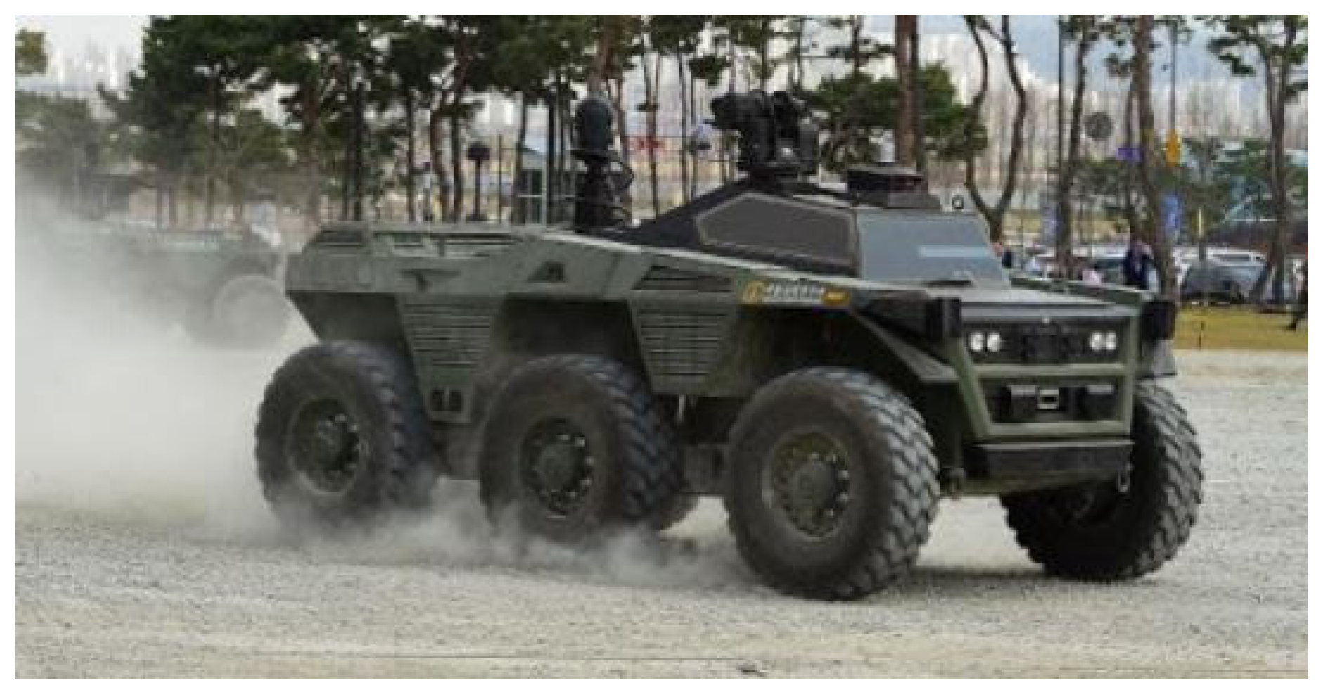
Autonomous ground vehicles (AGVs) have been studied to replace missions carried out by humans. In particular, they are widely used not only in industrial fields such as logistics and security robots but also in the defense field because they can handle tasks that are difficult or dangerous for humans to do. In the military field, AGVs are often used for missions such as detecting and removing landmines to minimize casualties. In addition, AGVs are also used for surveillance and reconnaissance of enemy forces [1,2,3,4]. To fulfill these special purposes and have solid durability, military AGVs are usually constructed in the form of skids, unlike ordinary passenger cars, as shown in Figure 1. The skid-type AGV steers with the speed difference between the left and right wheels and at the same time achieves the desired target speed. AGV includes both remote driving and autonomous driving types. In remote driving, the remote operator controls the AGV via a remote controller using communication over a long distance. The operator understands the driving situation through the AGV’s camera view displayed on the remote controller. Then, the operator judges the holistic situation and gives control commands to the vehicle to reach the desired destination. To enhance the operator’s driving realism, the operator often controls the AGV through the screen of the control system decorated as if in a vehicle such as a virtual reality headset or 360-degree screen [5,6]. Nevertheless, when the driving environment is transmitted only through the screen, there is a problem that it is difficult for the operator to feel a sense of reality because vibration and sound felt in the actual driving environment are not transmitted. In particular, it is difficult to distinguish whether a skid-type vehicle is skidding due to steering or slipping due to the driving environment because a skid-type vehicle steers with a difference in speed between the left and right wheels.

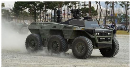
Figure 1. Target test autonomous ground vehicle.

AGVs in the form of autonomous driving are widely used in enemy surveillance and reconnaissance missions. When the operator remotely selects the mission area, the AGV itself performs all perception, decision, and control. A global path for a given environment and map is automatically planned considering topographic information. Both perception and decision are continuously repeated during trips through sensors such as cameras and lidars. Consequently, a local path is calculated in a path-planning algorithm that can simultaneously achieve both objectives, avoiding dynamic obstacles and following the global path [7]. Then, the controller autonomously controls the AGV to follow the planned local path. The operator checks in real time whether autonomous driving is working well from a remote location and, if necessary, immediately converts to remote control mode for control. Many researchers have studied stable and reliable autonomous driving in various fields such as object classification using convolutional neural networks [8,9], planning an optimal path to avoid dynamic obstacles [10,11], understanding driving scenes using artificial intelligence, and model predictive control techniques considering vehicle constraints [12]. Combined envelope control techniques for AGVs, including both active front steering and direct yaw-moment control, are proposed in [13]. To guarantee robustness against unknown disturbance, a backstepping control approach for path control with an extended-state observer was also proposed [14]. In [15], the polytopic method was introduced to characterize the time-varying vehicle speed while using fewer vertices to simplify the control scheme. However, such autonomous driving research has mainly been performed in well-known environments such as highways and racing tracks. One of the problems that must be overcome for AGVs is exploring and driving autonomously on uncertain rough terrain that has not been visited. In particular, AGVs do not run on roads paved with asphalt but mainly drive on unpaved roads or rough terrain.

2. Related Work

In this paper, a practical AGV monitoring system using interacting multiple models (IMMs) is presented to overcome the problem that it is difficult for the operator to feel the reality of remote driving and the stability problem caused by the uncertain road environment during autonomous driving. The IMM filter has been developed as a cost-effective suboptimal hybrid state estimation scheme [16]. It also has the advantages of requiring low computational power and giving high performance. The IMM method has mainly been developed in aerospace studies for the accurate tracking and estimation of multiple targets [17,18,19]. Recently, researchers have also used IMM to evaluate the reliability of each model. In autonomous vehicle applications, analysis of the vehicle motion between kinematics and dynamics [20,21] was proposed. Fault detection based on the probability of each model [22,23] was also introduced. Considering the reliability characteristic of each model, we design an abnormal driving area detection system which can detect and monitor unintended vehicle motion, especially slippage. The procedure of the proposed system for skid-type AGVs is as follows. The possible vehicle driving situations are represented by several dynamic motion models with various cornering stiffness levels. We have determined these cornering stiffness values through numerous experiments under various experimental conditions in advance. And the IMM filter calculates and updates the probability of each model in real time. These probabilities are used as an indicator of the abnormal driving area detection system to determine which models are more reliable. As a result, the remote operator can clearly understand the driving situation of the AGV. By observing the indicators of the monitoring system, the operator can decide whether it will continue to operate or not. Furthermore, the overall procedure of the proposed method was experimentally validated via a multi-purpose AGV and verified through numerous field experiments. The main contributions of the proposed method can be summarized as follows:

• The dynamic behavior of the vehicle, which changes according to the change of the driving environment, is expressed as a parameter change of the system model.
• It is possible to indirectly check the status of the vehicle even on the unvisited and unknown area from the probability value obtained through the interaction of multiple models.
• The proposed method is the first approach for 6x6 skid-type AGV and the overall procedure of the proposed method was experimentally validated via a multi-purpose AGV on the rough proving ground test.

In remote driving, the proposed scheme is helpful to check the degree of slippage of the vehicle. By indicating whether the vehicle is in a stable driving state or not, the proposed method can overcome the problem that the operator cannot feel the reality of remote driving. In addition, in autonomous driving, it is possible to determine the road surface condition of the driving area based on the reconnaissance information. The proposed method has the advantage of designing multiple models for specific parameters and obtaining reliability based on probability values, unlike the state-of-the-art designing and classifying various models of vehicle movement. Furthermore, the proposed method can determine whether the stability of autonomous driving control in the reconnaissance area is well maintained, so it is helpful to formulate a control strategy for subsequent reconnaissance vehicles.

3. Vehicle Model

To design a model-based vehicle abnormal driving area detection system, a simple lateral dynamic motion model of a skid-type vehicle is presented in this section. And, a vehicle status indexing scheme is also covered by specifying certain tire cornering stiffness.

3.1. Lateral Vehicle Dynamics

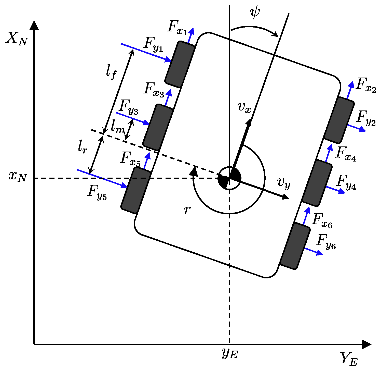
The dynamic motion model of the 6 × 6 skid-type ground vehicle is briefly described in this section. The structure and coordinate frames are shown in Figure 2. The equation lateral motion for the given 6 × 6 skid-type vehicle is obtained as follows

$$\begin{array}{c}\hfill m(\ddot{y}+r{v}_x)=F_{yf}+F_{ym}+F_{yr}.\end{array}$$

(1)

m, $\ddot{y}$, r, and $v_x$ denote mass, lateral acceleration, yaw rate, and longitudinal velocity of the vehicle, respectively. The lateral tire force, $F_y$, can be written with the cornering stiffness of the tire and tire slip angle as follows:

$$\begin{array}{cc}\hfill F_{yf}& =F_{y1}+F_{y2}=2C_{{\alpha }_f}{\alpha }_f,\hfill \\ \hfill F_{ym}& =F_{y3}+F_{y4}=2C_{{\alpha }_m}{\alpha }_m,\hfill \\ \hfill F_{yr}& =F_{y5}+F_{y6}=2C_{{\alpha }_r}{\alpha }_r,\hfill \end{array}$$

(2)

where the slip angle of the tire, $\alpha$, is defined as the negative value of the velocity vector’s orientation due to the orientation of the tire is always zero for the skid-type vehicle.

$$\begin{array}{c}\hfill \alpha =-{\theta }_v,\end{array}$$

(3)

where ${\theta }_v$ is the angle that the velocity vector makes with the longitudinal axis of the vehicle. Now, one can make use of the following relations to calculate ${\theta }_{v_f}, {\theta }_{v_m}$ and ${\theta }_{v_r}$ considering the relative position between each wheel and the center of gravity, respectively.

$$\begin{array}{cc}\hfill tan({\theta }_{v_f})& ={\displaystyle \frac{v_y+l_{f}r}{v_x}},\hfill \\ \hfill tan({\theta }_{v_m})& ={\displaystyle \frac{v_y+l_{m}r}{v_x}},\hfill \\ \hfill tan({\theta }_{v_r})& ={\displaystyle \frac{v_y-l_{r}r}{v_x}}.\hfill \end{array}$$

(4)

$l_f$, $l_m$, and $l_r$ denote the distance from the center of gravity to each wheel, respectively. Substituting from (2)–(4) into (1) using small-angle approximation and $\dot{y}=v_y$, the lateral motion equation can be written as

$$\begin{array}{c}\hfill \ddot{y}=-{\displaystyle \frac{2(C_{\alpha f}+C_{\alpha m}+C_{\alpha r})}{m{v}_x}}\dot{y}-v_{x}r+{\displaystyle \frac{2(C_{\alpha f}{l}_f+C_{\alpha m}{l}_m-C_{\alpha r}{l}_r)}{m{v}_x}}r,\end{array}$$

(5)

where $C_f$ denotes the cornering stiffness of the tire. One can make use of the following equation for the yaw dynamics:

$$I_z\dot{r}=M_z,$$

(6)

where $I_z$ and $M_z$ denote the moment of inertia and lateral moment, respectively. Let us define the state $\mathbf{x}={\left[\dot{y}r\right]}^T$ and the input $u=M_z$. Then, the state space representation of the overall vehicle motion can be written as

$$\begin{array}{cc}\hfill \dot{\mathbf{x}}& =A\mathbf{x}+Bu\hfill \end{array}$$

(7)

where

$$\begin{array}{c}\hfill A=\left[\begin{array}{cc}{a}_{11}& a_{12}\\ 0& 0\end{array}\right],B=\left[\begin{array}{c}0\\ b_{21}\end{array}\right],\end{array}$$

with

$$a_{11}=-{\displaystyle \frac{2(C_{\alpha f}+C_{\alpha m}+C_{\alpha r})}{m{V}_x}},$$

$$a_{12}=-V_x-{\displaystyle \frac{2(C_{\alpha f}{l}_f+C_{\alpha m}{l}_m-C_{\alpha r}{l}_r)}{m{V}_x}},b_{21}={\displaystyle \frac{1}{I_z}}.$$

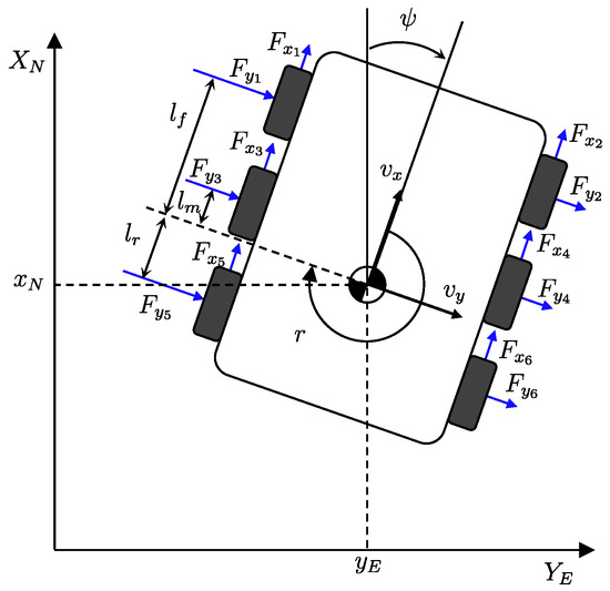
Figure 2. Base structure and coordinate frames.

3.2. Cornering Stiffness

The tire cornering stiffness is the coefficient representing the relationship between the tire slip angle and the lateral tire force. However, it is quite difficult to determine the value of cornering stiffness because of its nonlinearity [24]. This cornering stiffness varies according to the external environment conditions such as vertical tire force, and road friction. In particular, the stiffness also changes as the tire slip angle changes, as shown in Figure 3. It can be seen that the higher the tire–road friction (asphalt) and the smaller the tire slip angle, the larger the coefficient value. Therefore, once the coefficient values are specified, one can indirectly infer the tire slip angle and know the situation in which the vehicle is slipping. So, we design a multiple model for various cornering stiffnesses depending on the driving environment and specify the stiffness to index the vehicle status.

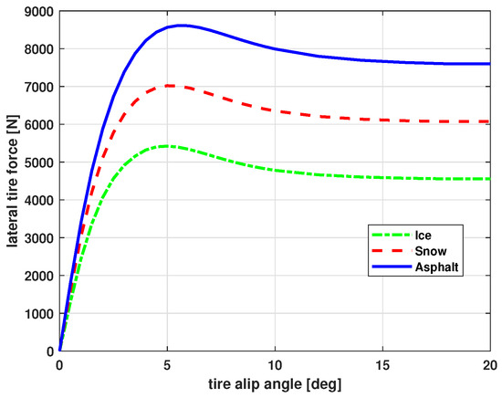
Figure 3. Example of cornering stiffness characteristics.

In this paper, we obtained the nominal cornering stiffness of the tire via simulation from the TruckSim simulator released from the mechanical simulation. The vehicle and tire models were set as close to the real one as possible, and the cornering stiffness of the tire was calculated through simulation results. In the next section, we are about to develop multiple models to specify the unmeasurable and nonlinear varying cornering stiffness. Consequently, an interacting multiple model (IMM) filter-based abnormal driving area detection system is presented.

4. Interacting Multiple Model

An interacting multiple model (IMM) filter has been developed as the cost-effective suboptimal hybrid state estimation scheme [17,18]. In this paper, we use the IMM filter to specify the cornering stiffness and infer the status of the vehicle for remote control. The cornering stiffness according to the slip of the vehicle is defined in advance, and the status of the vehicle is determined by monitoring the state and probability from the IMM filter. The overall proposed structure is described in Figure 4. The IMM filter consists of four steps: interaction, filtering, updating, and combination.

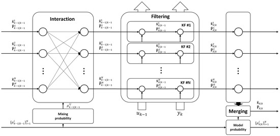
Figure 4. Block diagram of the IMM filter for N-models.

The IMM begins with the selection of a set of candidate models, each representing a different hypothesis about the system dynamics. These models can vary in complexity and may capture different aspects of the system behavior. The IMM incorporates mode transition probabilities, which govern the likelihood of the system switching from one model to another over time. These probabilities are typically estimated based on the system’s history or predefined rules. Mode transition probabilities play a crucial role in adapting the IMM framework to changes in the system dynamics. The core of IMM involves the filtering or estimation process, where the outputs of multiple models are combined to generate an optimal estimate of the system state. Each model’s output is weighted according to its current mode probability, reflecting the confidence in that model’s prediction. After the filtering step, the mode probabilities and model weights are updated based on the observed data. This update process ensures that models that provide more accurate predictions are given higher weights in subsequent iterations, while less accurate models are down-weighted. Weight update strategies can vary depending on the specific IMM implementation and application requirements. Once the filtering process is complete, the estimated system state can be used for prediction or control purposes. In prediction tasks, IMM can provide more accurate forecasts by leveraging the diversity of multiple models.

4.1. Multiple Model Setting

Let us consider the state space model using model index $n\in \{1,\dots ,N\}$ according to the cornering stiffness.

$$\begin{array}{cc}\hfill x_{k+1}& ={\Phi }^{\left(n\right)}{x}_k+{\Gamma }^{\left(n\right)}{u}_k+w_k^{\left(n\right)}\hfill \\ \hfill y_k& =C^{\left(n\right)}{x}_k+v_k^{\left(n\right)}\hfill \end{array}$$

(8)

where $w_k^{\left(n\right)}\sim N(0,Q^{\left(n\right)})$ and $v_k^{\left(n\right)}\sim N(0,R^{\left(n\right)})$. Here, we assume that the model index at time k, $n_k$, is modeled as a time-invariant Markov chain with transition probability matrix $\Pi$ as follows:

$$\Pi =\{{\pi }_{ij}=P(n_{k+1}=i|n_k=j)\},$$

(9)

where $i,j\in \{1,\dots ,N\}$ and ${\pi }_{ij}$ denotes the Markov probability of a transition from model j to i.

4.2. Interaction of Multiple Model

Let us define the probability of model i at time k as ${\mu }_{k|k}^i$. The model probability represents the likelihood that a particular mode best describes the system state at a given time. This probability is calculated based on the degree of match between the mode’s state estimate and the actual observations. Then, we can represent the mixing probability ${\mu }_{k-1|k-1}^{ij}$ using the model probability as follows:

$$\begin{array}{c}\hfill {\mu }_{k-1|k-1}^{ij}={\displaystyle \frac{{\pi }_{ij}{\mu }_{k-1|k-1}^j}{{\overline{c}}_i}},\end{array}$$

(10)

where the normalization factor is

$$\begin{array}{cc}\hfill {\overline{c}}_i& =\sum _{j=1}^N{\pi }_{ij}{\mu }_{k-1|k-1}^{ij}.\hfill \end{array}$$

(11)

Here, the mixing probability indicates the likelihood of transitioning between different modes, providing information on how modes might change over time. It is computed by combining the previous time’s mode probabilities with the current time’s mode transition probabilities.

Then, the mixed initial state ${\tilde{\mathbf{x}}}_{k-1|k-1}^i$ and the mixed initial covariance ${\tilde{\mathbf{P}}}_{k-1|k-1}^i$ of model i at sample time $k-1$ are given by

$$\begin{array}{cc}\hfill {\tilde{\mathbf{x}}}_{k-1|k-1}^i=& \sum _{j=1}^N{\mu }_{k-1|k-1}^{ij}{\widehat{\mathbf{x}}}_{k-1|k-1}^j\hfill \\ \hfill {\tilde{\mathbf{P}}}_{k-1|k-1}^i=& \sum _{j=1}^N{\mu }_{k-1|k-1}^{ij}\left[{\widehat{\mathbf{P}}}_{k-1|k-1}^j+({\widehat{\mathbf{x}}}_{k-1|k-1}^j-{\tilde{\mathbf{x}}}_{k-1|k-1}^i)\right.\left.{({\widehat{\mathbf{x}}}_{k-1|k-1}^j-{\tilde{\mathbf{x}}}_{k-1|k-1}^i)}^T\right],\hfill \end{array}$$

(12)

where ${\widehat{\mathbf{x}}}_{k-1|k-1}^j$ and ${\widehat{\mathbf{P}}}_{k-1|k-1}^j$ denote the estimated state and covariance of model j at sample time $k-1$, respectively. Then, each single Kalman filter using model indexed i starts filtering with this mixed initial state and covariance.

4.3. Filtering

Remark 1.

For the given 6 × 6 skid-type lateral motion model, only the system matrix Φ is changed by the cornering stiffness. Therefore, the input matrix Γ and the measurement matrix C for each model are exactly the same as each other. Thus, the following measurement matrix C is used in each model.

$$\begin{array}{c}\hfill C=\left[\begin{array}{cc}1& 0\\ 0& 1\end{array}\right].\end{array}$$

(13)

Now, the prediction and correction of both state and covariance are performed by each single Kalman filter.

4.3.1. Prediction

The prediction of both state and covariance is calculated using the system model in (1) and mixed initial values.

$$\begin{array}{cc}\hfill {\overline{\mathbf{x}}}_{k|k-1}^i& ={\Phi }_{k-1}^i{\tilde{\mathbf{x}}}_{k-1|k-1}^i+\Gamma {\mathbf{u}}_{k-1}\hfill \\ \hfill {\overline{\mathbf{P}}}_{k|k-1}^i& ={\Phi }_{k-1}^i{\tilde{\mathbf{P}}}_{k-1|k-1}^i{\left({\Phi }_{k-1}^i\right)}^T+Q_{k-1}^i,\hfill \end{array}$$

(14)

where ${\overline{\mathbf{x}}}_{k|k-1}^i$ and ${\overline{\mathbf{P}}}_{k|k-1}^i$ denote the predicted value at time k calculated from sample time $k-1$ for model i. ${\Phi }_{k-1}^i$ denotes the system matrix for model i with the cornering stiffness $C_{\alpha f}^i$, $C_{\alpha m}^i$, $C_{\alpha r}^i$ at time $k-1$. For simplification, we set $C_{\alpha f}^i=C_{\alpha m}^i=C_{\alpha r}^i$.

4.3.2. Correction

The correction of state and covariance is calculated using both the measurement and the predicted values.

$$\begin{array}{cc}\hfill S_k^i& =C{\overline{\mathbf{P}}}_{k|k-1}^i{C}^T+R_{k-1}^i\hfill \\ \hfill {\mathbf{K}}_k^i& ={\overline{\mathbf{P}}}_{k|k-1}^i{C}^T{\left(S_k^i\right)}^{-1}\hfill \\ \hfill {\widehat{\mathbf{x}}}_{k|k}^i& ={\overline{\mathbf{x}}}_{k|k-1}^i+{\mathbf{K}}_k^i({\mathbf{y}}_k^i-C{\overline{\mathbf{x}}}_{k|k-1}^i)\hfill \\ \hfill {\widehat{\mathbf{P}}}_{k|k}^i& =(I-{\mathbf{K}}_k^{i}C){\overline{\mathbf{P}}}_{k|k-1}^i\hfill \end{array}$$

(15)

where ${\mathbf{y}}_k^i$ and $S_k^i$ are innovation and its covariance filter using model i, respectively.

Remark 2.

For the given system, the measurement $y_k^i$ is exactly the same as each other for all i.

The correction of both state and covariance is used when calculating the initial value of the mixing step in the next iteration.

4.4. Updating

The likelihood function of each model i at time k, ${\Lambda }_k^i$, is given by the Gaussian assumption

$$\begin{array}{c}\hfill {\Lambda }_k^i={\displaystyle \frac{\exp [-\left(\frac{1}{2}\right){\left({\mathbf{y}}_k^i\right)}^T{\left(S_k^i\right)}^{-1}\left({\mathbf{y}}_k^i\right)]}{|2\pi S_k^i{|}^{\frac{1}{2}}}}.\end{array}$$

(16)

Then, the model probabilities of each model are calculated as follows:

$$\begin{array}{cc}\hfill {\mu }_{k|k}^i& ={\displaystyle \frac{1}{c}}{\Lambda }_k^i\sum _{j=1}^N{\pi }_{ij}{\mu }_{k-1|k-1}^j\hfill \\ & ={\displaystyle \frac{1}{c}}{\Lambda }_k^i{\overline{c}}_i,\hfill \end{array}$$

(17)

where c is the normalization factor for ${\sum }_{i=1}^N{\mu }_{k|k}^i=1$.

4.5. Merging

The merged state ${\widehat{\mathbf{x}}}_{k|k}$ and its covariance ${\widehat{\mathbf{P}}}_{k|k}$ are calculated as follows using the standard Gaussian mixture mean and covariance formula

$$\begin{array}{cc}\hfill {\widehat{\mathbf{x}}}_{k|k}& =\sum _{i=1}^N{\mu }_{k|k}^i{\widehat{\mathbf{x}}}_{k|k}^i\hfill \\ \hfill {\widehat{\mathbf{P}}}_{k|k}& =\sum _{i=1}^N{\mu }_{k|k}^i[{\widehat{\mathbf{P}}}_{k|k}^i+({\widehat{\mathbf{x}}}_{k|k}^i-{\widehat{\mathbf{x}}}_{k|k}){({\widehat{\mathbf{x}}}_{k|k}^i-{\widehat{\mathbf{x}}}_{k|k})}^T].\hfill \end{array}$$

(18)

Note that the correction of both state and covariance of each filter is used recursively to compute the initial mixed value of each filter in the next step, but the fused state and covariance are not. The convergence of the IMM filter with theoretical proof is detailed in [25].

4.6. Indexing

We can make use of the model probabilities at every sample time in Equation (17). Therefore, this model probability, ${\mu }_{k|k}^i$, is adopted for the abnormal driving area detection system. We set four models $(N=4)$ considering AGV driving conditions using cornering stiffness. The highest probability from the IMM filter indicates the current status of AGV (1: Danger; 2: Semi-Danger; 3: Semi-Stable; 4: Stable). For example, the lowest cornering stiffness represents the Danger ($n=1$). The low stiffness indicates a situation where the ground is frozen or the tire slip angle is large. Then, we can infer that the vehicle is in a state of severe slippage. On the other hand, a high stiffness means that the tire–road friction coefficient is high or the tire slip angle is small ($n=4$). Consequently, it can be inferred that the vehicle is driving stably.

5. Experiment Results

5.1. Experiment Setup

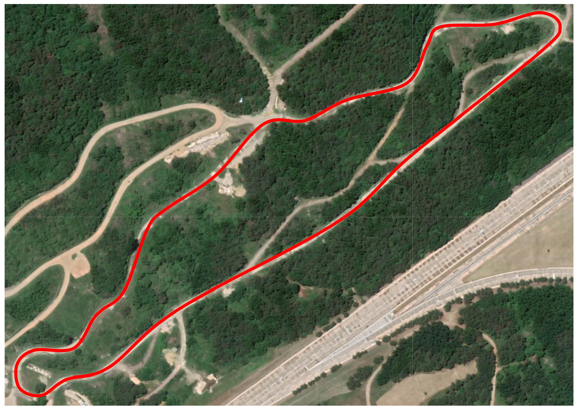
The proposed monitoring system was validated through several field tests on the unpaved proving ground as shown in Figure 5. For the field tests, the 6 × 6 skid-type AGV shown in Figure 1 is used. The AGV weighing more than 5000 [kg] is powered by a hybrid engine consisting of a gasoline engine and battery connected in series. And its maximum speed is about 40–50 [kph]. Various sensors such as inertial measurement unit (IMU), global positioning system (GPS), 2/3D LiDAR, and cameras were implemented on the AGV to perceive the uncertain and unknown driving environment and to measure the state of the dynamic model. The algorithm of AGV is composed of perception, planning, and control components. A remote operating control system is also utilized to interact with the AGV. Control commands such as speed, stop/start, and reconnaissance points are transmitted to the AGV, and vehicle state information such as images from the camera and current global position is received from the remote control system. The global and local path planning proceeded sequentially in the path planning algorithm using the reconnaissance points [26]. During the path planning and control, the multi-sensor fusion algorithm using 3D range registration was utilized in the experiments to enhance the robustness and accuracy of AGV localization against vulnerable GPS data from external disturbances [27]. The robust path controller using a disturbance observer was implemented for the path control. The proposed method is not integrated into the controller. The overall IMM procedure was processed through post-processing after the completion of each driving.

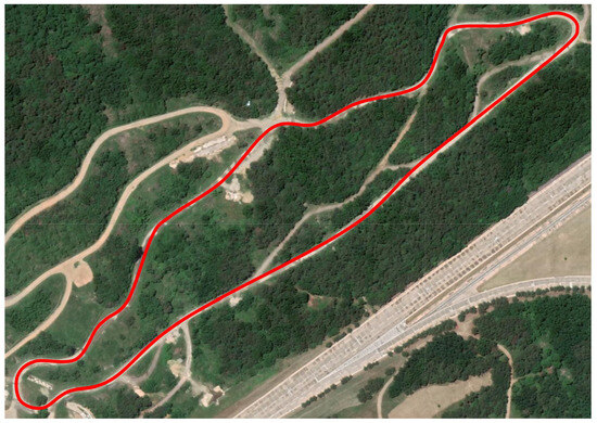
Figure 5. Proving ground for driving experiment. Red indicates the road the vehicle traveled on.

5.2. Results Analysis

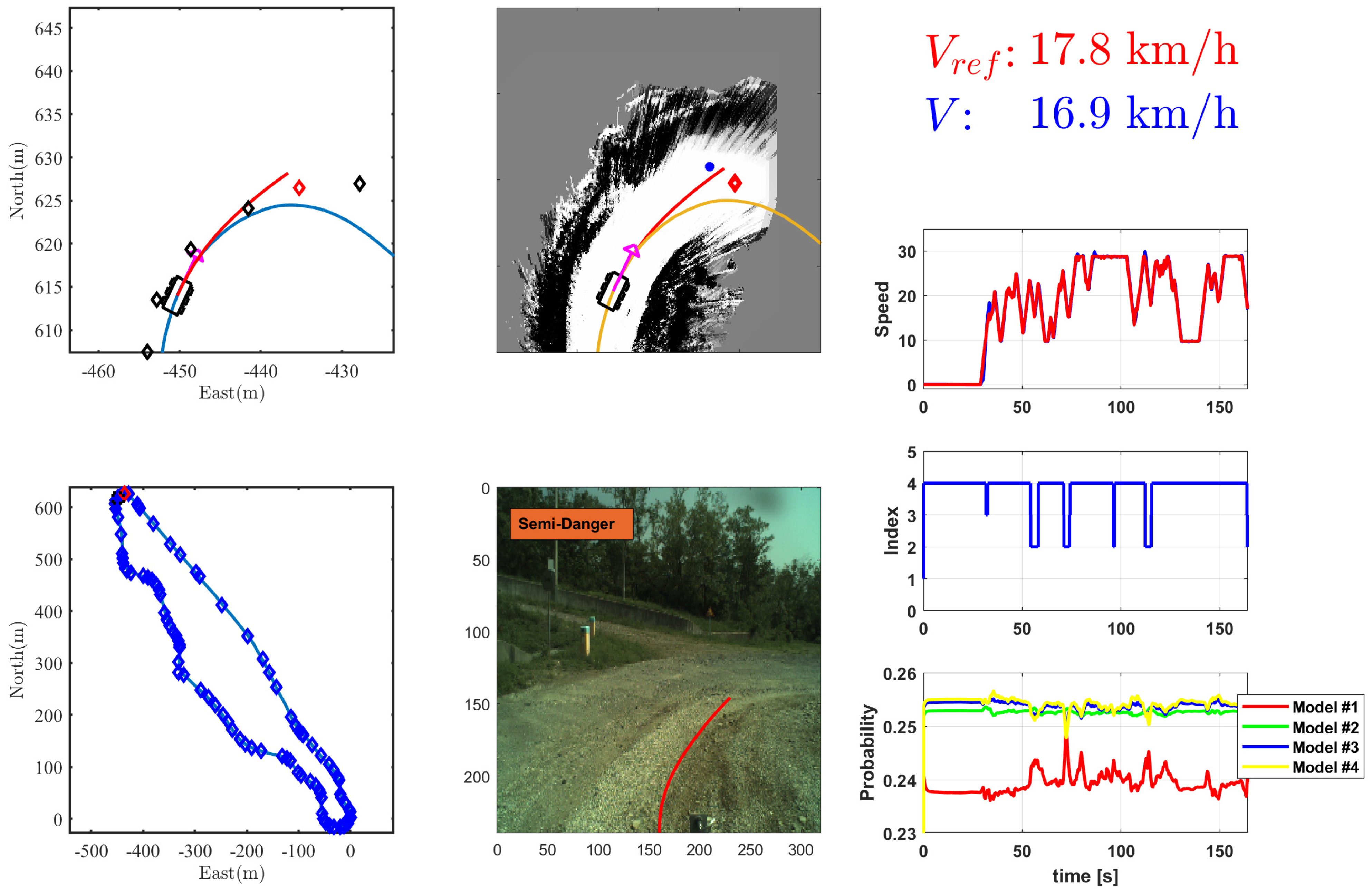
Figure 6 shows a snapshot of the abnormal driving area detection system using the proposed method. The lower-left subfigure shows the AGV’s current global position. The upper-left and middle subfigures show the local path planning result of the AGV to follow the global path. The upper-middle subfigure shows the probability map for the surrounding environment used for local path planning. The below-middle subfigure shows the front view obtained by the camera mounted on the AGV. The rest shows the AGV speed, the probability value of each model from IMM, and the index. The index is determined based on the output probability of the IMM and indicates the number of the model with the highest probability. Note that the AGV is slipping due to the severe bank angle of the unpaved road. To validate the proposed algorithm, we conducted the test for two cases.

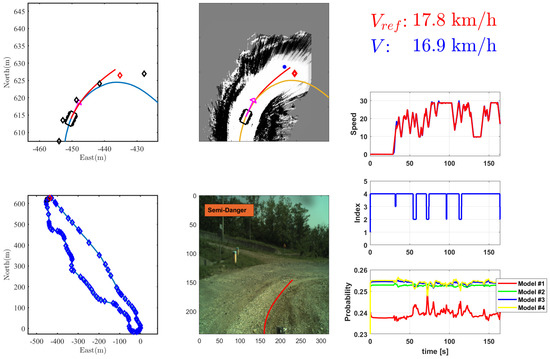
Figure 6. Snapshot of driving data of abnormal driving area detection system for AGV in Case 2.

• Case 1. Wet ground after rain, and worn tires.
• Case 2. Dry ground, and new tires.

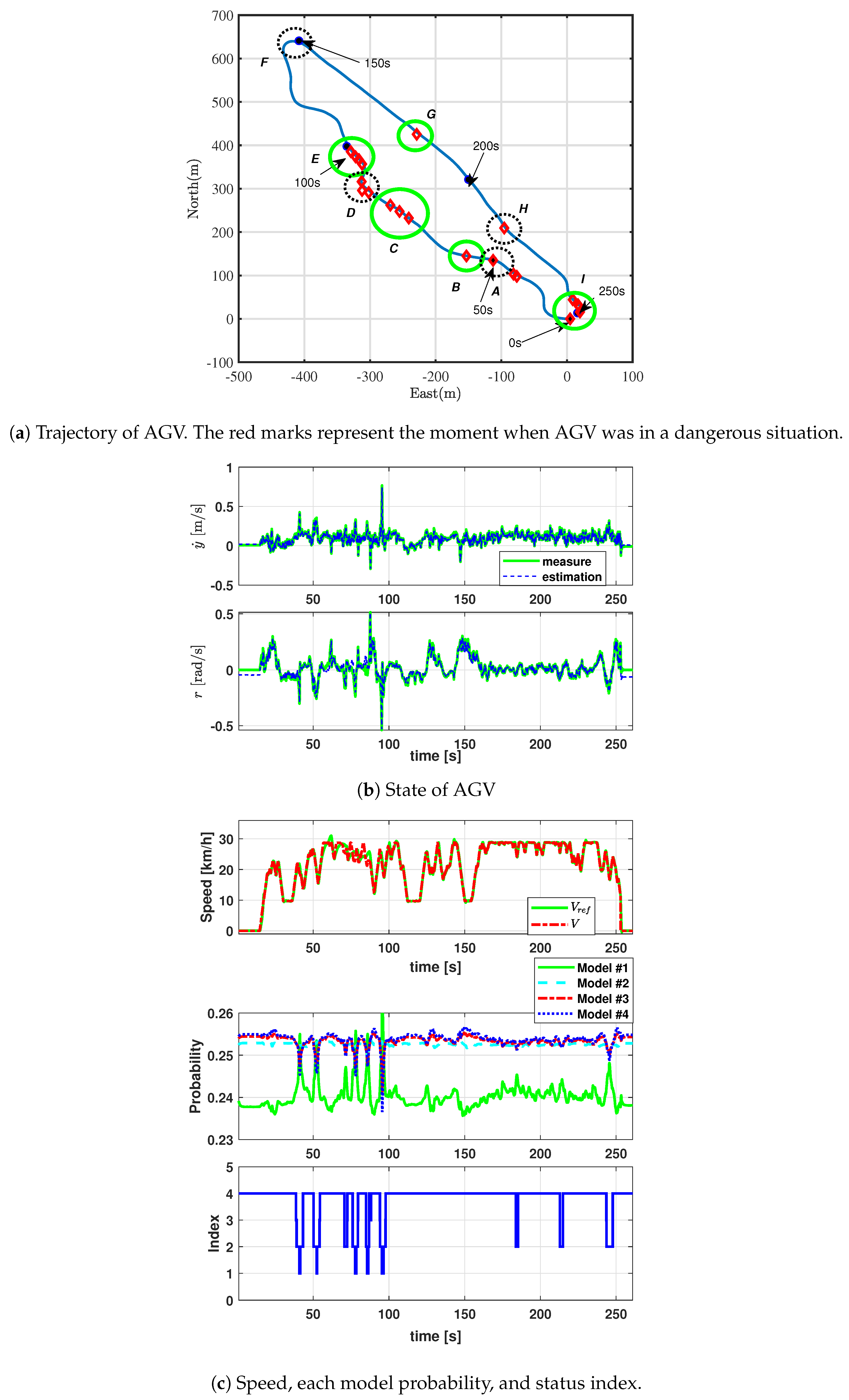
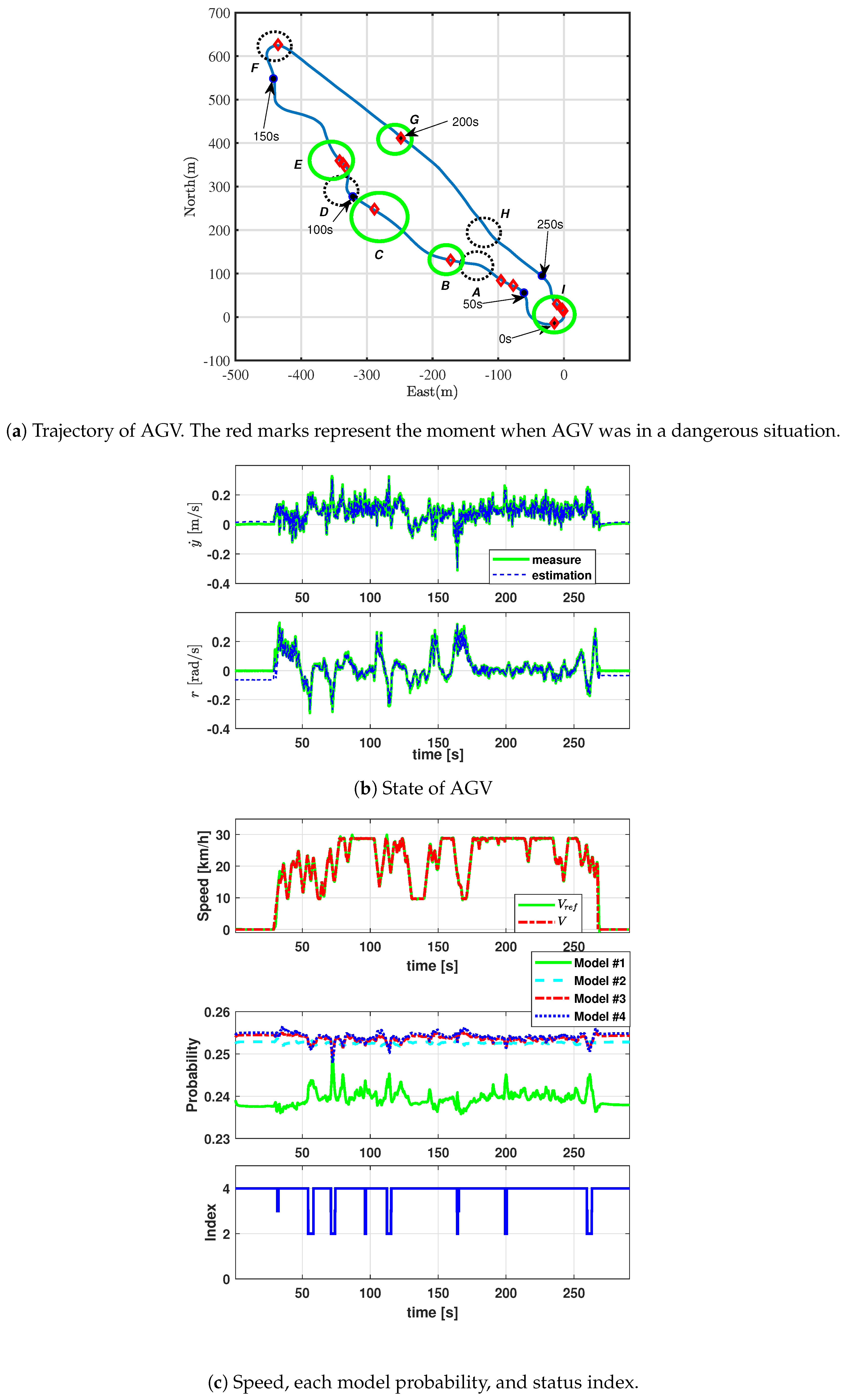
Experiments in these two cases allow us to identify the danger areas due to changes in tire–road friction. It is also possible to identify areas of danger that occur identically in both experiments as permanent areas of risk. Before we index the status of the AGV based on the probability values resulting from the interaction of multiple models, it can be confirmed that the proposed IMM filter can estimate the actual sensor value by showing reasonable performance as shown in Figure 7b and Figure 8b. Experiment results for both cases are represented in Figure 7 and Figure 8.

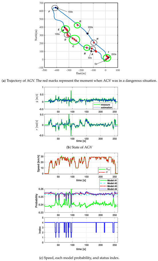
Figure 7. Case 1: wet ground after rain, and worn tires.

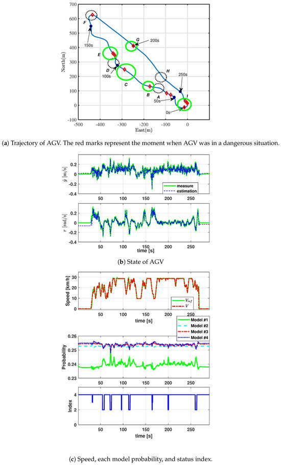
Figure 8. Case 2: dry ground, and new tires.

For comparison between the two cases, the areas showing the same pattern in the two tests are marked in a green circle, and the areas showing a different pattern are marked in a black circle as shown in Figure 7a and Figure 8a. The AGV was in a dangerous state in A, D, F, and H in Case 1, but it was not in Case 2. These sections have a greater curvature than other sections. In an autonomous path control algorithm, the target speed of the AGV is set to reach the maximum speed in consideration of the result of local path planning to complete the mission quickly. At this time, a normal driving condition is assumed, but if the frictional force between the tire and the road decreases, a slipping phenomenon occurs as shown in Case 1. As friction decreases, the speed must be reduced to maintain stability. But friction change is not taken into account in local path planning, sliding on curvy roads is inevitable. Area H is not very curvature, but since it is the point where the downhill road ends, it can be confirmed that slipping occurs in Case 1, where the frictional force between the road and the tire is low.

In both cases, AGV shows a dangerous status in B, C, E, G, and I. The test track consists of various types of unpaved roads, and the roads in sections B, C, and E are made up of small gravel. Therefore, the AGV did not take sufficient grip in both cases at these sections, so it caused a slip of AGV and a dangerous state appeared. Section G is a flat road that appears on the way downhill. In this section, the AGV shows a dangerous index in both cases because slip occurs due to inertia. In Section I, it can be observed that both cases are equally dangerous due to the severe curvature. The probabilities from interacting multiple models to identify the AGV status are shown in Figure 7c and Figure 8c. One can confirm that the probability of models 3 and 4 increases whenever the AGV slips for some reason such as longitudinal skidding or lateral sliding. One can also see that the index changes according to the highest probability value. Using the proposed algorithm, remote operators can monitor AGV danger status in real time. It is also possible to design control strategies based on driving conditions. Based on the driving status information of the reconnaissance AGV, additional strategies can be reorganized, such as selecting a different reconnaissance route and changing target speed.

6. Conclusions

In this research, we present the design scheme and experimental validation of an autonomous ground vehicle (AGV) abnormal driving area detection system using an interacting multiple model (IMM) filter. The dynamic behavior of the vehicle, which changes according to changes in the driving environment, was lumped into a parameter change of the system model. Using the probability of interacting multiple models, we can indirectly check the status of the vehicle in an unknown area. Also, it can help us detect abnormal behavior of the AGV such as skidding or sliding. Nine abnormal driving areas were discovered in the proving ground. In five of these areas, vehicles consistently exhibited abnormal driving behavior. The remaining four areas were confirmed to be affected by variables such as weather conditions and vehicle tire wear. As a result, using the proposed approach, the remote operator can directly decide whether to continue operating or not. Furthermore, additional strategies can be reorganized, such as selecting a different reconnaissance route and changing the target speed for the following AGV. The proposed method is simple but useful and meaningful for the remote operator compared to the image-only method. An operating strategy will be developed and a controller will be designed using this status index in future research.

References

- Shin, J.; Kwak, D.J.; Kim, J. Autonomous platooning of multiple ground vehicles in rough terrain. J. Field Robot. 2021, 38, 229–241. [Google Scholar] [CrossRef]
- Ni, J.; Hu, J.; Xiang, C. A review for design and dynamics control of unmanned ground vehicle. Proc. Inst. Mech. Eng. Part D J. Automob. Eng. 2021, 235, 1084–1100. [Google Scholar] [CrossRef]
- Grocholsky, B.; Keller, J.; Kumar, V.; Pappas, G. Cooperative air and ground surveillance. IEEE Robot. Autom. Mag. 2006, 13, 16–25. [Google Scholar] [CrossRef]
- Naranjo, J.E.; Jimenez, F.; Anguita, M.; Rivera, J.L. Automation kit for dual-mode military unmanned ground vehicle for surveillance missions. IEEE Intell. Transp. Syst. Mag. 2018, 12, 125–137. [Google Scholar] [CrossRef]
- Yang, Z.; Xiang, D.; Cheng, Y. VR panoramic technology in urban rail transit vehicle engineering simulation system. IEEE Access 2020, 8, 140673–140681. [Google Scholar] [CrossRef]
- Tikanmäki, A.; Bedrník, T.; Raveendran, R.; Röning, J. The remote operation and environment reconstruction of outdoor mobile robots using virtual reality. In Proceedings of the IEEE International Conference on Mechatronics and Automation (ICMA), Takamatsu, Japan, 6–9 August 2017; pp. 1526–1531. [Google Scholar]
- Jiang, C.; Hu, Z.; Mourelatos, Z.P.; Gorsich, D.; Jayakumar, P.; Fu, Y.; Majcher, M. R2-RRT*: Reliability-based robust mission planning of off-road autonomous ground vehicle under uncertain terrain environment. IEEE Trans. Autom. Sci. Eng. 2022, 19, 1030–1046. [Google Scholar] [CrossRef]
- Gao, H.; Cheng, B.; Wang, J.; Li, K.; Zhao, J.; Li, D. Object classification using CNN-Based fusion of vision and LIDAR in autonomous vehicle environment. IEEE Trans. Ind. Inform. 2018, 14, 4224–4231. [Google Scholar] [CrossRef]
- Dong, Z.; Wu, Y.; Pei, M.; Jia, Y. Vehicle type classification using a semisupervised convolutional neural network. IEEE Trans. Intell. Transp. Syst. 2015, 16, 2247–2256. [Google Scholar] [CrossRef]
- Sock, J.; Kim, J.; Min, J.; Kwak, K. Probabilistic traversability map generation using 3D-LIDAR and camera. In Proceedings of the IEEE International Conference on Robotics and Automation (ICRA), Stockholm, Sweden, 16–21 May 2016; pp. 5631–5637. [Google Scholar] [CrossRef]
- Wang, B.; Liu, Z.; Li, Q.; Prorok, A. Mobile robot path planning in dynamic environments through globally guided reinforcement learning. IEEE Robot. Autom. Lett. 2020, 5, 6932–6939. [Google Scholar] [CrossRef]
- Guo, H.; Shen, C.; Zhang, H.; Chen, H.; Jia, R. Simultaneous trajectory planning and tracking using an MPC method for cyber-physical systems: A case study of obstacle avoidance for an intelligent vehicle. IEEE Trans. Ind. Inform. 2018, 14, 4273–4283. [Google Scholar] [CrossRef]
- Ni, J.; Hu, J.; Xiang, C. Envelope control for four-wheel independently actuated autonomous ground vehicle through AFS/DYC integrated control. IEEE Trans. Veh. Technol. 2017, 66, 9712–9726. [Google Scholar] [CrossRef]
- Hwang, Y.; Kang, C.M.; Kim, W. Robust nonlinear control using barrier Lyapunov function under lateral offset error constraint for lateral control of autonomous vehicles. IEEE Trans. Intell. Transp. Syst. 2022, 23, 1565–1571. [Google Scholar] [CrossRef]
- Liang, J.; Tian, Q.; Feng, J.; Pi, D.; Yin, G. A polytopic model-based robust predictive control scheme for path tracking of autonomous vehicles. IEEE Trans. Intell. Veh. 2024, 9, 3928–3939. [Google Scholar] [CrossRef]
- Mazor, E.; Averbuch, A.; Bar-Shalom, Y.; Dayan, J. Interacting multiple model methods in target tracking: A survey. IEEE TRansactions Aerosp. Electron. Syst. 1998, 34, 103–123. [Google Scholar] [CrossRef]
- Blom, H.A.; Bar-Shalom, Y. The interacting multiple model algorithm for systems with markovian switching coefficients. IEEE Trans. Autom. Control 1988, 33, 780–783. [Google Scholar] [CrossRef]
- Li, X.R.; Jilkov, V.P. Survey of maneuvering target tracking. Part V. Multiple-model methods. IEEE Trans. Aerosp. Electron. Syst. 2005, 41, 1255–1321. [Google Scholar]
- Toledo-Moreo, R.; Zamora-Izquierdo, M.A.; Úbeda-Miñarro, B.; Gómez-Skarmeta, A.F. High-integrity IMM-EKF-based road vehicle navigation with low-cost GPS/SBAS/INS. IEEE Trans. Intell. Transp. Syst. 2007, 8, 491–511. [Google Scholar] [CrossRef]
- Kang, C.M.; Lee, S.-H.; Chung, C.C. Vehicle lateral motion estimation with its dynamic and kinematic models based interacting multiple model filter. In Proceedings of the IEEE Conference on Decision and Control, Las Vegas, NV, USA, 12–14 December 2016; pp. 2449–2454. [Google Scholar]
- Kong, J.; Pfeiffer, M.; Schildbach, G.; Borrelli, F. Kinematic and dynamic vehicle models for autonomous driving control design. In Proceedings of the IEEE Intelligent Vehicles Symposium, Seoul, Republic of Korea, 28 June–1 July 2015; pp. 1094–1099. [Google Scholar]
- Judalet, V.; Glaser, S.; Gruyer, D.; Mammar, S. IMM-based sensor fault detection and identification for a drive-by-wire vehicle. IFAC-PapersOnLine 2015, 48, 1158–1164. [Google Scholar] [CrossRef]
- Kim, B.; Yi, K.; Yoo, H.-J.; Chong, H.-J.; Ko, B. An IMM/EKF approach for enhanced multitarget state estimation for application to integrated risk management system. IEEE Trans. Veh. Technol. 2014, 64, 876–889. [Google Scholar] [CrossRef]
- Rajamani, R. Vehicle Dynamics and Control, 2nd ed.; Springer: Berlin/Heidelberg, Germany, 2012. [Google Scholar]
- Seah, C.E.; Hwang, I. Algorithm for performance analysis of the IMM algorithm. IEEE Trans. Onaerospace Electron. Syst. 2011, 47, 1114–1124. [Google Scholar] [CrossRef]
- Shin, J.; Kwak, D.; Kwak, K. Robust path control for an autonomous ground vehicle in rough terrain. Control Eng. Pract. 2020, 98, 104384. [Google Scholar] [CrossRef]
- Choi, J.-H.; Park, Y.-W.; Kim, J.; Choe, T.-S.; Song, J.-B. Federated filter based unmanned ground vehicle localization using 3D range registration with digital elevation model in outdoor environments. J. Field Robot. 2012, 29, 298–314. [Google Scholar] [CrossRef]
Disclaimer/Publisher’s Note: The statements, opinions and data contained in all publications are solely those of the individual author(s) and contributor(s) and not of MDPI and/or the editor(s). MDPI and/or the editor(s) disclaim responsibility for any injury to people or property resulting from any ideas, methods, instructions or products referred to in the content. |
© 2024 by the authors. Licensee MDPI, Basel, Switzerland. This article is an open access article distributed under the terms and conditions of the Creative Commons Attribution (CC BY) license (https://creativecommons.org/licenses/by/4.0/).