Enhancing Gearbox Fault Diagnosis through Advanced Feature Engineering and Data Segmentation Techniques

Abstract

Efficient gearbox fault diagnosis is crucial for the cost-effective maintenance and reliable operation of rotating machinery. Despite extensive research, effective fault diagnosis remains challenging due to the multitude of features available for classification. Traditional feature selection methods often fail to achieve optimal performance in fault classification tasks. This study introduces diverse ranking methods for selecting the relevant features and utilizes data segmentation techniques such as sliding, windowing, and bootstrapping to strengthen predictive model performance and scalability. A comparative analysis of these methods was conducted to identify the potential causes and future solutions. An evaluation of the impact of enhanced feature engineering and data segmentation on predictive maintenance in gearboxes revealed promising outcomes, with decision trees, SVM, and KNN models outperforming others. Additionally, within a fully connected network, windowing emerged as a more robust and efficient segmentation method compared to bootstrapping. Further research is necessary to assess the performance of these techniques across diverse datasets and applications, offering comprehensive insights for future studies in fault diagnosis and predictive maintenance.

1. Introduction

Gearboxes and rotating machinery are crucial across many industries for their adaptability to torque and speed requirements [1]. In wind turbine systems, gearboxes require regular maintenance to ensure operational safety and reliability. Gearbox maintenance is time-intensive with an average of 256 h, with 59% of system failures attributed to gearbox malfunctions [2]. Factors contributing to these failures include transportation issues, misalignment, tool surface irregularities, overloading, and design/manufacturing errors [3]. Studies detail wind turbine sub-assembly failure rates, with reports of 60 days of annual downtime due to gearbox faults impacting system efficiency and productivity.

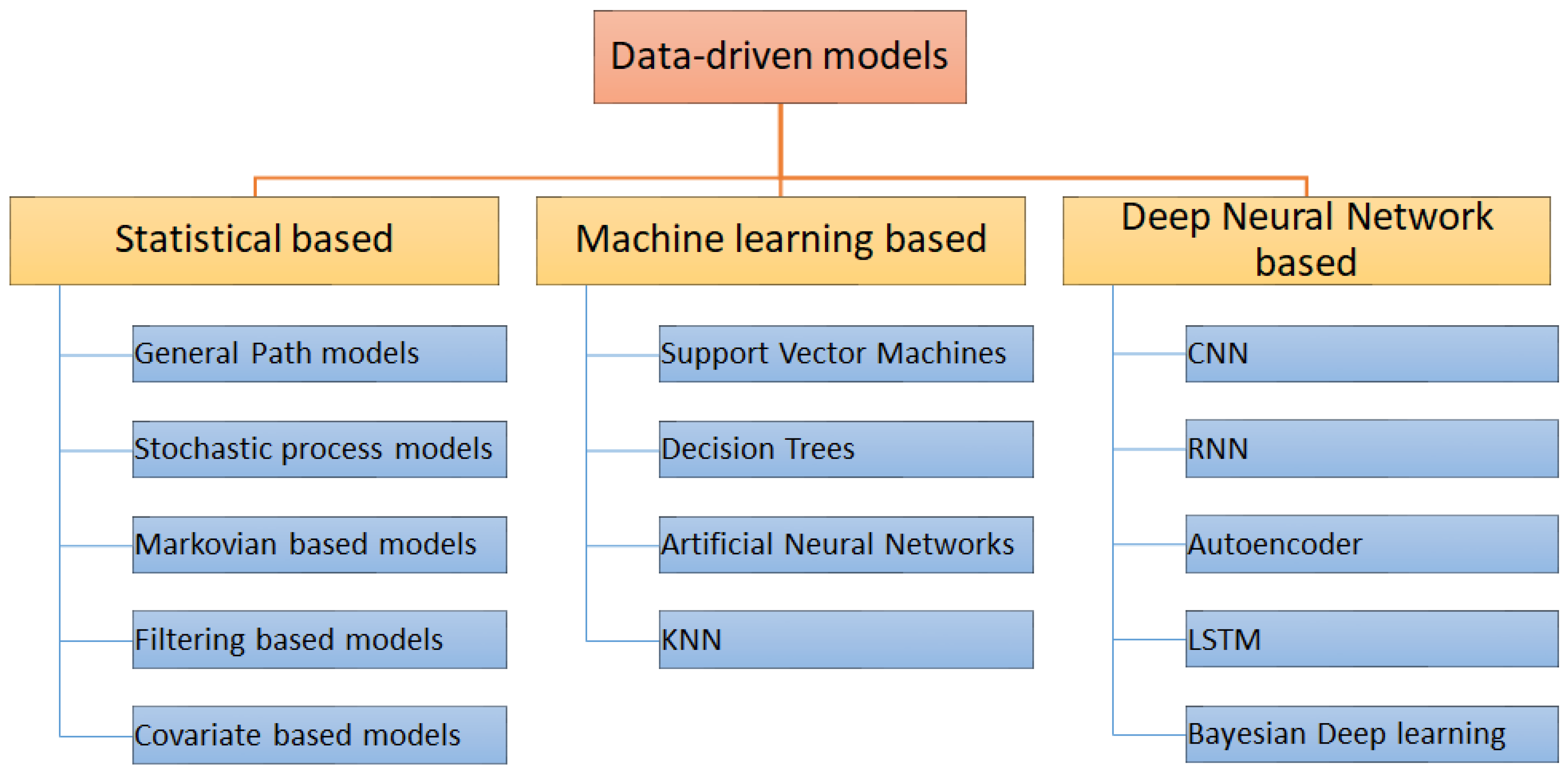
Predictive maintenance, an advanced form of condition-based monitoring, predicts machine failures by analyzing system health data collected through methods like vibration analysis, thermography, visual inspection, and tribology [4]. Vibration monitoring is particularly favored due to its prevalence in stationary machines, allowing for the identification of undesirable patterns indicative of failure states. With the advancement of technology, intelligent diagnostic systems, notably artificial intelligence (AI) and deep learning methods, have gained prominence for their ability to learn from raw data. Statistical models, conventional machine learning, and deep neural networks are often utilized in data-driven prognostics for predictive maintenance objectives, as depicted in Figure 1.

Figure 1. Overview of data-driven prognostic models.

In gearbox predictive maintenance, feature engineering is essential for optimizing predictive models by selecting and constructing the relevant features from raw sensor data. Various techniques can be employed, including statistical features to capture fundamental behavior, time-domain features for degradation patterns, frequency-domain features for gear faults, amplitude modulation features for gear faults, waveform features for signal morphology, time-frequency features for simultaneous time and frequency information, and trend analysis features for long-term degradation trends [5]. Feature selection is crucial for enhancing model performance and interpretability. Filter methods like correlation analysis or information gain, wrapper methods like recursive feature elimination or genetic algorithms, and embedded methods like L1 regularization or tree-based feature importance aid in selecting key features, contributing to dimensionality reduction, noise mitigation, and improved model accuracy [6].

Moreover, feature selection contributes to enhancing model performance and generalization, thereby mitigating the risk of overfitting [7]. The inclusion of irrelevant or noisy features in the model can result in decreased prediction accuracy and increased complexity. Feature selection addresses this concern by identifying the most relevant features directly influencing the predictive task. By prioritizing the most informative features, the model gains robustness and becomes better equipped to capture the underlying patterns and relationships associated with gearbox failures. Additionally, feature selection enhances the interpretability and comprehension of predictive models. Identification of the most influential features offers insights into the primary factors contributing to gearbox failures. This knowledge aids domain experts in comprehending the root causes of failures and optimizing maintenance strategies, facilitating informed decision-making processes [8]. By selecting a concise set of features, feature selection facilitates improved interpretation of the results, enabling stakeholders to gain a better understanding of gearbox health and the factors driving degradation.

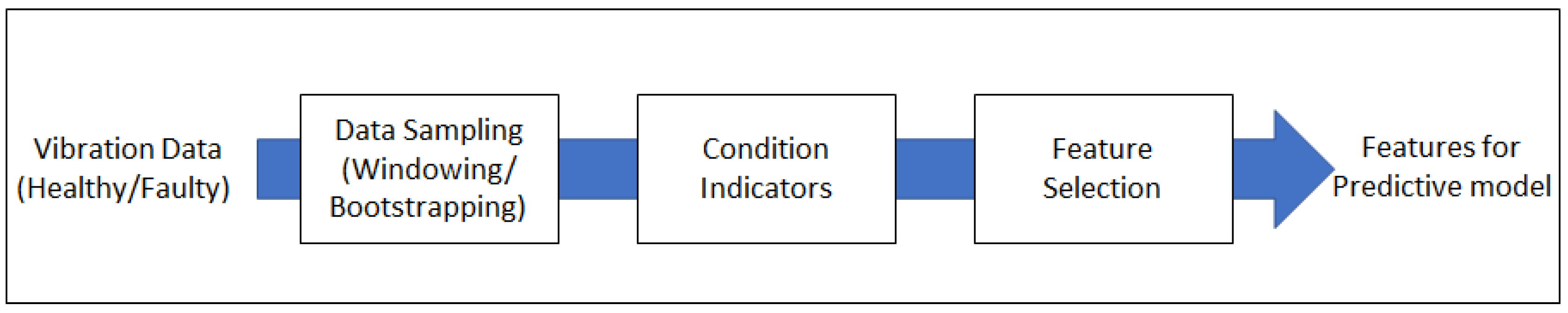
This study focuses on the multifaceted aspects of feature selection processes aimed at reducing data dimensionality by identifying a subset of relevant features. This dimensionality reduction serves to enhance computational efficiency and alleviate the challenges associated with the “curse of dimensionality”, particularly pertinent in high-dimensional datasets. By eliminating extraneous features, feature selection concentrates the model’s attention on the most informative aspects of the data, facilitating more effective detection of gearbox faults. Two datasets from distinct gearboxes were utilized for this research. The first dataset delineated the processes of feature engineering and ranking selection, while the second dataset served for validation purposes. Figure 2 provides an overview of the defined processes for this research. Initially, vibration data from the first dataset underwent pre-processing to convert it into a time-series format. The data was then classified into three categories: raw data without segmentation, data processed through windowing, and data processed through bootstrapping. Subsequently, time-domain features were extracted using different condition indicators. Feature selection was performed at the concluding stage, wherein a limited set of features were chosen for enhanced execution. Various feature ranking methods were employed to facilitate this selection process. Following feature engineering, the data was analyzed to comprehend the impact of applied transformations on its patterns, relationships, and suitability for machine learning (ML) models. This ensured that the engineered features align with the objectives and augment predictive performance. The selected features were subsequently used as input into various machine learning classification models to determine the optimal models for predictive purposes. The primary motivation for this research lies in enhancing feature engineering processes, particularly focusing on feature selection, to achieve optimal outcomes for predictive models.

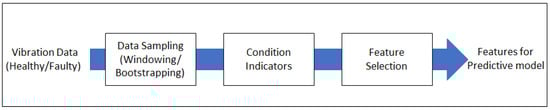
Figure 2. Data processing steps used in the current study.

2. Dataset and Methodologies

2.1. Dataset Processing

An open-source, publicly available gearbox dataset was used for the study [2]. The data was sourced from SpectraQuest’s Gearbox Fault Diagnostics Simulator (https://data.world/gearbox/gear-box-fault-diagnosis-data-set) (accessed on 28 November 2022). This dataset comprised both healthy and faulty vibration data obtained from a malfunctioning gearbox operating under varying load conditions (ranging from 0% to 90%) at a constant rotational speed of 30 Hz. Figure 3 presents the vibration measurements of a single channel of this gearbox dataset [2].

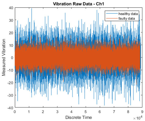
Figure 3. Raw data of vibration measurements of a single channel of this gearbox dataset as obtained from SpectraQuest’s Gearbox Fault Diagnostics Simulator.

2.2. Data Segmentation

Segmentation of data is a crucial step in facilitating effective analysis and training of machine learning models [9]. It involves dividing the dataset into distinct subsets or segments. Three main types of segmentation viz. temporal, spatial, and categorical were explored in this study. Temporal segmentation involved partitioning the data based on time aspects, ensuring that samples from different time periods were separated [9]. This is particularly useful for time series analysis and forecasting. Spatial segmentation partitioned the data based on geographical or spatial attributes [10]. Categorical segmentation divided the data based on discrete categories or classes [11]. To ensure the reliability, the resulting segments were evaluated and validated using techniques such as cross-validation [12].

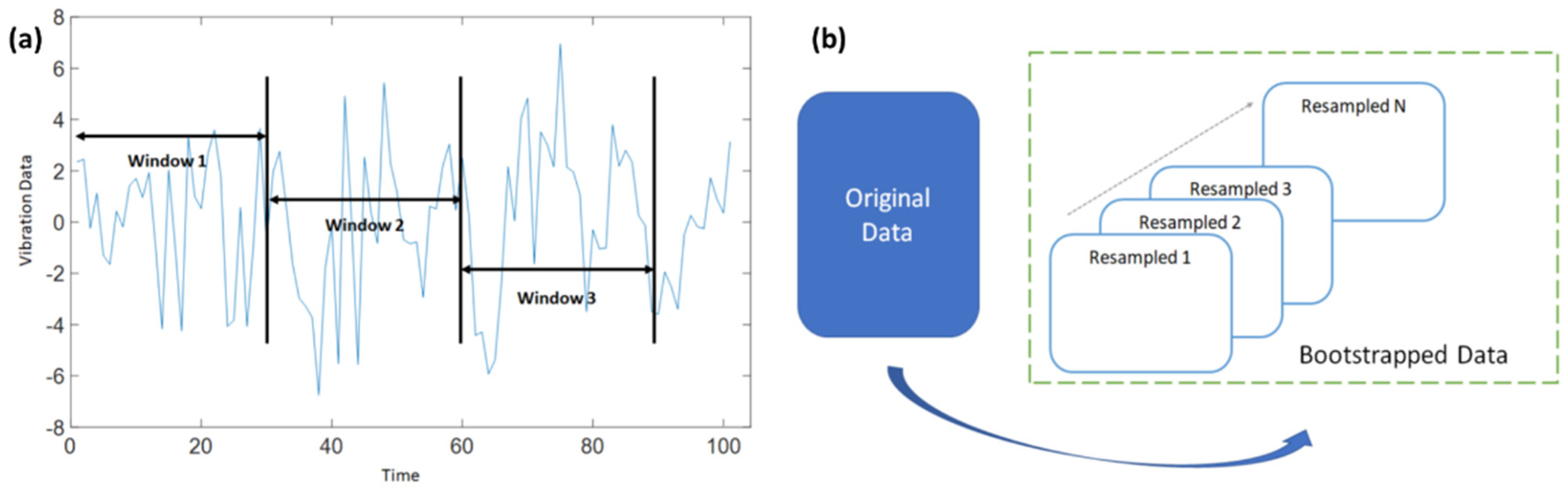
In addition to traditional segmentation methods, sliding window techniques were employed for data stream analysis. Specifically, fixed-length non-overlapping sliding windows (FNSW) and fixed-length overlapping sliding windows (FOSW) were used [13]. FNSW was used to partition the data into equal-sized independent segments, while FOSW involved sharing some data segments to ensure a higher temporal resolution [14]. To address constraints arising from data availability, bootstrapping was employed as a resampling technique [15]. It involved creating multiple subsets from the original dataset by random sampling with replacements. Twenty datasets were derived through experimental procedures. A sample extracted from each dataset underwent comparative analysis with the sample data originating from the original dataset. Subsequently, only those datasets demonstrating a proximal relationship between their sample mean and the mean of the original dataset were considered for progression in the analysis. Models trained on these subsets were then evaluated for stability and uncertainty. For this study, the following segmentation was carried out for the original dataset:

• Windowing: windowing size was 10 and the original dataset was sequenced to 10-fold;
• Bootstrapping: resampling size was 10 and the new data was resampled to 10-fold;
• Figure 4a,b describe the windowing (FNSW) and bootstrapping techniques, respectively, employed for this study. The algorithm used for this research is described in Algorithm 1.
  

  Figure 4. (a) Data segmentation with windowing, (b) data segmentation with bootstrapping.

Algorithm 1. Calculate y = bootstrap(x,N)

Require: x > 0∧N ≥ 1 where x is Input data, N is bootstrap resamples Ensure: y = bootstrap(x,N) 1: if N < 1 then 2:   N ⇐1 3: end if 4: if x < 1 then 5:   print(Input data is insufficient) 6: end if 7: S⇐ size(x) 8: if S == 1 then 9:   Out ⇐X(rand{S,N}) 10: end if

2.3. Condition Indicators

Vibration analysis is a widely used technique for predictive maintenance. In this study, time-based analysis was used, which involved statistical measurement techniques for feature extraction from the vibration signals obtained from the gearbox [16]. These features served as condition indicators, providing information about the health status of the gearbox. The condition indicators employed in this study included the following:

• Root mean square (RMS) quantifies the vibration amplitude and energy of a signal in the time domain. It is computed as the square root of the average of the sum of squares of signal samples, expressed as:

  $$RM{S}_x=\sqrt{\frac{1}{N}\left[{{\displaystyle \sum }}_{i=1}^N{\left(x_i\right)}^2\right]}$$

  (1)

  where x denotes the original sampled time signal, N is the number of samples, and i is the sample index.
• Standard deviation (STD) indicates the deviation from the mean value of a signal, calculated as:

  $$STD=\sqrt{\frac{1}{N-1}}{{\displaystyle \sum }}_{i=1}^N{\left(x_i-\overline{x}\right)}^2$$

  (2)

  where x_i (i = 1, …, N) is the i-th sample point of the signal x, and $\overline{x}$ is the mean of the signal.
• Crest Factor (CF) represents the ratio of the maximum positive peak value of signal x to its rms_x value. It is devised to boost the presence of a small number of high-amplitude peaks, such as those caused by some types of local tooth damage. It serves to emphasize high-amplitude peaks, such as those indicating local tooth damage. A sine wave has a CF of 1.414. It is given by the following equation:

  $$\mathrm{CF}=\frac{x_0-pk}{rm{s}_x}$$

  (3)

  where pk denotes the sample for the maximum positive peak of the signal, and x₀ − pk is the value of x at pk.
• Kurtosis (K) measures the fourth-order normalized moment of a given signal x, reflecting its peakedness, i.e., the number and amplitude of peaks present in the signal. A signal comprising solely Gaussian-distributed noise yields a kurtosis value of 3. It is given by:

  $$K=\frac{\sqrt{N{{\displaystyle \sum }}_{i=1}^N{\left(x_i-\overline{x}\right)}^4}}{{\left({{\displaystyle \sum }}_{i=1}^N{\left(x_i-\overline{x}\right)}^2\right)}^2}$$

  (4)
• Shape factor (SF) characterizes the time series distribution of a signal in the time domain:

  $$SF=\frac{\sqrt{\frac{1}{N}\left[{{\displaystyle \sum }}_{i=1}^N{\left(x_i\right)}^2\right]}}{\sqrt{\frac{1}{N}\left[{{\displaystyle \sum }}_{i=1}^N{\left|x_i\right|}^2\right]}}$$

  (5)
• Skewness assesses the symmetry of the probability density function (PDF) of a time series’ amplitude. A time series with an equal number of large and small amplitude values has zero skewness, calculated as:

  $$Skewness=\frac{N{{\displaystyle \sum }}_{i=1}^N{\left(x_i-\overline{x}\right)}^3}{{\left\{\sqrt{{{\displaystyle \sum }}_{i=1}^N{\left(x_i-\overline{x}\right)}^2}\right\}}^3}$$

  (6)
• Clearance factor indicates the symmetry of the PDF of a time series’ amplitude, given by:

  $$CF=\frac{\max \left|x_i\right|}{\frac{1}{N}\left[{{\displaystyle \sum }}_{i=1}^N\sqrt{{\left|x_i\right|}^2}\right]}$$

  (7)
• Impulse factor denotes the symmetry of the probability density function (PDF) of a time series’ amplitude, calculated as:

  $$IF=\frac{\max \left|x_i\right|}{\frac{1}{N}\left[{{\displaystyle \sum }}_{i=1}^N\left|x_i\right|\right]}$$

  (8)
• Signal-to-noise ratio (SNR) represents the ratio of the useful signal, such as desired mechanical power or motion, to unwanted noise and vibrations generated within a gearbox during operation. It is expressed as:

  $$SNR=101lo{g}_{10}\left(\frac{P_{signal}}{P_{noise}}\right)$$

  (9)

  where P is the amplitude in dB.
• Signal-to-noise and distortion ratio (SINAD) measures signal quality in electronics, comparing the desired signal power to the combined power of noise and distortion components:

  $$SINAD=101lo{g}_{10}\left(\frac{P_{signal}}{P_{signal}+P_{distortion}}\right)$$

  (10)

  where P is the amplitude in dB.
• Total harmonic distortion (THD) assesses how accurately a vibration system reproduces the output signal from a source.
• Mean represents the average of the sum of squares of signal samples.
• Peak value denotes the maximum value of signal samples.

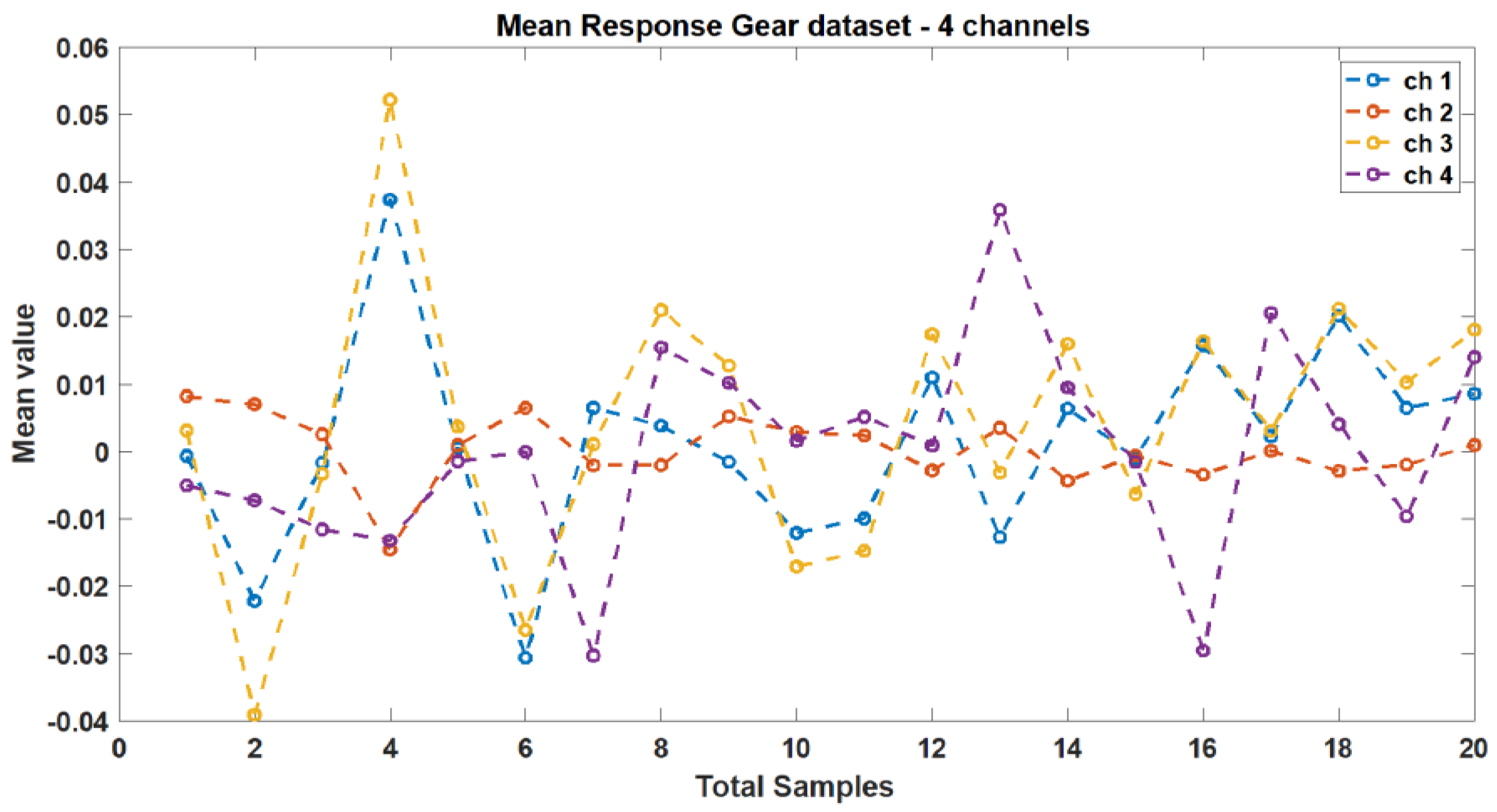
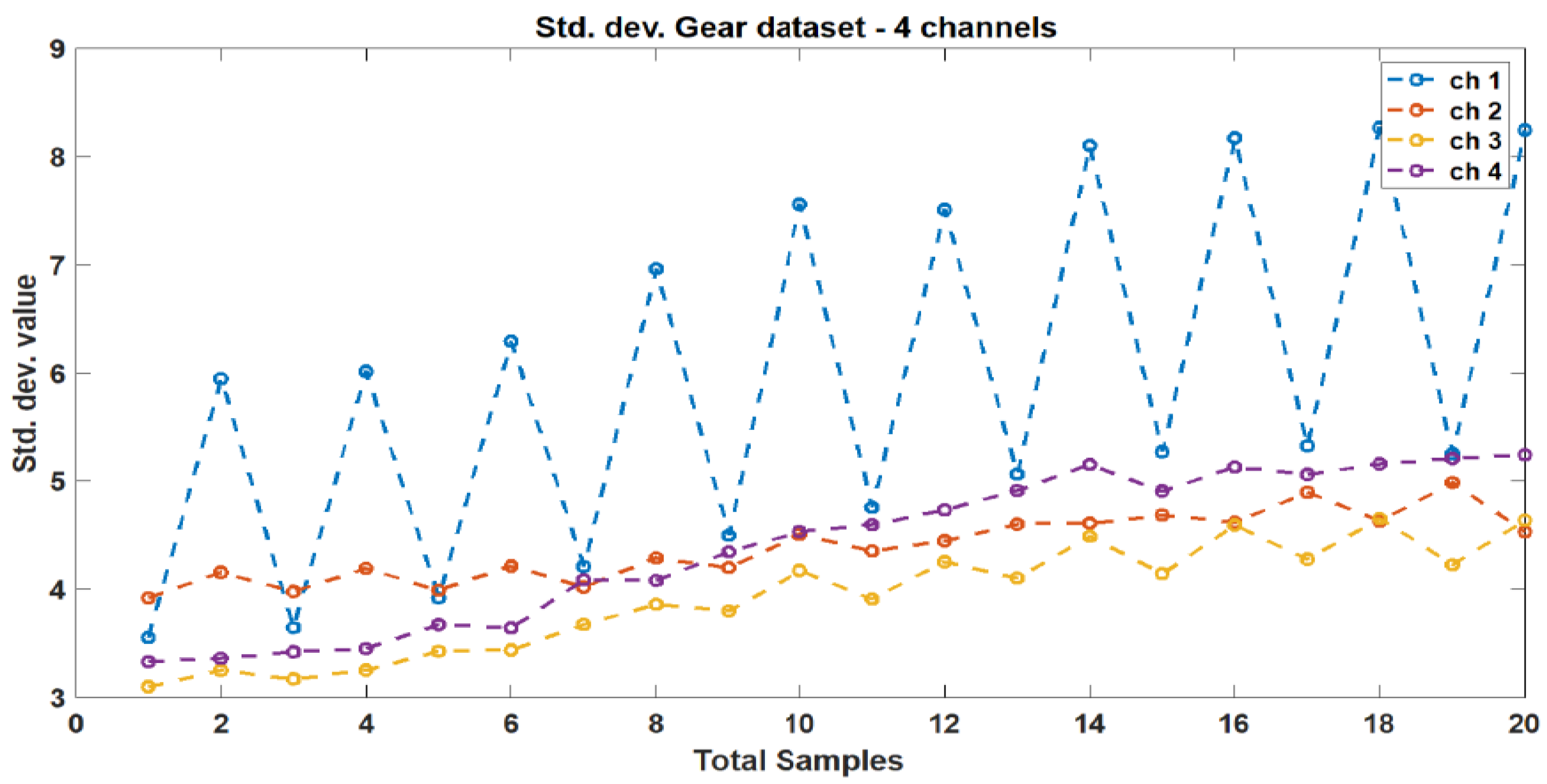
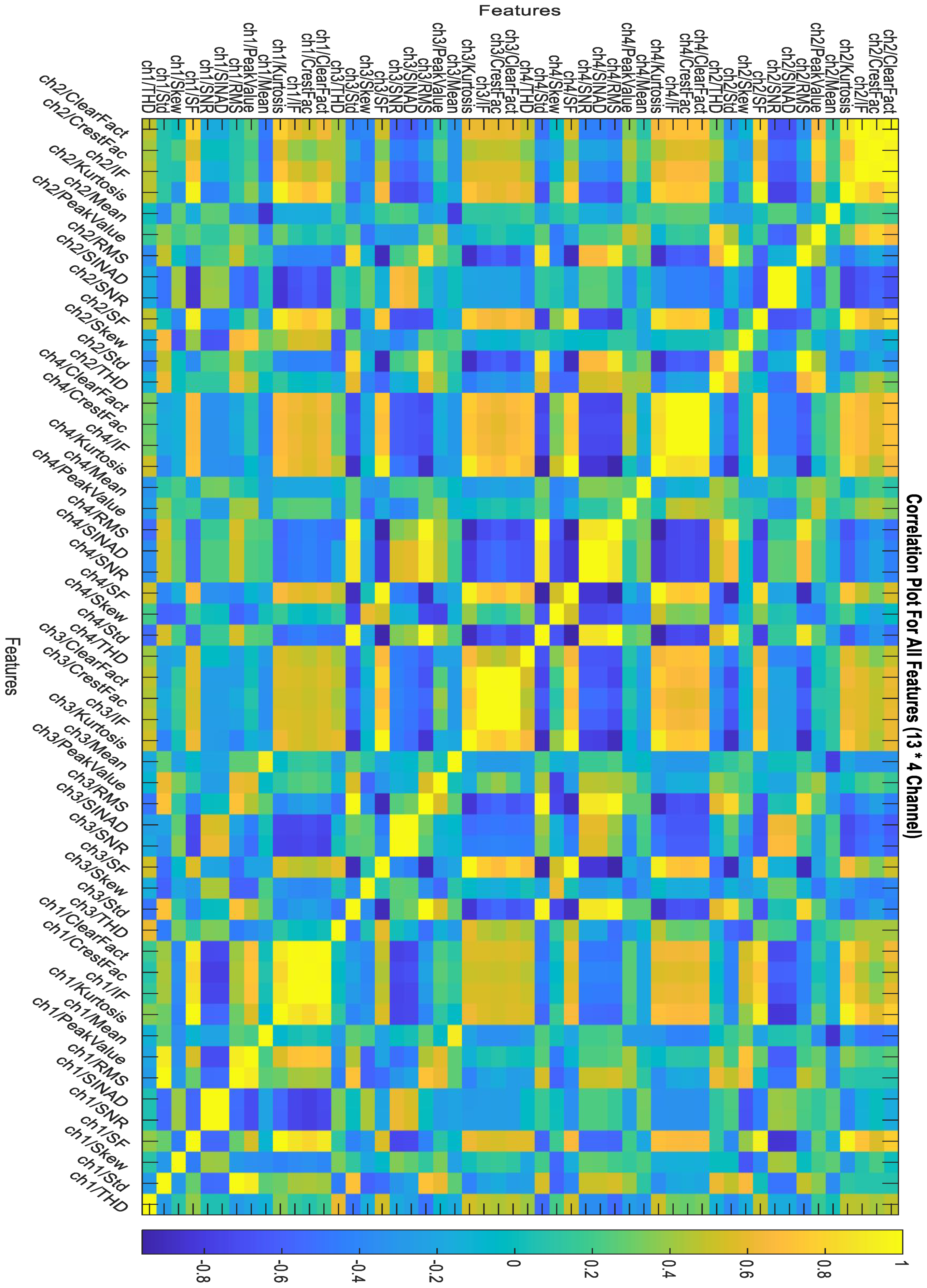
These indicators were selected based on their ability to capture relevant information about the vibration signals and their potential to identify faults in the gearbox. The mean and standard deviation responses from the original dataset’s four channels are depicted in Figure 5 and Figure 6, respectively. Figure 7 illustrates the correlation plot for all features extracted via condition indicators without data segmentation.

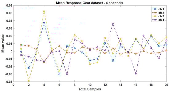
Figure 5. Mean response between different vibration data.

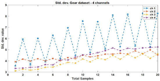
Figure 6. Standard deviation response between different vibration data.

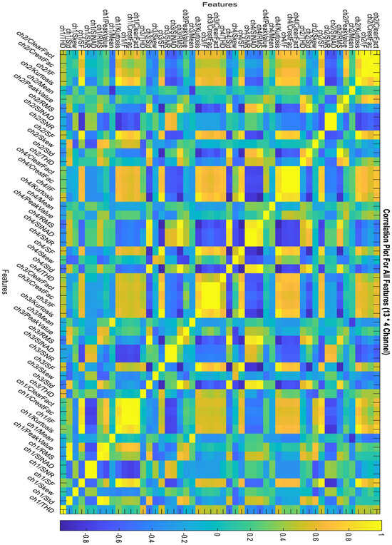
Figure 7. Correlation plot for all features without data segmentation.

2.4. Feature Ranking and Selection

Feature ranking is a critical step in data analysis and machine learning as it helps identify the most informative features for a given task. In this study, various feature ranking methods were employed to assess the relevance and discriminatory power of the features. These methods allowed the study to rank the features based on their ability to contribute to the predictive task and identify the most relevant features for further analysis. The methods are described as below:

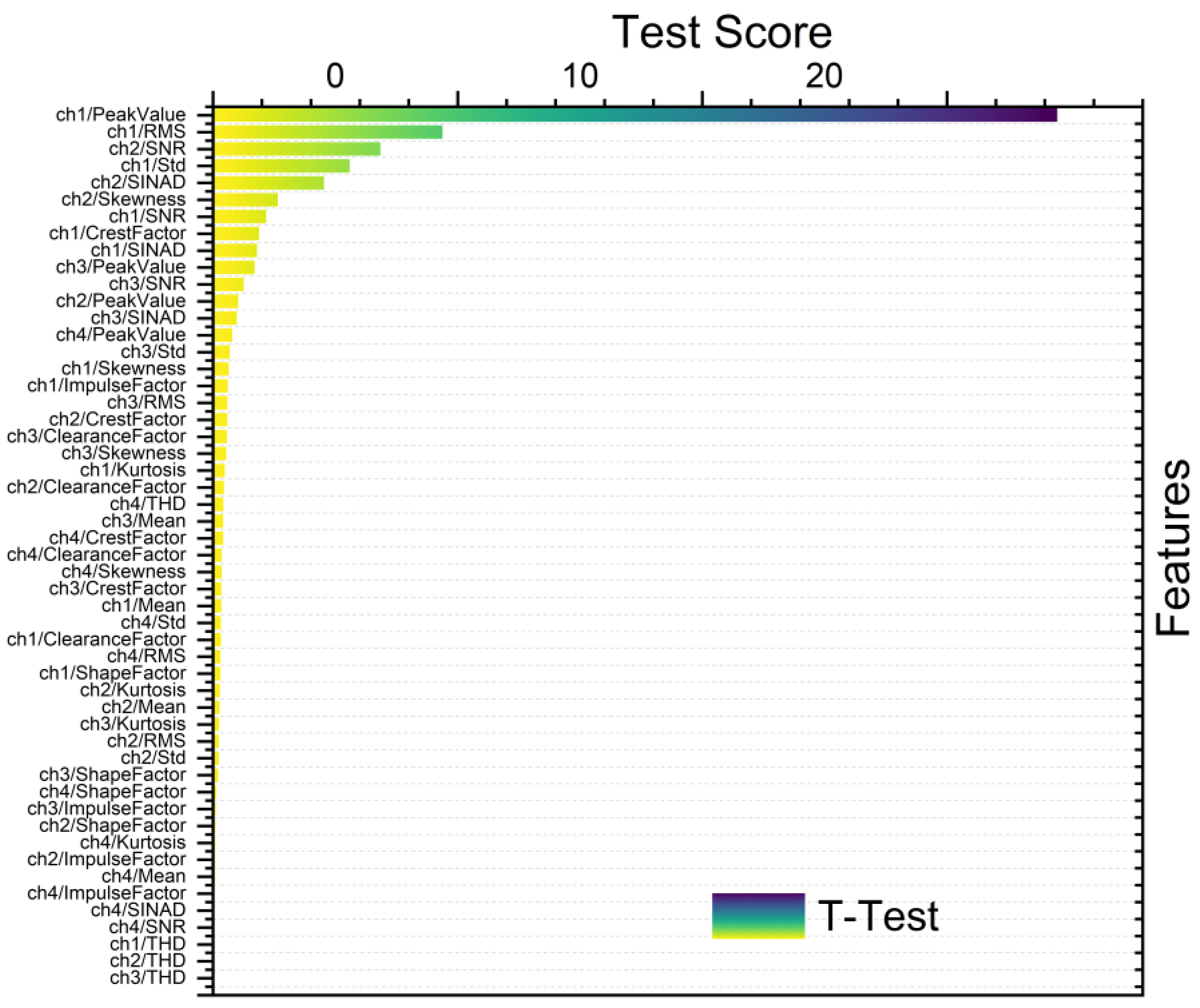
• T-test is generally employed to discern statistically significant differences between the means of two groups. Herein, it was applied in feature ranking to compare feature means across distinct classes or groups. Features exhibiting significant differences in means are identified as relevant for discrimination purposes [17].
• ROC analysis serves as a pivotal method for assessing the efficacy of classification models. Within the context of feature ranking, the ROC curve is utilized to evaluate the trade-offs between true positive rates and false positive rates at varying feature thresholds. Features characterized by a higher area under the ROC curve (AUC) are indicative of superior discriminatory power and are consequently ranked higher [18].
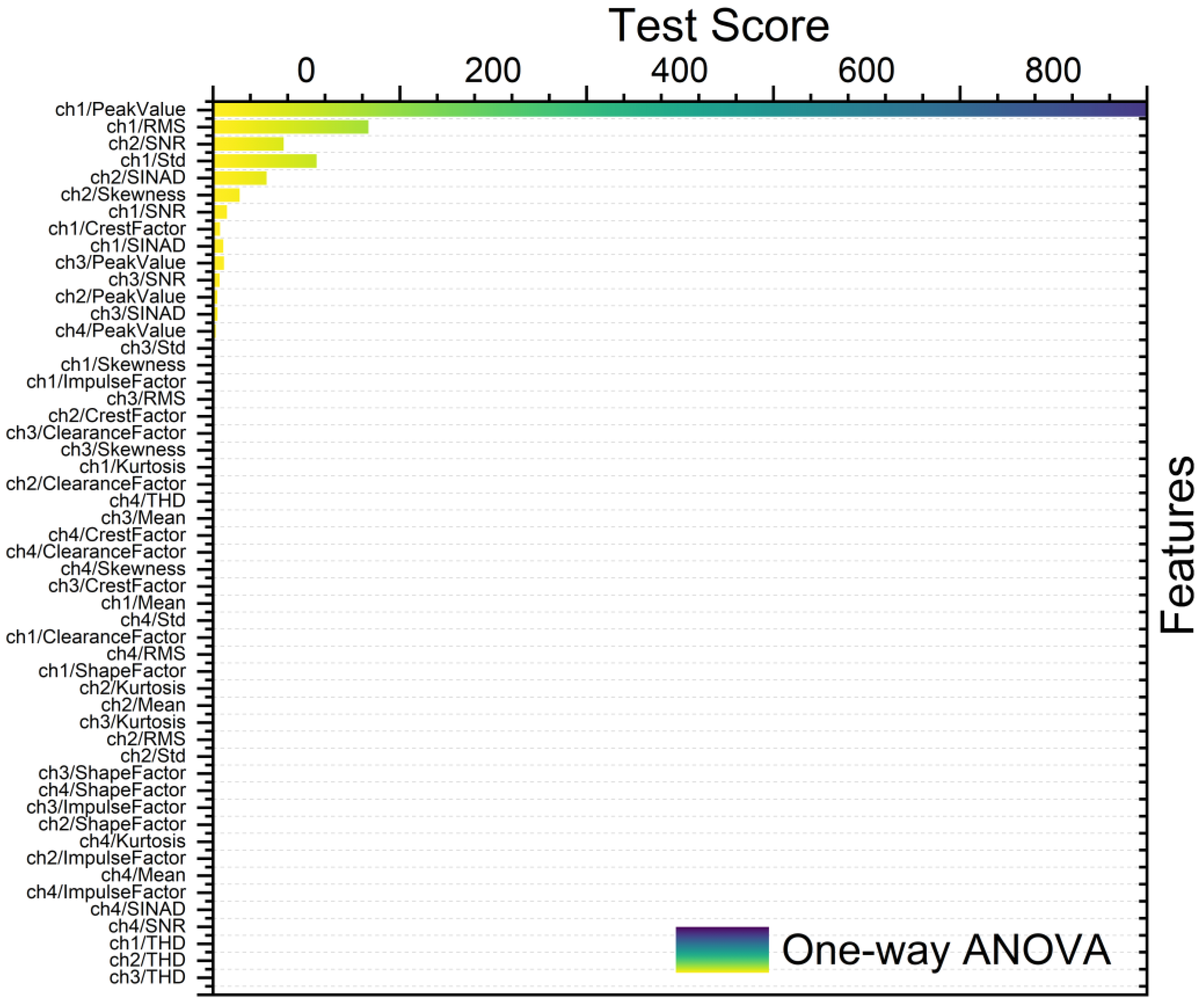
• One-way analysis of variance (ANOVA) method is used to compare means across three or more groups. Herein, one-way ANOVA served for feature ranking to ascertain the significance of variation in feature values across different classes or groups. Features demonstrating noteworthy differences in means between groups are deemed pertinent for discrimination [19].
• Monotonicity, denoting the relationship between a feature and its target variable, is evaluated using Spearman’s rank correlation coefficient. Features exhibiting monotonic relationships with the target variable are considered informative for the study’s objectives [20].
• Entropy, which serves as a measure of dataset disorder or uncertainty, plays a crucial role in feature ranking. Features characterized by higher entropy values signify greater variability and information content. To rank features based on their predictive utility, entropy-based methods such as information gain and mutual information are employed.
• Kruskal–Wallis test is a non-parametric statistical test which is utilized to compare medians across three or more groups. In feature ranking, this test is instrumental in assessing the significance of feature variations across different classes or groups. Features demonstrating significant median differences are identified as essential for discrimination [21].
• Variance-based unsupervised ranking was used to evaluate feature variability. Features exhibiting high variance values are indicative of greater diversity and are thus considered more informative for clustering or unsupervised learning tasks [22].
• Bhattacharyya distance is a metric quantifying the dissimilarity between probability distributions and is utilized to assess feature discriminative power. Larger Bhattacharyya distances between feature value distributions across classes indicate greater separability, thus highlighting the importance of features for classification purposes [23].

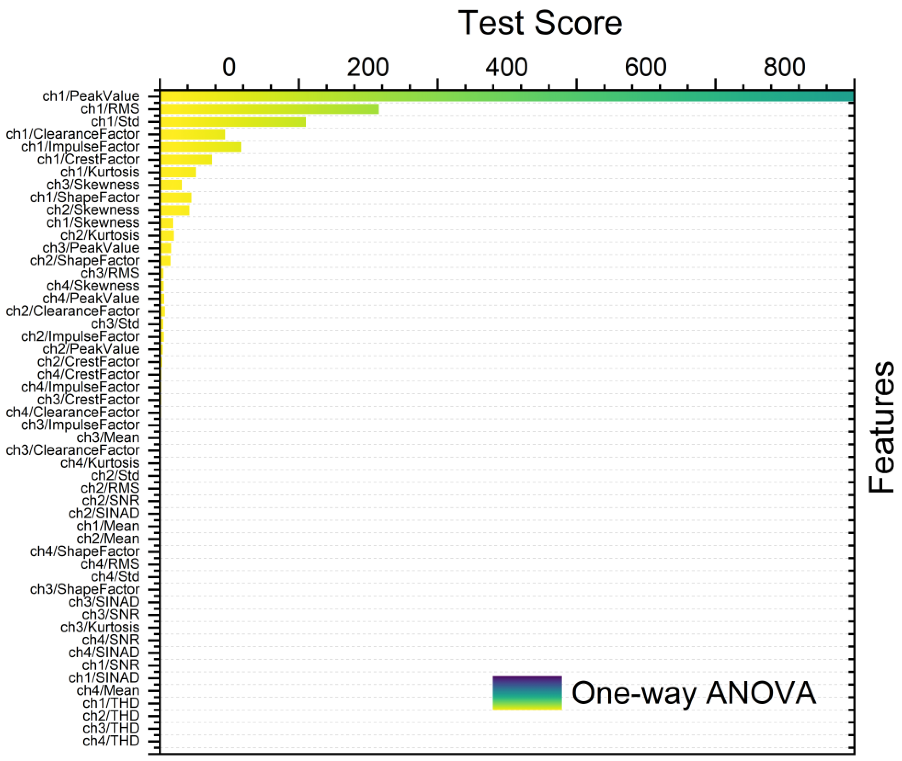
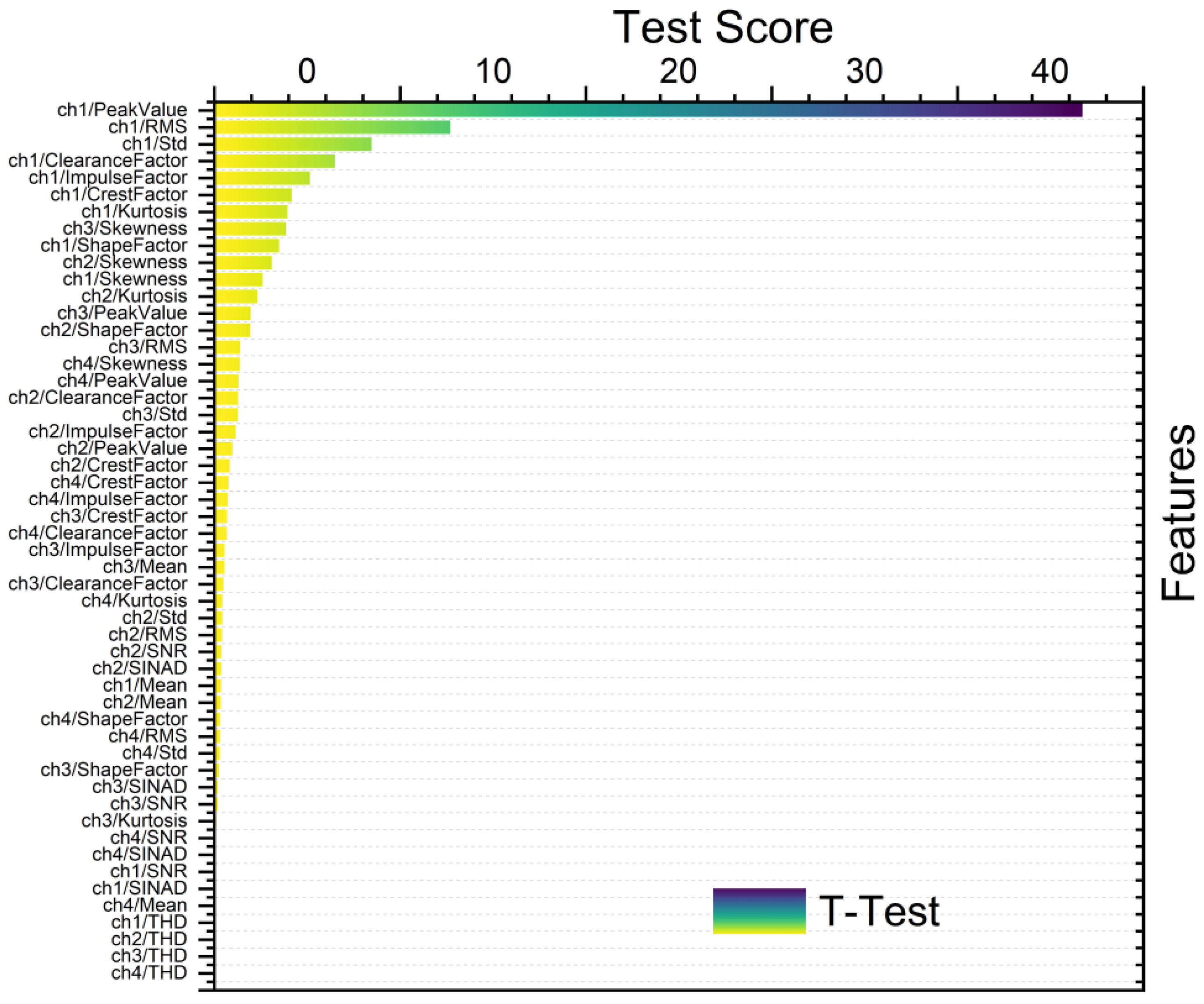
Figure 8, Figure 9, Figure 10 and Figure 11 show different feature rankings with one-way ANOVA and t-test with windowing and bootstrapping, respectively.

Figure 8. Ranking metric with one-way ANOVA with windowing.

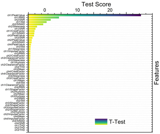
Figure 9. Ranking metric with t-test with windowing.

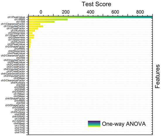
Figure 10. Ranking metric with one-way ANOVA with bootstrapping.

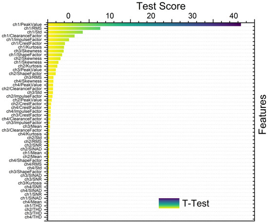
Figure 11. Ranking metric with t-test with bootstrapping.

The significance of correlation values ranging from 0 to 1 in ranking selection was also examined. A correlation of 0 signified the absence of a linear relationship between variables, indicating the importance of considering alternative factors for ranking decisions. Conversely, a correlation of 1 indicates a perfect positive relationship, indicating strong evidence of consistent association between variables [24]. For the current research, a correlation importance of 1 was adopted to ensure a consistent association with each feature and maximize the significance of correlation in the analysis.

Normalizing schemes are crucial preprocessing steps in feature selection. The choice of normalization scheme depends on the specific requirements of the feature selection algorithm and the characteristics of the data. Normalization ensures that different features are brought to a similar scale, facilitating faster convergence of algorithms and preventing certain features from overshadowing others [25]. Among the normalization schemes, such as min-max, softmax-mean-var, and none, min-max normalization is preferred due to its ability to maintain data relationships, aid interpretation, ensure fair treatment of algorithms, expedite convergence, and offer resistance to outliers [26]. The formula for min-max normalization is shown below:

$$X_{normalized}=\frac{X-X_{min}}{X_{max}-X_{min}}$$

(11)

Min-max normalization, also referred to as feature scaling, scales the data to a fixed range, typically between 0 and 1, using the minimum and maximum values of the data. This method preserves the relative relationships between data points while constraining them to a specific range. The formula for min-max normalization is provided, and it was the chosen normalization scheme for the present research.

2.5. Machine Learning Models for Gearbox Predictive Maintenance

Gearbox predictive maintenance is essential for ensuring the reliability and performance of industrial machinery. Most commonly used machine learning models are decision trees [27], support vector machines (SVMs) [28], neural networks [29], linear/logistic regression [30], random forests [31], ensemble learning [32], naive Bayes [33], and k-nearest neighbors [34]. These models are selected based on their ability to analyze large amounts of data and identify patterns indicative of potential faults in the gearbox.

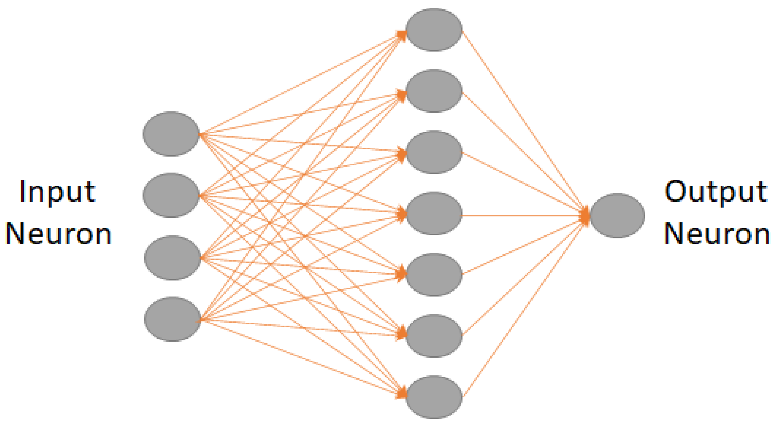
Using machine learning (ML) for gearbox predictive maintenance poses the key challenge of feature selection from extensive sensor data. The fully connected layer facilitates comprehensive connectivity between neurons across layers, enabling the learning of complex relationships between input features and output predictions [35]. Mathematically, it is represented as:

$$y=\sigma \left(W_{ij}X+b\right)$$

(12)

where $y$ is the output vector, W denotes the weight matrix defining connections between neurons, $X$ is the input vector, b is the bias vector, and σ signifies the activation function introducing non-linearity. It captures intricate data patterns essential for accurate predictions, making it a pivotal element in neural network design. Figure 12 depicts the layout of a fully-connected neural network layer. Table 1 shows the detailed parameters used for this study. For this study, nine networks, corresponding to nine distinct cases, were employed. These cases were categorized based on the total number of input layers, with options of 50, 100, and 500 units and normalization with z-score, none and z-center [36].

Figure 12. Layout of a fully connected neural network.

Table 1. Overview of the parameters of the fully connected later network.

Layer Type/Training Settings	Units
Feature layer	20 Features
FullyConnectedLayer1	(50, 100, 500) Fully connected layer
BatchNormalizationLayer	Batch normalization with 100 channels
RELULayer	ReLU
FullyConnectedLayer	2 fully connected layers
Softmaxlayer	Softmax
ClassificationOutputLayer	crossentropyex with classes “Faulty”/”Healthy”
Mini batchsize	10
Learning rate	0.001
Epochs	30

2.6. Performance Evaluation

Performance evaluation was crucial for assessing the effectiveness of the segmentation approaches, feature selection methods, and machine learning models employed in the study. The k-fold cross-validation (with k = 10) was used to compare the performances across different iterations. The dataset was divided into segments based on groups with windowing and bootstrapping methods, and the process was iterated 10 times. This was carried out with a view to ensuring that each group was used as the testing set. In each iteration, one group (70%) was reserved for testing, one (15%) for validation, and the remaining groups (15%) for training. The evaluation metrics of the testing results across all iterations were aggregated to determine the final system performance. Notably, the performance evaluation was conducted independently for two datasets. The system performance was analyzed using four evaluation metrics as below [37]:

$$Accuracy=\frac{TP+TN}{TP+FP+TN+FN}$$

(13)

$$Precision=\frac{TP}{TP+FP}$$

(14)

$$Sensitivity=\frac{TP}{TP+FN}$$

(15)

$$Specificity=\frac{TN}{FP+TN}$$

(16)

where

• TP (true positive): an occurrence is classified as TP if at least one predicted outcome is labelled “Healthy” when the true event value is labelled “Healthy”.
• FP (false positive): an occurrence is classified as FP if at least one outcome is labelled “Faulty” when the true event value is labelled “Healthy”.
• TN (true negative): an occurrence is classified as TN if at least one outcome is labelled “Faulty” when the true event value is labelled “Faulty”.
• FN (false negative): an occurrence is classified as TP if at least one outcome is labelled with “Healthy” when the true event value is labelled “Faulty”.

3. Results and Discussion

3.1. Experimental Scenarios Based on Feature Selection and Ranking

The experiment was carried out using different scenarios. The details of the experimental variables and the obtained accuracy are described below in the following section.

• SCENARIO 1: Gearbox Fault Diagnosis Using Raw Data without Feature Selection

For this case, the raw gearbox vibration dataset with classification as “Healthy” and “Faulty” was passed through different ML models. The model used in this case serves as a base model for experiment purposes. The dataset was distributed as 80% training and 20% testing with the 10-fold cross-validation method. Table 2 shows the accuracy results of the different machine learning algorithms. At first glance, the maximum accuracy that these models could achieve is 60.8% which is fairly low and other models performed quite poorly.

Table 2. Predictions based on raw data—without feature selection.

Prediction Model	Sub-Type	Accuracy in %
Decision tree	Fine tree	58.3
	Medium tree	57.8
	Coarse tree	55.3
Logistic regression 50.8		50.8
Naive Bayes (Gaussian)		56.6
KNN	Fine KNN	54.8
	Medium KNN	58.1
	Coarse KNN	60.8
	Cosine KNN	56.2
	Cubic KNN	58.0
	Weighted KNN	57.4

• SCENARIO 2: Gearbox Fault Diagnosis Using Raw Data with Feature Selection and without Ranking

The raw gearbox vibration dataset with classification as “Healthy” and “Faulty” with feature selection based on different condition indicators as described before was used. All available features were used in this case and no ranking was carried out. Additional models were employed to differentiate to provide further flexibility to the existing base models from the previous case. The dataset was distributed as 80% training and 20% testing with the 10-fold cross-validation method. Table 3 shows the accuracy results of the different ML algorithms. Here, it is seen that some models did outperform the previous case and the maximum accuracy was recorded as 93.8%, which reinstates the importance of using condition indicators to improve the overall performance of the predictive models. However, some new models that were added in this case did not perform well.

Table 3. Predictions based after feature selection without ranking.

Prediction Model	Sub-Type	Accuracy (%)
Decision tree	Fine tree	87.5
	Medium tree	87.5
	Coarse tree	87.5
Logistic regression		75
Naive Bayes	Gaussian	93.8
	Kernel	93.8
SVM	Linear	37.5
	Quadratic	37.5
	Cubic	37.5
	Fine Gaussian	37.5
	Medium Gaussian	37.5
	Coarse Gaussian	37.5
KNN	Fine KNN	37.5
	Medium KNN	37.5
	Coarse KNN	37.5
	Cosine KNN	37.5
	Cubic KNN	37.5
	Weighted KNN	37.5
Ensemble	Boosted trees	37.5
	Bagged trees	75
	Subspace discriminant	93.8
	Subspace KNN	75
	RUSBoosted trees	37.5
	Narrow neural network	37.5

• SCENARIO 3: Gearbox Fault Diagnosis Using Raw Data with Feature Selection and with Ranking

For this case, the raw gearbox vibration dataset with classification as “Healthy” and “Faulty” with feature selection based on different condition indicators as described previously was used. All available features were used in this case and a further process of ranking was performed. Here, the top 20 features were employed irrespective of channel consideration. For ranking, the one-way ANOVA method was utilized. The dataset was distributed as 80% training and 20% testing with 10-fold cross-validation method. Table 4 shows the accuracy results of the different ML algorithms, revealing that some models outperformed the previous case and the maximum accuracy was recorded to be 100% and the lowest was 37.5%. In this case, the models performed significantly better as compared to the previous scenario. These results show that the ranking can significantly alter the predictive capacity of the models.

Table 4. Predictions based after feature selection with ranking selection (one-ANOVA) based on top 20 features.

Prediction Model	Sub-Type	Accuracy (%)
Decision tree	Fine tree	87.5
	Medium tree	87.5
	Coarse tree	87.5
Logistic regression		87.5
Naive Bayes	Gaussian	100
	Kernel	93.8
SVM	Linear	43.8
	Quadratic	43.8
	Cubic	43.8
	Fine Gaussian	37.5
	Medium Gaussian	43.8
	Coarse Gaussian	43.8
KNN	Fine KNN	43.8
	Medium KNN	43.8
	Coarse KNN	37.5
	Cosine KNN	43.8
	Cubic KNN	43.8
	Weighted KNN	43.8
Ensemble	Boosted trees	37.5
	Bagged trees	87.5
	Subspace discriminant	100
	Subspace KNN	75
	RUSBoosted Trees	43.8
	Narrow neural network	43.8

• SCENARIO 4: Gearbox Fault Diagnosis Using Raw Data with Feature Selection and with Ranking

The raw gearbox vibration dataset with classification as “Healthy” and ”Faulty” with feature selection based on different condition indicators as described in the previous section was used. All the available features were used in this case and a further process of ranking was performed. Here, the top five features from each vibration channel were employed to have a consistent correlation from each channel to channel distribution. For ranking, the one-way ANOVA method was utilized. The dataset was distributed as 80% training and 20% testing with the 10-fold cross-validation method. Table 5 shows the accuracy results of the different machine learning algorithms. In this case, it is evident that some models did outperform the previous case and the maximum accuracy was recorded as 100% and other models did improve in terms of performance accuracy. In this case, the models performed significantly better as compared to the previous scenario, but the performance of two models (bagged trees and RUSBoosted trees) was seen to be declining. Bagged trees are employed to reduce variance within a noisy dataset and RUSboosted trees are used for improving classification performance when training data is imbalanced. As this case does not apply to the current database, the usage of this model can be excluded [38].

Table 5. Predictions based after feature selection with ranking selection (one-way ANOVA) based on top five features from the same channel.

Prediction Model	Sub-Type	Accuracy (%)
Decision tree	Fine tree	87.5
	Medium tree	87.5
	Coarse tree	87.5
Logistic regression		100
Naive Bayes	Gaussian	100
	Kernel	100
SVM	Linear	100
	Quadratic	100
	Cubic	100
	Fine Gaussian	62.5
	Medium Gaussian	100
	Coarse Gaussian	87.5
KNN	Fine KNN	100
	Medium KNN	75
	Coarse KNN	37.5
	Cosine KNN	93.8
	Cubic KNN	68.8
	Weighted KNN	100
Ensemble	Boosted trees	37.5
	Bagged trees	75
	Subspace discriminant	100
	Subspace KNN	100
	RUSBoosted trees	37.5
	Narrow neural network	93.8

3.2. Experimental Scenarios with Windowing and Bootstrapping

In order to address the challenge of managing larger datasets and mitigating the risk of overfitting in ML approaches, this study employed various deep learning models discussed in previous sections. These models are applied to a dataset that undergoes segmentation to enhance its capacity. The specifications for the fully connected layer parameters are outlined in Table 1. Detailed explanations of the data segmentation process and feature engineering methodologies utilized in this study are provided in the methodology section. The iterative process of bootstrapping and windowing leads to a significant advancement in the current research experiments, highlighting the critical role of data segmentation over conventional ML models.

• SCENARIO 1: Gearbox Fault Diagnosis Using windowing with Feature Selection and with Ranking (top five features for each channel)

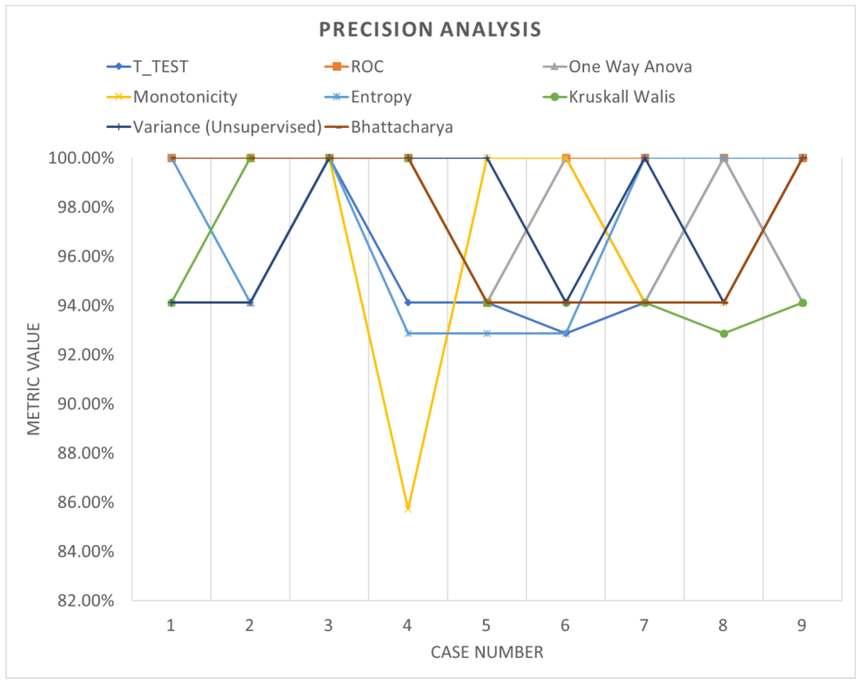
Table 6 shows the accuracy performance of the model under different parameter configurations when applied to segmented data using windowing. Upon detailed examination, it becomes apparent that employing various feature ranking methods enables the identification of the optimal accuracy for the system under evaluation. Windowing notably enhances accuracy performance, underscoring the increased adaptability and efficacy of these models. Figure 13, Figure 14 and Figure 15 offer a visual comparison of the performance evaluations. These visual representations elucidate the intricate relationships between metrics across different ranking schemes, highlighting the significance of factors such as the number of network layers and diverse normalization techniques, as elucidated in Table 7. The results indicate that configurations yielding optimal performance, as indicated by this metric, tend to converge towards case 3, characterized by normalization using z-score and a fully connected network comprising 500 layers.

Table 6. Accuracy distribution with a different ranking methods with windowing.

Ranking Method	Fully Connected Layer (RELU NETWORK)
	Normalization Z-Score			Normalization None			Normalization Z-Center
	Number of Layers
	50	100	500	50	100	500	50	100	500
T_TEST	96.97	96.97	96.97	93.94	93.94	90.91	93.94	87.88	93.94
ROC	100	100	100	100	93.94	96.97	96.97	96.97	100
One-way ANOVA	93.94	93.94	100	96.97	93.94	100	93.94	96.97	93.94
Monotonicity	96.97	96.97	96.97	75.76	96.97	96.97	93.94	93.94	81.82
Entropy	96.97	93.94	96.97	90.91	90.91	90.91	81.82	100	100
Kruskal–Wallis	93.94	96.97	96.97	96.97	93.94	93.94	93.94	90.91	93.94
Variance (unsupervised)	93.94	93.94	100	96.97	96.97	93.94	96.97	93.94	96.97
Bhattacharya	96.97	96.97	96.97	96.97	93.94	93.94	93.94	93.94	87.88

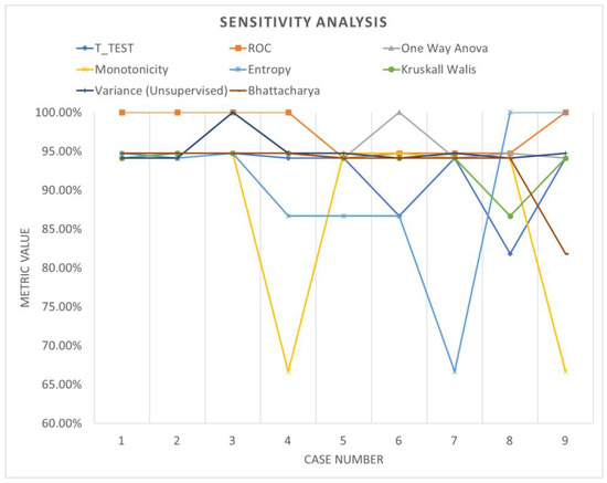
Figure 13. Sensitivity analysis (windowing).

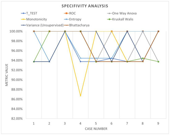
Figure 14. Specificity analysis (windowing).

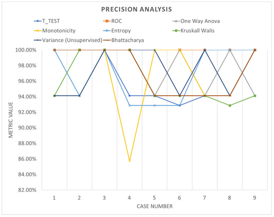
Figure 15. Precision analysis (windowing).

Table 7. Accuracy distribution with a different ranking method with bootstrapping.

Ranking Method	Fully Connected Layer (RELU NETWORK)
	Normalization Z-Score			Normalization None			Normalization Z-Center
	Number of Layers
	50	100	500	50	100	500	50	100	50
T_TEST	96.67	96.67	96.67	96.67	96.67	96.67	96.67	96.67	96.67
ROC	100	100	100	100	100	100	100	100	100
One-way ANOVA	93.33	93.33	93.33	93.33	93.33	93.33	93.33	93.33	93.33
Monotonicity	100	100	100	100	100	100	100	100	100
Entropy	96.67	96.67	96.67	96.67	96.67	96.67	96.67	96.67	96.67
Kruskal–Wallis	96.67	96.67	96.67	96.67	96.67	96.67	96.67	96.67	96.67
Variance (unsupervised)	93.33	93.33	93.33	93.33	93.33	93.33	93.33	93.33	93.33
Bhattacharya	96.67	96.67	100	100	96.67	96.67	96.67	96.67	96.67

• SCENARIO 2: Gearbox Fault Diagnosis Using bootstrapping with Feature Selection and with Ranking (top 5 feature for each channel)

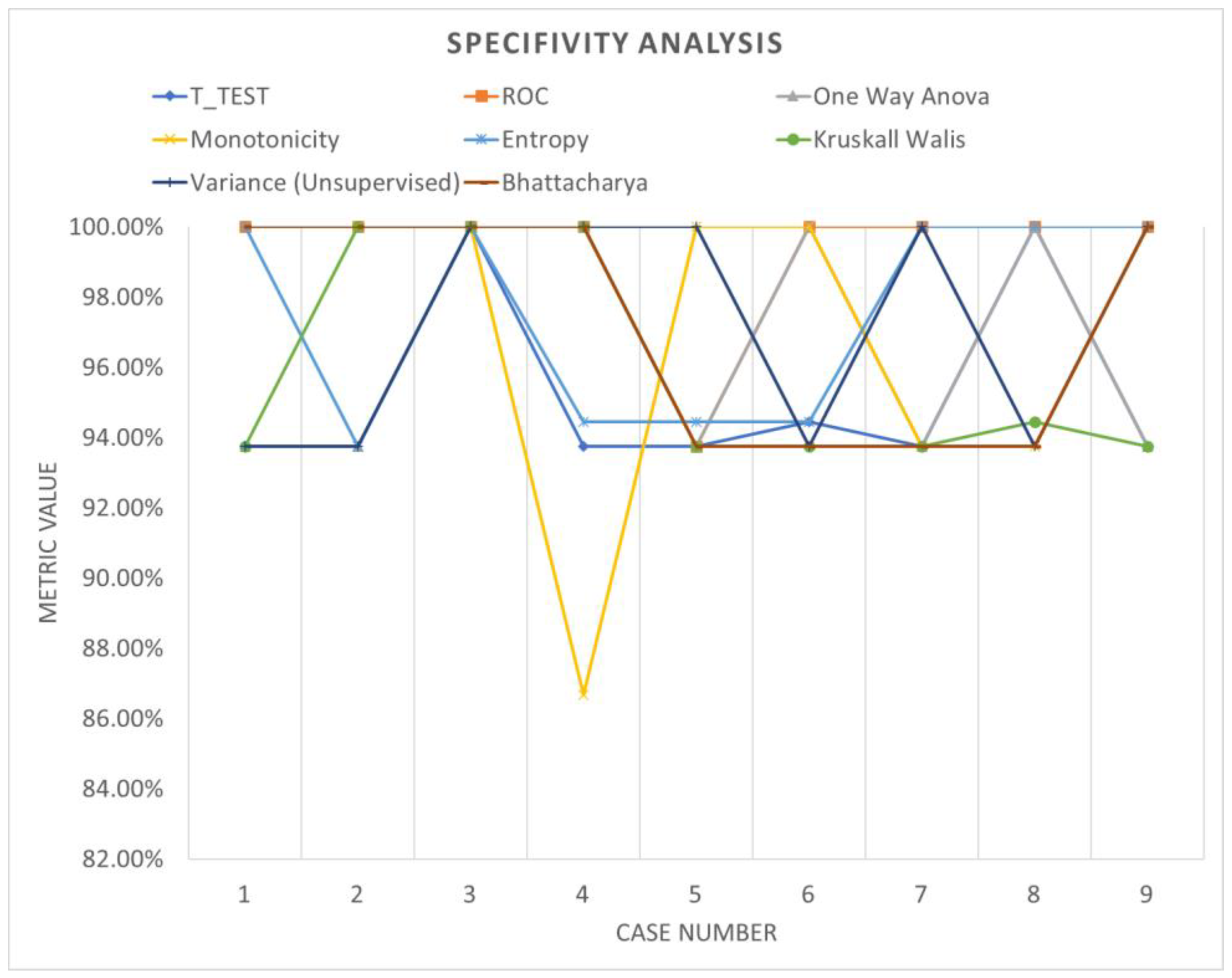
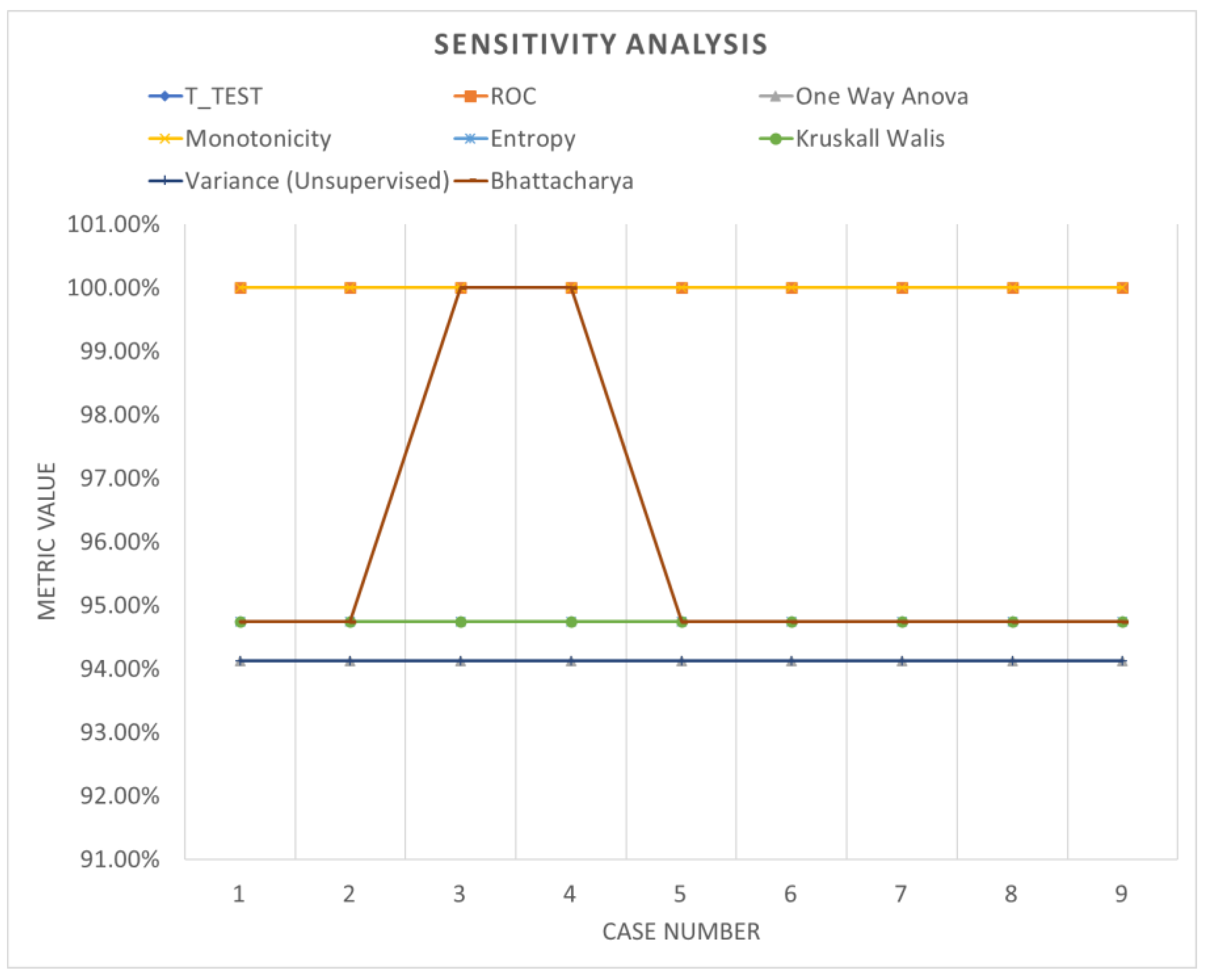
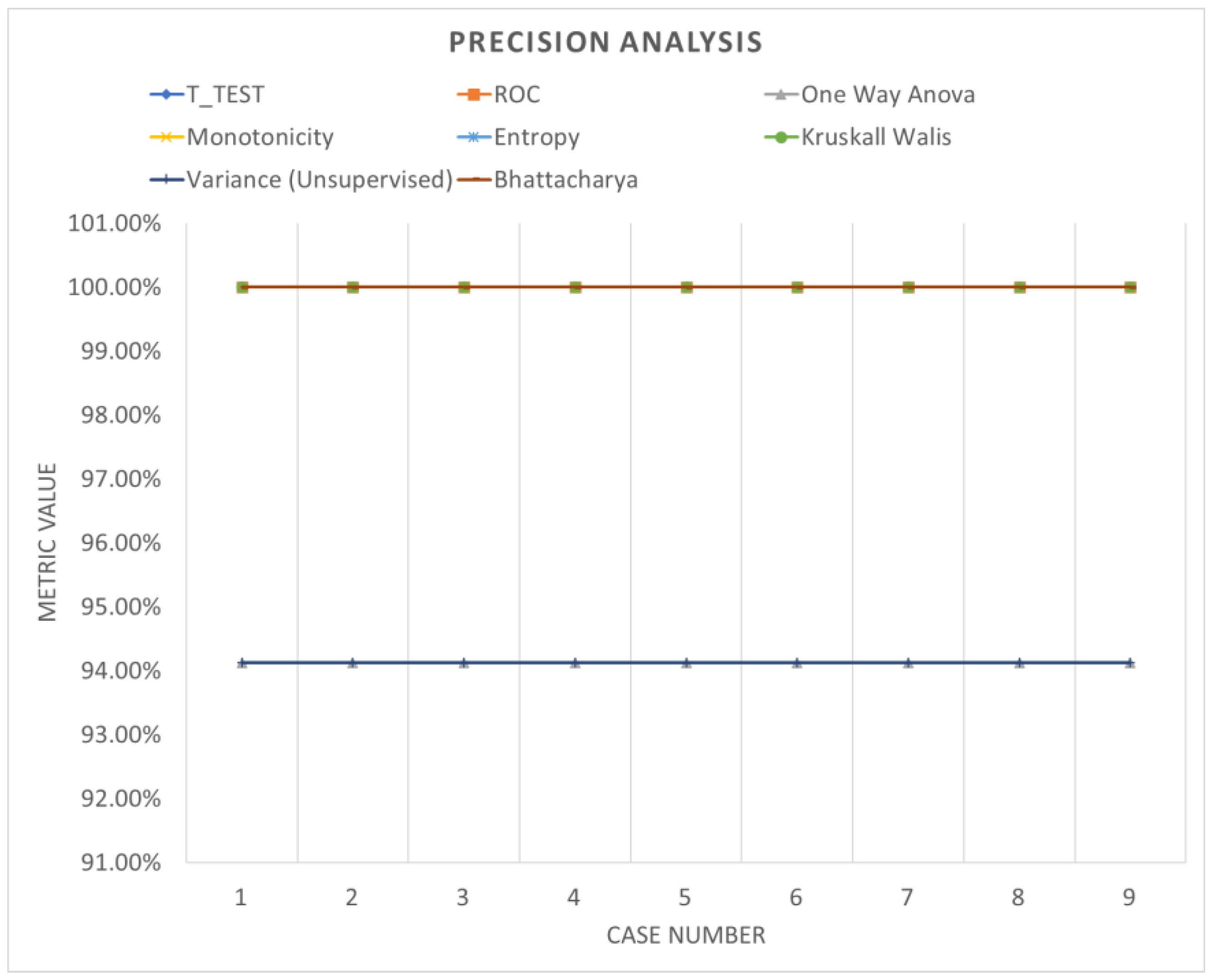
Table 7 shows the accuracy performance of the model which varies with different parameters when analyzed with data segmented using bootstrapping. Despite notable improvements in system performance, the accuracy remains relatively consistent and does not exhibit significant fluctuations with parameter adjustments. Figure 16, Figure 17 and Figure 18 offer a graphical representation of a comparative analysis involving various performance evaluations regarding the specificity, sensitivity and precision of the analysis. These visualizations highlight the fluctuations in metrics across different ranking schemes, underscoring the importance of both the number of network layers and the utilization of diverse normalization schemes, as outlined in Table 7. Minimal changes in performance evaluation were observed under these specific conditions, providing insights into the broader research narrative.

Figure 16. Sensitivity analysis (bootstrapping).

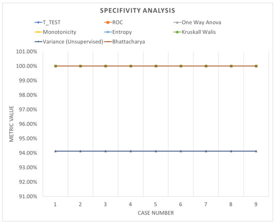
Figure 17. Specificity analysis (bootstrapping).

Figure 18. Precision analysis (bootstrapping).

3.3. Validation of the Results

To validate the efficacy of the proposed enhanced feature engineering, particularly focusing on the data segmentation process, another gearbox dataset was evaluated (referred to as HS—high-speed gearbox). This dataset comprised vibration data collected over a period of 6 s, sampled at a frequency of 97,656 Hz, from the three blades of an upwind V90 wind generator [39]. The data encompassed both normal operating conditions and fault conditions, with natural faults introduced in the pinion gear. Among the 17 files, 11 were identified as faulty, while 6 were deemed normal. Employing a fully connected network with parameters similar to those used in the first dataset, the accuracy distribution of the system utilizing all features without employing any ranking was analyzed, as depicted in Table 8. For further comparison, the same dataset was processed using windowing and bootstrapping techniques. Further, selective ranking methods were applied and their respective outputs were observed, as shown in Table 9 and Table 10, respectively. In these evaluations, the windowing method consistently exhibited substantial improvements, showcasing varied accuracy distributions influenced by different parameters and ranking techniques. This highlights its notable versatility and robustness in comparison to bootstrapping. Bootstrapping tended to lead to overfitting across most parameter changes, thereby demonstrating its limited efficacy as a preferable option.

Table 8. Validation test—accuracy distribution with all features and no ranking.

Ranking Method	Fully Connected Layer (RELU NETWORK)
	Normalization Z-Score			Normalization None			Normalization Z-Center
	Number of Layers
	50	100	500	50	100	500	50	100	50
All features	55	72.5	97.5	42.5	42.5	22.5	47.5	42.5	27.5

Table 9. Validation test—accuracy distribution with different ranking with windowing.

Ranking Method	Fully Connected Layer (RELU NETWORK)
	Normalization Z-Score			Normalization None			Normalization Z-Center
	Number of Layers
	50	100	500	50	100	500	50	100	50
TEST	96.25	100	100	83.75	87.5	93.75	84.38	86.88	94.38
Variance	99.38	99.38	100	66.88	72.5	95	60.63	75	93.13
Bhattacharya	100	100	100	98.75	97.5	96.25	96.88	96.88	96.25

Table 10. Validation test—Accuracy distribution with a different ranking with bootstrapping.

Ranking Method	Fully Connected Layer (RELU NETWORK)
	Normalization Z-Score			Normalization None			Normalization Z-Center
	Number of Layers
	50	100	500	50	100	500	50	100	50
TEST	100	100	100	100	100	97.78	100	100	97.04
Variance	100	100	100	100	100	97.78	100	100	97.04
Bhattacharya	100	100	100	94.07	98.52	98.15	95.56	100	97.04

4. Conclusions

The current study evaluated an enhanced feature engineering process incorporating various aspects of feature selection and data segmentation, in the context of gearbox predictive maintenance. Through a comparative analysis of different feature engineering and data segmentation methods, the study explored their impact on the performance and predictive capacity of the system. Various ML models, including neural networks, decision trees, support vector machines (SVM), k-nearest neighbor (kNN), naive Bayes, logistic regression models, and ensemble learning models, were subjected to different hyperparameters to assess their performance. The results indicate that careful consideration of feature selection and ranking methods can significantly improve overall accuracy, with decision trees (from 58.3% to 87.5%), SVM (from 37.5% to 100%), neural networks (from 37.5% to 93.8%) and KNN (from 37.5% to 100%) demonstrating particularly promising results compared to naive Bayes (from 93.8 to 100%), logistic regression models (from 75% to 100%) and ensemble learning models, as they seem to overfit with data variations. With ensemble learning, except for the subspace discrimination model and subspace KNN, the accuracy variation was minimal.

Moreover, within the framework of a fully connected network, different ranking methods were applied alongside data segmentation using windowing and bootstrapping techniques. The windowing technique exhibited greater flexibility, allowing for the exploration of various parameters and ranking methods, and was found to be more robust compared to bootstrapping, where the output remains constant regardless of parameters. The normalization z-score for 500 layers showed the highest accuracy when the windowing method was used. The ROC method was found to be the most accurate, and it had a 100% accuracy level for all three layers of 50, 100 and 500. Furthermore, the Kruskal–Wallis method, variance (unsupervised) and one-way ANOVA methods showed poor accuracy levels. With the validation, three ranking methods were used, which were the t-test, variance and the Bhattacharya method. With z-score normalization, all three methods gave an accuracy level of 100% for all three layers selected: 50, 100, and 500. Under the Bhattacharya method, for 50 layers, the accuracy level was minimal. It was 94.07% under the no normalization and 95.56% under the z-center. This observation was consistent across validation datasets. Consequently, the windowing technique is suggested as the preferable method due to its superior latency and performance efficiency. Nonetheless, further research is recommended to explore the potential of both windowing and bootstrapping techniques across datasets of varying complexity from different applications, thereby providing a comprehensive assessment of their overall performance.

References

- Durbhaka, G.K.; Selvaraj, B.; Mittal, M.; Saba, T.; Rehman, A.; Goyal, L.M. Swarmlstm: Condition monitoring of gearbox fault diagnosis based on hybrid lstm deep neural network optimized by swarm intelligence algorithms. Comput. Mater. Contin. 2020, 66, 2041–2059. [Google Scholar]
- Malik, H.; Pandya, Y.; Parashar, A.; Sharma, R. Feature extraction using emd and classifier through artificial neural networks for gearbox fault diagnosis. Adv. Intell. Syst. Comput. 2019, 697, 309–317. [Google Scholar]
- Gu, H.; Liu, W.; Gao, Q.; Zhang, Y. A review on wind turbines gearbox fault diagnosis methods. J. Vibroeng. 2021, 23, 26–43. [Google Scholar] [CrossRef]
- Shukla, K.; Nefti-Meziani, S.; Davis, S. A heuristic approach on predictive maintenance techniques: Limitations and Scope. Adv. Mech. Eng. 2022, 14, 16878132221101009. [Google Scholar] [CrossRef]
- Li, P.; Wang, Y.; Chen, J.; Zhang, J. Machinery fault diagnosis using deep one-class classification neural network. IEEE Trans. Ind. Electron. 2018, 66, 2420–2431. [Google Scholar]
- Li, P.; Wang, J.; Chen, J. Sensor feature selection for gearbox fault diagnosis based on improved mutual information. Measurement 2020, 150, 107018. [Google Scholar]
- Kernbach, J.M.; Staartjes, V.E. Foundations of machine learning-based clinical prediction modeling: Part ii—Generalization and overfitting. In Machine Learning in Clinical Neuroscience: Foundations and Applications; Springer: Cham, Switzerland, 2022; pp. 15–21. [Google Scholar]
- Gosiewska, A.; Kozak, A.; Biecek, P. Simpler is better: Lifting interpretability performance trade-off via automated feature engineering. Decis. Support Syst. 2021, 150, 113556. [Google Scholar] [CrossRef]
- Atex, J.M.; Smith, R.D. Data segmentation techniques for improved machine learning performance. J. Artif. Intell. Res. 2018, 25, 127–145. [Google Scholar]
- Atex, J.M.; Smith, R.D.; Johnson, L. Spatial segmentation in machine learning: Methods and applications. In Proceedings of the International Conference on Machine Learning, Long Beach, CA, USA, 9–15 June 2019; pp. 234–241. [Google Scholar]
- Silhavy, P.; Silhavy, R.; Prokopova, Z. Categorical variable segmentation model for software development effort estimation. IEEE Access 2019, 7, 9618–9626. [Google Scholar] [CrossRef]
- Giordano, D.; Giobergia, F.; Pastor, E.; La Macchia, A.; Cerquitelli, T.; Baralis, E.; Mellia, M.; Tricarico, D. Data-driven strategies for predictive maintenance: Lesson learned from an automotive use case. Comput. Ind. 2022, 134, 103554. [Google Scholar] [CrossRef]
- Bersch, S.D.; Azzi, D.; Khusainov, R.; Achumba, I.E.; Ries, J. Sensor data acquisition and processing parameters for human activity classification. Sensors 2014, 14, 4239–4270. [Google Scholar] [CrossRef] [PubMed]
- Putra, I.P.E.S.; Vesilo, R. Window-size impact on detection rate of wearablesensor-based fall detection using supervised machine learning. In Proceedings of the 2017 IEEE Life Sciences Conference (LSC), Sydney, Australia, 13–15 December 2017; pp. 21–26. [Google Scholar]
- Saraiva, S.V.; de Oliveira Carvalho, F.; Santos, C.A.G.; Barreto, L.C.; de Macedo Machado Freire, P.K. Daily streamflow forecasting in sobradinho reservoir using machine learning models coupled with wavelet transform and bootstrapping. Appl. Soft Comput. 2021, 102, 107081. [Google Scholar] [CrossRef]
- Sait, A.S.; Sharaf-Eldeen, Y.I. A review of gearbox condition monitoring based on vibration analysis techniques diagnostics and prognostics. Conf. Proc. Soc. Exp. Mech. Ser. 2011, 5, 307–324. [Google Scholar]
- Wang, D.; Zhang, H.; Liu, R.; Lv, W.; Wang, D. T-test feature selection approach based on term frequency for text categorization. Pattern Recognit. Lett. 2014, 45, 1–10. [Google Scholar] [CrossRef]
- Chen, X.W.; Wasikowski, M. Fast: A roc-based feature selection metric for small samples and imbalanced data classification problems. In Proceedings of the 14th ACM SIGKDD International Conference on Knowledge Discovery and Data Mining, Las Vegas, NV, USA, 24–27 August 2008; pp. 124–132. [Google Scholar]
- Pawlik, P.; Kania, K.; Przysucha, B. The use of deep learning methods in diagnosing rotating machines operating in variable conditions. Energies 2021, 14, 4231. [Google Scholar] [CrossRef]
- Ompusunggu, A.P. On improving the monotonicity-based evaluation method for selecting features/health indicators for prognostics. In Proceedings of the 2020 11th International Conference on Prognostics and System Health Management (PHM-2020 Jinan), Jinan, China, 23–25 October 2020; pp. 242–246. [Google Scholar]
- Ramteke, D.S.; Parey, A.; Pachori, R.B. Automated gear fault detection of micron level wear in bevel gears using variational mode decomposition. J. Mech. Sci. Technol. 2019, 33, 5769–5777. [Google Scholar] [CrossRef]
- Ebenuwa, S.H.; Sharif, M.S.; Alazab, M.; Al-Nemrat, A. Variance ranking attributes selection techniques for binary classification problem in imbalance data. IEEE Access 2019, 7, 24649–24666. [Google Scholar] [CrossRef]
- Momenzadeh, M.; Sehhati, M.; Rabbani, H. A novel feature selection method for microarray data classification based on hidden markov model. J. Biomed. Inform. 2019, 95, 103213. [Google Scholar] [CrossRef] [PubMed]
- Ratner, B. The correlation coefficient: Its values range between 1/1, or do they. J. Target. Meas. Anal. Mark. 2009, 17, 139–142. [Google Scholar] [CrossRef]
- Mukaka, M.M. A guide to appropriate use of correlation coefficient in medical research. Malawi Med. J. 2012, 24, 69. [Google Scholar]
- Mohsin, M.F.M.; Hamdan, A.R.; Bakar, A.A. The effect of normalization for real value negative selection algorithm. In Soft Computing Applications and Intelligent Systems; Noah, S.A., Abdullah, A., Arshad, H., Bakar, A.A., Othman, Z.A., Sahran, S., Omar, N., Othman, Z., Eds.; Springer: Berlin/Heidelberg, Germany, 2013; pp. 194–205. [Google Scholar]
- Dangut, M.D.; Skaf, Z.; Jennions, I.K. An integrated machine learning model for aircraft components rare failure prognostics with log-based dataset. ISA Trans. 2021, 113, 127–139. [Google Scholar] [CrossRef] [PubMed]
- Lin, S.-L. Application of machine learning to a medium gaussian support vector machine in the diagnosis of motor bearing faults. Electronics 2021, 10, 2266. [Google Scholar] [CrossRef]
- Sun, L.; Liu, T.; Xie, Y.; Zhang, D.; Xia, X. Real-time power prediction approach for turbine using deep learning techniques. Energy 2021, 233, 121130. [Google Scholar] [CrossRef]
- Keartland, S.; Van Zyl, T.L. Automating predictive maintenance using oil analysis and machine learning. In Proceedings of the 2020 International AUPEC/RobMech/PRASA Conference, Cape Town, South Africa, 29–31 January 2020; pp. 1–6. [Google Scholar]
- van Dinter, R.; Tekinerdogan, B.; Catal, C. Predictive maintenance using digital twins: A systematic literature review. Inf. Softw. Technol. 2022, 151, 107008. [Google Scholar] [CrossRef]
- Wang, Z.; Huang, H.; Wang, Y. Fault diagnosis of planetary gearbox using multi-criteria feature selection and heterogeneous ensemble learning classification. Measurement 2021, 173, 108654. [Google Scholar] [CrossRef]
- Chandrasekaran, M.; Sonawane, P.R.; Sriramya, P. Prediction of gear pitting severity by using naive bayes machine learning algorithm. In Recent Advances in Materials and Modern Manufacturing; Springer: Singapore, 2022; pp. 131–141. [Google Scholar]
- Xu, Y.; Nascimento, N.M.M.; de Sousa, P.H.F.; Nogueira, F.G.; Torrico, B.C.; Han, T.; Jia, C.; Filho, P.P.R. Multi-sensor edge computing architecture for identification of failures short-circuits in wind turbine generators. Appl. Soft Comput. 2021, 101, 107053. [Google Scholar] [CrossRef]
- Goodfellow, I.; Bengio, Y.; Courville, A. Deep Learning; MIT Press: Cambridge, MA, USA, 2016. [Google Scholar]
- Hu, H. Feature convolutional networks. In Proceedings of the 13th Asian Conference on Machine Learning, Virtual, 19 November 2021; Volume 157, pp. 830–839. [Google Scholar]
- Hesabi, H.; Nourelfath, M.; Hajji, A. A deep learning predictive model for selective maintenance optimization. Reliab. Eng. Syst. Saf. 2022, 219, 108191. [Google Scholar] [CrossRef]
- KGP, K.I. Bagging and Random Forests: Reducing Bias and Variance Using Randomness by kdag iit kgp Medium. Available online: https://kdagiit.medium.com/ (accessed on 5 March 2024).
- Bechhoefer, E. High Speed Gear Dataset. Available online: https://www.kau-sdol.com/kaug (accessed on 6 December 2012).
Disclaimer/Publisher’s Note: The statements, opinions and data contained in all publications are solely those of the individual author(s) and contributor(s) and not of MDPI and/or the editor(s). MDPI and/or the editor(s) disclaim responsibility for any injury to people or property resulting from any ideas, methods, instructions or products referred to in the content. |
© 2024 by the authors. Licensee MDPI, Basel, Switzerland. This article is an open access article distributed under the terms and conditions of the Creative Commons Attribution (CC BY) license (https://creativecommons.org/licenses/by/4.0/).