Finite Element Analysis of Different Transverse Flux Linear Induction Motor Models to Improve the Performance of the Main Magnetic Circuit

Abstract

This paper delves into the knowledge of transverse flux linear induction motors using three-dimensional finite element simulation tools. Original linear induction motors have a useful magnetic flux perpendicular to the movement. We propose some geometric changes to improve the main magnetic circuit of the machine and to ensure simultaneous operation between longitudinal and transverse magnetic fluxes. To obtain the main parameters of the equivalent electrical circuit in a steady state, we propose two steps. Firstly, replicate the classic indirect tests used in rotating machines. This represents a significant advantage since it allows several models to be experimentally tested to obtain the values of electrical parameters. Secondly, use the data from these tests to solve a particular system of equations using numerical methods. The solution provides the electrical elements necessary to generate the equivalent circuit proposed by the authors. A quantitative analysis of the main electrical parameters is also carried out, confirming the advantages of the changes introduced. With them, a significant improvement in thrust force is obtained, especially in stationary conditions and low speeds. Finally, we study, in detail, a set of specific phenomena of linear machines using two parameters: the secondary equivalent air gap and the secondary equivalent conductivity.

1. Introduction

A linear induction motor (LIM) is a machine that can develop a thrust force along the direction of the movement. The applications of LIMs are increasing in both civilian and military sectors. In passenger transport, Maglev trains stand out [1], while in the automotive and aerospace industries, the production of components using magnetohydrodynamic technologies allows the creation of more reliable parts capable of withstanding several mechanical stresses and loads. Electromagnetic catapults are already used on the decks of aircraft carriers to launch aircraft, and electromagnetic cannons could be a revolutionary weapon for the future of artillery [2,3,4,5]. Consequently, there is a growing need for more sophisticated and faster control devices that allow optimum control of this type of motor. Any control technique requires, as a starting point, an adequate knowledge of the plant or system to be controlled. However, even considering the advances in speed regulation in electric machines, linear electric devices present a set of specific characteristics that make the electrical parameters difficult to understand.

The research carried out in this work represents a relevant contribution to the advancement of knowledge in linear induction motors, especially those with transverse magnetic flux configuration. The analysis of useful magnetic fluxes in motors reveals that by introducing some specific changes to the original magnetic circuit, it is possible to achieve a final mixed magnetic flux configuration. So, in our paper, we propose a methodology to determine an electric equivalent circuit (EC) corresponding to a mixed flux linear induction motor (MFLIM). To this end, we developed three different models to improve the original configuration of a transverse flux linear induction motor (TFLIM). We include different geometric changes to obtain an LIM where longitudinal and transverse magnetic fluxes can simultaneously operate [6,7,8,9]. Primarily, they are necessary for two relevant changes in the initial geometry. The first modification aims to reduce the transverse edge effect and to facilitate both the lateral and central teeth of the TFLIM to contribute to the generation of a thrust force in the direction of movement. The second change aims to allow the movement of a new useful magnetic flux along the longitudinal direction, which operates simultaneously with the initial transverse magnetic flux. One of the main novelties presented in the paper compared to [8,9] is that the different TFLIM models are simulated to obtain a comprehensive analysis of the characteristic curves (thrust force and vertical force). From this analysis, we can conclude that the proposed geometric changes improve the performance of the main magnetic circuit of the TFLIM. In addition, these changes imply a considerable improvement in the performance of the LIM without the need to increase the electrical power supply.

Specifically, these models are built in five stages using two different tools, FEM-3D and Matlab. With 3-D finite elements (FEM-3D) we have simulated the LIMs where we carried out the classic indirect tests used in rotating induction motors (RIMs). FEM-3D tools are very useful in the design of electric machines [10,11,12]. Reference [10] includes widely used FEM simulations of rotating electromagnetic devices with transverse flow, such as the Fractional Slot Concentrated Winding—Permanent Magnet Brushless DC (FSCW PMBLDC). In these devices, geometric changes are made to increase the useful magnetic flux and to improve the initial design. In an RIM, the use of 2-D simulations is enough to determine the main forces present in the motor, to analyse magnetic inductions in the air gap, or to calculate the inductance matrix. However, we need a more comprehensive study of the proposed TFLIM topologies, which implies the need to use 3-D tools and dynamic simulations where the moving part has a predetermined speed. All of this requires a significant computational effort to ensure that the solution converges successfully.

The EC proposed in this paper is based on the T-Type equivalent circuit commented in [13,14]. In [15], EC based on a Quasi-Two-Dimensional vertical analytical model for the case of a double-sided LIM, both in dynamic and steady state, was developed. This model will be modified to include the intrinsic characteristics of the open-air gap structure presented in the LIMs. To this end, we follow two different theories [16,17], modify the parallel branch of the EC, and adapt the modelling of RIMs to LIMs. In this paper, we focus only on obtaining the parameters corresponding to the steady state. Using Matlab, we designed and executed a method to obtain the main electric parameters of the EC for the three different models proposed in the paper.

This paper is organized as follows. Section 2 describes the main physics and geometrical properties of each TFLIM model. The main differences between topologies and the magnetic characteristics used in the simulations are detailed. In Section 3, we present the five stages used to calculate the main electric parameters of the EC. In Section 4, the main forces developed by each TFLIM model will be determined. In Section 5, the locked rotor and no-load secondary tests traditionally used in RIM are simulated using FEM-3D. Section 6 describes the equations that we propose to determine the parameters of the EC. In Section 7, we present a detailed analysis of the secondary equivalent air gap and secondary equivalent conductivity. Finally, the main results and conclusions are shown in Section 8.

2. TFLIM Proposed Models

In this section, we describe the three TFLIM topologies analyzed in our paper. First, we detail the main dimension and physical properties associated with our initial model called Model 1. Secondly, we present models 2 and 3, where we introduce changes in the geometry in both the primary and secondary parts. Finally, we check the advantages of the proposed changes by analyzing the characteristic curve, thrust force versus slip.

Model 1, described in [17] and represented in Figure 1, simulates a transverse magnetic flux configuration where the primary part is composed of 31 magnetic sheets with an E-shape design, whose design and dimensions are represented in the upper right part of Figure 1. The secondary part is composed of two layers where the first layer is made of aluminium and the second layer is a ferromagnetic plate, which is shown in the lower part of Figure 1. The primary part has a total length of 503.5 mm, a height of 115 mm, and a fixed width of 172 mm. The dimensions of the secondary part vary depending on the layer. Thus, the first aluminium layer has a length, width, and thickness of 990 mm, 300 mm, and 10 mm, respectively. And in the upper ferromagnetic backing, length, width, and thickness are 970 mm, 195 mm, and 25 mm, respectively.

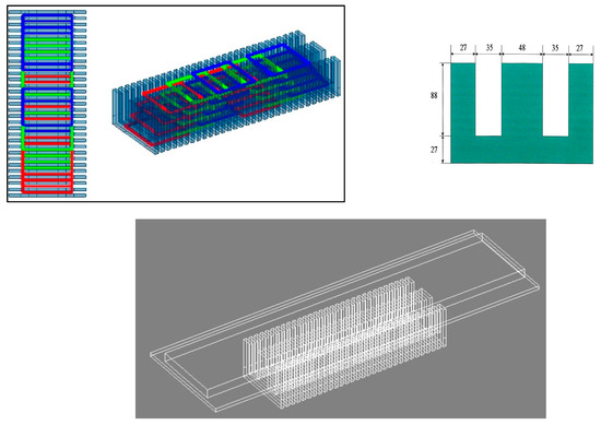
Figure 1. Primary part design, distribution of coils inside the TFLIM armature, and 3D view of Model 1.

Inside the primary part, the alternating current (AC) winding that generates a traveling magnetic wave, defined by the synchronous velocity $v_{sync} (\mathrm{m}/\mathrm{s})=20$ [8,18], is located. The upper left of Figure 1 shows the primary part design, where we can see three different phases. Phase A is represented with red coils, phase B with blue coils, and phase C with green coils [8]. AC winding presents three main properties: the number of slots per pole and phase (q) whose value is 4; the pole pitch ${\tau }_p=200 \mathrm{m}\mathrm{m}$, and the number of turns per phase $N_{turns}=44$. Additionally, the value of the winding factor $K_{W1}=0.6773$ is provided, which is thoroughly explained in [9]. Furthermore, it is important to remark that we set our voltage source level as a function of the magnetic field density across the air gap, $B_{gap} \left[T\right]$ [19]. We limited the value of $B_{gap}=0.8 \mathrm{T},$ and so, the line voltage level is fixed to $V_{LINE}=660 \mathrm{V}.$

Table 1 shows the main geometric dimensions of the TFLIM related to Figure 1. The values of the main electrical and magnetic magnitudes of the materials (aluminium, steel, and copper) used in the simulations are also specified in this table. The two most relevant properties to the simulations are electrical conductivity and magnetic permeability, as can be observed in Table 1. During the simulation, the evolution of temperature in the resistivity values of the materials used was not considered. The established operating temperature for the simulations was set to 25 °C. A detailed analysis to obtain these values is described in [8,9].

Table 1. Dimensions and main properties of TFLIM models [17].

TFLIM Geometric Parameters (mm)
Primary Part Dimension		Secondary Part Dimension
Width Longitudinal Slot	8.5	Aluminium Layer		Steel Layer
Slot Pitch	16.5	Thickness Aluminium	10	Thickness Steel	25
Primary Part Length	503.5	Width Aluminium	300	Width Steel	195
Pole pitch	200	Length Aluminium	990	Length Steel	970
Mechanical Air gap					5
Material Properties used in FEM 3-D
Electrical/magnetic quantities		Aluminium	Steel	Cooper
Conductivity/Resistivity		3.73·107 S/m	0 S/m	2.37·10−2 Ω∙mm2/m
Relative Permeability		1	2500	1
Properties of Primary Winding
${\mathit{\tau }}_{\mathit{p}}$		$\mathit{q}$	${\mathit{K}}_{\mathit{w}1}$	${\mathit{N}}_{\mathit{t}\mathit{u}\mathit{r}\mathit{n}\mathit{s}}$
200 mm		4	0.6773	44

In the paper, the iron losses were neglected due to the chosen electrical and magnetic properties. The zero electric conductivity of the steel implies the absence of eddy currents in the ferromagnetic parts (second layer in the moving part and primary part), and the linear B-H curve determines that there are no regions inside the LIM working under magnetic saturation conditions. If we consider the electrical conductivity in the steel layer implies the need to model the non-linear B-H curve of the ferromagnetic material because the TFLIM operates under magnetic saturation conditions. To this end, we should consider the following: (1) the circulation of induced electric currents inside the steel sheet is established, ${\overrightarrow{j}}_{eddy\_currents} (\raisebox{1ex}{$\mathrm{A}$}\!\left/ \!\raisebox{-1ex}{${\mathrm{m}\mathrm{m}}^2$}\right.)$; (2) according to Ampere’s Law, the magnetic field intensity ${\overrightarrow{H}}_{steel\_layer} (\raisebox{1ex}{$\mathrm{A}$}\!\left/ \!\raisebox{-1ex}{$\mathrm{m}$}\right.)$ is established; and (3) the magnetic field density vector inside the steel layer is generated, ${\overrightarrow{B}}_{steel\_layer} (\mathrm{T})$. This set of iterations in a material with nonlinear properties implies a high computational effort. This magnetic behaviour of the motor’s secondary of the TFLIM is explained in detail in [8]. One of the most important consequences of considering that the electric conductivity is equal to zero in the second layer of the secondary part is that the iron losses are neglected according to Equation (1), where $P_{Fe}$ is the power loss in the iron core; $P_{eddy}$ is the power eddy current loss; $P_h$ is the power hysteresis loss, all measured in W [8,20,21].

$$P_{Fe}=\underset{{\sigma }_{Fe}=0 \mathrm{S}/\mathrm{m}}{\underbrace{P_{eddy}}}+\underset{{\mu }_r=2500}{\underbrace{P_h}}=0 \mathrm{W}$$

(1)

Using Model 1 as a starting point, we simulate another two models, making geometric modifications to them. All proposed changes improve the net thrust force, thus optimizing the initial magnetic design. The new models are called Model 2 and Model 3, whose changes are discussed below:

In Model 2, we include two non-conducting slots into the aluminium layer. Both slots shown in the upper part of Figure 2 have a width of 1 mm. That implies the generation of three different regions inside the aluminium layer, where the eddy currents generate a positive thrust force along the movement $\left(F_y\right)$. $F_y$ is the sum of the thrust force generated in the aluminium layer $\left(F_{y\_Al}\right)$ and the thrust force of the top layer of ferromagnetic material $\left(F_{y\_Fe}\right)$ (see Equation (2)). In this paper, we want to minimize the computational effort during the 3D simulations, so the electrical conductivity of iron is considered equal to zero $\left({\sigma }_{Fe}=0 \mathrm{S}/\mathrm{m}\right)$. Consequently, the thrust force generated in this layer does not exist, $F_{y\_Fe}=0 \mathrm{N}$. Under these conditions, three independent loops of induced electric currents are generated in the aluminium layer of the secondary part. Each loop occurs above the central tooth and the side teeth of the primary part, generating a force above each tooth in the direction of movement (for more details, see [8]). Equation (3) shows that the only useful magnetic flux $\left({\varnothing }_{useful}\right)$ is the transverse flux ${(\varnothing }_{transversal})$, whose main path is formed by two segments. The central teeth of the primary one form this first segment. This flux, when the magnetic flux reaches the head of the central teeth (${\varnothing }_{centra{l}_{teeth}}$), is divided into two identical lateral magnetic fluxes ${(\varnothing }_{righ{t}_{teeth}}{,\varnothing }_{lef{t}_{teeth}})$ that circulate through the two lateral teeth that constitute the second segment of the main magnetic circuit.

$$F_y=F_{y\_Al}+\underset{{\sigma }_{Fe}=0 S/m}{\underbrace{F_{y\_Fe}}}=\underset{>0}{\underbrace{F_{y_{central\_teeth}}}}+\underset{>0}{\underbrace{F_{y_{transversal\_teeth}}}}$$

(2)

$${\mathrm{\varnothing }}_{useful}\approx {\mathrm{\varnothing }}_{transversal}⟶{\mathrm{\varnothing }}_{righ{t}_{teeth}}\approx {\mathrm{\varnothing }}_{lef{t}_{teeth}}\approx \raisebox{1ex}{${\mathrm{\varnothing }}_{centra{l}_{teeth}}$}\!\left/ \!\raisebox{-1ex}{$2$}\right.$$

(3)

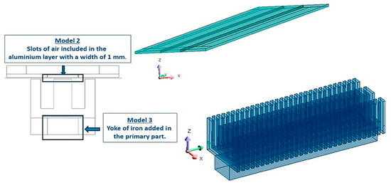
Figure 2. Geometrical changes in the Model 1 TFLIM to obtain Model 2 and Model 3.

In Model 3, we add a longitudinal magnetic flux, including a ferromagnetic yoke under the central teeth, as can be seen in the lower part of Figure 2. It is important to note that Model 1 and Model 2 operate with a transverse magnetic flux. The height of the new ferromagnetic structure is 50 mm, and the width is 83 mm. The structure extends along the entire length of the primary part, which is equivalent to a length of 503.5 mm. Model 3 represents an LIM operating with a mixed magnetic flux configuration, where transverse and longitudinal fluxes operate simultaneously. Equation (4) describes that the useful magnetic flux that circulates through the main magnetic circuit of the TFLIM is the combined effect of the transverse flux and a new longitudinal flux ${(\varnothing }_{longitudinal})$. Figure 2 shows the changes made in Model 1 to obtain Model 2 and Model 3.

$${\mathrm{\varnothing }}_{useful}\approx {\mathrm{\varnothing }}_{transversal}+{\mathrm{\varnothing }}_{longitudinal}$$

(4)

3. Methodology to Determine the EC Parameters

In this section, we present the methodology that we propose to determine the EC parameter. Our methodology is composed of five stages and uses two different tools. All stages of the methodology are described below. See Figure 3 for more details.

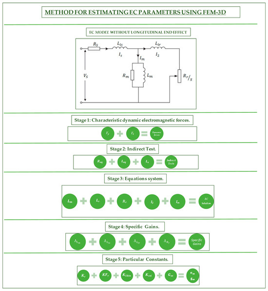
Figure 3. Methodology to determine the EC parameters.

• Stage 1. Characteristic dynamic electromagnetic forces. In this stage, we check the improvement in the thrust force developed by the proposed models once we have introduced the selected changes into the geometry. With the FEM-3D tool, we build the characteristic curve ‘Forces versus slip’ to justify the need to incorporate changes in our original TFLIM. The objective is that the analysed TFLIM topologies generate a thrust force greater than the force generated by our initial model without adding any increase in the voltage sources. Therefore, we represent the evolution of thrust forces $F_y$ and vertical forces $F_z$ throughout the entire sliding range. The transversal forces $F_x$ are neglected in this paper due to the low relevance of these forces [17,19].
• Stage 2. Indirect Test. In this stage, the typical indirect tests carried out in electrical machine laboratories to identify the EC parameters are simulated with the FEM-3D tool. The indirect test can be classified into two types: test under standstill conditions and test under no-load conditions. We simulate both. Firstly, we simulate TFLIM models under blocked secondary conditions (standstill conditions), and secondly, we simulate our electrical devices under no-load conditions. The range of frequencies is selected to obtain the most representative results. Both tests give us the values of three parameters: $R_{eq}$, $L_{eq}$, and $L_s$. These parameters will be studied in detail in Section 5.
• Stage 3. System of Equations: After we simulated the indirect tests, we proposed a system of equations to determine the main EC parameters per phase. This system of equations is computed with Matlab and we consider the obtained results from the previous stages to implement it. LEE is not included, so we only analyse the following five parameters: magnetizing inductance $L_m$, total secondary inductance $L_r$, secondary resistance $R_r$, secondary electric current $I_2$, and magnetizing electric current $I_m$, [18]. Using the obtained data from stages 1 to 3, we can determine the EC parameters by an accurate method. With the 3-D simulations, we considered a particular phenomenon (transversal and longitudinal magnetic fluxes operate simultaneously) of this type of LIM. This is not possible if we use a 2-D simulation. The five electrical parameters mentioned above are represented at the top of Figure 3. These parameters will be defined and discussed in Section 6. It is important to note in the graphical representation of the EC the absence of an additional parallel branch that considers the LEE by calculating two important dimensionless constants, $K_{Lm}$ and $K_{Rr}$, [16,17].
• Stage 4. Specific Gains: To compare the results obtained in the different models, we need four new KPIs to evaluate the changes in the EC parameters using the three TFLIM models proposed. To this end, it is necessary to establish an intermediate group of ratios to estimate the sensitivity of each parameter of the equivalent circuit when geometric changes are introduced. These new dimensionless indicators are ${\Lambda }_{{\mathrm{L}}_{\mathrm{m}}}$,${\Lambda }_{{\mathrm{L}}_{\mathrm{l}\mathrm{s}}}$, ${\Lambda }_{{\mathrm{L}}_{\mathrm{l}\mathrm{r}}}$, and ${\Lambda }_{\mathrm{R}\mathrm{r}}$. These indicators will be described in more detail in Section 6. They represent the magnitude of variations in the main parameters of the EC in percentage terms. These changes may imply a significant modification in the thrust force. These parameters are defined in this paper because it is necessary to establish a new gain to response to the introduced geometric changes, and they are not defined in the literature. Authors designed them to facilitate the control of a TFLIM in a future work.
• Stage 5. Particular constant: To complete the study of our TFLIM topologies, it is necessary to extend our analysis to include some particular phenomena that occur in LIM. So, we will study the Carter´s coefficient ($K_c$), fringing effect ($K_{Fr}$), skin effect ($K_{Skin}$), and goodness factor ($G_{se}$) to estimate two new indicators that allow us to evaluate these phenomena: equivalent electric conductivity $\left({\sigma }_{se}\right)$ and equivalent air gap $\left(g_{se}\right)$.

4. Characteristic Dynamic Electromagnetic Forces

In this section, we present the obtained results when we simulate with FEM 3-D the three TFLIM models under dynamic conditions [8]. Precisely, these thrust force values were calculated using the following scheme. Firstly, to carry out the simulations in FEM-3D, they were executed in a transient regime. Secondly, once the simulation reaches a steady state, we obtain the values of the forces, including both thrust and vertical forces, whether attractive or levitation.

This analysis shows the advantages of adding the proposed geometric changes in Model 2 and Model 3. We analyse the evolution of two main forces, thrust force (${\overrightarrow{F}}_y$) and levitation force (${\overrightarrow{F}}_z$). We will proceed to identify areas of optimum performance and areas where these forces do not present all the desired advantages. The behaviour of these forces during the beginning of the simulation is very important. We focused our analysis when the slip (s) varied from 1 to 0 (Table 2 shows the associated velocity to each value of the slip).

Table 2. Range of slips and velocities simulated with FEM-3D.

Dynamic Conditions for the Motion Analysis
Slip	0	0.1	0.2	0.3	0.4	0.5	0.6	0.7	0.8	0.9	1
Velocity (m/s)	20	18	16	14	12	10	8	6	4	2	0

The behaviour of ${\overrightarrow{F}}_y$ is shown in Figure 4. There, we have three main regions:

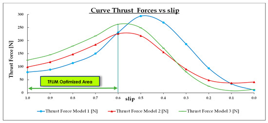
Figure 4. Characteristic curve thrust force versus slip.

• Region I (Low Velocities Zone): 0.6 < s < 1 ↔ $0 \raisebox{1ex}{$\mathrm{m}$}\!\left/ \!\raisebox{-1ex}{$\mathrm{s}$}\right.<{\overrightarrow{\mathrm{v}}}_{\mathrm{m}\mathrm{o}\mathrm{v}\mathrm{i}\mathrm{n}\mathrm{g}\_\mathrm{p}\mathrm{a}\mathrm{r}\mathrm{t}}<8 \raisebox{1ex}{$\mathrm{m}$}\!\left/ \!\raisebox{-1ex}{$\mathrm{s}$}\right.$;
• Region II (Medium Velocities Zone): 0.3 < s < 0.6 ↔ $8 \raisebox{1ex}{$\mathrm{m}$}\!\left/ \!\raisebox{-1ex}{$\mathrm{s}$}\right.<{\overrightarrow{\mathrm{v}}}_{\mathrm{m}\mathrm{o}\mathrm{v}\mathrm{i}\mathrm{n}\mathrm{g}\_\mathrm{p}\mathrm{a}\mathrm{r}\mathrm{t}}<14 \raisebox{1ex}{$\mathrm{m}$}\!\left/ \!\raisebox{-1ex}{$\mathrm{s}$}\right.$;
• Region III (High Velocities Zone): 0 < s < 0.3 ↔ $14 \raisebox{1ex}{$\mathrm{m}$}\!\left/ \!\raisebox{-1ex}{$\mathrm{s}$}\right.<{\overrightarrow{\mathrm{v}}}_{\mathrm{m}\mathrm{o}\mathrm{v}\mathrm{i}\mathrm{n}\mathrm{g}\_\mathrm{p}\mathrm{a}\mathrm{r}\mathrm{t}}<20 \raisebox{1ex}{$\mathrm{m}$}\!\left/ \!\raisebox{-1ex}{$\mathrm{s}$}\right.$.

In Region I, ${\overrightarrow{F}}_{y\_Model\_3}>{\overrightarrow{F}}_{y\_Model\_2}>{\overrightarrow{F}}_{y\_Model\_1}$. This situation is like a motor that operates under standstill conditions (slip equal to one), and we can see an improvement in the thrust force developed by Models 2 and 3. This is because a mixed magnetic flux configuration implies an increment in the thrust force with respect to our initial transverse magnetic flux topology. This difference in thrust force between Model 1 and 3 can be estimated around ${\left(∆{\overrightarrow{F}}_{3-1}\right)}_{RegionI}\approx 45.59 \mathrm{N}.$ that supposes a high rise close to 58%.

When the TFLIM operates at medium velocities (Region II), the behaviour changes ${\overrightarrow{F}}_{y\_Model\_1}>{\overrightarrow{F}}_{y\_Model\_3}>{\overrightarrow{F}}_{y\_Model\_2}$. The effect of the changes in the geometry is lower than in Region I. With slip equal to 0.5, we obtain a difference in thrust force between Models 1 and 3 around ${\left(∆{\overrightarrow{F}}_{1-3}\right)}_{RegionII}\approx 31.162 \mathrm{N}.$ Finally, when the velocity is very close to synchronous velocity (slip equal to zero, Region III), the behaviour is very different, ${\overrightarrow{F}}_{y_{Mode{l}_1}}>{\overrightarrow{F}}_{y_{Mode{l}_2}}>{\overrightarrow{F}}_{y_{Mode{l}_3}}$. For example, if we take a slip equal to 0.2, we can see that the thrust force in Model 1 is higher than in Model 2, ${\left(∆{\overrightarrow{F}}_{1-2}\right)}_{RegionIII}\approx 45.553 \mathrm{N}.$ In conclusion, we can determine that the optimum operation area of the proposed TFLIM is when the slip is between 1 and 0.55.

Figure 5 shows the evolution of the levitation force ${\overrightarrow{F}}_z$. Once the three TFLIM models are simulated, we can determine two different regions for this force, divided by a singular slip. This point represents the change between the attraction zone and the repulsion zone. We will denote this slip value as S_c. Under standstill conditions, Model 1, which only operates with transverse magnetic flux, develops the highest levitation force. Thus, the behaviour here is ${\overrightarrow{F}}_{z\_Model\_1}>{\overrightarrow{F}}_{z\_Model\_2}>{\overrightarrow{F}}_{z\_Model\_3}$ and the levitation force of Model 1 is closed to 404,038 N. After ensuring, with Model 2, that all the teeth generate a positive thrust in the direction of movement, the levitation force decreases to a value very close to half of the value achieved by Model 1, around 204 N. Finally, Model 3 has a levitation force of around 65.383 N.

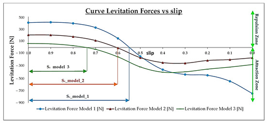
Figure 5. Characteristic curve levitation force versus slip.

From this analysis, we obtain one of the most important conclusions of this paper. At the beginning of the simulations, the thrust force developed by the machine and the levitation force evolves inversely as we add geometric modifications in Models 2 and 3. The changes in the geometry imply a substantial improvement in the thrust force but a decrease in the levitation force. The geometric changes also imply a modification of S_c; $S_{c\_Model\_3}>S_{c\_Model\_2}>S_{c\_Model\_1}$. Model 1 has a S_c value of around 0.55 (in this case, TFLIM only operates with transverse magnetic flux). Model 2 shows a higher value, around 0.6, and Model 3 shows around 0.7 (this motor operates with mixed magnetic flux). The increase in the value of S_c implies a reduction in the speed with which the TFLIM loses levitation conditions; therefore, the attractive forces become dominant in the motor. This change is mainly observed after the inclusion of the ferromagnetic stator yoke under the central tooth of the primary part of the linear motor.

Finally, after each configuration exceeded the characteristic value of S_c, the attractive forces showed very significant values as we approached slips close to zero or, in other words, speeds close to the synchronous speed. At this point, it is important to highlight that the repulsive force of Model 1 is always higher than Model 2 and Model 3. In addition, the attractive force in Model 1 is the highest (−747.633 N) when the linear motor operates at a synchronous speed. Consequently, the proposed geometric changes contribute to attenuating the predominant attractive effect when Model 1 operates at high speeds close to slips between 0.3 and 0. In this region, the behaviour of the attractive forces can be observed according to the following trend ${\overrightarrow{F}}_{z\_Model\_1}>{\overrightarrow{F}}_{z\_Model\_3}>{\overrightarrow{F}}_{z\_Model\_2}$.

5. Indirect Test Results

In this section, we show the indirect test simulation results carried out with FEM-3D (these tests are usually used in RIM). Firstly, we present the main conclusions about the blocked secondary tests, and, secondly, we present the conclusions about the no load tests [22,23,24,25]. We always work under an unbalanced current system, so the equations presented in this section use the values of the electrical currents of each phase obtained from the tests [26]. We will also compare the main differences between the three proposed TFLIM models and evaluate the effects of the changes made to the geometry to compute the EC parameters. Figure 6 shows the output from indirect tests obtained by FEM 3-D.

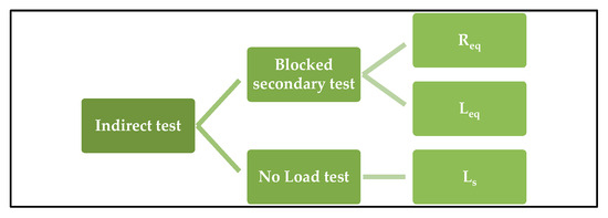
Figure 6. Scheme of indirect test simulation in FEM-3D.

5.1. Blocked Secondary Tests: Estimation of $R_{eq}$ and $L_{eq}$

This subsection describes the simulation of the TFLIM models under standstill conditions or secondary part blockages, where the motion of the moving part is equal to zero, $v_{sec}=0 \mathrm{m}/\mathrm{s}$. The range of frequencies to the simulations in FEM-3D is shown in Table 3. $f_{supply}$ (Hz) corresponds to the frequency linked to the voltage source that supplies the TFLIM (from 55 Hz. to 100 Hz). To correctly simulate the TFLIM models, it is necessary to establish three characteristic times (see Equations (5)–(7)). $T_{cycle} (\mathrm{m}\mathrm{s})$ is the cycle time of the sinusoidal wave generated by the voltage source, $T_{simulation} (\mathrm{m}\mathrm{s})$ is the number of cycles necessaries to complete the simulation, and $T_{sample} (\mathrm{m}\mathrm{s})$ is the time slot adequate to achieve a convergence solution in FEM-3D [8].

$$T_{simulation}=3·T_{cycle}$$

(5)

$$T_{sample}=\raisebox{1ex}{$T_{cycle}$}\!\left/ \!\raisebox{-1ex}{$10$}\right.$$

(6)

$$T_{cycle}=\raisebox{1ex}{$1$}\!\left/ \!\raisebox{-1ex}{$f_{supply}$}\right.$$

(7)

Table 3. Frequencies and main times used in FEM-3D under standstill conditions.

Characteristic Times for Simulating Blocked Tests in FEM-3D
fsupply_sh (Hz)	Tcycle (ms)	Tsimulation (ms)	Tsample (ms)
55	18.182	54.545	1.818
60	16.667	50.000	1.667
70	14.286	42.857	1.429
80	12.500	37.500	1.250
90	11.111	33.333	1.111
100	10.000	30.000	1.000

The estimation of equivalent resistance and inductance needs the measurement of active and reactive powers obtained by FEM-3D. We use the following nomenclature to explain the estimation:

1.

The following equations contain the sub-index $i$, which indicates the type of TFLIM topology used. So, $i=1$, corresponds to Model 1, $i=2$ (Model 2), and $i=3$ (Model 3). This is very useful to differentiate the types of powers consumed by the models.

2.

Also, we use the abbreviations ‘$sh$’ to indicate ‘short-circuit’ (in tests under standstill conditions) and ‘o’ with the no-load test, which corresponds to ‘open-circuit’ TFLIM configuration. Then, we adapted the classic nomenclature used in RIM to TFLIM tests carried out with FEM-3D.

To estimate the equivalent resistance, $R_{eq}(\Omega )$, we use the measurement of the active power of each phase according to Equation (8), where $P_{sh\_a\_Model\_i}(\mathrm{W})$ is the active power consumed by phase A, $P_{sh\_b\_Model\_i}(\mathrm{W})$ is linked to phase B and $P_{sh\_c\_Model\_i} (\mathrm{W})$ is the active power consumed by phase C. After we obtained each active power, we used the variable $P_{sh\_Tot\_Model\_i }(\mathrm{W})$ to consider the contribution of all. $i_{sh\_a\_Model\_i} (\mathrm{A})$, $i_{sh\_b\_Model\_i} (\mathrm{A})$ and $i_{sh\_c\_Model\_i} (\mathrm{A})$ are the electric current per phase obtained under standstill conditions. Consequently, $R_{eq\_Model\_i}(\Omega )$ can be obtained from Equation (8).

Now, we want to estimate $L_{eq} (\mathrm{H})$. For this purpose, we measure the reactive power per phase according to Equation (9), where $Q_{sh\_a\_Model\_i}(\mathrm{K}\mathrm{V}\mathrm{A}\mathrm{r}),$ $Q_{sh\_b\_Model\_i}(\mathrm{K}\mathrm{V}\mathrm{A}\mathrm{r}),$ and $Q_{sh\_c\_Model\_i} (\mathrm{K}\mathrm{V}\mathrm{A}\mathrm{r})$ are the reactive power consumed by phase A, phase B, and phase C, respectively. In this case $Q_{sh\_Tot\_Model\_i }(\mathrm{K}\mathrm{V}\mathrm{A}\mathrm{r})$ represents the total reactive power for model i and $X_{eq\_Model\_i}(\Omega )$ represents the equivalent reactance per phase. Using Equation (10), equivalent inductance $L_{eq\_Model\_i }(\mathrm{H})$ is obtained for each TFLIM using the values of $f_{supply\_sh}(\mathrm{H}\mathrm{z})$ attached in Table 3.

Active powers:

$$\begin{gathered} P_{s{h}_{To{t}_{Mode{l}_i}}}=P_{s{h}_{A_{Mode{l}_i}}}+P_{s{h}_{B_{Mode{l}_i}}}+P_{s{h}_{C_{Mode{l}_i}}}= \\ \left(i_{sh\_a\_Model\_i}^2+i_{sh\_b\_Model\_i}^2+i_{sh\_c\_Model\_i}^2\right)·R_{eq\_Model\_i} \end{gathered}$$

(8)

Reactive powers:

$$\begin{gathered} Q_{s{h}_{To{t}_{Mode{l}_i}}}=Q_{s{h}_{a_{Mode{l}_i}}}+Q_{s{h}_{b_{Mode{l}_i}}}+Q_{s{h}_{c_{Mode{l}_i}}}= \\ \left(i_{sh\_a\_Model\_i}^2+i_{sh\_b\_Model\_i}^2+i_{sh\_c\_Model\_i}^2\right)·X_{e{q}_{Mode{l}_i}} \end{gathered}$$

(9)

$$L_{eq\_Model\_i}=\raisebox{1ex}{$X_{eq\_Model\_i}$}\!\left/ \!\raisebox{-1ex}{${\omega }_e$}\right.=\raisebox{1ex}{$X_{eq\_Model\_i}$}\!\left/ \!\raisebox{-1ex}{$2·\pi ·f_{supply}$}\right.$$

(10)

Results from Indirect Test under Standstill Conditions

Now, we study the results from tests under standstill conditions. Figure 7 shows the evolution of $R_{eq}$ and $L_{eq}$ along the selected range of frequencies. From this figure, we can obtain the following conclusions:

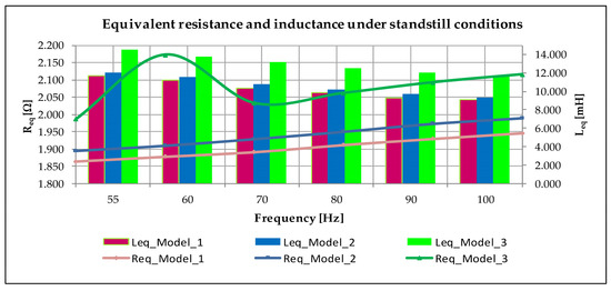
Figure 7. $R_{eq}$ and $L_{eq}$ values obtained under standstill conditions.

• The behaviour of R_eq is $R_{eq\_Model\_1}\le R_{eq\_Model\_2}\le R_{eq\_Model\_3}$ in all tests simulated. The inclusion in Model 2 of non-ferromagnetic slots and a new ferromagnetic yoke does not imply a relevant increase in $R_{eq}$. So, if we compare Model 1 and Model 2, we can observe that the difference between both models is insignificant. When we work at 100 Hz, $R_{eq\_Model\_1}=1.9465 \Omega$ and $R_{eq\_Model\_2}=1.9898 \Omega$, so the addition of two non-conducting slots inside the aluminium layer does not influence the estimation of $R_{eq}$. However, if we consider Model 3, we obtain slightly higher results than previous models (with 100 Hz $R_{eq\_Model\_3}=2.1154 \Omega$). In Model 3, the addition of the new ferromagnetic yoke in the primary located below the central transverse tooth implies a new volume of steel of 2,089,525 mm³. This new element increases the total resistance of the equivalent circuit under conditions of blocked secondary. This is validated with the six tests conducted, where $R_{eq\_Model\_3}>R_{eq\_Model\_2}>R_{eq\_Model\_1}$. The second test is carried out at 60 Hz, where $R_{eq\_Model\_3}$ presents a slightly higher value than expected, resulting in the deviation from the linear behaviour of the equivalent resistance. A value approximately only 0.150 mΩ higher than expected is obtained, but these atypical data do not have a significant impact on the calculation of the total equivalent impedance in which $R_{eq}<X_{eq}$.
• $L_{eq\_Model\_1}<L_{eq\_Model\_2}<L_{eq\_Model\_3}$ is the trend obtained in all tests simulated. Model 3 presents values higher than other models. With a frequency of 55 Hz, $L_{eq}$ reaches the maximum value in all models ($L_{eq\_Model\_3}=14.348 \mathrm{m}\mathrm{H}$, $L_{eq\_Model\_2}=11.936 \mathrm{m}\mathrm{H}$, $L_{eq\_Model\_1}=11.593 \mathrm{H}$). A new useful magnetic flux along the longitudinal direction circulates through Model 3, and consequently, the current required for the magnetization of the machine is lower mainly because the longitudinal slot leakage flux was eliminated. This phenomenon results in the logical evolution achieved during the tests where $L_{eq\_Model\_1}<L_{eq\_Model\_2}<L_{eq\_Model\_3}$. Notice that Hopkinson’s law [8] indicates that $L=\raisebox{1ex}{$N^2$}\!\left/ \!\raisebox{-1ex}{$\mathfrak{R}$}\right.$, (L: inductance, N: number of turns, and R: reluctance), so that the new ferromagnetic yoke implies a decrease in the reluctance of the equivalent magnetic circuit and, consequently, an increase in the value of inductance.
• Figure 8 represents the equivalent reactance $X_{eq}(\Omega )$ and the equivalent impedance $Z_{eq}(\Omega )$ for each model under standstill conditions. Both parameters can be computed by Equations (11) and (12), respectively [9]. $Z_{eq}$ is equal to the module value of $Z_{eq}$ that is given by the root square of $R_{eq}$ and $X_{eq}$. With the changes that we have added to the geometry, $Z_{eq}$ increase, so $Z_{eq\_Model\_3}<Z_{eq\_Model\_2}<Z_{eq\_Model\_1}$ and all tests carried out give us similar results. Additionally, it is important to highlight the predominance of $X_{eq}$ in comparison with $R_{eq}$, so we can establish $X_{eq}>R_{eq}$.

  $$X_{eq}=2·\pi ·f_{suppl{y}_{sh}}·L_{eq}$$

  (11)

  $$Z_{eq}=R_{eq}+j·X_{eq}⟹\left|Z_{eq}\right|=\sqrt{{R_{eq}}^2+{X_{eq}}^2}$$

  (12)
  

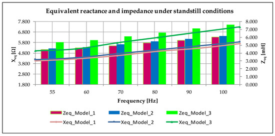  Figure 8. $X_{eq}$ and $Z_{eq}$ values obtained under standstill conditions.
• Finally, the variation in the excitation frequency throughout the proposed tests must be considered. Thus, when computing $X_{eq}$, two opposing effects occur. It is observed that as the frequency increases in the tests $f_{supply\_sh}\uparrow$, the value of $L_{eq\_Model\_3}\downarrow$ decreases throughout the tests, so the product of both results in an evolution of $Z_{eq}$ and $X_{eq}$ opposite to $L_{eq}$.

To complete the analysis of the obtained results from tests under standstill conditions, we computed the average values of active power, $\overline{P_{sh\_Model\_i}}(\mathrm{K}\mathrm{W})$ and reactive power, $\overline{Q_{sh\_Model\_i}} (\mathrm{K}\mathrm{V}\mathrm{A}\mathrm{r})$ consumed by each model (see Equations (13) and (14)). In Electrical Engineering, it is usual to work with per-phase values, so Figure 9 focuses on the average active and reactive power per phase in each test. The presence of a non-equilibrated three-phase system is a phenomenon inherent to TFLIM due to the finite length of the primary part. This phenomenon is known as the static longitudinal edge effect (${LEE}_{static}$), and it is determined by the relative position of each phase of the stator winding in the motor’s primary. This effect will be accentuated by the four-layer winding designed with the finite element tool.

$$\overline{P_{sh\_Model\_i}}=\raisebox{1ex}{$\left(P_{sh\_a\_Model\_i}+P_{sh\_b\_Model\_i}+P_{sh\_c\_Model\_i}\right)$}\!\left/ \!\raisebox{-1ex}{$3$}\right.$$

(13)

$$\overline{Q_{sh\_Model\_i}}=\raisebox{1ex}{$\left(Q_{sh\_a\_Model\_i}+Q_{sh\_b\_Model\_i}+Q_{sh\_c\_Model\_i}\right)$}\!\left/ \!\raisebox{-1ex}{$3$}\right.$$

(14)

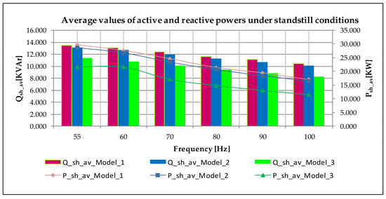
Figure 9. Averages values of active and reactive powers of each TFLIM model.

5.2. No Load Tests Estimation of $L_s$

The goal of this test is to estimate the primary part inductance, $L_s (\mathrm{H})$. To simulate it correctly, we follow two steps: firstly, we avoid the effect of the secondary part, so the simulations must be executed with a slip equal to zero (the absence of relative motion implies a reduction in the eddy currents induced inside the aluminium layer); secondly, for these tests, the selected range of frequencies must reduce the end effect phenomenon (see Table 4). Now, using Equation (15), the primary reactance of each TFLIM model, $X_{s\_Model\_i} (\Omega )$ can also be estimated. $Q_{o\_a\_Model\_i }(\mathrm{K}\mathrm{V}\mathrm{A}\mathrm{r})$, $Q_{o\_b\_Model\_i} (\mathrm{K}\mathrm{V}\mathrm{A}\mathrm{r})$ and $Q_{o\_c\_Model\_i} (\mathrm{K}\mathrm{V}\mathrm{A}\mathrm{r})$ are the reactive power in phases A, B, and C, respectively. $Q_{o\_Tot\_Model\_i }(\mathrm{K}\mathrm{V}\mathrm{A}\mathrm{r})$ is the total reactive power absorbed. Primary part inductance is computed using Equation (16), which includes the selected range of frequencies for these tests, called $f_{supply\_o} (\mathrm{H}\mathrm{z}).$

$$\begin{gathered} Q_{o\_Tot\_Model\_i }=Q_{o\_a\_Model\_i }+Q_{o\_b\_Model\_i }+Q_{o\_c\_Model\_i }= \\ \left(i_{o\_a\_Model\_i}^2+i_{o\_b\_Model\_i}^2+i_{o\_c\_Model\_i}^2\right)·X_{s\_Model\_i} \end{gathered}$$

(15)

$$L_{s\_Model\_i}=\raisebox{1ex}{$X_{s\_Model\_i}$}\!\left/ \!\raisebox{-1ex}{${\omega }_e$}\right.=\raisebox{1ex}{$X_{s\_Model\_i}$}\!\left/ \!\raisebox{-1ex}{$2·\pi ·f_{supply\_o}$}\right.$$

(16)

Table 4. Frequencies and main times used in FEM-3D under standstill conditions.

Characteristic Times for Simulating no Load Tests in FEM-3D
fsupply_o (Hz)	Tcycle (ms)	Tsimulation (ms)	Tsample (ms)	Vsec (m/s)
18	55.556	166.667	5.556	7.2
16	62.500	187.500	6.250	6.4
14	71.429	214.286	7.143	5.6
12	83.333	250.000	8.333	4.8
10	100.000	300.000	10.000	4
8	125.000	375.000	12.500	3.2

Results from Indirect Test under No Load Conditions

Figure 10 shows the values of $L_s$. We can see that $L_{s\_Model\_3}>L_{s\_Model\_2}>L_{s\_Model\_1}$. This behaviour is similar in all proposed tests. Therefore, the central ferromagnetic yoke added below the central teeth implies an increase in the primary part inductance. If we analyse data from 8 Hz in Model 3, $L_s$ reaches 50.770 mH, while in Model 1 and Model 2, the values are very close to each other (47.03 mH and 47.8 mH). Additionally, to complete the whole analysis of the indirect tests, we incorporate, in Figure 10, the primary impedance ${\mathrm{Z}}_s(\Omega )$ obtained under no load conditions. It computed following Equations (17) and (18), where $f_{supply\_o}$ data are in Table 4. To obtain the primary impedance, we calculate the equivalent resistance per phase, $R_s (\Omega )$, using Equation (19). There, a set of variables that describe some constructive aspects of the primary winding is described: ${\overline{L}}_{coil} (\mathrm{m}\mathrm{m})$ is the average length of a single coil with a value of 526.5 mm, ${\rho }_{Cu}(\Omega ·{\mathrm{m}\mathrm{m}}^2/\mathrm{m})$ is the conductivity of the copper wire with a value of 2$.37·{10}^{-2}$, $n_{phase}$ is equal to 8 (the number of coils per phase),$A_c$(mm²) is the cross-sectional area of the conductor equal to 1.7, and $N_{phase}$ is the number of turns per phase equal to 22 turns.

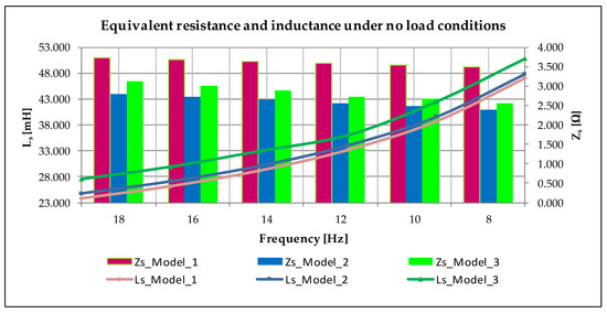
Figure 10. $L_s$ and $Z_s$ values obtained under no load conditions.

The evolution of ${\mathrm{Z}}_s$ diverges from $L_s$ so $Z_{s\_Model\_1}>Z_{s\_Model\_3}>Z_{s\_Model\_2}$. Model 1 presents the highest value, around 3.6 Ω at 18 Hz. In Model 2, $Z_s$ presents the lowest value with 2.3 Ω approximately, so this TFLIM is the optimum configuration with respect to the primary part resistance. In conclusion, using no load tests, we checked the convenience of modifying the initial TFLIM (model 1) because in Models 2 and 3, $Z_s$ decreases.

$$Z_s=R_s+j·X_s⟹\left|Z_s\right|=\sqrt{{R_s}^2+{X_s}^2}$$

(17)

$$X_s=2·\pi ·f_{supply\_o}·L_s$$

(18)

$$R_s=\raisebox{1ex}{$n_{phase}·\left({\rho }_{Cu}·{\overline{L}}_{coil}·N_{phase}\right)$}\!\left/ \!\raisebox{-1ex}{$A_c$}\right.$$

(19)

Figure 11 shows the average value of the reactive power consumed by each TFLIM topology; $\overline{Q_{o\_av\_Model\_i}}(\mathrm{K}\mathrm{V}\mathrm{A}\mathrm{r})$ is calculated using Equation (20), where $Q_{o\_a\_Model\_i} (\mathrm{K}\mathrm{V}\mathrm{A}\mathrm{r})$, $Q_{o\_b\_Model\_i }(\mathrm{K}\mathrm{V}\mathrm{A}\mathrm{r}),$ and $Q_{o\_c\_Model\_i}(\mathrm{K}\mathrm{V}\mathrm{A}\mathrm{r})$ are the reactive power per phase. To complete no load tests, we use the electric current consumed $\overline{i_{o\_av\_Model\_i}(}\mathrm{A})$. See Equation (21), where $i_{o\_a\_Model\_i}$(A), $i_{o\_b\_Model\_i}$(A), and $i_{o\_c\_Model\_i}$(A) are the electric current absorbed by each phase. Basically, $\overline{Q_{o\_Model\_i}}$ and $i_{o\_av\_Model\_i}$ have a very similar trend because $Q_{o\_av\_Model\_3}<Q_{o\_av\_Model\_2}<Q_{o\_av\_Model\_1}$ and $i_{o\_av\_Model\_3}<i_{o\_av\_Model\_2}<i_{o\_av\_Model\_1}$.

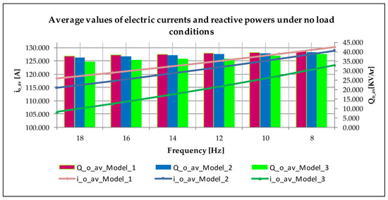
Figure 11. Average reactive powers and electric currents absorbed under no load conditions.

The results obtained with no load tests determine the convenience of the new TFLIM configurations. We not only achieved an improvement in $Z_s$ but also $\overline{Q_{o\_av}}$ and $\overline{i_{o\_av}}$ decreases when we incorporate the changes in Models 2 and 3.

$$\overline{Q_{o\_Model\_i}}=\raisebox{1ex}{$\left(Q_{o\_a\_Model\_i}+Q_{o\_b\_Model\_i}+Q_{o\_c\_Model\_i}\right)$}\!\left/ \!\raisebox{-1ex}{$3$}\right.$$

(20)

$$\overline{i_{o\_av\_Model\_i}}=\raisebox{1ex}{$\left(i_{o\_a\_Model\_i}+i_{o\_b\_Model\_i}+i_{o\_c\_Model\_i}\right)$}\!\left/ \!\raisebox{-1ex}{$3$}\right.$$

(21)

6. System of Equations Used to Determine the Electric Parameters to the Equivalent Circuit

Here, we describe the system of equations proposed to obtain the EC parameters [23,27,28,29,30]. Table 5 shows the set of variables involved in our system, and the details of the different equations are as follows:

Table 5. Classification of the parameters involved in the system of equations proposed.

Scheme of Parameters Involved in EC Parameters Estimation
Classification of the Variables in the System of Equations				Frequency Simulation (Hz)
Variables Obtained by FEM-3D		Defined Variables	Unknown Variables	Test 1	Test 2	Test 3	Test 4	Test 5	Test 6
Standstill test	${\mathrm{R}}_{\mathrm{e}\mathrm{q}}(\Omega )$ ${\mathrm{L}}_{\mathrm{e}\mathrm{q}}(\mathrm{H})$	${\omega }_2(\raisebox{1ex}{$\mathrm{r}\mathrm{a}\mathrm{d}$}\!\left/ \!\raisebox{-1ex}{$\mathrm{s}$}\right.)$ ${\tau }_p(\mathrm{m}\mathrm{m})$ $L(\mathrm{m}\mathrm{m})$ $\beta$	$L_m(\mathrm{H})$	55	60	70	80	90	100
			$L_r(\mathrm{H})$
No load test	${\mathrm{L}}_{\mathrm{S}}(\mathrm{H})$		$R_r(\Omega )$	18	16	14	12	10	8
Nominal conditions	${\mathrm{F}}_{\mathrm{y}}(\mathrm{N})$ ${\mathrm{I}}_{\mathrm{s}}(\mathrm{A})$		$I_2(\mathrm{A})$	50
			$I_m(\mathrm{A})$

• Equivalent Resistance equation: Equation (22) calculates the $R_{eq}$ of the indirect tests, where $R_s(\Omega )$ is the primary resistance, $R_r (\Omega )$ the secondary resistance, $L_m (\mathrm{H})$ the magnetizing inductance,$L_r(\mathrm{H})$ the secondary inductance and ${\omega }_e (\raisebox{1ex}{$\mathrm{r}\mathrm{a}\mathrm{d}$}\!\left/ \!\raisebox{-1ex}{$\mathrm{s}$}\right.)$ the angular frequency.

  $${R_{eq}=R}_s+\left(\raisebox{1ex}{${\omega }_e^2·L_m^2·R_r$}\!\left/ \!\raisebox{-1ex}{$R_r^2+{\omega }_e^2·L_r^2$}\right.\right)$$

  (22)
• Equivalent Inductance equation: Equation (23) defines the $L_{eq} (\mathrm{H})$, the equivalent inductance obtained under standstill conditions.

  $${L_{eq}=L}_s-L_m+\left(\raisebox{1ex}{$\left(L_m·\left[R_r^2+{\omega }_e^2·L_r·\left(L_r-L_m\right)\right]\right)$}\!\left/ \!\raisebox{-1ex}{$\left(R_r^2+{\omega }_e^2·L_r^2\right)$}\right.\right)$$

  (23)
• Inductance Quotient equation: The dimensionless parameter $\beta$ obtained with Equation (24) is the quotient between the magnetizing inductance and secondary inductance.

  $$\beta =\raisebox{1ex}{$L_m$}\!\left/ \!\raisebox{-1ex}{$L_r$}\right.$$

  (24)
• Thrust Force equation: Equation (25) uses three categories of thrust forces: $F_y (\mathrm{N})$ that represents the net thrust force generated, $F_{y1}(\mathrm{N})$ that represents the thrust force produced by the slip current, and $F_{y2}(\mathrm{N})$ that represents the thrust force produced by the demagnetizing loss. In addition, $L=503.5 \mathrm{m}\mathrm{m}$ is the TFLIM length, $L_{lr} (\mathrm{H})$ the secondary leakage inductance, ${\omega }_2 (\mathrm{r}\mathrm{a}\mathrm{d}/\mathrm{s})$ the secondary angular frequency and ${\tau }_p(\mathrm{m}\mathrm{m})=200$ the pole pitch.

  $$F_y=F_{y1}-F_{y2}=\left(3·I_2^2·R_r·\raisebox{1ex}{$\pi $}\!\left/ \!\raisebox{-1ex}{${\omega }_2·{\tau }_p$}\right.\right)-\left(\raisebox{1ex}{$3·I_m^2\left(L_m+L_{lr}\right)$}\!\left/ \!\raisebox{-1ex}{$L$}\right.\right)$$

  (25)
• Electric Current equation: Equation (26) establishes the relationship between the main electric currents. $I_s(\mathrm{A})$ is the electric current consumed by the voltage source, $I_{2 }(\mathrm{A})$ is the secondary electrical current per phase, and $I_m$ (A) is the magnetizing current per phase. It is important to denote that to obtain $I_s$, the electric current absorbed by each phase using Equation (27) is considered, where $I_{phase\_a}$ (A),$I_{phase\_b},$ and $I_{phase\_c}$ (A) are the electric currents in each phase obtained with FEM 3-D under nominal conditions.

  $$I_s=I_m+I_2$$

  (26)

  $$I_s=\raisebox{1ex}{$\left(I_{phase\_a}+I_{phase\_b}+I_{phase\_c}\right)$}\!\left/ \!\raisebox{-1ex}{$3$}\right.$$

  (27)

Additionally, Equations (28) and (29) must be considered, where primary inductance $L_s(\mathrm{H})$ and secondary inductance $L_r (\mathrm{H})$ depend on the primary leakage inductance,$L_{ls}(\mathrm{H})$ and secondary leakage inductance, $L_{lr} (\mathrm{H}),$ respectively.

$${\mathrm{L}}_{\mathrm{s}}={\mathrm{L}}_{\mathrm{m}}+{\mathrm{L}}_{\mathrm{l}\mathrm{s}}$$

(28)

$$L_r=L_m+L_{lr}$$

(29)

Section 6.1 describes the results of magnetization inductance and compares the results obtained from different models. In Section 6.2, an analysis of the primary leakage inductance and its evolution among the proposed topologies is detailed. Next, in Section 6.3, the secondary parameters of the equivalent circuit are examined, starting with the secondary leakage inductance. In Section 6.4, the equivalent resistance of the secondary is analysed. Finally, Section 6.5 describes a qualitative analysis of thrust force in TFLIM according to electric parameters.

6.1. Magnetizing Inductance Analysis, L_m

It is very important to explain the values of magnetizing inductance $L_m$ and magnetizing reactance $X_m$ that we obtained with the method proposed. In [9], a comprehensive mathematical development is undertaken to obtain the magnetization inductance through two alternative methods in order to validate the process designed in the present research. One method is focused on the value of the main harmonic of the magnetic field density along the air gap $B_{\delta \_max}$(T) of Model 1 that is taken as the starting point. Through this mathematical proposal, a value of $L_{\mathrm{m}}=12.789 \mathrm{m}\mathrm{H}$ is obtained. The other method is described in the present article, where the mean value of $L_{\mathrm{m}}$ across the six designed tests, gives a value of $L_{\mathrm{m}}=12.283 \mathrm{m}\mathrm{H}$. A high correlation between both results can be verified.

In Figure 12, the y-axis on the left shows the magnetizing inductance values and, on the right, the magnetizing reactance. $L_{m\_Model\_1} (\mathrm{m}\mathrm{H})$, $L_{m\_Model\_2} (\mathrm{m}\mathrm{H})$ and $L_{m\_Model\_3} (\mathrm{m}\mathrm{H})$ are the magnetizing inductances for Model 1, Model 2, and Model 3, respectively. ${\chi }_{m\_Model\_1}(\Omega )$, ${\chi }_{m\_Model\_2}(\Omega ),$ and ${\chi }_{m\_Model\_3}(\Omega )$ are the magnetizing reactance of each TFLIM model. We compared both parameters between the three TFLIM models. To this end, we defined a quotient to quantify the advantage that implies each geometrical change introduced into the geometry. Therefore:

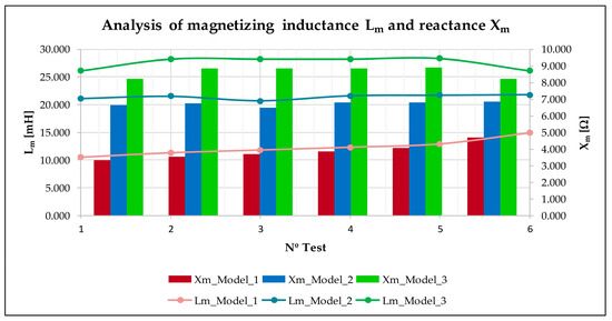
Figure 12. Magnetizing inductance and reactance to each TFLIM model.

• Figure 12 shows that $L_{m\_Model\_3}>L_{m\_Model\_2}>L_{m\_Model\_1}$. An important consequence is obtained from these values because we can translate the advantage from adding changes into the TFLIM geometry to the EC parameters. All tests carried out give us a similar behaviour with the magnetizing reactance ${\chi }_{m\_Model\_3}>{\chi }_{m\_Model\_2}>{\chi }_{m\_Model\_1}$. The magnetizing reactance is located inside our EC model into the parallel branch; an increment in this inductive impedance implies a reduction of the magnetizing current; that is to say, the secondary current available to generate the thrust force is increased. Equations (30) and (31) determine the improvement between the TFLIM models (see Table 6). $\Delta {\mathrm{L}}_{\mathrm{m}}^{2-1}(\mathrm{\%})$ represents the percentual change in the magnetizing inductance between Model 1 and Model 2 while $\Delta {\mathrm{L}}_{\mathrm{m}}^{3-2}(\mathrm{\%})$ represents this value between Model 2 and Model 3.
  Table 6. Values related to specific gain Λ_Lm.

  Lm (mH)
  Nº Test	TFLIM Models			Variation (%)		Gain: ΛLm (mH/N)
  	Model 1	Model 2	Model 3	∆ Lls2−1	∆ Lls3−2	ΛLls2−1	ΛLls3−2
  Test 1	10.500	21.100	26.100	50.237	19.157	2.553	0.729
  Test 2	11.300	21.500	28.200	47.442	23.759	2.411	0.904
  Test 3	11.800	20.700	28.200	42.995	26.596	2.185	1.012
  Test 4	12.300	21.600	28.200	43.056	23.404	2.188	0.890
  Test 5	12.900	21.700	28.300	40.553	23.322	2.061	0.887
  Test 6	14.900	21.800	26.100	31.651	16.475	1.609	0.627

For Model 2, the addition of two non-ferromagnetic slots supposes an increment of $\Delta L_m^{2-1}$ that changes from 50% (Test 1) to 30% (Test 6). This result is very relevant because this configuration of the aluminium layer allows the TFLIM to operate with three inner motors. In this way, central and lateral teeth generate the trust force, and all magnetic flux works to develop a force along the direction of the movement [8]. The inclusion of a central ferromagnetic yoke in Model 3 sets up the magnetic circuit, so a longitudinal magnetic flux operates into the machine and generates a positive thrust force. In Test 1, $\Delta {\mathrm{L}}_{\mathrm{m}}^{3-2}$ increases around 19%, and it decreases at 16% for Test 6.

$$\Delta L_m^{2-1}(\mathrm{\%})=\left(\raisebox{1ex}{$L_{m\_Model\_2}-L_{m\_Model\_1}$}\!\left/ \!\raisebox{-1ex}{$L_{m\_Model\_2}$}\right.\right)·100$$

(30)

$$\Delta L_m^{3-2}(\mathrm{\%})=\left(\raisebox{1ex}{$L_{m\_Model\_3}-L_{m\_Model\_2}$}\!\left/ \!\raisebox{-1ex}{$L_{m\_Model\_3}$}\right.\right)·100$$

(31)

• The mean value of the magnetizing inductance for each model is a value around 12.13 mH for Model 1, 21.39 mH for Model 2, and 27.48 mH for Model 3. These values are estimated using Equations (32)–(34), where $\overline{L_{m\_Model\_1}} (\mathrm{m}\mathrm{H})$, $\overline{L_{m\_Model\_2}}(\mathrm{m}\mathrm{H}),$ and $\overline{L_{m\_Model\_3}}(\mathrm{m}\mathrm{H})$ are the mean value of the magnetizing inductance in each case, and $n=6$ is the number of tests simulated.

  $$\overline{L_{m_{Mode{l}_1}}}=\sum _{n=1}^6{L}_{m_{Mode{l}_1}}^n/n$$

  (32)

  $$\overline{L_{m_{Mode{l}_2}}}=\sum _{n=1}^6{L}_{m_{Mode{l}_2}}^n/n$$

  (33)

  $$\overline{L_{m\_Model\_3}}=\sum _{n=1}^6{L}_{m\_Model\_3}^n/n$$

  (34)
• Now, we propose a new KPI that helps to evaluate prototypes. Usually, electrical engineers work with goodness factor or efficiency ratio, but we define an intermediate quotient that allows us to incorporate the contribution of each geometrical change into the net thrust force developed. ${\Lambda }_{L_m}(\mathrm{m}\mathrm{H}/\mathrm{N})$ is the gain of the inductance that considers the ratio between the increment of the magnetizing inductance and the net thrust force generated (see Equation (35)). The index i−j denotes the model. The values of these coefficients are shown in Table 6.

  $${\Lambda }_{L_m}^{i-j}={\left(\raisebox{1ex}{$\Delta L_m$}\!\left/ \!\raisebox{-1ex}{$\Delta F_y$}\right.\right)}_{i-j}$$

  (35)

Using Equation (35) for Model 2, we obtain a gain ${\Lambda }_{{\mathrm{L}}_{\mathrm{m}}}^{2-1}$ that varies between 2.55 mH/N (Test 1) and 1.61 mH/N (Test 6). ${\Lambda }_{{\mathrm{L}}_{\mathrm{m}}}^{3-2}$ measures the gain once we added the central ferromagnetic yoke, and it was lower than ${\Lambda }_{{\mathrm{L}}_{\mathrm{m}}}^{2-1}$ (varies from 0.73 (Test 1) to 0.63 (Test 6)). So, we can conclude the following three statements about the magnetizing inductance analysis:

1.

Firstly, $\Delta {\mathrm{L}}_{\mathrm{m}}^{2-1}>0$ and $\Delta L_m^{3-2}>0$ allows us to quantify the convenience of adding geometric changes in the TFLIM considering the value of the EC parameter. The modifications made in the primary and secondary parts are included in the magnetizing inductance where $\Delta {\mathrm{L}}_{\mathrm{m}}^{2-1}>\Delta L_m^{3-2}$.

2.

Secondly, all tests proposed indicate the same results that we obtain analysing the mean value of the magnetizing inductance: $\overline{L_{m\_Model\_1}}<\overline{L_{m\_Model\_2}}<\overline{L_{m\_Model\_3}}$.

3.

Thirdly, we defined a gain to evaluate the improvement of $L_m$ and to compare with the net thrust force developed. We obtained ${\Lambda }_{{\mathrm{L}}_{\mathrm{m}}}^{2-1}>0$ and ${\Lambda }_{{\mathrm{L}}_{\mathrm{m}}}^{3-2}>0$ and verified that ${\Lambda }_{{\mathrm{L}}_{\mathrm{m}}}^{2-1}>{\Lambda }_{{\mathrm{L}}_{\mathrm{m}}}^{3-2}$.

6.2. Primary Leakage Inductance, L_ls

The next step is to determine the primary leakage inductance $L_{ls}$ for the TFLIM models. It is important to remark that $L_{ls }(\mathrm{m}\mathrm{H})$ is the result of the addition of magnetic leakage fluxes that do not reach the secondary part [27]. Additionally, the air gap flux space harmonics produce a primary part electromotive force (EMF), so it should also be considered in the leakage category. Now, we only analyse total leakage flux. Figure 13 represents the $L_{ls}$ values obtained for each model. $L_{l{s}_{Mode{l}_1}}(\mathrm{m}\mathrm{H}),$ $L_{ls\_Model\_2} (\mathrm{m}\mathrm{H})$ and $L_{ls\_Model\_3}(\mathrm{m}\mathrm{H})$ are the $L_{ls}$ data obtained for each model in the tests proposed previously.

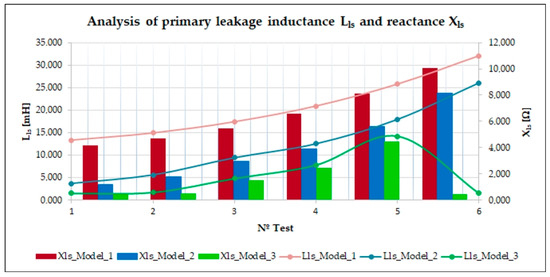
Figure 13. Primary leakage inductance and reactance obtained in each TFLIM model.

Model 1 operates under transverse magnetic flux conditions, and only the central teeth contribute to generating a thrust force along the desired direction. In Model 2, all transverse magnetic fluxes produce an effective electromagnetic conversion, so the $L_{ls}$ will be lower than Model 1. Finally, Model 3 must present the lowest $L_{ls}$ value. Figure 13 also represents the associated reactance values, ${\mathrm{X}}_{ls}(\Omega )$ (${\mathrm{X}}_{ls\_Model\_1}(\Omega )$, ${\mathrm{X}}_{ls\_Model\_1}(\Omega )$, and ${\mathrm{X}}_{ls\_Model\_3}(\Omega )$ are reactance data for each model). Finally, in a similar way that $L_m$, we define a new KPI to describe the evolution of $L_{ls}$ with the net thrust force, ${\Lambda }_{L_{ls}}(\mathrm{m}\mathrm{H}/\mathrm{N})$, (see Equation (36)). Table 7 shows the values of $L_{ls}$, ${\mathrm{X}}_{ls}$, and ${\Lambda }_{{\mathrm{L}}_{\mathrm{l}\mathrm{s}}}^{\mathrm{i}-\mathrm{j}}$.

$${\Lambda }_{L_{ls}}^{i-j}={\left(\raisebox{1ex}{$\Delta L_{ls}$}\!\left/ \!\raisebox{-1ex}{$\Delta F_y$}\right.\right)}_{i-j}$$

(36)

Table 7. Values related to specific gain Λ_Lls.

Lls (mH)
Nº Test	TFLIM Models			Variation (%)		Gain: ΛLls (mH/N)
	Model 1	Model 2	Model 3	∆ Lls2−1	∆ Lls3−2	ΛLls2−1	ΛLls3−2
Test 1	13.300	3.700	1.500	72.180	59.459	0.488	0.084
Test 2	14.900	5.600	1.700	62.416	69.643	0.473	0.148
Test 3	17.400	9.400	4.800	45.977	48.936	0.407	0.175
Test 4	20.900	12.500	7.800	40.191	37.600	0.427	0.179
Test 5	25.800	17.900	14.200	30.620	20.670	0.402	0.141
Test 6	32.100	26.000	1.500	19.003	94.231	0.310	0.932

From Figure 13, it can be observed that $L_{ls\_Model\_1}>L_{ls\_Model\_2}>L_{ls\_Model\_3}$. That implies a similar relationship in the resulting fluxes of dispersion in each model, ${\phi }_{\sigma \_Model\_1}>{\phi }_{\sigma \_Model\_2}>{\phi }_{\sigma \_Model\_3}$. As we described, Model 3 implies an optimization of the main magnetic circuit when operating under a mixed magnetic flux configuration. The inter-tooth dispersion flux $\left({\phi }_{\sigma \delta }\right)$, the slot dispersion flux $\left({\phi }_{\sigma s}\right)$, and the tooth head dispersion flux $\left({\phi }_{\sigma t}\right)$ [9] are minimized when we add a useful magnetic flux in the longitudinal direction that closes through the ferromagnetic core located under the central tooth. Additionally, there is an increasing evolution of $L_{ls}$ throughout the conducted tests. The most unfavourable situation is presented in test 6, where we obtain values of $L_{ls\_Model\_1}\approx 32 \mathrm{m}\mathrm{H}$ and $L_{ls\_Model\_2}\approx 26 \mathrm{m}\mathrm{H}.$ However, Model 3 presents the highest value in test 5, $L_{ls\_Model\_3}\approx 15 \mathrm{m}\mathrm{H}.$

The values obtained for ${\Lambda }_{L_{ls}}^{i-j}$ show that ${\Lambda }_{Lls}^{2-1}>{\Lambda }_{Lls}^{3-2}$, reinforcing the advantages of Model 3. Thus, in the case of ${\Lambda }_{Lls}^{2-1}$, in most of the tests, precisely between tests 1 and 5, a value close to 0.42 mH/N is obtained. However, in Model 3, the hybrid magnetic flux configuration allows for achieving lower values of this indicator, close to 1.18 mH/N in the worst-case scenario. It is not recommended to use test number 6 as a reference due to the disparity of values compared to those obtained previously.

6.3. Secondary Leakage Inductance, L_lr

In this section, we describe how to obtain the secondary leakage inductance represented in Figure 14. In this case, we obtained a different result from other EC parameters because each geometric change implies an increment in the leakage inductance data. In Model 3, $L_{lr}$ presents higher values than other models for all tests, and it fluctuates between 470.2 mH (Test 1) and 868.8 mH (Test 5). It supposes a relevant increase with respect to Model 2, where the maximum values obtained occur in Test 1, reaching a $L_{lr}$ value around 106.1 mH. We notice that the hybrid magnetic flux configuration presents this disadvantage due to the presence of a higher secondary eddy current inside the aluminium layer in comparison to Model 2, where the transverse magnetic flux is the only one that operates. Both Model 2 and Model 3 present the same configuration in the aluminium layer. So, $L_{lr}$ corresponds to the sum of each secondary leakage inductance generated in central and lateral regions inside the aluminium layer. Finally, Model 1 presents the lowest value between 24.7 mH (Test 1) and 37.1 mH (Test 6). The KPI defined in Equation (37), ${\Lambda }_{L_{lr}}(\mathrm{m}\mathrm{H}/\mathrm{N})$ estimates the rate of increase in $L_{lr}$ as a function of the thrust force developed from TFLIM models (see Table 8).

$${\Lambda }_{L_{lr}}^{i-j}={\left(\raisebox{1ex}{$\Delta L_{lr}$}\!\left/ \!\raisebox{-1ex}{$\Delta F_y$}\right.\right)}_{i-j}$$

(37)

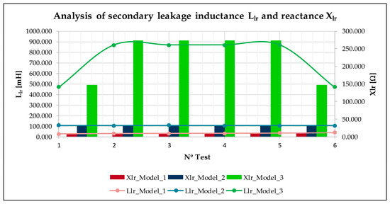
Figure 14. Secondary leakage inductance and reactance obtained in each TFLIM model.

Table 8. Values related to specific gain Λ_Llr.

Llr (mH)
Nº Test	TFLIM Models			Variation (%)		Gain: ΛLlr (mH/N)
	Model 1	Model 2	Model 3	∆ Llr2−1	∆ Llr3−2	ΛLlr2−1	ΛLlr3−2
Test 1	24.700	106.300	470.200	76.764	77.393	4.148	13.845
Test 2	28.300	104.600	868.000	72.945	87.949	3.878	29.044
Test 3	29.700	105.900	868.000	71.955	87.800	3.873	28.995
Test 4	31.100	104.800	868.300	70.324	87.930	3.746	29.048
Test 5	32.900	105.000	868.800	68.667	87.914	3.665	29.060
Test 6	37.100	105.300	470.200	64.767	77.605	3.467	13.883

The analysis of this indicator allows us to confirm that the evolution of $L_{lr}$ is completely different from $L_{ls}$, as ${\Lambda }_{Llr}^{2-1}<{\Lambda }_{Llr}^{3-2}$. The geometric changes have a greater influence on $L_{lr}$ than on $L_{ls}$. Thus, a value of ${\Lambda }_{Llr}^{2-1}\approx 4.14 \mathrm{m}\mathrm{H}/\mathrm{N}$ is obtained in the most unfavourable case. However, for Model 3, the value of the indicator increases considerably to values close to ${\Lambda }_{Llr}^{3-2}\approx 29 \mathrm{m}\mathrm{H}/\mathrm{N}$.

6.4. Secondary Equivalent Resistance, R_r

In this section, we discuss the changes in the equivalent secondary resistance $R_r$ and the equivalent secondary impedance $Z_r$. Regarding $R_r$ plotted on the left y-axis of Figure 15, the following relationship is obtained: $R_{r\_Model\_2}<R_{r\_Model\_1}<R_{r\_Model\_3}$. In Models 1 and 2, which operate under an exclusive transverse magnetic flux (${\varphi }_{trv}$) configuration, it can be concluded that the addition of the two non-conductive slots lead to a reduction in the resistance of the secondary in Model 2. For a better understanding of this result, we use the following variables: ${R_{r\_Model\_2}}^c$ (superscript c refers to the central section located above the central tooth of the TFLIM) is the equivalent resistance corresponding to the central aluminium section and ${R_{r\_Model\_2}}^r$ and ${R_{r\_Model\_2}}^l$ corresponding to two lateral aluminium sections located to the right and left, respectively (the superscripts r and l refer to the right and left sections located above the extreme primary teeth of the TFLIM).

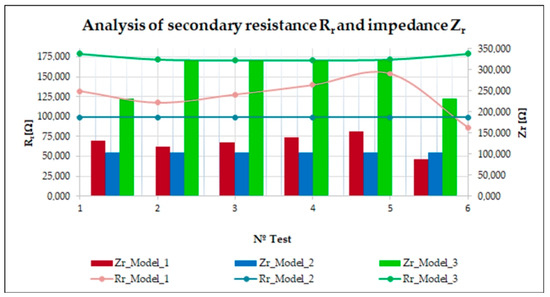
Figure 15. $R_r$ and $Z_r$ in the different TFLIM models during the tests.

Model 2 is internally configured as a triple linear motor where each of the three aluminium sections generates a positive thrust in the direction of the movement. Consequently, according to Equation (38), the three new sections of Model 2 operate in parallel, so the equivalent resistance is lower than the initial resistance of the aluminium plate in Model 1. However, when we introduce a new longitudinal flux (${\varphi }_{long}$) in Model 3, an increase in secondary resistance $∆R_r$ occurs. This result is consistent throughout the six tests conducted.

It is worth noting that throughout the tests, $R_{r\_Model\_2}$ and $R_{r\_Model\_3}$ have a consistent value over the six tests, around 100 Ω for Model 1 and 175 Ω for Model 3. Model 1 shows some variability, with the maximum value of $R_{r\_Model\_1}$ (see Figure 15) reaching a value close to 155 Ω in test number 5.

$$\underset{\begin{array}{c}{\varphi }_{trv}\\ \end{array}}{\underbrace{\underset{R_{r\_Model\_2}}{\underbrace{\left({R_{r\_Model\_2}}^r∕∕{R_{r\_Model\_2}}^l\right)∕∕{R_{r\_Model\_2}}^c}}}}<\underset{{\varphi }_{trv}}{\underbrace{R_{r\_Model\_1}}}<\underset{R_{r\_Model\_3}}{\underbrace{R_{r\_Model\_2}+\stackrel{\left({{\varphi }_{trv},\varphi }_{long}\right)}{\overbrace{∆R_r}}}}$$

(38)

A similar behaviour is obtained with the total secondary impedance, where $Z_{r\_Model\_2}<Z_{r\_Model\_1}<Z_{r\_Model\_3}$. The right y-axis of Figure 15 shows the combined action of resistance and scattering reactance associated with each model (see Equation (39)). $Z_{r\_Model\_3}$ reaches up to 350 Ω. Models 1 and 2 have values very close to the secondary resistance $R_r$, as shown in Equation (40).

$$\underset{{\varphi }_{trv}}{\underbrace{\stackrel{Z_{r\_Model\_2}}{\overbrace{\left(R_{r\_Model\_2}+j·X_{lr\_Model\_2}\right)}}<\stackrel{Z_{r\_Model\_1}}{\overbrace{\left(R_{r\_Model\_1}+j·X_{lr\_Model\_1}\right)}}}}<\stackrel{Z_{r\_Model\_3}}{\overbrace{\underset{\left({{\varphi }_{trv},\varphi }_{long}\right)}{\underbrace{\left(R_{r\_Model\_3}+j·X_{lr\_Model\_3}\right) }}}}$$

(39)

$$Z_{r\_Model\_\mathrm{1,2}}=\underset{R_{r\_Model\_\mathrm{1,2}}\gg X_{lr\_Model\_\mathrm{1,2}}}{\underbrace{\sqrt{{R_{r\_Model\_\mathrm{1,2}}}^2+{X_{lr\_Model\_\mathrm{1,2}}}^2}}}\approx R_{r_{Mode{l}_{\mathrm{1,2}}}}$$

(40)

Finally, to evaluate the result of $R_r$, the coefficient ${\Lambda }_{R_r}^{i-j}\left(\mathrm{m}\Omega /\mathrm{N}\right)$) is proposed (see Equation (41) and values in Table 9). Firstly, if we analyse the value of $\Delta R_r$, it can be observed that $\Delta R_r^{2-1}<\Delta R_r^{3-2}$. That represents an increase for Model 3 between 42.157 mΩ and 44.640 mΩ for all tests. Secondly, gains ${\Lambda }_{R_r}^{3-2}>{\Lambda }_{R_r}^{2-1}$, indicating that the model with mixed magnetic flow experiments showed a greater increase in secondary resistance for each unit of force. Thus, tests 1 and 6 return lower values, with a gain close to 3.035 mΩ/N. Model 2 in test 2 has the lowest gain value with only 0.936 mΩ/N.

$${\Lambda }_{R_r}^{i-j}={\left(\raisebox{1ex}{$\Delta R_r$}\!\left/ \!\raisebox{-1ex}{$\Delta F_y$}\right.\right)}_{i-j}$$

(41)

Table 9. Values related to specific gain Λ_Rr.

Rr (mΩ)
Nº Test	TFLIM Models			Variation (%)		Gain: ΛRr (mΩ/N)
	Model 1	Model 2	Model 3	∆ Rr2−1	∆ Rr3−2	ΛRr2−1	ΛRr3−2
Test 1	131.900	98.941	178.700	24.988	44.633	1.675	3.035
Test 2	117.300	98.893	171.800	15.692	42.437	0.936	2.774
Test 3	127.600	98.911	171.000	22.484	42.157	1.458	2.743
Test 4	139.500	98.903	171.000	29.101	42.162	2.063	2.743
Test 5	153.900	98.913	171.800	35.729	42.425	2.795	2.773
Test 6	86.300	98.928	178.700	14.632	44.640	0.642	3.035

6.5. Qualitative Analysis of Thrust Force in TFLIM According to Electric Parameters

In conclusion, it is necessary to conduct a brief qualitative analysis of the TFLIM’s behaviour, which should be explained by combining the action of three EC parameters ($X_m$, $R_r$ and $X_{lr}$) with the influence of the thrust force developed by the TFLIM. The studies carried out highlight three important trends that determine the thrust evolution without considering the dynamic longitudinal edge effect. Table 10 presents the evolutions of the three electrical parameters, including the mathematical expression of the thrust [18].

Table 10. Influence of the evolution of electrical parameters on thrust force.

Qualitative Analysis of Thrust Force in TFLIM
Trend I	${\chi }_{m\_Model\_3}>{\chi }_{m\_Model\_2}>{\chi }_{m\_Model\_1}$
Trend II	$R_{r\_Model\_2}<R_{r\_Model\_1}<R_{r\_Model\_3}$
Trend III	$Z_{r\_Model\_2}<Z_{r\_Model\_1}<Z_{r\_Model\_3}$
${\mathit{F}}_{\mathit{y}}\mathbf{=}\raisebox{1ex}{$\mathbf{3}\mathbf{·}{\left({\mathit{I}}_{\mathbf{2}}\right)}^{\mathbf{2}}\mathbf{·}{\mathit{R}}_{\mathit{r}}$}\!\left/ \!\raisebox{-1ex}{$\mathbf{2}\mathbf{·}\mathit{\pi }\mathbf{·}{\mathit{f}}_{\mathbf{1}}\mathbf{·}\mathit{s}$}\right.\mathbf{=}\raisebox{1ex}{$\mathbf{3}\mathbf{·}{\left(\raisebox{1ex}{${\mathit{E}}_{\mathbf{1}}$}\!\left/ \!\raisebox{-1ex}{$\left({\mathit{R}}_{\mathit{r}}\mathbf{+}\mathit{j}\mathbf{\cdot }{\mathit{X}}_{\mathit{l}\mathit{r}}\right)$}\right.\right)}^{\mathbf{2}}\mathbf{·}{\mathit{R}}_{\mathit{r}}$}\!\left/ \!\raisebox{-1ex}{$\mathbf{2}\mathbf{·}\mathit{\pi }\mathbf{·}{\mathit{f}}_{\mathbf{1}}\mathbf{·}\mathit{s}$}\right.\mathbf{=}\raisebox{1ex}{$\left(\mathbf{3}\mathbf{·}{\left(\raisebox{1ex}{${\mathit{I}}_{\mathit{m}}\mathbf{·}{\mathit{X}}_{\mathit{m}}$}\!\left/ \!\raisebox{-1ex}{${\mathit{Z}}_{\mathit{r}}$}\right.\right)}^{\mathbf{2}}\mathbf{·}{\mathit{R}}_{\mathit{r}}\right)$}\!\left/ \!\raisebox{-1ex}{$\mathbf{2}\mathbf{·}\mathit{\pi }\mathbf{·}{\mathit{f}}_{\mathbf{1}}\mathbf{·}\mathit{s}$}\right.$

7. Estimation of Equivalent Air Gap ${\mathit{g}}_{\mathit{s}\mathit{e}}$ and Equivalent Secondary Conductivity ${\mathit{\sigma }}_{\mathit{s}\mathit{e}}$

After we computed the EC parameters to evaluate the effect of the geometric changes, we to estimated five relevant parameters used in electrical machines. These parameters include several important electromagnetic phenomena, and all of them are dimensionless parameters. We will obtain the values of the Carter´s coefficient $K_c$, the fringing effect parameter $K_{Fr},$ the skin effect parameter $K_{skin}$, the saturation factor of the iron layer $K_{ssi}$, and the goodness factor, $G_{se}$. All parameters are explained in the next subsections, as it is shown in Figure 16 [31,32,33]. These five parameters will be used to estimate the effective air gap and the effective secondary conductivity.

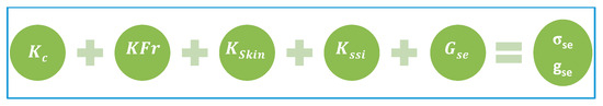
Figure 16. Schematic diagram to obtain $g_{se}$ and ${\sigma }_{se}$.

7.1. The Secondary Equivalent Air Gap $g_{se}$

Equation (42) calculates the equivalent air gap of the motor given by $g_{se}(\mathrm{m}\mathrm{m})$. This definition of air gap considers two fundamental aspects. Firstly, the magnetic air gap ($g_{mag}(\mathrm{m}\mathrm{m})$) is equivalent to the sum of the mechanical air gap ($g_{mec}(\mathrm{m}\mathrm{m})=5 \mathrm{m}\mathrm{m}$) and the thickness of the first layer of aluminium in the secondary ($h_{Al}(\mathrm{m}\mathrm{m})=10 \mathrm{m}\mathrm{m}$), which has a relative permeability value of ${\mu }_r=1$. Secondly, the path of the magnetic flux lines is increased by two phenomena quantified by the parameters $K_c$ and $K_{Fr}$.

$$g_{se}\left[mm\right]=g_{mag}·K_c·K_{Fr}=\left(\underset{g_{mag}}{\underbrace{g_{mec}+h_{Al}}}\right)·K_c·K_{Fr}$$

(42)

7.1.1. Computation of Carter´s Coefficient

Carter´s coefficient considers the effect of the air gap magnetic flux density, which varies when opening the primary slots [18]. Equations (43) and (44) calculate this coefficient, where ${\tau }_u(\mathrm{m}\mathrm{m})$ is the slot pitch, $b_1(\mathrm{m}\mathrm{m})$ is the slot opening, and $b_e (\mathrm{m}\mathrm{m})$ the equivalent slot opening [27].

$$K_c=\raisebox{1ex}{${\tau }_u$}\!\left/ \!\raisebox{-1ex}{$\left({\tau }_u-b_e\right)$}\right.=\raisebox{1ex}{${\tau }_u$}\!\left/ \!\raisebox{-1ex}{$\left({\tau }_u-k·b_1\right)$}\right.$$

(43)

$$k=\raisebox{1ex}{$2$}\!\left/ \!\raisebox{-1ex}{$\pi $}\right.·\left(arctag\left(\raisebox{1ex}{$b_1$}\!\left/ \!\raisebox{-1ex}{$2·g_{mec}$}\right.\right)-2·g_{mec}·\mathit{ln}\sqrt{1+{\left(\raisebox{1ex}{$b_1$}\!\left/ \!\raisebox{-1ex}{$2·g_{mec}$}\right.\right)}^2}\right)$$

(44)

We considered a separation depending on the topology of the magnetic flux that operates inside the TFLIM. So, for Model 1 and Model 2, which work with transversal magnetic flux, we define Carter´s coefficient with the parameter $K_{c\_trv}$. For Model 3, where there is a new longitudinal magnetic flux, it is necessary to define a new parameter to consider the slot opening along the longitudinal direction, called $K_{c\_long}.$ These parameters are defined in the following equations:

• Transverse Magnetic Flux. Equations (45) and (46) define $K_{c\_trv}$ for Models 1 and 2, where ${\tau }_{u_{trv}}(\mathrm{m}\mathrm{m}) is$ the slot pitch along the transversal direction and $b_{1\_trv} (\mathrm{m}\mathrm{m})$ and $b_{e\_trv} (\mathrm{m}\mathrm{m})$ are the slot opening and equivalent slot opening, respectively.

  $$K_{c_{trv}}=\raisebox{1ex}{${\tau }_{u_{trv}}$}\!\left/ \!\raisebox{-1ex}{$\left({\tau }_{u_{trv}}-b_{e_{trv}}\right)$}\right.=\raisebox{1ex}{${\tau }_{u_{trv}}$}\!\left/ \!\raisebox{-1ex}{$\left({\tau }_{u_{trv}}-k_{trv}·b_{1_{trv}}\right)$}\right.$$

  (45)

  $$k_{trv}=\raisebox{1ex}{$2$}\!\left/ \!\raisebox{-1ex}{$\pi $}\right.·\left(arctag\left(\raisebox{1ex}{$b_{1_{trv}}$}\!\left/ \!\raisebox{-1ex}{$2·g_{mec}$}\right.\right)-2·g_{mec}·\mathit{ln}\sqrt{1+{\left(\raisebox{1ex}{$b_{1_{trv}}$}\!\left/ \!\raisebox{-1ex}{$2·g_{mec}$}\right.\right)}^2}\right)$$

  (46)
• Longitudinal Magnetic Flux. Equations (47) and (48) calculate $K_{c\_long}$ for Model 3, where ${\tau }_{u\_long}(\mathrm{m}\mathrm{m}) \mathrm{i}\mathrm{s}$ the slot pitch along the longitudinal direction and $b_{1\_long}(\mathrm{m}\mathrm{m})$ and $b_{e\_long}(\mathrm{m}\mathrm{m})$ are the slot opening and the equivalent slot opening, respectively. In Model 3, transverse and longitudinal fluxes work simultaneously; therefore, we must define a Carter´s coefficient that considers both opening slots, called $K_{c\_mix}$ (see Equation (49)). Therefore, the mean value between the transverse Carter´s coefficient and longitudinal Carter´s coefficient is computed [9].

  $$K_{c\_long}=\raisebox{1ex}{${\tau }_{u\_long}$}\!\left/ \!\raisebox{-1ex}{$\left({\tau }_{u\_long}-b_{e\_long}\right)$}\right.=\raisebox{1ex}{${\tau }_{u_{long}}$}\!\left/ \!\raisebox{-1ex}{$\left({\tau }_{u\_long}-k_{long}·b_1\right)$}\right.$$

  (47)

  $$k_{long}=\raisebox{1ex}{$2$}\!\left/ \!\raisebox{-1ex}{$\pi $}\right.·\left(arctag\left(\raisebox{1ex}{$b_{1\_long}$}\!\left/ \!\raisebox{-1ex}{$2·g_{mec}$}\right.\right)-2·g_{mec}·\mathit{ln}\sqrt{1+{\left(\raisebox{1ex}{$b_{1\_long}$}\!\left/ \!\raisebox{-1ex}{$2·g_{mec}$}\right.\right)}^2}\right)$$

  (48)

  $$K_{c\_mix}=\raisebox{1ex}{$\left(K_{c_{trv}}+K_{c_{long}}\right)$}\!\left/ \!\raisebox{-1ex}{$2$}\right.$$

  (49)

All calculated $K_c$ parameters are shown at the end of this section, and the main conclusions are as follows:

• Model 1 and Model 2, which operate only with transverse magnetic flux, present the same slot pitch ${\tau }_{\mathrm{u}\_\mathrm{t}\mathrm{r}\mathrm{v}}=72.5 \mathrm{m}\mathrm{m},$ and its opening slot effect is similar in both cases. So, we obtain a value of ${\mathrm{K}}_{\mathrm{c}\_\mathrm{t}\mathrm{r}\mathrm{v}}=1.648$ that implies an equivalent slot opening around ${\mathrm{b}}_{\mathrm{e}\_\mathrm{l}\mathrm{o}\mathrm{n}\mathrm{g}}=3.8 \mathrm{m}\mathrm{m}$. So, in TFLIM, the effect of slot opening is higher than in LFLIM. ${\mathrm{K}}_{\mathrm{c}\_\mathrm{T}\mathrm{F}\mathrm{L}\mathrm{I}\mathrm{M}}>{\mathrm{K}}_{\mathrm{c}\_\mathrm{L}\mathrm{F}\mathrm{L}\mathrm{I}\mathrm{M}}$ and oscillates between 1.1 and 1.3 approximately [18].
• However, by adding a new longitudinal magnetic flux in Model 3, the Carter coefficient is also modified because the longitudinal magnetic circuit has a new slot pith attached ${\tau }_{\mathrm{u}\_\mathrm{l}\mathrm{o}\mathrm{n}\mathrm{g}}=16.5 \mathrm{m}\mathrm{m}$. It is necessary to evaluate the slot opening effect. The value of ${\tau }_{\mathrm{u}\_\mathrm{l}\mathrm{o}\mathrm{n}\mathrm{g}}.$ implies a new ${\mathrm{K}}_{\mathrm{c}\_\mathrm{l}\mathrm{o}\mathrm{n}\mathrm{g}}=1.299$ with an equivalent slot opening of ${\mathrm{b}}_{\mathrm{e}\_\mathrm{l}\mathrm{o}\mathrm{n}\mathrm{g}}=$ 3.8 mm. Consequently, we obtain a relationship between both Carter´s coefficients, where ${\mathrm{K}}_{\mathrm{c}\_\mathrm{t}\mathrm{r}\mathrm{v}}>{\mathrm{K}}_{\mathrm{c}\_\mathrm{l}\mathrm{o}\mathrm{n}\mathrm{g}}$. Furthermore, the presence of both magnetic fluxes configures the equivalent magnetic circuit with a new equivalent slot opening, whose influence we estimate with ${\mathrm{K}}_{\mathrm{c}\_\mathrm{m}\mathrm{i}\mathrm{x}}=1.4736.$ So, we can determine that ${\mathrm{K}}_{\mathrm{c}\_\mathrm{t}\mathrm{r}\mathrm{v}}>{\mathrm{K}}_{\mathrm{c}\_\mathrm{m}\mathrm{i}\mathrm{x}}>{\mathrm{K}}_{\mathrm{c}\_\mathrm{l}\mathrm{o}\mathrm{n}\mathrm{g}}$. This result is very relevant because we can quantify the influence of adding a new configuration into the primary part with a central ferromagnetic yoke.

7.1.2. Computation of Fringing Coefficient, ${\mathrm{K}}_{\mathrm{F}\mathrm{r}}$

$K_{Fr}$ quantifies the fringing effect along the air gap. It is calculated using Equation (50), where its value is equal to one ($K_{Fr}=1$) for all TFLIM models.

$$K_{Fr}\approx \raisebox{1ex}{$\mathit{sinh}\left(\frac{g_{mec}}{{2·\tau }_p}\right)$}\!\left/ \!\raisebox{-1ex}{$\left(\frac{g_{mec}}{{2·\tau }_p}\right)$}\right.\approx 1$$

(50)

7.1.3. Secondary Equivalent Air Gap

To better show the effect of the equivalent air gap for all models, we define the coefficient $r_{g_{se}}\left(\mathrm{\%}\right)$ that compares both air gaps, $g_{mag}$ and $g_{se}$. The results obtained from Equation (51) are shown in Table 11. Observe that $\left(r_{g_{se}\_Model\_1}=r_{g_{se}\_Model\_2}\right)<r_{g_{se}\_Model\_3}$. Using the Carter coefficient, we can conclude that Model 1 and Model 2 have the same value of $g_{se}=24.722 \mathrm{m}\mathrm{m}$ and $r_{g_{se}}=60.67\mathrm{\%}$. Model 3 reduces the effective air gap value to around 22.1 mm, and consequently, the value of $r_{g_{se}}$ increases by 7 percentage points compared to the previous models.

$$r_{g_{se}}\left[\mathrm{\%}\right]=\left(\raisebox{1ex}{$g_{mag}$}\!\left/ \!\raisebox{-1ex}{$g_{se}$}\right.\right)·100$$

(51)

Table 11. Values of g_se and r_gse obtained for each TFLIM model.

Values of Secondary Equivalent Air Gap, gse (mm)
gmag (mm) = 15	TFLIM_Model 1	TFLIM_Model 2	TFLIM_Model 3
gse (mm)	24.722	24.722	22.103
rgse (%)	60.67	60.67	67.86

7.2. The Equivalent Secondary Conductivity ${\sigma }_{se}(S/m)$

In this section, we calculate the equivalent of secondary conductivity ${\sigma }_{se}$ [18]. In the following subsections, we describe the successive steps necessary to obtain this coefficient for the three proposed TFLIM models. Section 7.2.1 describes the calculation of the magnetic saturation effect. Section 7.2.2 presents the high influence of the skin effect. Section 7.2.3 shows how to obtain the goodness factor, and Section 7.2.4 includes the computation of the effect of transverse edge in the different topologies. Finally, in Section 7.2.5, we calculate ${\sigma }_{se}$.

7.2.1. Computation of Saturation Coefficient ${\mathrm{K}}_{\mathrm{s}\mathrm{s}\mathrm{i}}$

To compute the dimensionless parameter $K_{ssi}$, we use the Equations (52) and (53), where ${\delta }_{iron} (\mathrm{m}\mathrm{m})$ is the depth of the ac field penetration inside the ferromagnetic layer and ${\mu }_{iron}=2500$ the relative permeability of the iron layer. In Equation (53), $B_t^{iron} (T)$ is the tangential component of the magnetic flux density on the back-iron upper surface, $f_1 (\mathrm{H}\mathrm{z})=50$ is the nominal frequency and ${\sigma }_{iron} (\mathrm{S}/\mathrm{m})$ is the electric conductivity of the iron layer. Particularly, we use ${\sigma }_{iron}=0 \raisebox{1ex}{$\mathrm{S}$}\!\left/ \!\raisebox{-1ex}{$\mathrm{m}\mathrm{m}$}\right.$.

$$K_{ssi}=\raisebox{1ex}{$\left(2·{\tau }_p^2·{\mu }_0\right)$}\!\left/ \!\raisebox{-1ex}{$\left(2·{\pi }^2·\left(g_{mec}+h_{Al}\right)·{\delta }_{iron}·{\mu }_{iron}\right)$}\right.\approx \raisebox{1ex}{$\left(2·{\tau }_p^2·{\mu }_0\right)$}\!\left/ \!\raisebox{-1ex}{$\left(2·{\pi }^2·\left(g_{mec}+h_{Al}\right)·\left(\raisebox{1ex}{$1$}\!\left/ \!\raisebox{-1ex}{$\left(\raisebox{1ex}{$\pi $}\!\left/ \!\raisebox{-1ex}{${\tau }_p$}\right.\right)$}\right.\right)·{\mu }_{iron}\right)$}\right.$$

(52)

$${\delta }_{iron}=Re\left[\raisebox{1ex}{$1$}\!\left/ \!\raisebox{-1ex}{$\sqrt{{\left(\raisebox{1ex}{$\pi $}\!\left/ \!\raisebox{-1ex}{${\tau }_p$}\right.\right)}^2+j·s·f_1·2·\pi ·{\mu }_0·{\mu }_{iron}·B_t^{iron}·{\sigma }_{iron}}$}\right.\right]\approx \raisebox{1ex}{$1$}\!\left/ \!\raisebox{-1ex}{$\left(\raisebox{1ex}{$\pi $}\!\left/ \!\raisebox{-1ex}{${\tau }_p$}\right.\right)$}\right.$$

(53)

7.2.2. Computation of Skin Effect Coefficient ${\mathrm{K}}_{\mathrm{s}\mathrm{k}\mathrm{i}\mathrm{n}}$

In this section, it is estimated the skin effect phenomenon that appears when there is an alternating current in a conductor that produces an alternating flux inside the armature. This effect increments the DC resistance of the conductor material. To calculate it, we define the following parameters (see Equations (54)–(58)):

• Computation of $\mathsf{\alpha }$: It is the propagation coefficient used in Equation (54), where ${\mu }_0=4·\pi ·{10}^{-7}\raisebox{1ex}{$\mathrm{H}$}\!\left/ \!\raisebox{-1ex}{$\mathrm{m}$}\right.$ is the magnetic permeability of free space ${\mu }_0$, ${\sigma }_{copper}=4.21·{10}^7 \mathrm{S}·{\mathrm{m}}^{-1}$ is the copper conductivity, and ${\omega }_e(\mathrm{r}\mathrm{a}\mathrm{d}/\mathrm{s})$ is the source electrical angular frequency. $\mathrm{f}(\mathrm{H}\mathrm{z})$ is fixed to 50 Hz, and ${\rho }_{penetration}(\mathrm{m})$ is the penetration depth.

  $$\alpha =\sqrt{\raisebox{1ex}{${\mu }_0·{\sigma }_{copper}·{\omega }_e$}\!\left/ \!\raisebox{-1ex}{$2$}\right.}=\raisebox{1ex}{$1$}\!\left/ \!\raisebox{-1ex}{${\rho }_{penetration}$}\right.$$

  (54)
• Estimation of $\xi$: This coefficient can be defined using a dimensionless number (see Equation (55)), where ${ h}_{slot} (\mathrm{m})$ is the height of the slot.

  $$\xi =\alpha ·h_{slot}$$

  (55)
• Computation of $K_{Rac}$: Equation (56) defines the dimensionless parameter $K_{Rac}$, which modifies the initial value of $R_{s\_dc}$. This was explained before, and it is the DC value of the resistance per phase. $R_{s\_ac}$ corresponds to the value of the alternating current resistance for a single-layer winding.

  $$\begin{gathered} R_{s_{ac}}=R_{s_{dc}}·K_{Rac}= \\ \underset{R_{s_{dc}}}{\left(\underbrace{\raisebox{1ex}{$n_{phase}·\left({\rho }_{Cu}·{\overline{L}}_{coil}·N_{phase}\right) $}\!\left/ \!\raisebox{-1ex}{$A_c$}\right.}\right)}·\underset{K_{Rac}\ge 1}{\underbrace{\xi \left(·\raisebox{1ex}{$\mathit{sinh}\left(2·\xi \right)+\mathit{sin}\left(2·\xi \right)$}\!\left/ \!\raisebox{-1ex}{$\mathit{cosh}\left(2·\xi \right)-\mathit{cos}\left(2·\xi \right)$}\right.\right)} } \end{gathered}$$

  (56)
• Computation of $K_{Rmac}$: Using Equation (57), with the dimensionless parameters $K_{Rmac}$, we can correct the skin effect. The AC resistance value is adapted to windings with layers not equal to 1. Variable $m$ is the number of layers of a double-layer windings configuration, where $m$ is equal to 2.

  $$\begin{gathered} K_{Skin}=K_{Rac}+\left(\raisebox{1ex}{$\left(m^2-1\right)$}\!\left/ \!\raisebox{-1ex}{$3$}\right.\right)·{\Psi }^{\prime }\left(\xi \right)= \\ {K}_{Rac}+\left(\raisebox{1ex}{$\left(m^2-1\right)$}\!\left/ \!\raisebox{-1ex}{$3$}\right.\right)·\left(\raisebox{1ex}{$\mathit{sinh}\left(\xi \right)+\mathit{sin}\left(\xi \right)$}\!\left/ \!\raisebox{-1ex}{$\left(\left(\mathit{cosh}\left(\xi \right)+\mathit{cos}\left(\xi \right)\right)·\xi \right)$}\right.\right) \end{gathered}$$

  (57)
• Estimation of equivalent resistance for alternating current: Equation (58) estimates the primary resistance of a primary winding operating under alternating current and adapted to the number of layers.

  $$R_{s\_ac}=R_{s\_dc}·K_{Skin}$$

  (58)

Table 12 shows relevant information about the skin effect phenomenon. Its design implies open slots, and therefore, the primary resistance is incremented considerably with respect to the DC value. In our work, there is a double-layer winding; therefore, the coefficient $K_{Rmac}$ reaches a value around 4.2, and the resistance per phase increases until 11 Ω.

Table 12. Skin effect parameters in a double-layer TFLIM.

Skin Effect Parameters
${\mathit{\rho }}_{\mathit{p}\mathit{e}\mathit{n}\mathit{e}\mathit{t}\mathit{r}\mathit{a}\mathit{t}\mathit{i}\mathit{o}\mathit{n}}(\mathbf{m})$	$\mathit{\xi }$	${\mathit{K}}_{\mathit{R}\mathit{a}\mathit{c}}$	${\mathit{K}}_{\mathit{R}\mathit{m}\mathit{a}\mathit{c}}$	${\mathit{R}}_{\mathit{s}\_\mathit{d}\mathit{c}}$ (Ω)	${\mathit{R}}_{\mathit{s}\_\mathit{a}\mathit{c}}$ (Ω)
0.01095	4.0155	4.0176	4.2654	2.58	11.0046

7.2.3. Computation of Goodness Factor, ${\mathrm{G}}_{\mathrm{s}\mathrm{e}}$

In this subsection, we compute this quotient with Equation (59), where $X_m (\Omega )$ is the magnetizing inductance and $R_r(\Omega )$ is the secondary resistance [33]. Both parameters were computed using the system of equations analysed. A good design of an LIM must use a $G_{se}$ > 1. We define $G_{se\_Model\_1}$ to determine the goodness factor for Model 1 and $G_{se\_Model\_2}$ and $G_{se\_Model\_3}$ for Model 2 and Model 3, respectively.

$$G_{se}=\raisebox{1ex}{$X_m$}\!\left/ \!\raisebox{-1ex}{$R_r$}\right.=\raisebox{1ex}{${\omega }_1·L_m$}\!\left/ \!\raisebox{-1ex}{$R_r$}\right.>1$$

(59)

From this estimation, we can conclude the following:

• Transverse Magnetic Flux: $G_{se\_Model\_1}<G_{se\_Model\_2}$. We obtain an improvement of $G_{se}$ when the TFLIM operates under transverse magnetic flux configuration. So, for Model 1, $G_{se}$ varies between 25.1 (Test 1) and 54.38 (Test 6). For Model 2, $G_{se}$ reaches a value of around 66.89 and 69.17, respectively.
• Mixed Magnetic Flux: We obtain values of $G_{se}$ for Model 3 that oscillates between values in Models 1 and 2. So, $G_{se\_Model\_1}<G_{se\_Model\_3}{<G}_{se\_Model\_2}$. The addition of a new longitudinal magnetic flux only supposes the increase in $G_{se}$ with respect to Model 1. In Test 1, the value of $G_{se}$ is around 45.9 and in Test 5 reaches a value of 51.6.

7.2.4. Computation of Transversal Coefficient ${\mathrm{K}}_{\mathrm{t}\mathrm{r}}$

After we estimated the goodness factor, we were able to compute the effective transverse edge effect $K_{trAl}$ that represents the transverse edge effect that occurs inside the aluminium layer [18]. We compare this effect between the TFLIM models that will involve a reduction in the aluminium electrical conductivity. Now, we computed all parameters of Equation (60) and $K_{trAl}$ is estimated by Equation (61).

$$G_{se}=\raisebox{1ex}{${\mu }_0·{\tau }_p^2·{\omega }_1·{\sigma }_{Al}·h_{Al}$}\!\left/ \!\raisebox{-1ex}{$\pi ·{g_{mag}·K}_{Skin}·K_c·K_{Fr}·K_{trAl}$}\right.$$

(60)

$$K_{trAl}=\raisebox{1ex}{${\mu }_0·{\tau }_p^2·{\omega }_1·{\sigma }_{Al}·h_{Al}$}\!\left/ \!\raisebox{-1ex}{$\pi ·{g_{mag}·K}_{Skin}·K_c·K_{Fr}·G_{se}$}\right.$$

(61)

7.2.5. Secondary Equivalent Conductivity

Finally, Equation (62) defines the value of the conductivity using ${\sigma }_{Al}$ that corresponds to the value of the electrical conductivity of the aluminium layer of the secondary and the electrical conductivity of the second layer of the secondary ${\sigma }_{iron}=0 \mathrm{S}/\mathrm{m}$ to minimize the computational effort (see Table 1).

$${\sigma }_{se}\left[\raisebox{1ex}{$S$}\!\left/ \!\raisebox{-1ex}{$m$}\right.\right]=\left(\raisebox{1ex}{${\sigma }_{Al}$}\!\left/ \!\raisebox{-1ex}{$K_{trAl·}{K}_{skin}$}\right.\right)·\underset{{\sigma }_{iron}=0\raisebox{1ex}{$S$}\!\left/ \!\raisebox{-1ex}{$m$}\right.}{\underbrace{\left(1+\raisebox{1ex}{${{\sigma }_{iron}·\delta }_i·K_{trAl}·K_{Skin}$}\!\left/ \!\raisebox{-1ex}{$K_{trAl}·h_{Al}$}\right.\right)}}\approx \raisebox{1ex}{${\sigma }_{Al}$}\!\left/ \!\raisebox{-1ex}{$K_{trAl·}{K}_{skin}$}\right.$$

(62)

A new ratio $r_{{\sigma }_{se}}\left(\%\right)$ is also defined by Equation (63) to assess the divergence between the electrical conductivities,${\sigma }_{Al}$ and ${\sigma }_{se}$, in percentage terms.

$$r_{{\sigma }_{se}}=\left(\raisebox{1ex}{${\sigma }_{se}$}\!\left/ \!\raisebox{-1ex}{${\sigma }_{Al}$}\right.\right)·100$$

(63)

$r_{{\sigma }_{se}}(\%)$ values are shown in Table 13. There, we can observe that ${\sigma }_{se\_Model\_3}>{\sigma }_{se\_Model\_2}>{\sigma }_{se\_Model\_1}$. This is very important and indicates that Model 2 decreases the transverse edge effect and increases in equivalent conductivity. The same occurs in Model 3, which achieves values closer to the conductivity of the aluminium plate, ${\sigma }_{Al}=3.73·{10}^7 \mathrm{S}/\mathrm{m}$. When we analyse the deviation rate between both magnitudes, we obtain that $r_{{\sigma }_{se}\_Model\_3}>r_{{\sigma }_{se}\_Model\_2}>r_{{\sigma }_{se}\_Model\_1}$. This is coherent with the previous result in Model 3, where these values increase by 20% with respect to the original conductivity. Table 14 and Table 15 show values of the parameters and variables that were calculated throughout this section.

Table 13. Values of σ_se y r_σse obtained for each TFLIM model.

Values of Secondary Equivalent Conductivity, σse (S/m)
TFLIM_Model_1
σse_Model_1 (S/m)	4.12 × 106	4.97 × 106	4.75 × 106	4.53 × 106	4.32 × 106	8.92 × 106
rσse_Model_1 (%)	11.03	13.32	12.74	12.14	11.59	23.90
TFLIM_Model_2
σse_Model_2 (S/m)	5.90 × 106	6.63 × 106	6.66 × 106	6.66 × 106	6.65 × 106	5.90 × 106
rσse_Model_2 (%)	15.83	17.78	17.85	17.87	17.82	15.83
TFLIM_Model_3
σse_Model_3 (S/m)	6.73 × 106	7.56 × 106	7.59 × 106	7.59 × 106	7.57 × 106	6.73 × 106
rσse_Model_3 (%)	18.04	20.26	20.34	20.36	20.30	18.04

Table 14. Analysis parameters of TFLIM operating with transverse magnetic flux.

TRANSVERSE MAGNETIC FLUX
Model_1						Model_2
τu_trv (mm)	b1_trv (mm)	ktrv	be_trv (mm)	gmec (mm)	gmag (mm)	τu_trv (mm)	b1_trv (mm)	ktrv	be_trv (mm)	gmec (mm)	gmag (mm)
72.5	35	0.8146	0.0038	5	10	72.5	35	0.8146	0.0038	5	10
Carter´s Coefficient Kc_trv					1.648	Carter´s Coefficient Kc_trv					1.648
Fringing Effect Coefficient KFr					1	Fringing Effect Coefficient KFr					1
Equivalent air gap get (mm)					24.722	Equivalent air gap get (mm)					24.722
Skin effect Coefficient Kskin					4.265	Skin effect Coefficient Kskin					4.265
Saturation Coefficient into Iron layer Kssi					1.29 × 10-9	Saturation Coefficient into Iron layer Kssi					1.29 × 10-9
Goodness Factor Gse						Goodness Factor Gse
Test 1	Test 2	Test 3	Test 4	Test 5	Test 6	Test 1	Test 2	Test 3	Test 4	Test 5	Test 6
25.1	30.31	28.98	27.63	26.37	54.38	66.896	68.295	65.700	68.543	68.793	69.170
Transversal edge effect Coefficient into Aluminium layer KtrAl						Transversal edge effect Coefficient into Aluminium layer KtrAl
2.125	1.760	1.841	1.931	2.023	0.981	0.797	0.781	0.812	0.778	0.775	0.771
Equivalent secondary conductivity σse (S/m)						Equivalent secondary conductivity σse (S/m)
4.12 × 106	4.97 × 106	4.75 × 106	4.53 × 106	4.32 × 106	8.92 × 106	5.9 × 106	6.63 × 106	6.66 × 106	6.66 × 106	6.65 × 106	5.90 × 106

Table 15. Analysis parameters of TFLIM operating with mixed magnetic flux.

MIXED MAGNETIC FLUX
Model 3
Transverse Magnetic Flux Parameters						Longitudinal Magnetic Flux Parameters
τu_trv (mm)	b1_trv (mm)	ktrv	be_trv (mm)	gmec (mm)	gmag (mm)	τu_long (mm)	b1_long (mm)	klong	be_long (mm)	gmec (mm)	gmag (mm)
72.5	35	0.8146	0.0285	5	10	16.5	8.5	0.4468	0.0038	5	10
Carter´s Coefficient Kc_trv					1.648	Carter´s Coefficient Kc_long					1.299
Fringing Effect Coefficient KFr					1	Fringing Effect Coefficient KFr					1
Skin effect Coefficient Kskin					4.265	Skin effect Coefficient Kskin					4.265
Mixed Magnetic Flux Parameters
Test 1	Test 2	Test 3	Test 4	Test 5	Test 6	Carter´s Coefficient Kc_mix
Goodness Factor Gse
45.907	51.557	51.761	51.810	51.668	45.907	1.4736
Transversal effect Coefficient into Aluminium layer KtrAl						Equivalent air gap get (mm)
1.300	1.157	1.153	1.152	1.155	1.2996	22.10
Equivalent secondary conductivity σse (S/m)						Saturation Coefficient into Iron layer Kssi
6.73 × 106	7.56 × 106	7.59 × 106	7.59 × 106	7.57 × 106	6.73 × 106	1.45 × 10-9

8. Conclusions

In this section, we summarize the main conclusions of the paper, emphasizing key points that are considered particularly relevant when the primary parameters of the EC using FEM-3D are obtained.

The dynamic curve of thrust force versus slip was obtained to identify speed ranges where the geometric changes introduced in the different TFLIM models are particularly significant. For the experiences, we can conclude that for slips between one ($v_{sec}=0 \mathrm{m}/\mathrm{s}$) and 0.6 ($v_{sec}=8 \mathrm{m}/\mathrm{s}$), the relationship between the thrust forces is ${\overrightarrow{F}}_{y\_Model\_3}>{\overrightarrow{F}}_{y\_Model\_2}>{\overrightarrow{F}}_{y\_Model\_1}$. We must remark that in secondary standstill conditions, the thrust force increases from Model 1 to Model 3 by around 60% and $I_{1\_Model\_1}>I_{1\_Model\_2}>I_{1\_Model\_3}$. This is a good result because we obtain an increase in the force with a lower power consumption during motor starting with Model 3.

For each of the three models, tests under conditions of secondary blocked and TFLIM operation without load, known as indirect tests, were replicated using FEM-3D. In this way, values corresponding to the variables $R_{eq}$, $L_{eq}$, and $L_s$ were obtained. The tests with secondary blocked determine that $R_{eq\_Model\_1}\le R_{eq\_Model\_2}\le R_{eq\_Model\_3}$ and $L_{eq\_Model\_1}<L_{eq\_Model\_2}<L_{eq\_Model\_3}$. Subsequently, after simulating the tests of TFLIM without load, $L_s$ has the following performance $L_{s\_Model\_3}>L_{s\_Model\_2}>L_{s\_Model\_1}$.

In our paper, a system of equations was proposed whose solution corresponds to the main parameters of the equivalent circuit ($L_m$, $L_{ls},$ $L_{lr}$ and $R_r)$. Additionally, two main currents of the machine, $I_m$ and $I_2$, will be obtained. It is important to remark that the current through the primary winding, $I_1$, is obtained with the finite element simulation tool. Regarding the magnetization inductance, we obtain that $L_{m\_Model\_3}>L_{m\_Model\_2}>L_{m\_Model\_1}$. Analyzing the behaviour of the primary and secondary leakage inductances ($L_{ls} and L_{lr}$), we establish that $L_{ls\_Model\_1}>L_{ls\_Model\_2}>L_{ls\_Model\_3}$ and $L_{lr\_Model\_3}>L_{lr\_Model\_2}>L_{lr\_Model\_1}$. Finally, the values of the equivalent secondary resistance are $R_{r\_Model\_2}<R_{r\_Model\_1}<R_{r\_Model\_3}$.

The main results obtained from the analysis of specific phenomena in linear motors were presented. The calculated Carter coefficient varies depending on the analysed topology: $K_{c\_trv}>K_{c\_mix}>K_{c\_long}$. Thus, for Model 3, this coefficient reaches a value of ${\mathrm{K}}_{\mathrm{c}\_\mathrm{m}\mathrm{i}\mathrm{x}}=1.4736$. This emphasizes that the results of $g_{se}$ must be considered in the analysis of TFLIM because $\left(g_{se\_Model\_1}=g_{se\_Model\_2}\right)>g_{se\_Model\_3}$. To complete our analysis, the secondary equivalent conductivity, which quantifies the transverse edge effect, was calculated, and we obtained that ${\sigma }_{se\_Model\_3}>{\sigma }_{se\_Model\_2}>{\sigma }_{se\_Model\_1}$. The inclusion of the two non-ferromagnetic slots implies a decrease in the transverse edge effect, increasing the useful surface of the aluminium plate.

In future work, we propose to calculate the LEE and its inclusion in the EC, specifically in the magnetizing branch. In this way, we would achieve the complete computation of the system model for each TFLIM. Additionally, a control strategy can be designed. To this end, once the motor plant is fully identified, the following steps are proposed. Firstly, the joint TFLIM-Inverter simulation must be analysed to detect additional parasitic harmonic fields, which modify the evolution of thrust force ripple [34]. Secondly, the best control strategy must be selected, especially focusing on Model 3, where two main magnetic fields, longitudinal and transverse, operate together [35,36,37].

References

- Liu, Z.; Long, Z.; Li, X. Maglev Trains. Key Underlying Technologies. In Springer Tracts in Mechanical Engineering; Springer: Berlin/Heidelberg, Germany, 2015; ISBN 978-3-662-45672-9. [Google Scholar]
- Ma, W.; Xi, L.; Zhang, Y.; He, Z.; Zhang, X.; Cai, Z. Design and comparison of linear induction motor and superconducting linear synchronous motor for electromagnetic launch. In Proceedings of the 2021 13th International Symposium on Linear Drives for Industry Applications (LDIA), Wuhan, China, 1–3 July 2021; pp. 1–5. [Google Scholar] [CrossRef]
- Priyadarshi, N.; Bhaskar, M.S.; Almakhles, D. Single Stage Explicit Double Diode Modelled PV Module Powered Linear Induction Motor Driven Water Pump System. In Proceedings of the 2023 IEEE IAS Global Conference on Emerging Technologies (GlobConET), London, UK, 19–21 May 2023; pp. 1–6. [Google Scholar] [CrossRef]
- Zhang, Q.; Liu, H.; Song, T.; Zhang, Z. A Novel, Improved Equivalent Circuit Model for Double-Sided Linear Induction Motor. Electronics 2021, 10, 1644. [Google Scholar] [CrossRef]
- Egeland, A.; Wedlund, C.S. Birkeland’s Electromagnetic Cannon. IEEE Trans. Plasma Sci. 2018, 46, 2154–2161. [Google Scholar] [CrossRef]
- Solomin, A.; Solomin, A.V.; Zamshina, L.L. Mathematical Modeling of Currents in Secondary Element of Linear Induction Motor with Transverse Magnetic Flux for Magnetic-Levitation Transport. In Proceedings of the 2019 International Conference on Industrial Engineering, Applications and Manufacturing (ICIEAM), Sochi, Russia, 25–29 March 2019; pp. 1–6. [Google Scholar] [CrossRef]
- Lee, J.Y.; Hong, J.P.; Chang, J.H.; Kang, D.H. Computation of inductance and static thrust of a permanent-magnet-type transverse flux linear motor. IEEE Trans. Ind. Appl. 2006, 42, 487–494. [Google Scholar] [CrossRef]
- Dominguez, J.A.; Duro, N.; Gaudioso, E. A 3-D simulation of a single-sided linear induction motor with transverse and longitudinal magnetic flux. Appl. Sci. 2020, 10, 7704. [Google Scholar]
- Dominguez, J.A.; Duro, N.; Gaudioso, E. Simulation of a Transverse Flux Linear Induction Motor to Determine an Equivalent Circuit Using 3D Finite Element. IEEE Access 2023, 11, 19690–19709. [Google Scholar] [CrossRef]
- Drabek, T.; Kapustka, P.; Lerch, T.; Skwarczyński, J. A Novel Approach to Transverse Flux Machine Construction. Energies 2021, 14, 7690. [Google Scholar] [CrossRef]
- Zhang, H.; Lang, F. Design and simulation of cylindrical linear induction motor mechanism based on finite element analyse. In Proceedings of the 2015 5th International Conference on Electric Utility Deregulation and Restructuring and Power Technologies (DRPT), Changsha, China, 26–29 November 2015; pp. 1804–1808. [Google Scholar] [CrossRef]
- Shvydkiy, E.; Kolesnichenko, I. 3D numerical simulation of the linear induction motor, considering magnetic saturation. In Proceedings of the 2018 IEEE Conference of Russian Young Researchers in Electrical and Electronic Engineering (EIConRus), Moscow and St. Petersburg, Russia, 29 January–1 February 2018; pp. 777–779. [Google Scholar] [CrossRef]
- Ly, G.; Zeng, D.; Zhou, T. An Advanced Equivalent Circuit Model for Linear Induction Motors. IEEE Trans. Ind. Electron. 2018, 65, 7495–7503. [Google Scholar] [CrossRef]
- Lu, J.; Tan, S.; Zhang, X.; Guan, X.; Ma, W.; Song, S. Performance Analysis of Linear Induction Motor of Electromagnetic Catapult. IEEE Trans. Plasma Sci. 2015, 43, 2081–2087. [Google Scholar] [CrossRef]
- Heidari, H.; Rassõlkin, A.; Razzaghi, A.; Vaimann, T.; Kallaste, A.; Andriushchenko, E.; Belahcen, A.; Lukichev, D.V. A Modified Dynamic Model of Single-Sided Linear Induction Motors Considering Longitudinal and Transversal Effects. Electronics 2021, 10, 993. [Google Scholar] [CrossRef]
- Duncan, J. Linear induction motor-equivalent-circuit-model. IET Elect. Power App. 1983, 130, 51–57. [Google Scholar] [CrossRef]
- Rivas, J.J.M. Estudio de la Interacción Magneto-Eléctrica en El Entrehierro de Los Motores Lineales de Inducción de Flujo Transversal. Aplicación Al Diseño de Un Prototipo Para Tracción Ferroviaria de Tren Monoviga. Ph.D. Thesis, Universidad Politécnica de Madrid, Madrid, Spain, 2003. [Google Scholar]
- Boldea, I. Linear Electric Machines, Drives, and MAGLEV’s Handbook; CRC Press: Boca Raton, FL, USA, 2013. [Google Scholar]
- Lipo, T.A. Introduction to AC Machine Design; IEEE Press Series on Power Engineering; Wiley: Hoboken, NJ, USA, 2017. [Google Scholar]
- Turoswski, J.; Turoswski, M. Engineering Electrodynamics. Electric Machine, Transformer and Power Equipment Design; CRC Press: Boca Raton, FL, USA, 2016. [Google Scholar]
- Jezierski, E. Transformer. In Theory; WNT: Warsaw, Poland, 1975. [Google Scholar]
- Kang, G.; Kim, J.; Nam, K. Parameter estimation of a linear induction motor with PWM inverter. In Proceedings of the IECON’01. 27th Annual Conference of the IEEE Industrial Electronics Society (Cat. No.37243), Denver, CO, USA, 29 November–2 December 2001; Volume 2, pp. 1321–1326. [Google Scholar] [CrossRef]
- Toro, N.; Gomez, Y.G.; Hoyos, F.; Sanchez, E. Parameter Estimation of Linear Induction Motor LabVolt 8228-02. In Proceedings of the Congreso Anual, Asociación de México de Control Automático, Saltillo, Mexico, 3–7 October 2011; pp. 5–7. [Google Scholar]
- Spasov, R.; Rachev, E.; Petrov, V.; Milenov, V. Determining the Equivalent Circuit Parameters of Three-Phase Induction Motor from the Manufacturer’s Technical Data. In Proceedings of the 2022 14th Electrical Engineering Faculty Conference (BulEF), Varna, Bulgaria, 14–17 September 2022; pp. 1–4. [Google Scholar] [CrossRef]
- Toman, M.; Cipin, R.; Vorel, P.; Prochazka, P. Identification of Induction Motor Parameters Considering Sensitivity Analysis of Measured Quantities. In Proceedings of the 2019 International Conference on Electrical Drives & Power Electronics (EDPE), The High Tatras, Slovakia, 24–26 September 2019; pp. 298–302. [Google Scholar] [CrossRef]
- Lu, J.; Ma, W. Investigation of Phase Unbalance Characteristics in the Linear Induction Coil Launcher. IEEE Trans. Plasma Sci. 2011, 39, 110–115. [Google Scholar] [CrossRef]
- Pyrhonen, J.; Jokinen, T.; Hrabovcova, V. Design of Rotating Electrical Machines; Wiley: Hoboken, NJ, USA, 2014; ISBN 978-1-118-58157-5. [Google Scholar]
- Bianchi, N. Electrical Machine Analysis Using Finite Elements; CRC Press Taylor & Francis: Boca Raton, FL, USA, 2005; ISBN 0849333997. [Google Scholar]
- Yamazaki, K. An efficient procedure to calculate equivalent circuit parameter of induction motor using 3-D nonlinear time-stepping finite-element method. IEEE Trans. Magn. 2002, 38, 1281–1284. [Google Scholar] [CrossRef]
- Huang, C.; Sun, Z.; Mao, Y.; Jia, G.; Zeng, R.; Ding, A.; Li, W. Parameter Calculation Method of Large Thrust Short Primary Linear Induction Motor. In Proceedings of the 2022 IEEE 5th International Electrical and Energy Conference (CIEEC), Nanjing, China, 27–29 May 2022; pp. 1956–1961. [Google Scholar] [CrossRef]
- Nasar, S.N.; Boldea, I. Linear Motion Electric Machines; Wiley-Interscience Publication: Hoboken, NJ, USA, 1976; ISBN 0471630292. [Google Scholar]
- Gieras, J.F. Linear Induction Drives; Clarendon Press: Oxford, UK; New York, NY, USA, 1994. [Google Scholar]
- Laithwaite, E.R. Induction Machines for Special Purposes; Chemical Publishing Company Inc.: New York, NY, USA, 1966; ISBN 978-0600411475. [Google Scholar]
- Palomino, G.G.; Conde, J.R. Comparative results of thrust ripple in several topologies of PMLSM. In Proceedings of the 2008 4th IET Conference on Power Electronics, Machines and Drives, York, UK, 2–4 April 2008; pp. 135–138. [Google Scholar] [CrossRef]
- Accetta, A.; Cirrincione, M.; D’Ippolito, F.; Pucci, M.; Sferlazza, A. Input–Output Feedback Linearization Control of a Linear Induction Motor Taking into Consideration Its Dynamic End-Effects and Iron Losses. IEEE Trans. Ind. Appl. 2022, 58, 3664–3673. [Google Scholar] [CrossRef]
- Accetta, A.; Cirrincione, M.; Pucci, M.; Sferlazza, A. State Space-Vector Model of Linear Induction Motors Including End-Effects and Iron Losses Part I: Theoretical Analysis. IEEE Trans. Ind. Appl. 2020, 56, 235–244. [Google Scholar] [CrossRef]
- Accetta, A.; Cirrincione, M.; Pucci, M.; Sferlazza, A. State-Space Vector Model of Linear Induction Motors Including End-Effects and Iron Losses—Part II: Model Identification and Results. IEEE Trans. Ind. Appl. 2020, 56, 245–255. [Google Scholar] [CrossRef]
Disclaimer/Publisher’s Note: The statements, opinions and data contained in all publications are solely those of the individual author(s) and contributor(s) and not of MDPI and/or the editor(s). MDPI and/or the editor(s) disclaim responsibility for any injury to people or property resulting from any ideas, methods, instructions or products referred to in the content. |
© 2024 by the authors. Licensee MDPI, Basel, Switzerland. This article is an open access article distributed under the terms and conditions of the Creative Commons Attribution (CC BY) license (https://creativecommons.org/licenses/by/4.0/).