Abstract
In this paper, we study Lipschitz stability of Caputo fractional differential equations with non-instantaneous impulses and state dependent delays. The study is based on Lyapunov functions and the Razumikhin technique. Our equations in particular include constant delays, time variable delay, distributed delay, etc. We consider the case of impulses that start abruptly at some points and their actions continue on given finite intervals. The study of Lipschitz stability by Lyapunov functions requires appropriate derivatives among fractional differential equations. A brief overview of different types of derivative known in the literature is given. Some sufficient conditions for uniform Lipschitz stability and uniform global Lipschitz stability are obtained by an application of several types of derivatives of Lyapunov functions. Examples are given to illustrate the results.
Keywords:
non-instantaneous impulses; Caputo fractional derivative; differential equations; state dependent delays; lipschitz stability AMS Subject Classifications:
34A37; 34K20; 34K37
1. Introduction
Many papers in the literature study stability of solutions of differential equations via Lyapunov functions. One type of stability, useful in real world problems, is the so-called Lipschitz stability and Dannan and Elaydi [1] introduced the notion of Lipschitz stability for ordinary differential equations. As noted in [1], this type of stability is important only for nonlinear problems since it coincides with uniform stability in linear systems. Based on theoretical results for Lipschitz stability in [1], the dynamic behavior of a spacecraft when a single magnetic torque-rod is used for achieving a pure spin condition is studied in [2]. Recently, stability properties of delay fractional differential equations without any type of impulse are considered and we refer the reader to [3] and the references therein.
In this paper, we study the Lipschitz stability for a nonlinear system of non-instantaneous impulsive fractional differential equations with state dependent delay (NIFrDDE). The impulses start abruptly at some points and their actions continue on given finite intervals. Non-instantaneous impulsive differential equations were introduced by Hernandez and O’Regan in 2013 (see, for example, [4]). The systematic description of solutions of both ordinary and Caputo fractional differential equations with non-instantaneous impulse and without delays is given in the monograph [5]. In addition, some results for non-instantaneous fractional equations without any type of delay are presented in [6,7,8]. In [9], Caputo fractional differential equations with time varying delays is considered (we note that the model had no impulses). However, in this paper, for the first time, we consider together
- Lipschitz stability;
- state dependent delays (note a special case is time varying delays); and
- models with non-instantaneous impulses.
There are two different approaches in the literature for the interpretation of the solution of fractional differential equations with impulses (for more details, see [6] and Chapter 2 of the book [5]). In the first interpretation, the lower limit of the fractional derivative is one and the same on the whole interval of study and at each point of jump we consider a boundary value problem defined by the impulsive function. In the second interpretation, the lower limit of the fractional derivative changes at each time of jump with the idea of considering an initial value problem at each jump point.
In this paper, we use the second approach to study Lipschitz stability properties of nonlinear non-instantaneous impulsive delay differential equations. The delays are bounded and depend on both the time and the state. Note several stability properties are studied in the literature for Caputo fractional differential equations (for example, see [10] (without delays), [3] (with delays and no impulses), and [11] (with multiple discrete delays without impulses)). Our study is based on Lyapunov functions and the Razumikhin technique. A brief overview in the literature of different types of derivatives of Lyapunov functions among the studied fractional differential equation is given. Several sufficient conditions for uniform Lipschitz stability and global uniform Lipschitz stability are obtained by an application of these derivatives. Some examples illustrating the results are given.
2. Notes on Fractional Calculus
We give the main definition of fractional derivatives used in the literature (see, for example, [12,13,14]). We give these definitions for scalar functions. Throughout the paper, we assume .
- -
- Riemann–Liouville (RL) fractional derivative:where denotes the Gamma function.
- -
- Caputo fractional derivativeNote that for a constant m the equality holds. However, for any given , we denote .
- -
- The Grünwald–Letnikov fractional derivative is given byand the Grünwald–Letnikov fractional Dini derivative bywhere and denotes the integer part of the fraction .
From the relation between the Caputo fractional derivative and the Grünwald–Letnikov fractional derivative using Equation (1), we define the Caputo fractional Dini derivative of a function as
i.e.,
The fractional derivatives for scalar functions could be easily generalized to the vector case by taking fractional derivatives with the same fractional order for all components.
3. Statement of the Problem and Basic Definitions
Let the positive constant r be given and the points be such that , . Let be the given initial time. Without loss of generality, we can assume .
Consider the space of all functions , which are piecewise continuous endowed with the norm where is a norm in .
The intervals are the intervals on which the fractional differential equations are given and on the intervals the impulsive conditions are given.
The Caputo fractional derivative has a memory and it depends significantly on its lower derivative. This property as well as the meaning of impulses in the differential equation lead to two basic approaches to Caputo fractional differential equations with non-instantaneous impulses:
- -
- Unchangeable lower limit of the Caputo fractional derivative: the lower limit of the fractional derivative is equal to the initial time on the whole interval of consideration.
- -
- Changeable lower limit of the Caputo fractional derivative: the lower limit of the fractional derivative is equal to the left end on the interval without impulses.
In this paper, we study the case of changeable lower limit of the Caputo fractional derivative.
Consider the initial value problem (IVP) for a nonlinear system of non-instantaneous impulsive fractional differential equations with state dependent delay (NIFrDDE) with :
where , denotes the Caputo fractional derivative with lower limit for the state , the functions ; , ; . Here, , i.e., represents the history of the state from time up to the present time t. Note that for any we let , i.e., the function determines the state-dependent delay. Note, the integer order differential equations with non-instantaneous impulses and state dependent delay are studied in [15].
Let be the space of all functions which are piecewise continuous on with points of discontinuity , the limits and exist, for any the Caputo fractional derivative exists and it is endowed with the norm where is a norm in .
Define the set .
We introduce the assumptions:
- A1.
- The function is such that for any the inclusion holds.
- A2.
- The function and for any the inequalities holds.
- A3.
- The functions .
- A4.
- The function .
- A5.
- The function for and for .
Remark 1.
Assumption A5 guarantees the existence of the zero solution of IVP for NIFrDDE (Equation (1)) with the zero initial function .
Remark 2.
Assumption A2 guarantees the delay of the argument in Equation (1).
Definition 1.
Let the conditions A1–A4 be satisfied. The function is a solution of the IVP in Equation (1) iff it satisfies the following integral-algebraic equation
Definition 2.
The functions are defined only on the intervals without impulses on which the differential equation is given.
We generalize Lipschitz stability ([1]) for ordinary differential equations to systems of Caputo fractional non-instantaneous impulsive differential equations with state dependent delay.
Definition 3.
The zero solution of NIFrDDE (Equation (1)) is said to be:
- -
- Uniformly Lipschitz stable if there exists and such that, for any for any initial time and any initial function , the inequality implies for where is a solution of Equation (1).
- -
- Globally uniformly Lipschitz stable if there exists such that, for any initial time and any initial function , the inequality implies for
Let , . Consider the following sets:
Remark 3.
The function , is from the class with . The function is from the class with for .
4. Lyapunov Functions and Their Derivatives among Nonlinear Non-Instantaneous Caputo Delay Fractional Differential Equations
One approach to study Lipschitz stability of solutions of Equation (1) is based on using Lyapunov-like functions. The first step is to define a Lyapunov function. The second step is to define its derivative among the fractional equation.
We use the class of Lyapunov-like functions, defined and used for impulsive differential equations in [16].
Definition 4.
Let be a given interval, and be a given set. We say that the function belongs to the class if
- -
- The function is continuous on and it is locally Lipschitz with respect to its second argument.
- -
- For each and , there exist finite limits
In connection with the Caputo fractional derivative, it is necessary to define in an appropriate way the derivative of Lyapunov functions among the studied equation. We give a brief overview of the derivatives of Lyapunov functions among solutions of fractional differential equations known and used in the literature. There are mainly three types of derivatives of Lyapunov functions from the class used in the literature to study stability properties of solutions of Caputo fractional differential in Equation (1):
- -
- First type: the Caputo fractional derivative of the function defined bywhere is a solution of Equation (1).
- -
- Second type: Dini fractional derivative of the Lyapunov function among Equation (1): Let and for a non-negative integer k. Then,where and for any . We note that, because of Assumption A2, the inequality holds (), i.e is well defined.The derivative of Equation (4) keeps the concept of fractional derivatives because it has a memory.
- -
- Third type: Caputo fractional Dini derivative of a Lyapunov function among Equation (1): Let the initial function be given and the function and for a non-negative integer k. Then,or its equivalenceThe derivative given by Equation (6) depends significantly on both the fractional order q and the initial data of IVP for FrDDE (Equation (1)) and it makes this type of derivative close to the idea of the Caputo fractional derivative of a function.
Remark 4.
For any initial data of the IVP for NIFrDDE (Equation (1)) and any function and any point for a non-negative integer k the relations
are satisfied.
Remark 5.
A derivative of among a system of Caputo fractional differential equations without delays was introduced by V. Lakshmikantham et al. [17] in 2009. Later, it was generalized for fractional equations with delays ([18,19,20]):
where .
This definition is a direct generalization of the well known Dini derivative among differential equations with ordinary derivatives. However, for equations with fractional derivatives, it seems strange. It does not depend on the order q of the fractional derivative nor on the initial time . The operator defined by Equation (9) has no memory, which is typical for the fractional derivative.
The derivative defined by Equation (9) is applied in [18] to study stability of fractional delay differential equations where in the proof of the main comparison result (Theorem 4.3 [18]) the derivative is incorrectly substituted by the Caputo fractional derivative (see Equations (20) and (30) in [18]). A similar situation occurs with the application of the derivative of Equation (9) in [20] for studying stability of impulsive fractional differential equations.
In the next example to simplify the calculations and to emphasize the derivatives and their properties, we consider the scalar case, i.e., .
Example 1.
(Lyapunov function depending directly on the time variable). Let where .
Case 1. Caputo fractional derivative. Let x be a solution of NIFrDDE (Equation (1)). Then, the fractional derivative
is difficult to obtain in the general case for any solution of Equation (1). In addition, the solution might not be differentiable on the intervals of impulses.
Case 2. Dini fractional derivative. Let and for a non-negative integer k. Then, applying Equation (4), we obtain
Case 2. Caputo fractional Dini derivative. Let and for a non-negative integer k. Then, we use Equation (6) and obtain
□
5. Comparison Results
Lemma 1.
[17]. Let be such that and there exists a point : and for . Then, .
We use the following comparison scalar fractional differential equation with non-instantaneous impulses:
where
We obtain some comparison results. Note some comparison results for fractional time delay differential equations are obtained in [18] by applying the derivative defined by Equation (9) and substituting it incorrectly as a Caputo fractional derivative (see Remark 5).
We introduce the following conditions:
- A6.
- The function is strictly decreasing with respect to its second argument, and for any the functions are nondecreasing with respect to their second argument.
- A7.
- The function for and for any the function for .
- A8.
- For all , the functions satisfies .
In our main results, we use the Lipschitz stability of the zero solution of the scalar comparison non-instantaneous impulsive fractional differential in Equation (10).
Example 2.
Let and . Consider the scalar non-instantaneous impulsive fractional differential equation
where .
Case 1. Suppose for all natural numbers the equality holds. Then, the solution of Equation (11) is given by
The solution of Equation (11) is uniformly Lipschitz stable with (see Figure 1 for the graph of the solutions with various initial values).
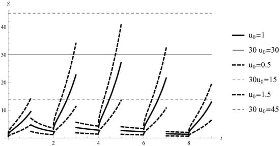
Figure 1.
Example 2. Graph of the solution of Equation (11) with for various initial values.
Case 2. Suppose for all natural numbers the equality holds. Then, the solution of Equation (11) is given by
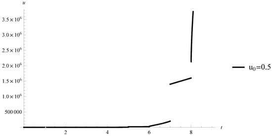
Figure 2.
Example 2. Graph of the solution of Equation (11) with .
Therefore, for the solution is Lipschitz stable but for it is not (compare with condition (A8)).
In our study, we use some comparison results. When the Caputo fractional derivative is used, then the comparison result is:
Lemma 2.
(Caputo fractional derivative). Assume the following conditions are satisfied:
- 1.
- Assumptions A1–A4 and A6 are satisfied.
- 2.
- The function is a solution of Equation (1) where , .
- 3.
- The function is such that
- (i)
- For any and for , the inequalityholds.
- (ii)
- For all the inequalityholds.
If then the inequality for holds, where is the maximal solution on of Equation (10) with .
Proof.
We use induction with respect to the intervals to prove Lemma 2. Let , . We prove
Let . Let be an arbitrary number. We prove
Note i.e., the inequality in Equation (15) holds for . If the inequality in Equation (15) is not true, then there exists a point such that .
From Lemma 1 with and the inequality holds.
From Assumption A6 and Condition 3(i), the inequality holds. The contradiction proves the validity of Equation (15). Since is an arbitrary positive number, we obtain the inequality in Equation (14) for .
Let . Then, from the impulsive equality in Equation (1), Condition 3(ii), Assumption A6 and the inequality in Equation (14) for , we obtain i.e., Equation (14) holds on .
Let . Let be an arbitrary number. We prove Equation (15) for . Note that Equation (15) is true for . If the inequality in Equation (15) is not true, then there exists a point such that .
From Lemma 1 with and , the inequality holds.
Lemma 3.
[10] Let and there exists , such that and for . Then, the inequality holds.
When the Dini fractional derivative defined by Equation (4) or Caputo fractional Dini derivative defined by Equation (5) is used then the comparison result is:
Proof.
The proof is similar to the one in Lemma 2 where instead of the Caputo fractional derivative of the Lyapunov function, we use the Dini fractional derivative or the Caputo fractional Dini derivative which are less restrictive with respect to the properties of Lyapunov functions (for example, differentiability is not required). We sketch the proof emphasizing the differences with Lemma 2.
Case 1. Let in Condition 3(i) of Lemma 4.
We use induction with respect to the intervals to prove Lemma 4. We prove the inequality in Equation (14).
Case 1.1. Let . We prove Equation (15) with an arbitrary number. Note that Equation (15) holds for . If the inequality in Equation (15) is not true, then there exists a point such that and for where . From Lemma 3 with we get the inequality
Thus
Following the proof of Lemma 3 [3] from the choice of the point , the definition of the function , the definition of the derivative , Assumption A2 and , , Assumption A6 and Condition 3(i) of Lemma 4, we obtain the inequality
with .
The inequality in Equation (17) contradicts the inequality in Equation (16). The contradiction proves the validity of Equation (15) and, therefore, the validity of Equation (14) on .
Case 1.2. Let . From the impulsive equality in Equation (1), Condition 3(ii) of Lemma 4, Assumption A6 and the inequality in Equation (14) for , we obtain for the inequalities i.e., Equation (14) holds on .
Case 1.3. Let . The proof of the inequality in Equation (15) for is similar to the one in Case 1.1 by replacing with .
Case 2. Let in Condition 3(i) of Lemma 4 be the Dini fractional derivative defined by Equation (4). Then, based on the proof in Case 1 and Remark 4, we establish Lemma 4. □
6. Main Results
Theorem 1.
(Caputo fractional derivative) Let the following conditions be satisfied:
- 1.
- Assumptions A1–A8 are fulfilled.
- 2.
- There exist a function and
- (i)
- The inequalitiesholds, where , , ;
- (ii)
- For any initial data and any solution of Equation (1) defined on such that for any , k is a non-negative integer, such that and for the inequalityholds.
- (iii)
- For any and the inequalityholds.
- 3.
- The zero solution of Equation (10) is uniformly Lipschitz stable (uniformly globally Lipschitz stable).
Then, the zero solution of Equation (1) is uniformly Lipschitz stable (uniformly globally Lipschitz stable).
Proof.
Let the zero solution of Equation (10) be uniformly Lipschitz stable. Let be an arbitrary. Without loss of generality, we assume . From Condition 3, there exist such that for any the inequality
holds, where is a solution of Equation (10) with the initial data .
From the inclusions and , there exist a function and a positive constant . Without loss of generality, we can assume . Choose the constant such that and . Therefore, .
Let . Choose the initial function such that . Therefore, , i.e., for . Consider the solution of the system in Equation (1) for the chosen initial data .
Let From the choice of and the properties of the function applying condition we get . Therefore, the function satisfies Equation (18) for with , where is a solution of Equation (10) with initial data .
Let be an arbitrary number. We prove
For , we get , i.e., the inequality in Equation (19) holds.
Assume Equation (19) is not true.
Case 1. There exists a point such that for , , i.e., for . Then, from Condition 2(i), we obtain the inequalities for , i.e., for and, according to Condition 2(ii) of Theorem 1 with , it follows that Condition 3(i) of Lemma 2 is satisfied for the solution on the interval and .
According to Lemma 2, we get
From the inequality in Equation (20) and Condition , we obtain
The contradiction proves the validity of Equation (19). From the inequality in Equation (19) and Condition 2(i), we have Theorem 1.
Case 2. There exists a point such that for , . Then, as in Case 1 we get for . Let for a natural number j. According to Condition 2(iii) of Theorem 1, we obtain . The contradiction proves this case is not possible.
Case 3. There exists a natural number k such that for and . Therefore, . The contradiction proves this case is not possible.
The proof of globally uniformly Lipschitz stability is analogous so we omit it. □
Theorem 2.
Let the conditions of Theorem 1 be satisfied where Condition 2(i) is replaced by:
the inequalities holds, where and there exists positive constant such that , for , and .
Proof.
The proof is similar to the one in Theorem 1 where .
Theorem 3.
(Dini fractional derivative/ Caputo fractional Dini derivative) Let the following conditions be satisfied:
- 1.
- Assumptions A1–A8 are fulfilled.
- 2.
- There exist a function , and
- (i)
- The inequalitiesholds, where , .
- (ii)
- (iii)
- For any and the inequalityholds.
- 3.
- The zero solution of Equation (10) is uniformly Lipschitz stable (uniformly globally Lipschitz stable).
Then, the zero solution of Equation (1) is uniformly Lipschitz stable (uniformly globally Lipschitz stable).
The proof of Theorem 3 is similar to the one in Theorem 1 where Lemma 4 is applied instead of Lemma 2.
Example 3.
Let and . Consider the non-instantaneous impulsive fractional differential equations
where , , and .
Let , .
Let be a solution of Equation (22). Let the point , k is a non-negative integer, be such that and . Using the notation and Assumption A2, it follows that and therefore or
and
Then, for all and , we get the inequality
In addition, for any natural number i, and , we get with .
According to Example 2, Case 1 and Theorem 1, the zero solution of Equation (22) is uniformly Lipschitz stable. □
Example 4.
Let and . Consider the non-instantaneous impulsive fractional differential equations
where , , , and , for .
Note that, for any , the inequality holds.
In this case, the quadratic function and Theorem 1 does not work (as it did in Example 3) because and the solution of the comparison Equation (10) with is difficult to obtain.
Consider the Lyapunov function , .
Let the function , be such that for . Let , k is a non-negative integer, be such that . From the definition of the function , it follows that for and therefore . Then
Similarly, we get .
Then, using Example 1, Case 2 and the notations , , i.e., , we get the inequality
In addition, for any natural number i, and , we get with .
According to Example 2, Case 1 and Theorem 3, the zero solution of Equation (24) is uniformly Lipschitz stable.
Author Contributions
Conceptualization, R.A., S.H. and D.O.; methodology, R.A., S.H. and D.O.; formal analysis, R.A., S.H. and D.O.
Funding
This research received no external funding.
Conflicts of Interest
The authors declare no conflict of interest.
References
- Dannan, F.M.; Elaydi, S. Lipschitz stability of nonlinear systems of differential equations. J. Math. Anal. Appl. 1986, 113, 562–577. [Google Scholar] [CrossRef]
- Zavoli, A.; Giulietti, F.; Avanzini, G.; De Matteis, G. Spacecraft dynamics under the action of Y-dot magnetic control. Acta Astronaut. 2016, 122, 146–158. [Google Scholar] [CrossRef]
- Agarwal, R.; Hristova, S.; O’Regan, D. Lyapunov Functions and Stability of Caputo Fractional Differential Equations with Delays. Differ. Equ. Dyn. Syst. 2018, 1–22. [Google Scholar] [CrossRef]
- Hernandez, E.; O’Regan, D. On a new class of abstract impulsive differential equations. Proc. Am. Math. Soc. 2013, 141, 1641–1649. [Google Scholar] [CrossRef]
- Agarwal, R.; Hristova, S.; O’Regan, D. Non-Instantaneous Impulses in Differential Equations; Springer: Berlin, Germany, 2017. [Google Scholar]
- Agarwal, R.; Hristova, S.; O’Regan, D. Non-instantaneous impulses in Caputo fractional differential equations. Fract. Calc. Appl. Anal. 2017, 20, 595–622. [Google Scholar] [CrossRef]
- Bai, L.; Nieto, J.J. Variational approach to differential equations with not instantaneous impulses. Appl. Math. Lett. 2017, 73, 44–48. [Google Scholar] [CrossRef]
- Nieto, J.J.; Uzal, J.M. Pulse positive periodic solutions for some classes of singular nonlinearities. Appl. Math. Lett. 2018, 86, 134–140. [Google Scholar] [CrossRef]
- Agarwal, R.; Hristova, S.; O’Regan, D. Lyapunov Functions to Caputo Fractional Neural Networks with Time-Varying Delays. Axioms 2018, 7, 30. [Google Scholar] [CrossRef]
- Agarwal, R.P.; O’Regan, D.; Hristova, S. Stability of Caputo fractional differential equations by Lyapunov functions. Appl. Math. 2015, 60, 653–676. [Google Scholar] [CrossRef]
- Zhang, H.; Wu, D.; Cao, J. Asymptotic Stability of Caputo Type Fractional Neutral Dynamical Systems with Multiple Discrete Delays. Abstr. Appl. Analys. 2014, 2014, 138124. [Google Scholar] [CrossRef]
- Das, S. Functional Fractional Calculus; Springer: Berlin/Heidelberg, Germany, 2011. [Google Scholar]
- Diethelm, K. The Analysis of Fractional Differential Equations; Springer: Berlin/Heidelberg, Germany, 2010. [Google Scholar]
- Podlubny, I. Fractional Differential Equations; Academic Press: San Diego, CA, USA, 1999. [Google Scholar]
- Pandey, D.N.; Das, S.; Sukavanam, N. Existence of solutions for a second order neutral differential equation with state dependent delay and not instantaneous impulses. Intern. J. Nonlinear Sci. 2014, 18, 145–155. [Google Scholar]
- Lakshmikantham, V.; Bainov, D.; Simeonov, P. Theory of Impulsive Differential Equations; World Scientific: Singapore, 1989. [Google Scholar]
- Lakshmikantham, V.; Leela, S.; Devi, J.V. Theory of Fractional Dynamic Systems; CSP: Cambridge, UK, 2009; 170p. [Google Scholar]
- Sadati, S.J.; Ghaderi, R.; Ranjbar, A. Some fractional comparison results and stability theorem for fractional time delay systems. Rom. Rep. Phy. 2013, 65, 94–102. [Google Scholar]
- Stamova, I.; Stamov, G. Lipschitz stability criteria for functional differential systems of fractional order. J. Math. Phys. 2013, 54, 043502. [Google Scholar] [CrossRef]
- Stamova, I.; Stamov, G. Functional and Impulsive Differential Equations of Fractional Order: Qualitative Analysis and Applications; CRC Press: Boca Raton, FL, USA, 2016; 276p. [Google Scholar]


© 2018 by the authors. Licensee MDPI, Basel, Switzerland. This article is an open access article distributed under the terms and conditions of the Creative Commons Attribution (CC BY) license (http://creativecommons.org/licenses/by/4.0/).