Operator Newton Method for Large-Scale Coupled Riccati Equations Arising from Jump Systems

Abstract

Consider a class of coupled discrete-time Riccati equations arising from jump systems. To compute their solutions when systems reach a steady state, we propose an operator Newton method and correspondingly establish its quadratic convergence under suitable assumptions. The advantage of the proposed method lies in the fact that its subproblems are solved using the operator Smith method, which allows it to maintain quadratic convergence in both the inner and outer iterations. Moreover, it does not require the constant term matrix of the equation to be invertible, making it more broadly applicable than existing inverse-free iterative methods. For large-scale problems, we develop a low-rank variant by incorporating truncation and compression techniques into the operator Newton framework. A complexity analysis is also provided to assess its scalability. Numerical experiments demonstrate that the presented low-rank operator Newton method is highly effective in approximating solutions to large-scale structured coupled Riccati equations.

1. Introduction

Consider a discrete-time jump control system [1,2,3], modeled by:

$$x_{k+1}=A_i{x}_k+B_i{u}_k,y_k=C_i{x}_k,i=1,\dots ,m,k=1,2,\dots ,$$

where $A_i\in {\mathbb{R}}^{N\times N}$, $B_i\in {\mathbb{R}}^{N\times m^b}$, and $C_i\in {\mathbb{R}}^{m^c\times N}$, with $m^b,m^c\ll N$. To obtain the optimal control of the above system, one has to minimize the quadratic cost function

$$J(x,u)=\sum _{k=1}^{\infty }\left[x_k^{\top }{Q}_i{x}_k+u_k^{\top }{R}_i{u}_k\right],$$

where $Q_i=C_i^{\top }{C}_i\ge 0$ and $R_i>0$ are symmetric positive semi-definite (SPSD) and symmetric positive definite (SPD) matrices, respectively, representing the state and control weighting terms in the cost function. The corresponding optimal control feedback gain is given by:

$$u_k=-{(R_i+B_i^{\top }{\mathcal{E}}_i\left(X\right)B_i)}^{-1}{B}_i^{\top }{\mathcal{E}}_i\left(X\right)A_i{x}_k,$$

where ${\mathcal{E}}_i\left(X\right)={\sum }_{j=1}^m{p}_{ij}{X}_j\in {\mathbb{R}}^{N\times N}$ is defined as a convex combination of $X_j$ via the stochastic weights $p_{ij}$. To achieve the optimal control $u_k$, one has to solve the coupled discrete-time algebraic Riccati equation (CDARE):

$${\mathcal{D}}_{Ci}\left(X\right)=-X_i+A_i^{\top }{\mathcal{E}}_i\left(X\right)A_i+Q_i-A_i^{\top }{\mathcal{E}}_i\left(X\right)B_i{\left(R_i+B_i^{\top }{\mathcal{E}}_i\left(X_i\right)B_i\right)}^{-1}{B}_i^{\top }{\mathcal{E}}_i\left(X\right)A_i=0,$$

(1)

for $i=1,\dots ,m$.

Among the various approaches developed for solving the CDARE (1), iterative methods remain prominent. Commonly used iterations typically reformulate the problem as either optimization-based methods [4] or fixed-point iterations [5,6], drawing on classical linear–quadratic regulator theory. Enhanced variants based on linear matrix inequality (LMI) formulations have also been proposed [7,8]. However, such methods often exhibit slow convergence of the objective function and limited numerical precision, particularly in large-scale or tightly coupled scenarios. Fixed-point schemes address the CDARE directly by recasting it as a fixed-point problem. Notably, Ivanov [9] introduced two distinct fixed-point iterations, which were later accelerated by incorporating extrapolation techniques that leverage information from the current iteration to replace the previous one, thereby obviously improving the convergence rate.

To circumvent the computational cost associated with explicit matrix inversion, inverse-free fixed-point methods have been introduced. These schemes are inspired by the Schulz iteration [10], which recasts matrix inversion as a Newton-type process, replacing inversions with matrix multiplications [11,12,13]. While inverse-free methods demonstrate notable computational efficiency in practice, their theoretical convergences are generally linear.

To further accelerate convergence, Newton-type methods have garnered attention. For continuous-time coupled Riccati equations, Feng and Chu [14] proposed a Newton-based approach that extends the block-diagonal structure originally developed in [15] and generalizes the pseudo-Newton strategies given in [13]. For the discrete-time case in (1), Newton-type iteration was explored in [16], though the convergence analysis therein is restricted to settings where each weighting matrix $Q_i$ is symmetric positive definite. In practical large-scale systems, however, the output matrix $C_i$ often has low rank, rendering the associated $Q_i$ only positive semi-definite. In such a case, the above Newton variants, including the inverse-free version [17], become inapplicable. For other methods applicable to similar types of equations, readers may also refer to [18,19].

The key to applying Newton’s method to large-scale CDARE (1) lies in efficiently computing the solution of large-scale coupled Stein equations (CSEs). Recently, a novel operator Smith algorithm (OSA) was introduced for solving CSEs with SPSD constant matrices [20]. This method interprets the coupling unknowns as operator-valued expressions and employs a doubling strategy to accelerate the iteration, demonstrating well-behaved numerical performance on large-scale problems. Another approach to handling large-scale CSEs with low-rank structure is to represent the low-rank matrix in the HODLR structured form [21,22]. However, after performing matrix operations with sparse matrices, the HODLR-structured matrix requires restructuring; otherwise, the dense matrix will not be adapted to large-scale computations.

Inspired by the development of OSA in [20], we propose an operator Newton method (ONM) tailored to solving large-scale CDAREs (1). The main contributions are summarized as follows:

• We develop an operator Newton iteration scheme grounded in the structure of the OSA for solving the CDARE (1) and rigorously establish the convergence as well as the convergence rate. Crucially, unlike existing inverse-free schemes [11,12,13] that require invertible $Q_i$ to initiate the iteration, our method allows for SPSD initial $Q_i$.
• A low-rank variant of the operator Newton method is constructed to address the large-scale system. When the matrix $Q_i$ admits low-rank representation, the proposed method ensures that the rank of the initial residual remains fixed across iterations, effectively mitigating rank inflation.
• We employ a doubling-based operator formulation for Newton’s subproblem, i.e., the coupled Stein equations, and embed the truncation–compression (TC) technique to control the growth of the column of low-rank factors. This enables efficient low-rank approximation to the solution without compromising numerical stability.
• We propose a scalable residual evaluation strategy for large-scale CDARE and validate the proposed method on practical problems from engineering applications. Numerical experiments demonstrate that, for a comparable level of residual accuracy, the presented operator Newton method significantly reduces CPU time relative to the standard Newton’s method with the incorporation of the HODLR structure [21,22].

The paper is structured as follows. Section 2 reviews the operator Smith algorithm, and presents several lemmas required for constructing the operator Newton method. Section 3 introduces the iterative scheme of the operator Newton method for solving the CDAREs and establishes corresponding theorems on the convergence and convergence rate. Section 4 develops a low-rank variant of the operator Newton method tailored for large-scale problems with low-rank structures. By incorporating the truncation and compression technique, the scheme effectively controls the growth of the iterative matrix sequence. A detailed analysis of the computational complexity per iteration is also provided. Section 5 demonstrates the effectiveness of the proposed operator Newton method in solving large-scale practical CDAREs.

2. Preliminaries

In this section, we begin by reviewing the iterative framework of the operator Smith algorithm (OSA), which serves as the foundation for solving the subproblems. We then establish several useful lemmas that underpin the convergence analysis of the proposed method.

2.1. Operator Smith Algorithm for Coupled Discrete-Time Stein Equations

The operator Smith algorithm [20] for solving the coupled discrete-time Stein equations

$$X_i-A_i^{\top }{\mathcal{E}}_i\left(X\right)A_i-W_i=0,i=1,\dots ,m$$

(2)

is given by the iterative scheme:

$$X_i^{(k+1)}=X_i^{\left(k\right)}+{\mathcal{F}}_i^{\left(k\right)}\left(X^{\left(k\right)}\right),X_i^{\left(0\right)}=W_i,k=0,1,2,\dots ,$$

(3)

where the operator ${\mathcal{F}}_i^{\left(k\right)}$ at the k-th iteration is defined as

$${\mathcal{F}}_i^{\left(k\right)}(·)=A_i^{\top }{\mathcal{E}}_i\left(\stackrel{2^k-1}{\overbrace{A^{\top }\mathcal{E}(\dots A^{\top }\mathcal{E}}}(·)\stackrel{2^k-1}{\overbrace{A)\dots A}}\right)A_i:=A_i^{\top }{\mathcal{E}}_i\left({\left(A^{\top }\mathcal{E}\right)}^{2^k-1}(·)A^{2^k-1}\right)A_i$$

(4)

with $A^{\top }\mathcal{E}(·)A={\sum }_{j=1}^m{A}_j^{\top }{\mathcal{E}}_i(·)A_j$ being a linear combination about j. After the k-th iteration, the expression of the iteration matrix is provided by the following theorem.

Theorem 1

([20]). Let ${\mathcal{E}}_i\left(W\right)={\sum }_{s=1}^m{p}_{i,s}{W}_s$. Then the k-th iteration $X_i^{\left(k\right)}$ produced by (3) admits the representation

$$X_i^{\left(k\right)}=W_i+A_i^{\top }{\mathcal{E}}_i\left(\sum _{j=0}^{2^k-2}{\left(A^{\top }\mathcal{E}\right)}^j\left(W\right)A^j\right)A_i,i=1,\dots ,m,$$

(5)

and the solution to (2) is given by

$$X_i^{*}=W_i+A_i^{\top }{\mathcal{E}}_i\left(\sum _{j=0}^{\infty }{\left(A^{\top }\mathcal{E}\right)}^j\left(W\right)A^j\right)A_i.$$

(6)

When each $A_i$ is d-stable, the following theorem establishes the quadratic convergence.

Theorem 2

([20]). Let $\rho :={max}_{i=1}^m\rho \left(A_i\right)$ and $p:={max}_{i,j=1}^m{p}_{ij}$ such that $mp{\rho }^m<1$. Then, for any matrix norm, the following bound holds:

$$\parallel X_i^{\left(k\right)}-X_i^{*}\parallel \le {\displaystyle \frac{{\left(mp{\rho }^m\right)}^{2^k}}{1-mp{\rho }^m}}\parallel W\parallel ,$$

where $\parallel W\parallel :={max}_{i=1}^m\parallel W_i\parallel$.

2.2. Some Lemmas

In this subsection, we introduce some lemmas which are useful for constructing the convergence of the operator Newton method.

Lemma 1.

Let $A_i$ be d-stable. Let ${\mathcal{L}}_i\left(S\right)={\sum }_{j=1}^m{c}_{ij}{S}_j$ be a linear operator with $c_{ij}>0$. Define

$$V_i=S_i-A_i^{\top }{\mathcal{L}}_i\left(S\right)A_i.$$

(7)

Then, $S_i\ge 0$ if $V_i\ge 0$ for all $i=1,\dots ,m$.

Proof. 

From (7), it follows that

$$S_i=V_i+A_i^{\top }{\mathcal{L}}_i\left(\sum _{j=0}^{\infty }{\left(A^{\top }\mathcal{L}\right)}^j\left(V\right)A^j\right)A_i.$$

Since $c_{ij}>0$ for all $i,j=1,\dots ,m$, the SPSD $V_i$ implies that $S_i\ge 0$.    □

Lemma 2.

Let A and B be SPSD matrices. If $I+AB$ is nonsingular, then

$${\parallel (I+AB)}^{-1}{\parallel }_2\le 1.$$

Proof. 

Let $y={(I+AB)}^{-1}x$ for an arbitrary nonzero vector x. Then $x=y+ABy$, and hence

$$\begin{array}{cc}\hfill {\parallel x\parallel }_2^2& =y^{\top }{(I+AB)}^{\top }(I+AB)y\hfill \\ & \ge y^{\top }y+y^{\top }(AB+BA)y+y^{\top }\left(B{A}^{2}B\right)y\hfill \\ & \ge {\parallel y\parallel }_2^2.\hfill \end{array}$$

Therefore,

$${\parallel (I+AB)}^{-1}{\parallel }_2^2=\underset{x\ne 0}{max}{\left({\displaystyle \frac{{\parallel y\parallel }_2}{{\parallel x\parallel }_2}}\right)}^2\le 1.$$

  □

Lemma 3.

The Sherman–Morrison–Woodbury formula [23] is

$${\left(A+UCV\right)}^{-1}=A^{-1}-A^{-1}U{\left(C^{-1}+V{A}^{-1}U\right)}^{-1}V{A}^{-1},$$

where $A\in {\mathbb{R}}^{n\times n}$, $U\in {\mathbb{R}}^{n\times k}$, $C\in {\mathbb{R}}^{k\times k}$, and $V\in {\mathbb{R}}^{k\times n}$ are conformable matrices.

3. Operator Newton Method

In this section, we first introduce the iterative framework of the operator Newton method (ONM) for solving the CDARE (1), and then analyze its convergence.

3.1. Iteration Format

The Fréchet derivative of the nonlinear operator ${\mathcal{D}}_{C_i}\left(X\right)$ in (1) corresponds to the linear part of the increment ${\mathcal{D}}_{C_i}(X+H)-{\mathcal{D}}_{C_i}\left(X\right)$, and is given by:

$${\mathcal{D}}_{C_i\left(X\right)}^{\prime }\left(H\right)=H_i-A_i^{\top }{(I+{\mathcal{E}}_i\left(X\right)B_i{R}_i^{-1}{B}_i^{\top })}^{-1}{\mathcal{E}}_i\left(H\right){(I+B_i{R}_i^{-1}{B}_i^{\top }{\mathcal{E}}_i\left(X\right))}^{-1}{A}_i,$$

assuming all matrix inverses exist.

Given $X_i^{\left(0\right)}$, Newton’s method based on the above derivative, can be written as

$${\mathcal{D}}_{C_i\left(X^{\left(k\right)}\right)}^{\prime }\left(X^{(k+1)}-X^{\left(k\right)}\right)=-{\mathcal{D}}_{C_i}\left(X^{\left(k\right)}\right),$$

which yields a sequence of linear subproblems of the form

$$X_i^{(k+1)}-{\left({\widehat{A}}_i^{\left(k\right)}\right)}^{\top }{\mathcal{E}}_i\left(X^{(k+1)}\right){\widehat{A}}_i^{\left(k\right)}=Q_i+L_i^{\left(k\right)}{R}_i{\left(L_i^{\left(k\right)}\right)}^{\top },i=1,\dots ,m,$$

(8)

where

$${\widehat{A}}_i^{\left(k\right)}=A_i-B_i{\left(L_i^{\left(k\right)}\right)}^{\top },L_i^{\left(k\right)}=A_i^{\top }{\mathcal{E}}_i\left(X^{\left(k\right)}\right)B_i{\left(R_i+B_i^{\top }{\mathcal{E}}_i\left(X^{\left(k\right)}\right)B_i\right)}^{-1},$$

(9)

and

$${\mathcal{E}}_i\left(X^{\left(k\right)}\right)=\sum _{s=1}^m{p}_{is}{X}_s^{\left(k\right)}.$$

Obviously, each subproblem corresponds to coupled Stein equations (8). When solved by using the OSA (3), and under some conditions specified in Theorem 3, the convergence of each inner iteration is guaranteed to be quadratic by Theorem 2. The resulting iterative scheme is referred to as the ONM.

Remark 1.

In many large-scale applications, the coefficient matrix $A_i$ ($i=1,\dots ,m$) is large and sparse with dimensions $N\times N$, while the control matrix $B_i$ is tall and skinny, meaning it has significantly fewer columns than rows. Consequently, the gain matrix $L_i^{\left(k\right)}$ computed during the ONM also exhibits a tall and skinny structure.

An advantage of the ONM emerges when the right-hand side matrix $Q_i$ in (8) admits low-rank factorization of the form $Q_i=C_i^{\top }{C}_i$, where the number of columns in $C_i$ is far less than N. In such a case, the column space of the right-hand side of (8) remains low-dimensional throughout the iteration, and the generated matrix tends to maintain a low-rank structure. This allows for efficient computation of the approximate solution with significantly reduced storage cost.

3.2. Convergence and Convergence Rate

The following theorem concludes the monotone convergence of the iteration sequence $\left\{X_i^{\left(k\right)}\right\}$ generated by ONM (8) under some mild conditions.

Theorem 3.

Let $Q_i\ge 0$, $R_i>0$ for all $i\le m$. Assume that there exists an SPD matrix ${\widehat{X}}_i$ such that ${\mathcal{D}}_{c_i}\left(\widehat{X}\right)\ge 0$ and the Euclidean norm of $A_i$ is less than one for each i. Then the sequence ${\left\{X_i^{\left(k\right)}\right\}}_{k=1}^{\infty }$ generated by (8) satisfies

1.

$X_i^{\left(k\right)}\ge X_i^{(k+1)}\ge {\widehat{X}}_i$, $k\ge 1$;

2.

$\sigma \left({\widehat{A}}_i^{\left(k\right)}\right)\in {\mathbb{D}}_{<}$, $k\ge 1$.

So there is a solution $X_i^{*}\ge 0$ to ${\mathcal{D}}_{c_i}\left(X\right)=0$ such that $\sigma \left({\widehat{A}}_i^{*}\right)\in {\mathbb{D}}_{\le }$ for each i, where

$${\widehat{A}}_i^{*}=\left(I-B_i{(R_i+B_i^{\top }{\mathcal{E}}_i\left(X^{*}\right)B_i)}^{-1}{B}_i{\mathcal{E}}_i\left(X^{*}\right)\right)A_i.$$

Proof. 

We prove items 1–2 by induction. Let $X_i^{\left(1\right)}$ be the solution of

$$X_i^{\left(1\right)}-{\left(A_i\right)}^{\top }{\mathcal{E}}_i\left(X^{\left(1\right)}\right)A_i=Q_i$$

for $i=1,\dots ,m$. As $A_i$ is d-stable and $Q_i\ge 0$, it follows from Lemma 1 that $X_i^{\left(1\right)}\ge 0$ and ${\mathcal{E}}_i\left(X^{\left(1\right)}\right)\ge 0$. Moreover, direct calculation shows that

$$\begin{array}{cc}\hfill & (X_i^{\left(1\right)}-{\widehat{X}}_i)-A_i^{\top }\left({\mathcal{E}}_i\left(X^{\left(1\right)}\right)-{\mathcal{E}}_i\left(\widehat{X}\right)\right)A_i={\mathcal{D}}_{c_i}\left(\widehat{X}\right)+{\widehat{E}}_i^{\top }{\widehat{R}}_i^{-1}{\widehat{E}}_i,\hfill \end{array}$$

where

$${\widehat{R}}_i=R_i+B_i^{\top }{\mathcal{E}}_i\left(\widehat{X}\right)B_i,{\widehat{E}}_i=B_i^{\top }{\mathcal{E}}_i\left(\widehat{X}\right)A_i.$$

Using the assumption $R_i>0$ and Lemma 1 again, one has $X_i^{\left(1\right)}\ge {\widehat{X}}_i$ for $i=1,\dots ,m$.

The SMW formula (Lemma 3) directly yields

$$\begin{array}{cc}\hfill {\widehat{A}}_i^{\left(1\right)}=& A_i-B_i{\left(L_i^{\left(1\right)}\right)}^{\top }\hfill \\ \hfill =& \left(I-B_i{(R_i+B_i^{\top }{\mathcal{E}}_i\left(X^{\left(1\right)}\right)B_i)}^{-1}{B}_i{\mathcal{E}}_i\left(X^{\left(1\right)}\right)\right)A_i\hfill \\ \hfill =& {\left(I+B_i{R}_i^{-1}{B}_i^{\top }{\mathcal{E}}_i\left(X^{\left(1\right)}\right)\right)}^{-1}{A}_i\hfill \end{array}$$

with

$${\left(L_i^{\left(1\right)}\right)}^{\top }=(R_i+B_i^{\top }{\mathcal{E}}_i\left(X^{\left(1\right)}\right)B_i{)}^{-1}{B}_i{\mathcal{E}}_i\left(X^{\left(1\right)}\right)A_i:={\left({\widehat{R}}_i^{\left(1\right)}\right)}^{-1}{B}_i{\mathcal{E}}_i\left(X^{\left(1\right)}\right)A_i.$$

It then follows Lemma 2 that

$$\rho \left({\widehat{A}}_i^{\left(1\right)}\right)\le \parallel {(I+B_i{R}_i^{-1}{B}_i^{\top }{\mathcal{E}}_i\left(X^{\left(1\right)}\right))}^{-1}{\parallel }_2{\parallel A_i\parallel }_2<1$$

(10)

for $i=1,\dots ,m$.

Now with the available $X_i^{\left(1\right)}$, ${\widehat{A}}_i^{\left(1\right)}$, and $L_i^{\left(1\right)}$, we construct sequences ${\left\{X_i^{\left(l\right)}\right\}}_{l=1}^k$, ${\left\{{\widehat{A}}_i^{\left(l\right)}\right\}}_{l=1}^k$, and ${\left\{L_i^{\left(l\right)}\right\}}_{l=1}^k$ satisfying the induction assumptions

$$X_i^{\left(1\right)}\ge \dots \ge X_i^{\left(k\right)}\ge {\widehat{X}}_i,$$

and

$$\sigma \left({\widehat{A}}_i^{\left(l\right)}\right)=\sigma \left(A_i-B_i{\left(L_i^{\left(l\right)}\right)}^{\top }\right)\subset {\mathbb{D}}_{<},$$

for $i\le m$ and $l\le k$. Here,

$${\left(L_i^{\left(l\right)}\right)}^{\top }=(R_i+B_i^{\top }{\mathcal{E}}_i\left(X^{\left(l\right)}\right)B_i{)}^{-1}{B}_i{\mathcal{E}}_i\left(X^{\left(l\right)}\right)A_i:={\left({\widehat{R}}_i^{\left(l\right)}\right)}^{-1}{B}_i{\mathcal{E}}_i\left(X^{\left(l\right)}\right)A_i.$$

(11)

We will show they are true for $k+1$.

By using Newton’s iteration, one has

$$\begin{array}{cc}\hfill & (X_i^{\left(k\right)}-X_i^{(k+1)})-{\left({\widehat{A}}_i^{\left(k\right)}\right)}^{\top }({\mathcal{E}}_i\left(X^{\left(k\right)}\right)-{\mathcal{E}}_i\left(X^{(k+1)}\right)){\widehat{A}}_i^{\left(k\right)}\hfill \\ \hfill =& (X_i^{\left(k\right)}-{\left({\widehat{A}}_i^{\left(k\right)}\right)}^{\top }{\mathcal{E}}_i\left(X^{\left(k\right)}\right){\widehat{A}}_i^{\left(k\right)})-(X_i^{(k+1)}-{\left({\widehat{A}}_i^{\left(k\right)}\right)}^{\top }{\mathcal{E}}_i\left(X^{(k+1)}\right){\widehat{A}}_i^{\left(k\right)})\hfill \\ \hfill =& (X_i^{\left(k\right)}-{\left({\widehat{A}}_i^{(k-1)}\right)}^{\top }{\mathcal{E}}_i\left(X^{\left(k\right)}\right){\widehat{A}}_i^{(k-1)})+{\left({\widehat{A}}_i^{(k-1)}\right)}^{\top }{\mathcal{E}}_i\left(X^{\left(k\right)}\right){\widehat{A}}_i^{(k-1)}-{\left({\widehat{A}}_i^{\left(k\right)}\right)}^{\top }{\mathcal{E}}_i\left(X^{\left(k\right)}\right){\widehat{A}}_i^{\left(k\right)}\hfill \\ \hfill & -L_i^{\left(k\right)}{R}_i{\left(L_i^{\left(k\right)}\right)}^{\top }-Q_i\hfill \\ \hfill =& L_i^{(k-1)}{R}_i{\left(L_i^{(k-1)}\right)}^{\top }-L_i^{\left(k\right)}{R}_i{\left(L_i^{\left(k\right)}\right)}^{\top }+{\left({\widehat{A}}_i^{(k-1)}\right)}^{\top }{\mathcal{E}}_i\left(X^{\left(k\right)}\right){\widehat{A}}_i^{(k-1)}-{\left({\widehat{A}}_i^{\left(k\right)}\right)}^{\top }{\mathcal{E}}_i\left(X^{\left(k\right)}\right){\widehat{A}}_i^{\left(k\right)}.\hfill \end{array}$$

(12)

By replacing ${\widehat{A}}_i^{(k-1)}$ and ${\widehat{A}}_i^{\left(k\right)}$ with $A_i-B_i{\left(L_i^{(k-1)}\right)}^{\top }$ and $A_i-B_i{\left(L_i^{\left(k\right)}\right)}^{\top }$, respectively, and noting $B_i^{\top }{\mathcal{E}}_i\left(X^{\left(k\right)}\right)A_i={\widehat{R}}_i^{\left(k\right)}{\left(L_i^{\left(k\right)}\right)}^{\top }$, the above expression becomes

$$\begin{array}{cc}\hfill & L_i^{(k-1)}{\widehat{R}}_i^{\left(k\right)}{\left(L_i^{(k-1)}\right)}^{\top }-L_i^{\left(k\right)}{\widehat{R}}_i^{\left(k\right)}{\left(L_i^{\left(k\right)}\right)}^{\top }\hfill \\ \hfill & -(L_i^{(k-1)}-L_i^{\left(k\right)})B_i^{\top }{\mathcal{E}}_i\left(X^{\left(k\right)}\right)A_i-A_i^{\top }{\mathcal{E}}_i\left(X^{\left(k\right)}\right)B_i{(L_i^{(k-1)}-L_i^{\left(k\right)})}^{\top }\hfill \\ \hfill =& L_i^{(k-1)}{\widehat{R}}_i^{\left(k\right)}{\left(L_i^{(k-1)}\right)}^{\top }-L_i^{\left(k\right)}{\widehat{R}}_i^{\left(k\right)}{\left(L_i^{\left(k\right)}\right)}^{\top }-(L_i^{(k-1)}-L_i^{\left(k\right)}){\widehat{R}}_i^{\left(k\right)}{\left(L_i^{\left(k\right)}\right)}^{\top }\hfill \\ \hfill & -L_i^{\left(k\right)}{\widehat{R}}_i^{\left(k\right)}{(L_i^{(k-1)}-L_i^{\left(k\right)})}^{\top }\hfill \\ \hfill =& (L_i^{(k-1)}-L_i^{\left(k\right)}){\widehat{R}}_i^{\left(k\right)}{(L_i^{(k-1)}-L_i^{\left(k\right)})}^{\top }.\hfill \end{array}$$

Since ${\widehat{A}}_i^{\left(k\right)}$ is d-stable and $(L_i^{(k-1)}-L_i^{\left(k\right)}){\widehat{R}}_i^{\left(k\right)}{(L_i^{(k-1)}-L_i^{\left(k\right)})}^{\top }\ge 0$ (as $R_i>0$), it follows from Lemma 1 that $X_i^{\left(k\right)}\ge X_i^{(k+1)}$ for $i=1,\dots ,m$.

We next show that $X_i^{(k+1)}\ge {\widehat{X}}_i$ holds for all $i\le m$. In fact, one has

$$\begin{array}{cc}\hfill & {\widehat{X}}_i-{\left({\widehat{A}}_i^{(k+1)}\right)}^{\top }{\mathcal{E}}_i\left(\widehat{X}\right){\widehat{A}}_i^{(k+1)}\hfill \\ \hfill =& {\widehat{X}}_i-{\left(A_i\right)}^{\top }{\mathcal{E}}_i\left(\widehat{X}\right)A_i+L_i^{(k+1)}{\widehat{E}}_i+{\left(L_i^{(k+1)}{\widehat{E}}_i\right)}^{\top }-L_i^{(k+1)}({\widehat{R}}_i-R_i){\left(L_i^{(k+1)}\right)}^{\top }\hfill \\ \hfill =& -{\mathcal{D}}_{c_i}\left(\widehat{X}\right)+Q_i-({\widehat{R}}_i{L}_i^{(k+1)}-{\widehat{E}}_i){\widehat{R}}_i^{-1}{({\widehat{R}}_i{L}_i^{(k+1)}-{\widehat{E}}_i)}^{\top }+L_i^{(k+1)}{R}_i{\left(L_i^{(k+1)}\right)}^{\top }.\hfill \end{array}$$

(13)

On the other hand, one can use almost the same assertion with (10) that $\rho \left({\widehat{A}}_i^{k+1}\right)<1$ for all $i\le m$. Now Newton’s iteration indicates that

$$\begin{array}{cc}\hfill & X_i^{(k+1)}-{\left({\widehat{A}}_i^{(k+1)}\right)}^{\top }{\mathcal{E}}_i\left(X^{(k+1)}\right){\widehat{A}}_i^{(k+1)}\hfill \\ \hfill =& X_i^{(k+1)}-{\left({\widehat{A}}_i^{\left(k\right)}+B_i{(L_i^{\left(k\right)}-L_i^{(k+1)})}^{\top }\right)}^{\top }{\mathcal{E}}_i\left(X^{(k+1)}\right)\left({\widehat{A}}_i^{\left(k\right)}+B_i{(L_i^{\left(k\right)}-L_i^{(k+1)})}^{\top }\right)\hfill \\ \hfill =& X_i^{(k+1)}-{\left({\widehat{A}}_i^{\left(k\right)}\right)}^{\top }{\mathcal{E}}_i\left(X^{(k+1)}\right){\widehat{A}}_i^{\left(k\right)}-{\left(B_i{(L_i^{\left(k\right)}-L_i^{(k+1)})}^{\top }\right)}^{\top }{\mathcal{E}}_i\left(X^{(k+1)}\right){\widehat{A}}_i^{\left(k\right)}\hfill \\ \hfill & -{\left({\widehat{A}}_i^{\left(k\right)}\right)}^{\top }{\mathcal{E}}_i\left(X^{(k+1)}\right)\left(B_i{(L_i^{\left(k\right)}-L_i^{(k+1)})}^{\top }\right)\hfill \\ \hfill & +{\left(B_i{(L_i^{\left(k\right)}-L_i^{(k+1)})}^{\top }\right)}^{\top }{\mathcal{E}}_i\left(X^{(k+1)}\right)\left(B_i{(L_i^{\left(k\right)}-L_i^{(k+1)})}^{\top }\right)\hfill \\ \hfill =& L_i^{\left(k\right)}{R}_i{\left(L_i^{\left(k\right)}\right)}^{\top }+Q_i-{\left(B_i{(L_i^{\left(k\right)}-L_i^{(k+1)})}^{\top }\right)}^{\top }{\mathcal{E}}_i\left(X^{(k+1)}\right)(A_i+B_i{\left(L_i^{\left(k\right)}\right)}^{\top })\hfill \\ \hfill & -{\left(A_i+B_i{\left(L_i^{\left(k\right)}\right)}^{\top }\right)}^{\top }{\mathcal{E}}_i\left(X^{(k+1)}\right)\left(B_i{(L_i^{\left(k\right)}-L_i^{(k+1)})}^{\top }\right)\hfill \\ \hfill & +{\left(B_i{(L_i^{\left(k\right)}-L_i^{(k+1)})}^{\top }\right)}^{\top }{\mathcal{E}}_i\left(X^{(k+1)}\right)\left(B_i{(L_i^{\left(k\right)}-L_i^{(k+1)})}^{\top }\right).\hfill \end{array}$$

(14)

Subtracting (13) from (14) and recollecting some terms with the equality $B_i^{\top }{\mathcal{E}}_i\left(X^{\left(k\right)}\right)A_i={\widehat{R}}_i^{\left(k\right)}{\left(L_i^{\left(k\right)}\right)}^{\top }$, one has

$$\begin{array}{cc}\hfill & X_i^{(k+1)}-{\widehat{X}}_i-{\left({\widehat{A}}_i^{(k+1)}\right)}^{\top }\left({\mathcal{E}}_i\left(X^{(k+1)}\right)-{\mathcal{E}}_i\left(\widehat{X}\right)\right){\widehat{A}}_i^{(k+1)}\hfill \\ \hfill =& {\mathcal{D}}_{c_i}\left(\widehat{X}\right)+{({\widehat{R}}_i{\left(L_i^{(k+1)}\right)}^{\top }-{\widehat{E}}_i)}^{\top }{\widehat{R}}_i^{-1}({\widehat{R}}_i{\left(L_i^{(k+1)}\right)}^{\top }-{\widehat{E}}_i)\hfill \\ \hfill & +(L_i^{(k+1)}-L_i^{\left(k\right)})(R_i+B_i^{\top }{\mathcal{E}}_i\left(X^{(k+1)}\right)B_i){(L_i^{(k+1)}-L_i^{\left(k\right)})}^{\top }.\hfill \end{array}$$

Since ${\mathcal{D}}_{c_i}\left(\widehat{X}\right)\ge 0$ and $X^{(k+1)}\ge 0$ (follows from Newton’s iteration Format (8) and Lemma 1), one has

$$X_i^{(k+1)}\ge {\widehat{X}}_i$$

for all $i\le m$ by using Lemma 1.

We now have obtained a non-increasing sequence $\left\{X_i^{\left(k\right)}\right\}$ of SPSD matrices bounded below by ${\widehat{X}}_i$. Then

$$X_i^{*}:=\underset{k\to \infty }{lim}{X}_i^{\left(k\right)}$$

exists and is an SPSD matrix satisfying $X_i^{*}\ge {\widehat{X}}_i$. Moreover, $R_i+B_i^{\top }{X}_i^{*}{B}_i\ge R_i+B_i^{\top }{\widehat{X}}_i{B}_i>0$. By taking the limit in (8) while $k\to \infty$, and, for brevity, writing

$$\begin{array}{c}\hfill L_i^{*}=A_i^{\top }{\mathcal{E}}_i\left(X^{*}\right)B_i{\left(R_i+B_i^{\top }{\mathcal{E}}_i\left(X^{*}\right)B_i\right)}^{-1},\end{array}$$

(15)

one has

$$X_i^{*}-{\left(A_i-B_i{\left(L_i^{*}\right)}^{\top }\right)}^{\top }{\mathcal{E}}_i\left(X^{*}\right)\left(A_i-B_i{\left(L_i^{*}\right)}^{\top }\right)=L_i^{*}{R}_i{\left(L_i^{*}\right)}^{\top }+Q_i.$$

(16)

By noting

$$\begin{array}{c}\hfill L_i^{*}\left(R_i+B_i^{\top }{\mathcal{E}}_i\left(X^{*}\right)B_i\right){\left(L_i^{*}\right)}^{\top }=L_i^{*}{B}_i^{\top }{\mathcal{E}}_i\left(X^{*}\right)A_i=A_i^{\top }{\mathcal{E}}_i\left(X^{*}\right)B_i{\left(L_i^{*}\right)}^{\top },\end{array}$$

(16) is equivalent to ${\mathcal{D}}_{c_i}\left(X^{*}\right)=0$. At last, since ${\widehat{A}}_i^{\left(k\right)}$ is d-stable for all $i\le m$, the limit

$$\sigma \left({\widehat{A}}_i^{*}\right)=\sigma \left(A_i-B_i{\left(L^{*}\right)}^{\top }\right)\subset {\mathbb{D}}_{\le }.$$

  □

Corollary 1.

Given the assumptions in Theorem 3, the sequence ${\left\{X_i^{\left(k\right)}\right\}}_{k=1}^{\infty }$ generated by (8) also satisfies ${\mathcal{D}}_{c_i}\left(X^{\left(k\right)}\right)\le 0$ for all $i\le m$.

Proof. 

We have shown that at the k-th step (see (12)),

$$(X_i^{\left(k\right)}-X_i^{(k+1)})-{\left({\widehat{A}}_i^{\left(k\right)}\right)}^{\top }({\mathcal{E}}_i\left(X^{\left(k\right)}\right)-{\mathcal{E}}_i\left(X^{(k+1)}\right)){\widehat{A}}_i^{\left(k\right)}\ge 0.$$

By using Newton’s iteration, it is equivalent to

$$\begin{array}{cc}\hfill & X_i^{\left(k\right)}-{\left(A_i-B_i{\left(L_i^{\left(k\right)}\right)}^{\top }\right)}^{\top }{\mathcal{E}}_i\left(X^{\left(k\right)}\right)\left(A_i-B_i{\left(L_i^{\left(k\right)}\right)}^{\top }\right)-L_i^{\left(k\right)}{R}_i{\left(L_i^{\left(k\right)}\right)}^{\top }-Q_i\hfill \\ \hfill =& X_i^{\left(k\right)}-A_i^{\top }{\mathcal{E}}_i\left(X^{\left(k\right)}\right)A_i+2A_i^{\top }{\mathcal{E}}_i\left(X^{\left(k\right)}\right)B_i{\left({\widehat{R}}_i^{\left(k\right)}\right)}^{(-1)}{B}_i^{\top }{\mathcal{E}}_i\left(X^{\left(k\right)}\right)A_i-L_i^{\left(k\right)}{\widehat{R}}_i^{\left(k\right)}{\left(L_i^{\left(k\right)}\right)}^{\top }-Q_i\hfill \\ \hfill =& -{\mathcal{D}}_{c_i}\left(X^{\left(k\right)}\right)\ge 0.\hfill \end{array}$$

So ${\mathcal{D}}_{c_i}\left(X^{\left(k\right)}\right)\le 0$ for $i\le m$.    □

The following theorem describes the convergence rate of the operator Newton method.

Theorem 4.

Given the assumptions in Theorem 3 and that the sequence ${\left\{X_i^{\left(k\right)}\right\}}_{k=0}^{\infty }$ of SPSD matrices generated by (8) converges to the solution $X_i^{*}$ for $i\le m$. Let

$$\delta X^{\left(k\right)}:=X_i^{\left(k\right)}-X_i^{*}and\parallel \delta X^{\left(k\right)}\parallel :=\underset{i\le m}{max}\parallel X_i^{\left(k\right)}-X_i^{*}\parallel .$$

Let $L_i^{*}$ be defined by (15). If ${\widehat{A}}_i^{*}=A_i-B_i{\left(L_i^{*}\right)}^{\top }$ is d-stable, then there exists a constant $r>0$ such that

$$\parallel \delta X^{(k+1)}\parallel \le c\parallel \delta X^{\left(k\right)}{\parallel }^2.$$

Proof. 

Let

$${\widehat{R}}_i^{*}=R_i+B_i^{\top }{\mathcal{E}}_i\left(X^{*}\right)B_i,{\widehat{R}}_i^{\left(k\right)}=R_i+B_i^{\top }{\mathcal{E}}_i\left(X^{\left(k\right)}\right)B_i$$

and $L_i^{\left(k\right)}$, $L_i^{*}$ be defined in (11) and (15), respectively. Then

$$\begin{array}{cc}\hfill & L_i^{\left(k\right)}-L_i^{*}\hfill \\ \hfill =& A_i^{\top }{\mathcal{E}}_i\left(X^{\left(k\right)}\right)B_i{\left({\widehat{R}}_i^{\left(k\right)}\right)}^{-1}-A_i^{\top }{\mathcal{E}}_i\left(X^{*}\right)B_i{\left({\widehat{R}}_i^{*}\right)}^{-1}\hfill \\ \hfill =& A_i^{\top }{\mathcal{E}}_i(X^{\left(k\right)}-X^{*})B_i{\left({\widehat{R}}_i^{\left(k\right)}\right)}^{-1}+A_i^{\top }{\mathcal{E}}_i\left(X^{*}\right)B_i{\left({\widehat{R}}_i^{*}\right)}^{-1}\left(B_i^{\top }{\mathcal{E}}_i\left(X^{\left(k\right)}-X^{*}\right)B_i\right){\left({\widehat{R}}_i^{\left(k\right)}\right)}^{-1}.\hfill \end{array}$$

Since $\rho \left(A_i\right)<1$ and $X_i^{\left(k\right)}\ge X_i^{*}$ for all $i\le m$ and $k=1,2,\dots$, one has

$${\left({\widehat{R}}_i^{\left(k\right)}\right)}^{-1}\le {\left({\widehat{R}}_i^{*}\right)}^{-1},$$

and therefore for some norm, one has

$$\begin{array}{c}\hfill \parallel L_i^{\left(k\right)}-L_i^{*}\parallel \le c_1\parallel \sum _{j=1}^m{p}_{ij}(X_j^{\left(k\right)}-X_j^{*})\parallel \le c_1\parallel \delta X^{\left(k\right)}\parallel ,\end{array}$$

(17)

where the constant

$$c_1=\parallel {\left({\widehat{R}}_i^{*}\right)}^{-1}\parallel ·\parallel B_i\parallel +\parallel {\left({\widehat{R}}_i^{*}\right)}^{-1}{\parallel }^2·\parallel B_i{\parallel }^2·\parallel B_i^{\top }{\mathcal{E}}_i\left(X^{*}\right)A_i\parallel .$$

By using Newton’s iteration, it follows that

$$\begin{array}{cc}\hfill & (X_i^{(k+1)}-X_i^{*})-{\left({\widehat{A}}_i^{\left(k\right)}\right)}^{\top }({\mathcal{E}}_i\left(X^{(k+1)}\right)-{\mathcal{E}}_i\left(X^{*}\right)){\widehat{A}}_i^{\left(k\right)}\hfill \\ \hfill =& (X_i^{(k+1)}-{\left({\widehat{A}}_i^{\left(k\right)}\right)}^{\top }{\mathcal{E}}_i\left(X^{(k+1)}\right){\widehat{A}}_i^{\left(k\right)})-(X_i^{*}+{\left({\widehat{A}}_i^{*}\right)}^{\top }{\mathcal{E}}_i\left(X^{*}\right){\widehat{A}}_i^{*})\hfill \\ \hfill & +{\left({\widehat{A}}_i^{\left(k\right)}\right)}^{\top }{\mathcal{E}}_i\left(X^{*}\right){\widehat{A}}_i^{\left(k\right)}-{\left({\widehat{A}}_i^{*}\right)}^{\top }{\mathcal{E}}_i\left(X^{*}\right){\widehat{A}}_i^{*}\hfill \\ \hfill =& L_i^{\left(k\right)}{R}_i{\left(L_i^{\left(k\right)}\right)}^{\top }-L_i^{*}{R}_i{\left(L_i^{*}\right)}^{\top }+{\left({\widehat{A}}_i^{\left(k\right)}\right)}^{\top }{\mathcal{E}}_i\left(X^{*}\right){\widehat{A}}_i^{\left(k\right)}-{\left({\widehat{A}}_i^{*}\right)}^{\top }{\mathcal{E}}_i\left(X^{*}\right){\widehat{A}}_i^{*}.\hfill \end{array}$$

(18)

Note that ${\widehat{A}}_i^{\left(k\right)}=A_i-B_i{\left(L_i^{\left(k\right)}\right)}^{\top }$ and ${\widehat{A}}_i^{*}=A_i-B_i{\left(L_i^{*}\right)}^{\top }$. Then (18) is equivalent to the coupled Stein equations

$$\begin{array}{c}\hfill \delta X_i^{(k+1)}-{\left({\widehat{A}}_i^{\left(k\right)}\right)}^{\top }{\mathcal{E}}_i\left(\delta X^{(k+1)}\right){\widehat{A}}_i^{\left(k\right)}=W_i^{\left(k\right)},\end{array}$$

where

$$W_i^{\left(k\right)}=(L_i^{\left(k\right)}-L_i^{*}){\widehat{R}}_i^{*}{(L_i^{\left(k\right)}-L_i^{*})}^{\top }.$$

(19)

With the current ${\widehat{A}}_i^{\left(k\right)}$ and $W_i^{\left(k\right)}$ at the k-th step, Theorem 1 indicates that the solution to the above equation can be written as

$$\delta X_i^{(k+1)}=W_i^{\left(k\right)}+{\left({\widehat{A}}_i^{\left(k\right)}\right)}^{\top }{\mathcal{E}}_i\left(\sum _{j=0}^{\infty }{\left({\left({\widehat{A}}^{\left(k\right)}\right)}^{\top }\mathcal{E}\right)}^j\left(W^{\left(k\right)}\right){\left({\widehat{A}}^{\left(k\right)}\right)}^j\right){\widehat{A}}_i^{\left(k\right)}.$$

By taking the term-by-term norm on the right-hand side, one then has

$$\begin{array}{cc}\hfill & \parallel \delta X_i^{(k+1)}\parallel \hfill \\ \hfill \le & \parallel W_i^{\left(k\right)}\parallel +\parallel {\widehat{A}}_i^{\left(k\right)}{\parallel }^2(\sum _{j=1}^m{p}_{ij}\parallel W_j^{\left(k\right)}\parallel )+\dots \hfill \\ \hfill & +\parallel {\widehat{A}}_i^{\left(k\right)}{\parallel }^2\left(\sum _{j=1}^m{p}_{i,i_l}\parallel {\widehat{A}}_{i_l}^{\left(k\right)}{\parallel }^2\dots (\sum _{j=1}^m{p}_{i_1,j}\parallel W_j^{\left(k\right)}\parallel )\right)+\dots \hfill \\ \hfill \le & \parallel W^{\left(k\right)}\parallel +{\left({\rho }^{\left(k\right)}\right)}^2\parallel W^{\left(k\right)}\parallel +\dots +{\left({\left({\rho }^{\left(k\right)}\right)}^2\right)}^{i_l}\parallel W^{\left(k\right)}\parallel )+\dots \hfill \\ \hfill \le & {\displaystyle \frac{\parallel W^{\left(k\right)}\parallel }{1-{\left({\rho }^{\left(k\right)}\right)}^2}},\hfill \end{array}$$

where ${\rho }^{\left(k\right)}={max}_{i\le m}\parallel {\widehat{A}}_i^{\left(k\right)}\parallel$ and $\parallel W^{\left(k\right)}\parallel ={max}_{i\le m}\parallel W_i^{\left(k\right)}\parallel$. Since ${\widehat{A}}_i^{\left(k\right)}$ converges to ${\widehat{A}}_i^{*}$ and ${\widehat{A}}_i^{*}$ is d-stable, this implies that ${\rho }^{\left(k\right)}$ is bounded. This, together with (17) and (19), indicates that

$$\begin{array}{c}\hfill \parallel \delta X^{(k+1)}\parallel =\underset{i\le m}{max}\parallel \delta X_i^{(k+1)}\parallel \le c\parallel \delta X^{\left(k\right)}{\parallel }^2,\end{array}$$

where the constant c does not associate with k.    □

4. Structured ONM for Large-Scale Problems

In many engineering applications, the matrix $A_i$ is typically sparse, while the matrix $Q_i$ often possesses a low-rank structure. Therefore, in this section, we adapt the ONM (8) to a low-rank framework that is particularly suitable for large-scale problems.

4.1. Structured Iteration Scheme

We first review the low-rank OSA (3) for the coupled discrete-time Stein equations (CDSEs)

$$X_i-A_i^{\top }{\mathcal{E}}_i\left(X\right)A_i-W_i=0,i=1,\dots ,m,$$

where $W_i=L_i^W{\left(L_i^W\right)}^{\top }$.

Lemma 4

([20]). Let $X_i^{\left(0\right)}=W_i=L_i^W{\left(L_i^W\right)}^{\top }$ with $L_i^W\in {\mathbb{R}}^{N\times l_i}$ and $l_i\ll N$. The sequences ${\mathcal{F}}_i^{\left(k\right)}\left(X^{\left(k\right)}\right)$ and $X_i^{\left(k\right)}$ generated by (3) are factorized as in the following format

$$\begin{array}{c}{X}_i^{\left(k\right)}=L_{i,k}^W{K}_{i,k}^W{\left(L_{i,k}^W\right)}^{\top },{\mathcal{F}}_i^{\left(k\right)}\left(X^{\left(k\right)}\right)=L_{i,k}^{F_{2^k}}{K}_{i,k}^{F_{2^k}}{\left(L_{i,k}^{F_{2^k}}\right)}^{\top },k=0,1,2,\dots ,\hfill \end{array}$$

(20)

where

$$\begin{array}{ccc} & L_{i,k}^{F_{2^k}}=A_i^{\top }[L_{1,k}^{F_{2^{k-1}}},\dots ,L_{m,k}^{F_{2^{k-1}}}],K_{i,k}^{F_{2^k}}=p_{i,1}{K}_{1,k}^{F_{2^{k-1}}}\oplus \dots \oplus p_{i,m}{K}_{m,k}^{F_{2^{k-1}}},& \hfill \\ & L_{i,k}^W=[L_{i,k-1}^W,L_{i,k-1}^{F_{2^{k-1}}}],K_{i,k}^W=K_{i,k-1}^W\oplus K_{i,k-1}^{F_{2^{k-1}}}\end{array}$$

and

$$L_{i,k}^{F_1}=A_i^{\top }[L_{1,k}^W,\dots ,L_{m,k}^W],K_{i,k}^{F_1}=p_{i,1}{K}_{1,k}^W\oplus \dots \oplus p_{i,m}{K}_{m,k}^W,K_{i,0}^W=I,L_{i,0}^W=L_i^W.$$

The above lemma shows that the iteration of OSA applied into CDSEs has a low-ranked format when $W_i$ is of low-rank form. For the operator Newton method, each iteration step requires solving low-rank coupled Stein equations of the form

$$X_i^{(k+1)}-{\left({\widehat{A}}_i^{\left(k\right)}\right)}^{\top }{\mathcal{E}}_i\left(X^{(k+1)}\right){\widehat{A}}_i^{\left(k\right)}={\overline{Q}}_i^{\left(k\right)}{\overline{K}}_i{\left({\overline{Q}}_i^{\left(k\right)}\right)}^{\top },i=1,\dots ,m,$$

(21)

where

$$\begin{array}{c}\hfill {\overline{Q}}_i^{\left(k\right)}=[L_i^{\left(k\right)},C_i^{\top }],{\overline{K}}_i=R_i\oplus I,{\widehat{A}}_i^{\left(k\right)}=A_i-B_i{\left(L_i^{\left(k\right)}\right)}^{\top },\end{array}$$

and $L_i^{\left(k\right)}$ is defined in (9).

We will demonstrate that when $Q_i=C_i^{\top }{C}_i$ with $C_i\in {\mathbb{R}}^{m^c\times N}$ ($m^c\ll N$) and the current iteration term $X_i^{\left(k\right)}$ in (21) admits a low-rank approximation with accuracy $ϵ$, then so does the next iteration term $X_i^{(k+1)}$.

Specifically, if $X^{\left(0\right)}=0$, Equation (21) reduces to

$$X_i^{\left(1\right)}-A_i^{\top }{\mathcal{E}}_i\left(X^{\left(1\right)}\right)A_i={\overline{Q}}_i^{\left(0\right)}{\overline{K}}_i{\left({\overline{Q}}_i^{\left(0\right)}\right)}^{\top },i=1,\dots ,m,$$

where ${\overline{Q}}_i^{\left(0\right)}=C_i^{\top }$ and ${\overline{K}}_i=I$. By Lemma 4, $X_i^{\left(1\right)}$ admits an approximate low-rank representation:

$$X_i^{\left(1\right)}\approx Y_{i,l_1}^{\left(0\right)}=L_{i,l_1}^{Q^{\left(0\right)}}{K}_{i,l_1}^Q{\left(L_{i,l_1}^{Q^{\left(0\right)}}\right)}^{\top },$$

with accuracy $ϵ$ (after $l_1$ iterations), where

$$\begin{array}{cc} & L_{i,l_1}^{Q^{\left(0\right)}}=[L_{i,l_1-1}^{Q^{\left(0\right)}},L_{i,l_1-1}^{F_{2^{l_1-1}}^{\left(0\right)}}],K_{i,l_1}^Q=K_{i,l_1-1}^Q\oplus K_{i,l_1-1}^{F_{2^{l_1-1}}},\\ & L_{i,l_1-1}^{F_{2^{l_1-1}}^{\left(0\right)}}=A_i^{\top }[L_{1,l_1-1}^{F_{2^{l_1-1}-1}^{\left(0\right)}},\dots ,L_{m,l_1-1}^{F_{2^{l_1-1}-1}^{\left(0\right)}}],\dots ,L_{i,l_1-1}^{F_1^{\left(0\right)}}=A_i^{\top }[L_{1,l_1-1}^{Q^{\left(0\right)}},\dots ,L_{m,l_1-1}^{Q^{\left(0\right)}}],\\ & K_{i,l_1-1}^{F_{2^{l_1-1}}}=p_{i,1}{K}_{1,l_1-1}^{F_{2^{l_1-1}-1}}\oplus \dots \oplus p_{i,m}{K}_{m,l_1-1}^{F_{2^{l_1-1}-1}},\dots ,K_{i,l_1-1}^{F_1}=p_{i,1}{K}_{1,l_1-1}^Q\oplus \dots \oplus p_{i,m}{K}_{m,l_1-1}^Q,& \\ & \dots \dots \\ & L_{i,0}^{F_1^{\left(0\right)}}=A_i^{\top }[C_1^{\top },\dots ,C_m^{\top }],K_{i,0}^F=p_{i,1}I\oplus \dots \oplus p_{i,m}I.\end{array}$$

Assume that the k-th iteration term $X_i^{\left(k\right)}$ is approximated by

$$X_i^{\left(k\right)}\approx Y_{i,l_k}^{(k-1)}=L_{i,l_k}^{Q^{(k-1)}}{K}_{i,l_k}^Q{\left(L_{i,l_k}^{Q^{(k-1)}}\right)}^{\top },$$

(22)

with tolerance $ϵ$ (after $l_k$ iterations). Then,

$${\mathcal{E}}_i\left(X^{\left(k\right)}\right)\approx {\mathcal{E}}_i\left(Y_{·,l_k}^{(k-1)}\right)=p_{i,1}{Y}_{1,l_k}^{(k-1)}\oplus \dots \oplus p_{i,m}{Y}_{m,l_k}^{(k-1)}:=L_{l_k}^{Q^{(k-1)}}{K}_{l_k}^Q{\left(L_{l_k}^{Q^{(k-1)}}\right)}^{\top },$$

where $L_{l_k}^{Q^{(k-1)}}=[L_{1,l_k}^{Q^{(k-1)}},\dots ,L_{m,l_k}^{Q^{(k-1)}}]$ and $K_{l_k}^Q=p_{i,1}{K}_{1,l_k}^Q\oplus \dots \oplus p_{i,m}{K}_{m,l_k}^Q$.

Then the matrices $L_i^{\left(k\right)}$ and ${\widehat{A}}_i^{\left(k\right)}$ in (9), as well as ${\overline{Q}}_i^{\left(k\right)}$ in (21), are approximated by

$${}_{a}L_i^{\left(k\right)}=A_i^{\top }{L}_{l_k}^{Q^{(k-1)}}{K}_{l_k}^Q{\left(L_{l_k}^{Q^{(k-1)}}\right)}^{\top }{B}_i{\left(R_i+B_i^{\top }{L}_{l_k}^{Q^{(k-1)}}{K}_{l_k}^Q{\left(L_{l_k}^{Q^{(k-1)}}\right)}^{\top }{B}_i\right)}^{-1},$$

$${}_a\widehat{A}_i^{\left(k\right)}=A_i-B_i{\left({}_{a}L_i^{\left(k\right)}\right)}^{\top },{}_a\overline{Q}_i^{\left(k\right)}=[{}_{a}L_i^{\left(k\right)},C_i^{\top }].$$

We now solve the approximated low-rank coupled Stein equations

$$X_i-{\left(A_i-B_i{\left({}_{a}L_i^{\left(k\right)}\right)}^{\top }\right)}^{\top }{\mathcal{E}}_i\left(X\right)\left(A_i-B_i{\left({}_{a}L_i^{\left(k\right)}\right)}^{\top }\right)={}_a\overline{Q}_i^{\left(k\right)}{\overline{K}}_i{\left({}_a\overline{Q}_i^{\left(k\right)}\right)}^{\top },i=1,\dots ,m$$

(23)

with ${\overline{K}}_i=R_i\oplus I$. Applying Lemma 4 again, we approximate $X_i^{(k+1)}$ as

$$Y_{i,l_{k+1}}^{\left(k\right)}=L_{i,l_{k+1}}^{Q^{\left(k\right)}}{K}_{i,l_{k+1}}^Q{\left(L_{i,l_{k+1}}^{Q^{\left(k\right)}}\right)}^{\top },$$

(24)

with tolerance $ϵ$ (after $l_{k+1}$ iterations), where

$$\begin{array}{cc} & L_{i,l_{k+1}}^{Q^{\left(k\right)}}=[L_{i,l_{k+1}-1}^{Q^{\left(k\right)}},L_{i,l_{k+1}-1}^{F_{2^{l_{k+1}-1}}^{\left(k\right)}}],K_{i,l_{k+1}}^Q=K_{i,l_{k+1}-1}^Q\oplus K_{i,l_{k+1}-1}^{F_{2^{l_{k+1}-1}}},\\ & L_{i,l_{k+1}-1}^{F_{2^{l_{k+1}-1}}^{\left(k\right)}}={\left({}_a\widehat{A}_i^{\left(k\right)}\right)}^{\top }[L_{1,l_{k+1}-1}^{F_{2^{l_{k+1}-1}-1}^{\left(k\right)}},\dots ,L_{m,l_{k+1}-1}^{F_{2^{l_{k+1}-1}-1}^{\left(k\right)}}],& \dots ,\hfill \\ & L_{i,l_{k+1}-1}^{F_1^{\left(k\right)}}={\left({}_a\widehat{A}_i^{\left(k\right)}\right)}^{\top }[L_{1,l_{k+1}-1}^{Q^{\left(k\right)}},\dots ,L_{m,l_{k+1}-1}^{Q^{\left(k\right)}}],& \hfill \\ & \dots ,\\ & L_{i,0}^{F_1^{\left(k\right)}}={\left({}_a\widehat{A}_i^{\left(k\right)}\right)}^{\top }[{}_a\overline{Q}_1^{\left(k\right)},\dots ,{}_a\overline{Q}_m^{\left(k\right)}],\end{array}$$

(25)

$$\begin{array}{cc} & K_{i,l_{k+1}-1}^{F_{2^{l_{k+1}-1}}}=p_{i,1}{K}_{1,l_{k+1}-1}^{F_{2^{l_{k+1}-1}-1}}\oplus \dots \oplus p_{i,m}{K}_{m,l_{k+1}-1}^{F_{2^{l_{k+1}-1}-1}},\\ & \dots ,\\ & K_{i,l_{k+1}-1}^{F_1}=p_{i,1}{K}_{1,l_{k+1}-1}^Q\oplus \dots \oplus p_{i,m}{K}_{m,l_{k+1}-1}^Q,\\ & \dots \dots \\ & K_{i,0}^{F_1}=p_{i,1}{\overline{K}}_1\oplus \dots \oplus p_{i,m}{\overline{K}}_m.\end{array}$$

(26)

We can then construct

$${}_{a}L_i^{(k+1)}=A_i^{\top }{L}_{l_{k+1}}^{Q^{\left(k\right)}}{K}_{l_{k+1}}^Q{\left(L_{l_{k+1}}^{Q^{\left(k\right)}}\right)}^{\top }{B}_i{\left(R_i+B_i^{\top }{L}_{l_{k+1}}^{Q^{\left(k\right)}}{K}_{l_{k+1}}^Q{\left(L_{l_{k+1}}^{Q^{\left(k\right)}}\right)}^{\top }{B}_i\right)}^{-1},$$

(27)

$${}_a\hat{A}_i^{(k+1)}=A_i-B_i{\left({}_{a}L_i^{(k+1)}\right)}^{\top },{}_a\overline{Q}_i^{(k+1)}=[{}_{a}L_i^{(k+1)},C_i^{\top }],$$

(28)

and resume the iteration (23) successively.

Note that the size of the kernel matrix ${\overline{K}}_i=R_i\oplus I$ remains invariant throughout the iterations. Consequently, when the number of columns in $R_i$ and $C_i^{\top }$ is small relative to the dimension N, a distinctive feature of the large-scale ONM is that the rank of the approximated solution resets to a small, fixed number after each iteration before growing again. Given the quadratic convergence of ONM, this property—combined with the truncation and compression discussed later—this enables effective control over rank growth and prevents excessive increase in the solution’s column dimension during the iterative process.

4.2. Computation of the Residual

Assume that the subproblem (21) in the ONM is solved after $l_{k+1}$ inner iterations, yielding an approximated solution $Y_{i,l_{k+1}}^{\left(k\right)}$ in (22) to the coupled Stein equations with error $ϵ$. Below, we provide a detailed description of the residual computation at the current ONM iteration.

Substitute (22) into (1). The residual of the large-scale equation can be expressed as follows:

$$\begin{array}{ccc}{\mathcal{R}}_d\left(Y_{i,l_{k+1}}^{\left(k\right)}\right)\hfill & =\hfill & -Y_{i,l_{k+1}}^{\left(k\right)}+A_i^{\top }{\mathcal{E}}_i\left(Y_{·,l_{k+1}}^{\left(k\right)}\right)A_i+C_i^{\top }{C}_i\hfill \\ \hfill & \hfill & -A_i^{\top }{\mathcal{E}}_i\left(Y_{·,l_{k+1}}^{\left(k\right)}\right)B_i{\left(R+B_i^{\top }{\mathcal{E}}_i\left(Y_{·,l_{k+1}}^{\left(k\right)}\right)B_i\right)}^{-1}{B}_i^{\top }{\mathcal{E}}_i\left(Y_{·,l_{k+1}}^{\left(k\right)}\right)A_i\hfill \\ \hfill & =\hfill & L_i^{R^{(k+1)}}{K}_i^{R^{(k+1)}}{\left(L_i^{R^{(k+1)}}\right)}^{\top },\hfill \end{array}$$

(29)

where

$$L_i^{R^{(k+1)}}=[L_{i,l_{k+1}}^{Q^{\left(k\right)}},A_i^{\top }{L}_{1,l_{k+1}}^{Q^{\left(k\right)}},\dots ,A_i^{\top }{L}_{m,l_{k+1}}^{Q^{\left(k\right)}},C_i^{\top }],K_i^{R^{(k+1)}}=-K_{i,l_{k+1}}^Q\oplus {\overline{K}}_{i,l_{k+1}}^Q\oplus I$$

(30)

and

$$\begin{array}{ccc}{\overline{K}}_{i,l_{k+1}}^Q\hfill & =\hfill & \left[\begin{array}{ccc}{p}_{i1}{K}_{1,l_{k+1}}^Q& & \\ & \ddots & \\ & & p_{im}{K}_{m,l_{k+1}}^Q\end{array}\right]-\left[\begin{array}{ccc}{p}_{i1}{K}_{1,l_{k+1}}^Q& & \\ & \ddots & \\ & & p_{im}{K}_{m,l_{k+1}}^Q\end{array}\right]\hfill \\ & & \left[\begin{array}{c}{\left(L_{1,l_{k+1}}^{Q^{\left(k\right)}}\right)}^{\top }{B}_1\\ ⋮\\ {\left(L_{m,l_{k+1}}^{Q^{\left(k\right)}}\right)}^{\top }{B}_m\end{array}\right]{\left(R_i+[B_1^{\top }{L}_{1,l_{k+1}}^{Q^{\left(k\right)}},\dots ,B_m^{\top }{L}_{m,l_{k+1}}^{Q^{\left(k\right)}}]D_i^{{\overline{K}}^Q}\left[\begin{array}{c}{\left(L_{1,l_{k+1}}^{Q^{\left(k\right)}}\right)}^{\top }{B}_1\\ ⋮\\ {\left(L_{m,l_{k+1}}^{Q^{\left(k\right)}}\right)}^{\top }{B}_m\end{array}\right]\right)}^{-1}\hfill \\ & & [B_1^{\top }{L}_{1,l_{k+1}}^{Q^{\left(k\right)}},\dots ,B_m^{\top }{L}_{m,l_{k+1}}^{Q^{\left(k\right)}}]\left[\begin{array}{ccc}{p}_{i1}{K}_{1,l_{k+1}}^Q& & \\ & \ddots & \\ & & p_{im}{K}_{m,l_{k+1}}^Q\end{array}\right].\hfill \end{array}$$

Clearly, the residual in (29) possesses a low-rank structure. By applying the truncation and compression technique discussed in the next subsection, the computation of the residual can be reduced to a small-scale problem whose size matches that of the kernel matrix $K_i^{R^{(k+1)}}$.

4.3. Truncation and Compression

The truncation and compression (TC) technique [24,25] is applied at two critical stages in our algorithm: during the iteration process and in the computation of the residual. Specifically, in each ONM iteration, we solve the subproblem using the operator Smith algorithm. From the iterative structure in (26), it can be observed that the number of columns in $L_{i,l_k-1}^{F_{2^{l_k-1}}^{\left(k\right)}}$ grows approximately as $O\left(m^{2^{k-1}}{l}_i\right)$, where $l_i$, a fixed constant independent of k, denotes the initial column count of the factor ${}_a\overline{Q}_i^{\left(k\right)}$. To mitigate the resulting growth in computational and memory cost, we apply the TC technique to reduce the column dimension of $L_{i,l_k-1}^{F_{2^{l_k-1}}^{\left(k\right)}}$ in (26).

Concretely, we impose QR decompositions with the column pivoting on $L_{i,l_k-1}^{F_{2^{l_k-1}}^{\left(k\right)}}$ as

$$\begin{array}{cc}\hfill & L_{i,l_k-1}^{F_{2^{l_k-1}}^{\left(k\right)}}{P}_i^{F_{2^{l_k-1}}}=[T_i^{F_{2^{l_k-1}}}{\tilde{Q}}_i^{F_{2^{l_k-1}}}]\left[\begin{array}{cc}{U}_1^{F_{2^{l_k-1}}}& U_2^{F_{2^{l_k-1}}}\\ 0& {\tilde{U}}^{F_{2^{l_k-1}}}\end{array}\right],\end{array}$$

(31)

such that ${\tilde{U}}^{F_{2^{l_k-1}}}$, after $l_k$ iterations, satisfies

$$\parallel {\tilde{U}}^{F_{2^{l_k-1}}}\parallel <u_0^f\tau ,$$

where $P_i^{F_{2^{l_k-1}}}$ is the permutation matrix ensuring that the diagonal elements of the decomposed block triangular matrices decrease in absolute value. Additionally, $u_0^f$ represents a constant, and $\tau$ is some small tolerance controlling TC, respectively. Denote $m^{f_{2^{l_k-1}}}$ by the column number of $L_{i,l_k-1}^{F_{2^{l_k-1}}^{\left(k\right)}}$, bounded above by a given $m_{max}$. Then, it admits that

$$r^{f_{2^{l_k-1}}}:=\mathrm{rank}(L_{i,l_k-1}^{F_{2^{l_k-1}}^{\left(k\right)}})\le m^{f_{2^{l_k-1}}}\le m_{max},$$

with $m_{max}\ll N$. We then truncate ${\tilde{U}}^{F_{2^{l_k-1}}}$ in (31) and get the approximated factor as

$$\begin{array}{c}{}_{t}L_{i,l_k-1}^{F_{2^{l_k-1}}^{\left(k\right)}}=T_i^{F_{2^{l_k-1}}}.\end{array}$$

(32)

The correspondingly compressed kernel is

$$\begin{array}{c}{}_{t}K_{i,l_k-1}^{F_{2^{l_k-1}}}:=[U_{i,1}^{F_{2^{l_k-1}}}{U}_{i,2}^{F_{2^{l_k-1}}}]{(P_i^{F_{2^{l_k-1}}})}^{\top }{K}_{i,l_k-1}^{F_{2^{l_k-1}}}{P}_i^{F_{2^{l_k-1}}}{[U_{i,1}^{F_{2^{l_k-1}}}{U}_{i,2}^{F_{2^{l_k-1}}}]}^{\top }.\end{array}$$

(33)

In addition, TC is also employed in the evaluation of the residual of (29). Specifically, we implement the QR decomposition with pivoting on $L_i^{R^{\left(k\right)}}$ in (30) as

$$\begin{array}{cc}\hfill & L_i^{R^{\left(k\right)}}{P}_i^{R^{\left(k\right)}}=[T_i^{R^{\left(k\right)}}{\tilde{Q}}_i^{R^{\left(k\right)}}]\left[\begin{array}{cc}{U}_{i,1}^{R^{\left(k\right)}}& U_{i,2}^{R^{\left(k\right)}}\\ 0& {\tilde{U}}_i^{R^{\left(k\right)}}\end{array}\right],\end{array}$$

(34)

such that ${\tilde{U}}_i^{R^{\left(k\right)}}$ satisfies

$$\parallel {\tilde{U}}_i^{R^{\left(k\right)}}\parallel <u_0^r\tau ,$$

where $P_i^{R^{\left(k\right)}}$ is a pivoting matrix and $u_0^r$ is some constant. Then the compressed kernel of the residual is

$$\begin{array}{c}\hfill {}_{t}K_i^{R\left(k\right)}=[U_{i,1}^{R^{\left(k\right)}}{U}_{i,2}^{R^{\left(k\right)}}]{\left(P_i^{R^{\left(k\right)}}\right)}^{\top }{K}_{i,k}^R{P}_i^{R^{\left(k\right)}}{[U_{i,1}^{R^{\left(k\right)}}{U}_{i,2}^{R^{\left(k\right)}}]}^{\top },\end{array}$$

(35)

and the termination condition of the whole algorithm is that

$$Rel\_Res=\underset{i}{max}{\displaystyle \frac{\parallel {}_{t}K_i^{R\left(k\right)}\parallel }{\parallel {}_{t}K_i^{R\left(0\right)}\parallel }}\le ϵ$$

(36)

with $ϵ$ being some tolerance.

4.4. Algorithm and Complexity

The low-rank structured ONM (ONM_lr), enhanced with truncation and compression (TC), is outlined in Algorithm 1 and the corresponding flowchart is given in Figure 1.

Algorithm 1: ONM_lr. Solve large-scale CDAREs with sparse $A_i$ and low-ranked $Q_i=C_i^{\top }{C}_i$.

Inputs: Sparse matrices $A_i$, low-rank factors $B_i$ and $C_i$ as well as small matrices $R_i$ for $i=1,\dots ,m$, probability matrix $\Pi \in {\mathbb{R}}^{m\times m}$, truncation tolerance $\tau$, upper bound $m_{max}$ and the iteration tolerance $ϵ$.

Outputs: Low-ranked matrix $L_i^S$ and the kernel matrix $K_i^S$ with the solution $X_i^{*}\approx L_i^S{K}_i^S{\left(L_i^S\right)}^{\top }$.

1. Set ${\overline{Q}}_i^{\left(0\right)}=C_i^{\top }$ and ${\overline{K}}_i=I$ for $i=1,\dots ,m$.

2. For $k=0,1,\dots ,$ until convergence is reached:

3.  Compute $L_{i,l_{k+1}-1}^{F_{2^{l_{k+1}-1}}^{\left(k\right)}}$ and $K_{i,l_{k+1}-1}^{F_{2^{l_{k+1}-1}}}$ as in (26) and (26), respectively.

4.  Truncate and compress $L_{i,l_{k+1}-1}^{F_{2^{l_{k+1}-1}}^{\left(k\right)}}$ as in (31) with accuracy $u_0^f\tau$.

5.  Construct compressed $L_{i,l_{k+1}-1}^{F_{2^{l_{k+1}-1}}^{\left(k\right)}}$ and $K_{i,l_{k+1}-1}^{F_{2^{l_{k+1}-1}}}$ as in (32) and (33), respectively.

6.  Construct $L_{i,l_{k+1}}^{Q^{\left(k\right)}}$ and $K_{i,l_{k+1}}^Q$ as in (25).

7.  Compute residual matrices $L_i^{R^{\left(k\right)}}$ and $K_i^R$ as in (30).

8.  Truncate and compress $L_i^{R^{\left(k\right)}}$ as in (34) with accuracy $u_0^r\tau$.

9.  Construct compressed residual matrix ${}_{t}K_i^{R\left(k\right)}$ as in (35).

10.  Evaluate the relative residual Rel_Res in (36).

11.  If Rel_Res $<ϵ$, break. End.

12.  Construct ${}_{a}L_i^{(k+1)}$ and ${}_a\overline{Q}_i^{(k+1)}$ as in (27) and (28), respectively. Set ${\overline{K}}_i=R_i\oplus I$.

13.  $k:=k+1$.

14. End (For)

15. Output $K_i^S:=K_{i,l_k+1}^Q$, $L_i^S:=L_{i,l_k+1}^{Q^{\left(k\right)}}$.

Remark 2.

Note that in lines 3–6, we solve the CDSEs (23) via the operator Smith algorithm with a truncation. Assume that the subproblem is solved after $k+1$ iterations with the tolerance ϵ, the obtained approximated solution to the subproblem is (24).

We next show the computational complexity of ONM_lr at each iteration. We always assume that the matrix $A_i$ ($i=1,\dots ,m$) is sufficiently sparse. This allows us to consider the cost of both the product $A_i{B}_i$ and solving the equation $A_{i}X=U$, which are both within the range of $cN$ floating-point operations (flops), where U is an $N\times m^u$ matrix with $m^u\ll N$, and c is a constant. Additionally, for $i=1,\dots ,m$, the maximal numbers of the columns of initial matrices $B_i$ and $C_i^{\top }$, truncated factors $L_{i,l_j}^{F_{2^{l_j}}^{\left(k\right)}}$ and $L_{i,l_j}^{Q_{2^{l_j}}^{\left(k\right)}}$, as well as residual matrix $L_i^{R^{(k+1)}}$, are denoted by $m^b$, $m^c$, $m_j^{f^{\left(k\right)}}$, $m_j^{q^{\left(k\right)}}$, and $m^{r^{(k+1)}}$, respectively. The flops and memory of the k-th iteration are summarized in

Table 1. Complexity and memory at each iteration in Algorithm ONM_lr.

Items	Flops	Memory
$L_{i,l_{k+1}-1}^{F_{2^{l_{k+1}-1}}^{(k)}}$	${\sum }_{j=1}^{l_{k+1}}c{m}_{j-1}^{q^{(k)}}{2}^{j-1}(m^{2^{j-1}}+m)N$	$m^{2^{l_{k+1}-1}}{m}_{l_{k+1}-1}^{q^{(k)}}N$
$K_{i,l_{k+1}-1}^{F_{2^{l_{k+1}-1}}}$	${\sum }_{j=1}^{l_{k+1}}m{(m_{j-1}^{q^{(k)}})}^2(1+m^{2j})(j+1)/2$	${(m^{2^{l_{k+1}-1}}{m}_{l_{k+1}-1}^{q^{(k)}})}^2$
$L_{i,l_{k+1}-1}^{F_{2^{l_{k+1}-1}}^{(k)}}$ QR	$2{(m^{2^{l_{k+1}-1}}{m}_{l_{k+1}-1}^{q^{(k)}})}^2(N-m^{2^{l_k-1}}{m}_{l_{k+1}-1}^{q^{(k)}}/3)$	${(m_{l_{k+1}}^{f^{(k)}})}^2$
Compressed $K_{i,l_{k+1}-1}^{F_{2^{l_{k+1}-1}}}$	$4m_{l_{k+1}}^{f^{(k)}}{(m^{2^{l_{k+1}-1}}{m}_{l_{k+1}-1}^{q^{(k)}})}^2$	${(m_{l_{k+1}}^{f^{(k)}})}^2$
$L_{i,l_{k+1}}^{Q^{(k)}}$	—	$m_{l_{k+1}}^{q^{(k)}}N$
$K_{i,l_{k+1}}^Q$	—	${(m_{l_{k+1}}^{q^{(k)}})}^2$
$L_i^{R^{(k+1)}}$	$cm{m}_{l_{k+1}}^{q^{(k)}}N$	$[(1+m)m_{l_{k+1}}^{q^{(k)}}+m^c]N$
$L_i^{R^{(k+1)}}$ QR	$2{[(1+m)m_{l_{k+1}}^{q^{(k)}}+m^c]}^2\left(N-[(1+m)m_{l_{k+1}}^{q^{(k)}}+m^c]/3\right)$	${(m^{r^{(k+1)}})}^2$
Compressed $K_i^{R^{(k+1)}}$	$4m^{r^{(k+1)}}{[(1+m)m_{l_{k+1}}^{q^{(k)}}+m^c]}^2$	${(m^{r^{(k+1)}})}^2$
${}_{a}L_i^{(k+1)}$	$c{m}_{l_{k+1}}^{q^{(k)}}N$ +$2m^b{m}_{l_{k+1}}^{q^{(k)}}(2N+m_{l_{k+1}}^{q^{(k)}})+14{(m^b)}^2{m}_{l_{k+1}}^{q^{(k)}}/3$	$m_{l_{k+1}}^{q^{(k)}}N$
${}_a\overline{Q}_i^{(k+1)}$	—	$(m_{l_{k+1}}^{q^{(k)}}+m^c)N$

.

Remark 3.

1. We assume that $l_{k+1}$ iterations of OSA are required to solve the subproblem (21) with tolerance ϵ, the complexity of each iteration in solving the subproblem is given in [20], and the resulting complexities of $L_{i,l_{k+1}-1}^{F_{2^{l_{k+1}-1}}^{\left(k\right)}}$ and $K_{i,l_{k+1}-1}^{F_{2^{l_{{k+1}^{-1}}}}}$ in each ONM iteration are listed in the first two rows of Table 1.

2. The QR decomposition and finding the inverse in (27) to form ${}_{a}L_i^{(k+1)}$ are implemented by the Householder method and the LU decomposition, respectively [26].

5. Numerical Examples

In this section, we demonstrate the effectiveness of the proposed ONM_lr algorithm for computing the solution of large-scale CDARE (1), through examples drawn from [27,28,29,30]. The implementation of ONM_lr was coded by MATLAB R2019a on a 64-bit Windows 10 desktop, equipped with a 3.0 GHz Intel Core i5 processor (6 cores/6 threads) and 32 GB of RAM. The machine precision was set to eps = $2.22\times {10}^{-16}$. Especially, the HODLR structure [21,22] used in the standard Newton’s method was also coded by MATLAB and can be viewed at https://github.com/numpi/hm-toolbox (accessed on 30 July 2025.).

The maximum number of columns in the low-rank factors was restricted to $m_{max}=1000$, and the truncation–compression (TC) tolerance was chosen as $\tau ={10}^{-16}$. The residuals were evaluated as in (36), and the stopping criterion was set to a tolerance of $ϵ={10}^{-13}$. We did not compare the proposed method with the recently developed inverse-free fixed-point methods [12,13], as those approaches require the initial matrices $Q_i$ to be nonsingular—an assumption that is clearly not satisfied in large-scale engineering problems with low-rank structure.

Example 1.

This example is adapted from a slightly modified all-pass single-input single-output (SISO) system originally studied in [29], generating an all-pass SISO system. In this setting, the controllability and observability Gramians satisfy a quasi-inverse relation, i.e., $W_{ci}{W}_{oi}={\sigma }_{i}I$ for some ${\sigma }_i>0$. Consequently, the system exhibits a single Hankel singular value with multiplicity equal to the system order.

The derived system matrices are as follows:

$$\begin{array}{cc}{A}_1=0.4{\overline{A}}_1\in {\mathbb{R}}^{N\times N},& A_2=0.5{\overline{A}}_2\in {\mathbb{R}}^{N\times N},\\ B_1={[1,\dots ,0,0]}^{\top }\in {\mathbb{R}}^{N\times 1},& B_2={[0,\dots ,0,1]}^{\top }\in {\mathbb{R}}^{N\times 1},\\ R_1=1,& R_2=1,\\ C_1=[1,0,\dots ,0,1]\in {\mathbb{R}}^{1\times N},& C_2=[0,1,0,\dots ,0,1,0]\in {\mathbb{R}}^{1\times N},\end{array}$$

where ${\overline{A}}_1$ and ${\overline{A}}_2$ are both tri-diagonal matrices $\mathrm{tridiag}(-1,0,1)$ but with ${\overline{A}}_1(1,1)=-0.5$ and ${\overline{A}}_2(1,1)=-0.8$, respectively. We consider $m=2$ and select the probability matrix $\Pi =\left(\begin{array}{cc}0.244& 0.756\\ 0.342& 0.658\end{array}\right)$.

We first compare the performance of the ONM_lr algorithm with the standard Newton’s method incorporating the HODLR structure (SN_HODLR) for CDARE of dimensions $10,000$ and $20,000$. The results are reported in

Table 2. Comparison between ONM_lr and SN_HODLR in Example 1.

		ONM_lr			SN_HODLR
$\mathbf{N}$	It.	CPU Time	Rel_Res	It.	CPU Time	Rel_Res
10,000	4	$6.28$	$1.83\times {10}^{-13}$	3	$1,319.5$	$1.77\times {10}^{-14}$
20,000	4	$6.71$	$1.86\times {10}^{-13}$	—	—	—

, where columns It., CPU, and Rel_Res report the iteration number, elapsed CPU time, and the relative residuals of the CDARE, respectively, when the algorithm terminates. For $N=10,000$, ONM_lr achieves the prescribed residual level in approximately 6.2 s, while the SN_HODLR requires about 1320 s to reach termination, roughly 212 times longer than ONM_lr. For $N=20,000$, ONM_lr reaches the prescribed residual in about 6.7 s, whereas the SN_HODLR is out of memory during iterations and fails to complete the computation.

We then assess the performance of the ONM_lr algorithm on larger CDARE with dimensions $N=50,000$, $70,000$, $90,000$, and $110,000$, and summarize the numerical results in

Table 3. CPU time and residual in Example 1.

N	It.	$\mathit{\delta }{\mathit{t}}_{\mathit{k}}$	${\mathit{t}}_{\mathit{k}}$	Rel_Res	NC
50,000	1	$0.370$	$0.370$	$1.34\times {10}^{-1}$	63
	2	$1.613$	$1.983$	$3.26\times {10}^{-2}$	254
	3	$2.367$	$4.350$	$4.59\times {10}^{-6}$	327
	4	$2.697$	$7.029$	$1.86\times {10}^{-13}$	391
70,000	1	$0.515$	$0.515$	$1.34\times {10}^{-1}$	63
	2	$1.732$	$2.246$	$3.37\times {10}^{-2}$	250
	3	$2.382$	$4.628$	$4.61\times {10}^{-6}$	320
	4	$3.193$	$7.882$	$1.85\times {10}^{-13}$	394
90,000	1	$0.648$	$0.648$	$1.34\times {10}^{-1}$	63
	2	$2.204$	$2.852$	$3.42\times {10}^{-2}$	261
	3	$4.032$	$6.884$	$4.82\times {10}^{-6}$	323
	4	$4.721$	$11.606$	$1.85\times {10}^{-13}$	388
110,000	1	$0.713$	$0.713$	$1.34\times {10}^{-1}$	63
	2	$2.812$	$3.525$	$3.40\times {10}^{-2}$	262
	3	$4.141$	$7.667$	$4.51\times {10}^{-6}$	309
	4	$5.021$	$12.688$	$1.89\times {10}^{-13}$	391

. The quantities $\delta t_k$ and $t_k$ denote the CPU time of the k-th iteration and the cumulative runtime up to iteration k, respectively. The column Rel_Res reports the relative residuals of the CDARE at each iteration, while the NC column indicates the maximum number of columns in $L_{i,l_{k+1}}^{Q^{\left(k\right)}}$. As shown in Table 3, ONM_lr consistently achieves a residual on the order of ${10}^{-13}$ after 4 iterations. Moreover, the column Rel_Res clearly demonstrates the algorithm’s quadratic convergence rate.

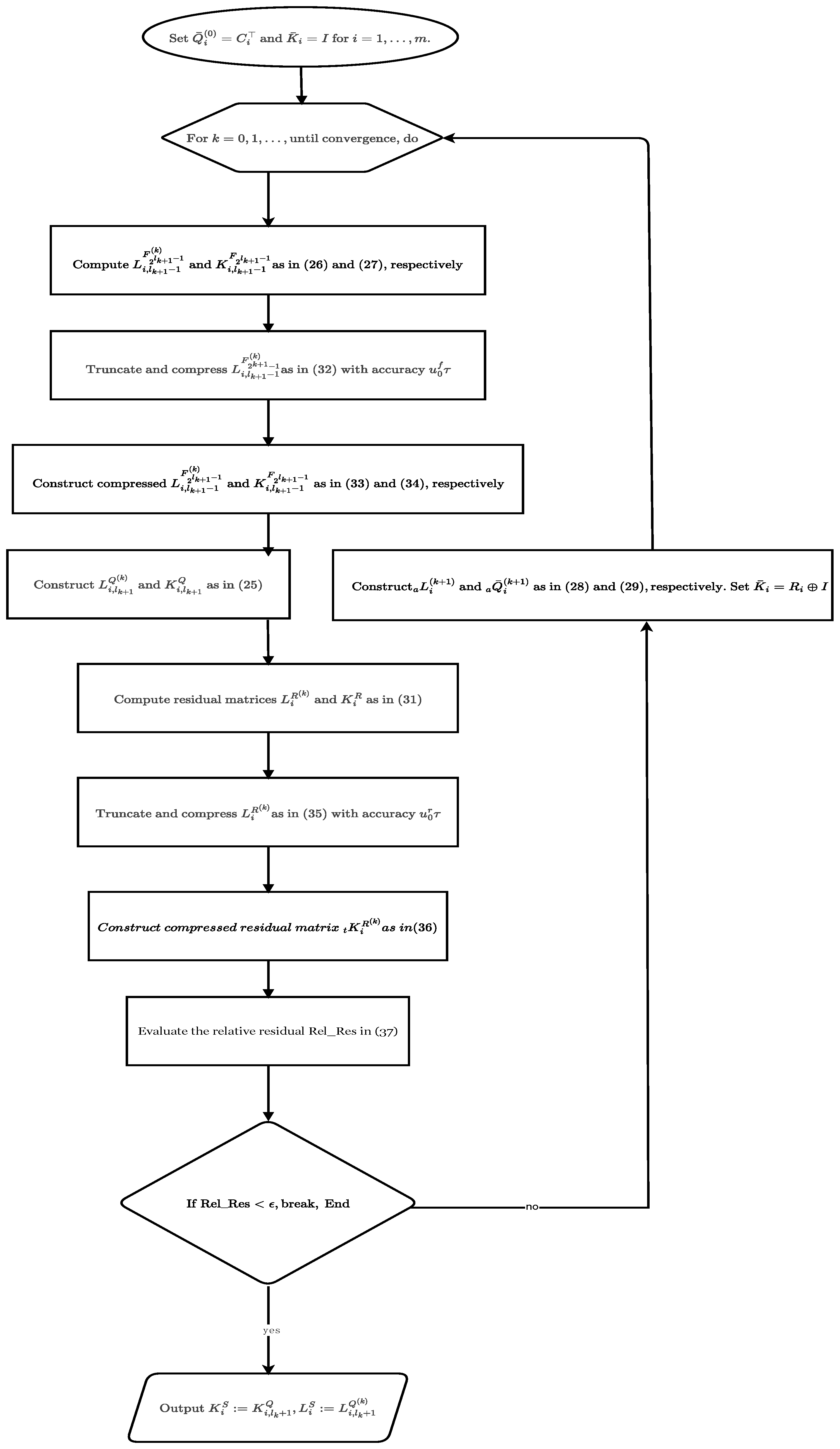
To further illustrate the convergence characteristics of the OSA used to solve each subproblem, we depict its convergence trajectories under various dimensions in Figure 2. In each subplot, the outer iterations 1 through 4 are represented by red, yellow, green, and orange, respectively. Within each color, a gradient from light to dark corresponds to increasing values drawn from the interval $(0,10)$. The concentric rings indicate logarithmic scales from ${10}^{-1}$ to ${10}^{-15}$. The convergence behavior of the OSA is marked by black circles, blue pentagrams, purple stars, and brown diamonds across the four outer iterations. From the number of concentric levels traversed by each marker, it is evident that the OSA achieves near-quadratic convergence across all subproblems. This reinforces the effectiveness of the proposed operator Newton framework in delivering rapid and robust convergence from inner iterations to the overall CDARE solution.

Example 2.

Consider a structural model of a vertically mounted stand, representative of machinery control systems. This model corresponds to a segment of a machine tool frame, where a series of guide rails is fixed along one surface to facilitate the motion of a tool slide during operation [28,31]. The geometry has been modeled and meshed using ANSYS, and the spatial discretization employs linear Lagrange elements within the finite element framework implemented in FEniCS.

The resulting system matrices are

$$\begin{array}{cc}{A}_1=r_{1}A\in {\mathbb{R}}^{16,626\times 16,626},& A_2=r_{2}A\in {\mathbb{R}}^{16,626\times 16,626},\\ B_1=B_2=B\in {\mathbb{R}}^{16,626\times 1}& R_1=R_2=1,\end{array}$$

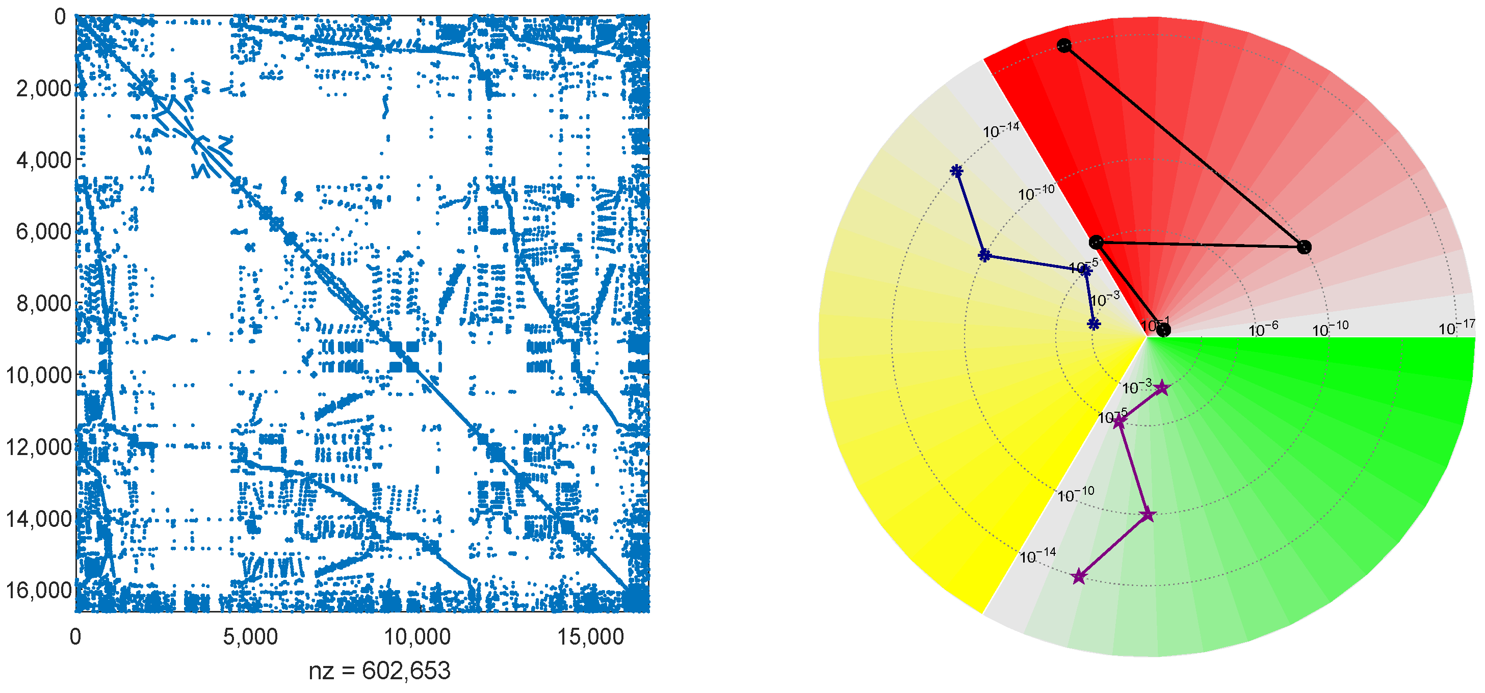
where random scalars $r_1,r_2\in (0,1)$ are used for certain parameterizations, and the vector B has 392 nonzero elements, with a maximum entry of at most $0.00251$. Due to the structural similarity between $A_1$ and $A_2$, only the sparsity pattern of $A_1$ is depicted on the left panel of Figure 3. Vectors $C_1$ and $C_2\in {\mathbb{R}}^{16,626}$ are mostly zero, with five nonzero entries located at rows (3341, 6743, 8932, 11,324, 16,563) for $C_1$ and (1046, 2436, 6467, 8423, 12,574) for $C_2$, respectively. Full matrix data are available from [27] and at the MOR Wiki repository (https://morwiki.mpi-magdeburg.mpg.de/morwiki/index.php/Vertical_Stand) (accessed on 30 July 2025). For this example, we set $m=2$ and define the mode transition probability matrix as $\Pi =\left(\begin{array}{cc}0.564& 0.436\\ 0.785& 0.215\end{array}\right)$.

We apply the ONM_lr algorithm to solve the resulting coupled CDARE. We omit the comparison with the standard Newton’s method incorporating the HODLR structure, as it is out of memory capacity during iterations at this problem dimension.

Table 4. CPU time and residual in Example 2.

N	It.	$\mathit{\delta }{\mathit{t}}_{\mathit{k}}$	${\mathit{t}}_{\mathit{k}}$	Rel_Res	NC
16,626	1	$0.036$	$0.036$	$1.74\times {10}^{-4}$	31
	2	$0.923$	$0.959$	$9.23\times {10}^{-9}$	68
	3	$1.731$	$2.691$	$2.58\times {10}^{-15}$	122

summarizes the numerical results of ONM_lr. The residuals decrease to $O\left({10}^{-15}\right)$ after only three outer iterations. The columns $t_k$ and $\delta t_k$ report the cumulative and per-iteration CPU time, respectively. The NC column shows that the column dimension of $L_{i,l_{k+1}}^{Q^{\left(k\right)}}$ increases by more than twice in the first iteration but grows more slowly in subsequent iterations. The Rel_Res column confirms that ONM_lr retains a quadratic convergence.

To further investigate the convergence of the OSA for the subproblems, we present their convergence histories in the right panel of Figure 3. The red, yellow, and green colors correspond to the first, second, and third subproblem solving, respectively, with increasing intensities representing values in $(0,10)$. Concentric circles indicate residual magnitudes from ${10}^{-1}$ to ${10}^{-18}$. The convergence trajectories are plotted using black circles, blue pentagrams, and purple stars. The number of magnitude levels traversed by these markers provides clear evidence of nearly quadratic convergence for the OSA. This validates the robustness and efficiency of the ONM_lr algorithm in conjunction with the OSA strategy.

Example 3.

Consider a semi-discretized heat transfer model arising from the optimal cooling of steel profiles in automated control systems, as studied in [27]. The dimension of the resulting dynamical system depends on the level of refinement applied to the computational mesh. Spatial discretization is performed using linear Lagrange elements via the ALBERTA-1.2 finite element toolbox [30].

We slightly modify the model matrices as follows:

$$\begin{array}{cc}{A}_1=r_1{\overline{A}}_1\in {\mathbb{R}}^{N\times N},& A_2=r_2{\overline{A}}_2\in {\mathbb{R}}^{N\times N},\\ B_1=B_2\in {\mathbb{R}}^{N\times 7},& C_1=C_2\in {\mathbb{R}}^{7\times N},\end{array}$$

where $\overline{A}=A/\parallel A\parallel$ and $\parallel A\parallel$ is estimated by ‘normest’ in Matlab. We take $r_1=0.98$ and $r_2=0.92$ for $N=20,209$ and $r_1=0.87$ and $r_2=0.97$ for $N=79,841$. $R_1=R_2=I_7$. In this experiment, we take $C_1=r_{3}C$ and $C_2=r_{4}C$ with $r_3$ and $r_4$ being random numbers in (0,1). Matrices $\overline{A}\in {\mathrm{R}}^{N\times N}$, $B\in {\mathrm{R}}^{N\times 1}$, and $C\in {\mathrm{R}}^{1\times N}$ can be found at [27], or the MOR Wiki repository (https://morwiki.mpi-magdeburg.mpg.de/morwiki/index.php/Steel_Profile) (accessed on 30 July 2025). The probability matrix is defined as $\Pi =\left(\begin{array}{cc}0.713& 0.287\\ 0.584& 0.416\end{array}\right)$.

To assess the performance of the proposed ONM_lr algorithm, we solve Equation (1) for two system sizes: $N=20,209$ and $N=79,841$. Again, we omit the comparison with the standard Newton’s method incorporating the HODLR structure, as it is out of memory capacity during iterations at this problem dimension. The numerical results of ONM_lr are reported in

Table 5. CPU time and residual in Example 3.

N	It.	$\mathit{\delta }{\mathit{t}}_{\mathit{k}}$	${\mathit{t}}_{\mathit{k}}$	Rel_Res	NC
20,209	1	$0.258$	$0.258$	$5.65\times {10}^{-4}$	48
	2	$2.843$	$3.101$	$1.53\times {10}^{-9}$	88
	3	$7.472$	$10.574$	$1.69\times {10}^{-15}$	103
79,841	1	$0.458$	$0.458$	$8.72\times {10}^{-4}$	48
	2	$5.098$	$5.556$	$2.34\times {10}^{-8}$	88
	3	$13.912$	$19.468$	$4.25\times {10}^{-15}$	101

. In both cases, ONM_lr attains a residual norm on the order of ${10}^{-15}$ within just three outer iterations. The cumulative CPU times are approximately 10.5 s and 19.5 s. The It. column records the number of outer iterations, while the NC column reflects the maximum number of columns in $L_{i,l_{k+1}}^{Q^{\left(k\right)}}$ at each step. The modest growth in NC, remaining below two times across iterations, highlights the efficiency of the truncation–compression (TC) strategy employed within both the outer ONM_lr iterations and the inner OSA iterations. Furthermore, the Rel_Res column confirms the quadratic convergence of ONM_lr.

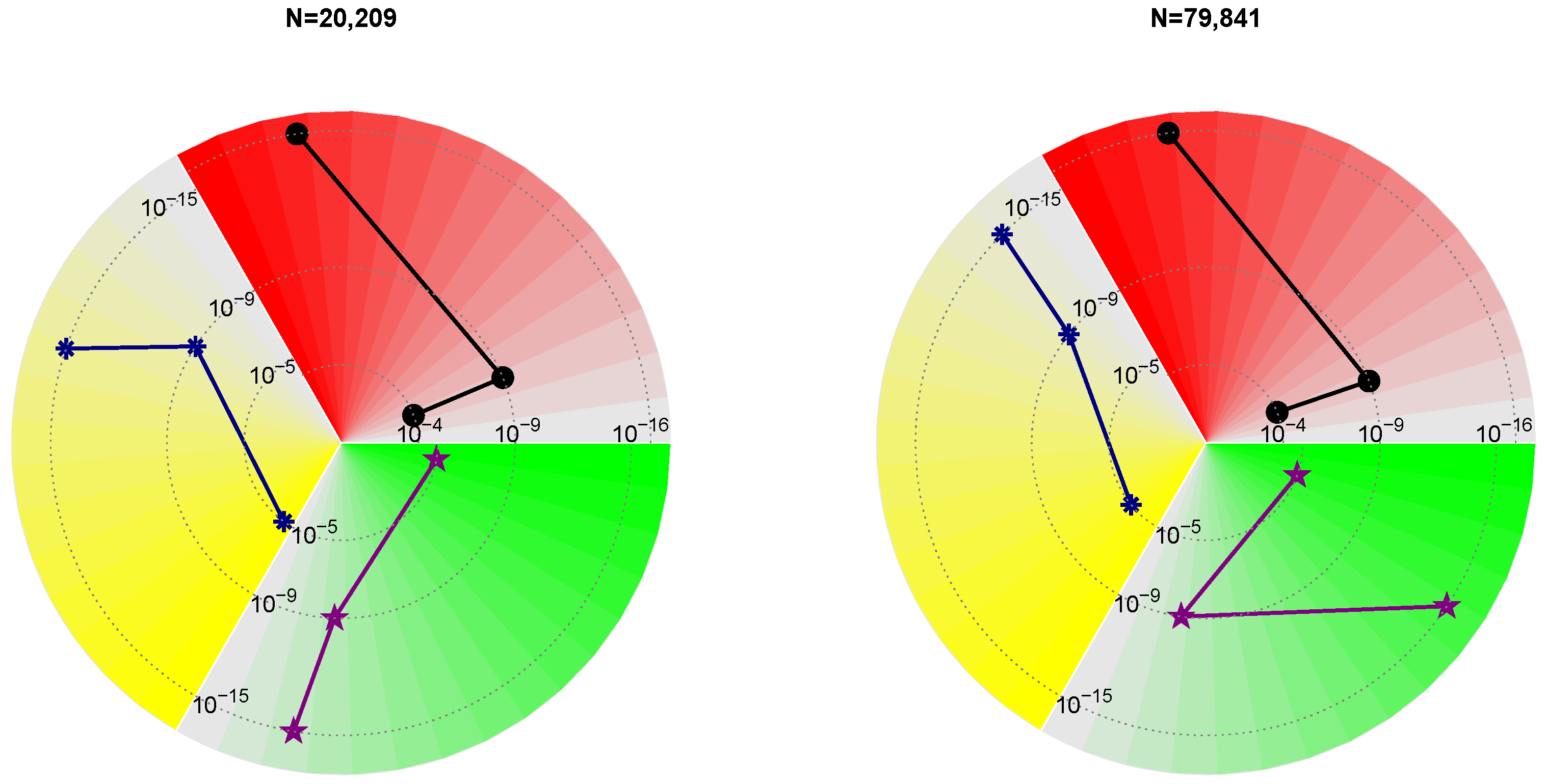
To further visualize the convergence characteristics of the subproblem solvers, we depict the residual histories for both problem sizes in the right panel of Figure 4. Each subplot uses red, yellow, and green markers to represent the first through third subproblem solving. Within each color, darker shades correspond to higher iteration indices. Concentric rings denote residual levels ranging from ${10}^{-1}$ to ${10}^{-16}$. The convergence paths of the operator Smith iteration are illustrated using black circles, blue pentagrams, and purple stars. The number of magnitude rings traversed by these markers clearly indicates that each subproblem is solved with nearly quadratic convergence. This further confirms the rapid and robust performance of the ONM_lr algorithm when combined with the OSA subproblem strategy.

6. Conclusions

We have developed an operator Newton method for computing the solutions to a class of coupled discrete-time algebraic Riccati equations (CDARE) arising from jump systems. The proposed framework leverages an inner operator Smith algorithm to solve subproblems, and under appropriate assumptions, guarantees locally quadratic convergence in both the inner and outer iterations. To efficiently address large-scale systems in engineering applications, we further present a low-rank variant, ONM_lr, which incorporates truncation and compression strategies to control memory and computational costs. Compared to the standard Newton’s method incorporating the HODLR structure [21,22] and the recently developed inverse-free fixed-point iterations [12,13], which require invertible constant matrices and therefore fail to accommodate low-rank structures in large-scale scenarios, the proposed ONM_lr algorithm demonstrates its effectiveness in handling large-scale problems through numerical experiments. However, when CDARE approaches the critical case, the presented ONM method tends to exhibit near-linear convergence, leading to a significant increase in computational time for large-scale problems. Overcoming this limitation is an important direction for further research and is currently under investigation. Another future research avenue may be to extend the ONM method to coupled continuous-time Riccati equations and other types of equations arising in large-scale stochastic jump systems.

References

1. Abou-Kandil, H.; Freiling, G.; Jank, G. On the solution of discretetime markovian jump linear quadratic control problems. Automatica 1995, 31, 765–768. [Google Scholar] [CrossRef]
2. Liu, Y.; Wang, Z.; Lin, X. Non-zero sum Nash game for discrete-time infinite Markov jump stochastic systems with applications. Axioms 2023, 12, 882. [Google Scholar] [CrossRef]
3. Do Costa, O.L.V.; Marques, R.P.; Fragoso, M.D. Discrete-Time Markov Jump Linear Systems; Springer: London, UK, 2005. [Google Scholar]
4. Zhou, B.; Duan, G.-R.; Li, Z.-Y. Gradient based iterative algorithm for solving coupled matrix equations. Syst. Control. Lett. 2009, 58, 327–333. [Google Scholar] [CrossRef]
5. Wang, Q.; Lam, J.; Wei, Y.; Chen, T. Iterative solutions of coupled discrete Markovian jump Lyapunov equations. Comput. Math. Appl. 2008, 55, 843–850. [Google Scholar] [CrossRef]
6. Wu, A.-G.; Duan, G.-R. New iterative algorithms for solving coupled Markovian jump Lyapunov equations. IEEE Trans. Autom. Control 2015, 60, 289–294. [Google Scholar]
7. Dragan, V.; Morozan, T.; Stoica, A.M. Robust Control of Discrete-time Linear Stochastic Systems; Springer: Berlin/Heidelberg, Germany, 2010. [Google Scholar]
8. Ivanov, I.G. Accelerated LMI solvers for the maximal solution to a set of discrete-time algebraic Riccati equations. Appl. Math. E-Notes 2012, 12, 228–238. [Google Scholar]
9. Ivanov, I.G. A method to solve the discrete-time coupled algebraic riccati equations. Appl. Math. Comput. 2008, 206, 34–41. [Google Scholar] [CrossRef]
10. Haghani, F.K.; Soleymani, F. An improved Schulz-type iterative method for matrix inversion with application. Trans. Inst. Meas. Control 2014, 36, 983–991. [Google Scholar] [CrossRef]
11. Dai, H.; Bai, Z.Z. On eigenvalue bounds and iteration methods for discrete algebraic riccati equations. J. Comput. Math. 2011, 29, 341–366. [Google Scholar] [CrossRef]
12. Jiang, K.-W.; Li, Z.; Zhang, Y. An inversion-free iterative algorithm with a scalar tuning parameter for coupled Riccati matrix equations arising in LQ optimal control of Markov jump systems. IEEE Trans. Autom. Control 2024, 70, 1913–1920. [Google Scholar] [CrossRef]
13. Li, Z.; Zhang, Y.; Wu, A.-G. An inversion-free iterative algorithm for riccati matrix equations in discrete-time markov jump systems. IEEE Trans. Autom. Control 2022, 67, 4754–4761. [Google Scholar] [CrossRef]
14. Feng, T.-T.; Chu, E.K.W. Newton’s method for coupled continuous-time algebraic Riccati equations. J. Appl. Math. Comput. 2024, 70, 1023–1042. [Google Scholar] [CrossRef]
15. Salama, A.; Gourishankar, V. A computational algorithm for solving a system of coupled algebraic matrix riccati equations. IEEE Trans. Comput. 1974, C-23, 100–102. [Google Scholar] [CrossRef]
16. Margenov, S.D.; Vulkov, L.G.; Wasniewski, J. (Eds.) Numerical Analysis and Its Applications. In Proceedings of the 4th International Conference (NAA 2008), Lozenetz, Bulgaria, 16–20 June 2008; Revised Selected Papers; Springer: Berlin/Heidelberg, Germany, 2009; Volume 5434. [Google Scholar]
17. Wang, L.; Zhu, Y.-L. A new inversion-free iterative algorithm for the discrete algebraic Riccati equation. IMA J. Math. Control Inf. 2024, 41, 149–164. [Google Scholar] [CrossRef]
18. Jerbi, H.; Alshammari, O.; Aoun, S.B.; Kchaou, M.; Simos, T.E.; Mourtas, S.D.; Katsikis, V.N. Hermitian solutions of the quaternion algebraic Riccati equations through zeroing neural networks with application to quadrotor control. Mathematics 2024, 12, 15. [Google Scholar] [CrossRef]
19. Escorcia, J.M.; Suazo, E. On blow-up and explicit soliton solutions for coupled variable coefficient nonlinear schrödinger equations. Mathematics 2024, 12, 2694. [Google Scholar] [CrossRef]
20. Yu, B.; Dong, N.; Hu, B.-Q. Operator Smith algorithm for coupled Stein equations from jump control systems. Axioms 2024, 13, 249. [Google Scholar] [CrossRef]
21. Massei, S.; Palitta, D.; Robol, L. Solving rank structured Sylvester and Lyapunov equations. SIAM J. Matrix Anal. Appl. 2018, 39, 1564–1590. [Google Scholar] [CrossRef]
22. Massei, S.; Robol, L.; Kressner, D. hm-toolbox: Matlab software for HODLR and HSS matrices. SIAM J. Sci. Comput. 2020, 42, C43–C68. [Google Scholar] [CrossRef]
23. Higham, N.J. Accuracy and Stability of Numerical Algorithms, 2nd ed.; SIAM: Philadephia, PA, USA, 2002. [Google Scholar]
24. Yu, B.; Dong, N.; Tang, Q. Factorized squared Smith method for large-scale Stein equations with high-rank terms. Automatica 2023, 154, 111057. [Google Scholar] [CrossRef]
25. Yu, B.; Fan, H.-Y.; Chu, E.K.-W. Large-scale algebraic Riccati equations with high-rank constant terms. J. Comput. Appl. Math. 2019, 361, 130–143. [Google Scholar] [CrossRef]
26. Higham, N.J. Functions of Matrices: Theory and Computation; SIAM: Philadelphia, PA, USA, 2008. [Google Scholar]
27. Korvink, G.; Rudnyi, B. Oberwolfach Benchmark Collection. In Dimension Reduction of Large-Scale Systems; Benner, P., Sorensen, D.C., Mehrmann, V., Eds.; Lecture Notes in Computational Science and Engineering; Springer: Berlin/Heidelberg, Germany, 2005; p. 45. [Google Scholar]
28. Lang, N. Numerical Methods for Large-Scale Linear Time-Varying Control Systems and related Differential Matrix Equations; Logos-Verlag: Berlin, Germany, 2018. [Google Scholar]
29. Ober, R.J. Asymptotically Stable All-Pass Transfer Functions: Canonical Form, Parametrization and Realization. IFAC Proc. Vol. 1987, 20, 181–185. [Google Scholar] [CrossRef]
30. Schmidt, A.; Siebert, K. Design of Adaptive Finite Element Software—The Finite Element Toolbox ALBERTA; Lecture Notes in Computational Science and Engineering; Springer: Berlin/Heidelberg, Germany, 2005; Volume 42. [Google Scholar]
31. Chahlaoui, Y.; Van Dooren, P. Benchmark examples for model reduction of linear time-invariant dynamical systems, dimension reduction of large-scale systems. In Dimension Reduction of Large-Scale Systems; Springer: Berlin/Heidelberg, Germany, 2005; Volume 45, pp. 379–392. [Google Scholar]
Figure 1. Flowchart of the low-rank structured ONM equipped with truncation and compression.
Axioms 14 00601 g001
Figure 2. Residual history of operator Smith iteration in solving each subproblem of Example 1.
Axioms 14 00601 g002
Figure 3. The discretized matrix A and residual history of OSI in solving each subproblem of Example 2.
Axioms 14 00601 g003
Figure 4. Residual history of OSA in each subproblem of Example 3.
Axioms 14 00601 g004