Article

Improved Bounds for Integral Jensen’s Inequality Through Fifth-Order Differentiable Convex Functions and Applications

1
Centre for Advanced Studies in Pure and Applied Mathematics, Bahauddin Zakariya University, Multan 60800, Pakistan
2
Department of Mathematics, Faculty of Science, Taif University, Taif 21944, Saudi Arabia
*
Author to whom correspondence should be addressed.
These authors contributed equally to this work.
Axioms 2025, 14(8), 602; https://doi.org/10.3390/axioms14080602 (registering DOI)
Submission received: 17 June 2025 / Revised: 24 July 2025 / Accepted: 29 July 2025 / Published: 2 August 2025
(This article belongs to the Special Issue Theory and Application of Integral Inequalities, 2nd Edition)

Abstract

The main objective of this research is to obtain interesting estimates for Jensen’s gap in the integral sense, along with their applications. The convexity of a fifth-order absolute function is used to established proposed estimates of Jensen’s gap. We performed numerical computations to compare our estimates with previous findings. With the use of the primary findings, we are able to obtain improvements of the Hölder inequality and Hermite–Hadamard inequality. Furthermore, the primary results lead to some inequalities for power means and quasi-arithmetic means. We conclude by outlining the information theory applications of our primary inequalities.
MSC:
26A51; 26D15; 68P30

1. Introduction

The study of convex functions is a great way to experience the elegance and allure of sophisticated mathematics. Studying convex functions helps one to understand the efficiency and order that are inherent in mathematical structures, in addition to solving equations. A convex function [1] is defined as follows:
Definition 1.
A function K : [ a , b ] R is said to be a convex, if the relation
K h z 1 + ( 1 h ) z 2 h K ( z 1 ) + ( 1 h ) K ( z 2 ) ,
holds, for all z 1 , z 2 [ a , b ] and h [ 0 , 1 ] . K is said to be concave over [ τ 1 , τ 2 ] if the aforementioned inequality is true in the reverse sense.
Convex functions have several generalizations. Some recent generalizations include pseudo-convex functions [2], invex functions [3], quasi-convex functions [4], preinvex functions [5], and E-convex functions [6]. It is notable that convexity yields a number of creative ideas on mathematical inequalities and their applications. In the literature on inequalities, Jensen’s inequality extends the notion of convexity to expectations and weighted averages. Jensen’s inequality is one of the most famous and widely used inequalities in the field of mathematical inequalities. Jensen’s inequality [1] in the discrete form is stated as follows:
Theorem 1.
Let I R and K be a convex function on I . If z l I and h l > 0 for l = 1 , 2 , , n with H = l = 1 n h l , then
K 1 H l = 1 n h l z l 1 H l = 1 n h l K ( z l ) .
If the function K is concave on I , then Inequality (2) will hold in the reverse direction.
Jensen’s inequality [7] in continuous form can be described as follows:
Theorem 2.
Assume that ϕ , φ : [ a , b ] R are any integrable functions with φ ( z ) 0 and ϕ ( z ) I for all z [ τ 1 , τ 2 ] , Also, suppose that φ ¯ = τ 1 τ 2 φ ( z ) d z > 0 . If K ( ϕ ( z ) ) is an integrable function, then
K 1 φ ¯ τ 1 τ 2 φ ( z ) ϕ ( z ) d z 1 φ ¯ τ 1 τ 2 φ ( z ) K ( ϕ ( z ) ) d z ,
for each convex function K : I R . If K is concave, then (2) reverses.
Jensen’s inequality is crucial because it may be used to derive other classical inequalities, such as the Hölder’s, arithmetic–geometric, Minkowski’s, Young’s, and the Hermite–Hadamard inequalities. The Hermite–Hadamard inequality can be considered as an improvement of the concept of convexity and it is defined as follows:
Definition 2.
Let K : I = [ a , b ] R R be an integrable convex function. Then,
K a + b 2 1 b a a b K ( z ) d z K ( a ) + K ( b ) 2 .
Both inequalities hold in the reverse direction if K is concave.
Hölder’s inequality is a fundamental inequality in mathematics used to bound the integral or sum of a product of functions.
Definition 3.
Let p > 1 and 1 p + 1 q = 1 . If K and g are real functions defined on [ a , b ] and if K p and g q are integrable functions on [ a , b ] , then
a b K ( z ) g ( z ) d z a b K ( z ) p d z 1 p a b g ( z ) q d z 1 q ,
with equality holding if and only if A K ( z ) p = B g ( z ) q almost everywhere, where A and B are constants.
In addition, Talylor’s theorem with the integral remainder form has always been helpful in deriving the new bounds of Jensen’s inequality, which is stated as follows:
Theorem 3.
Let K be a function with ( n + 1 ) continuous derivatives on the interval between a and x . Then,
K ( z ) = K ( a ) + ( z a ) K ( a ) + ( z a ) 2 2 ! K ( a ) + + ( z a ) n n ! K ( n ) ( a ) + R n ( z ) ,
where the remainder term R n ( z ) is given by the integral form
R n ( z ) = 1 n ! a z K ( n + 1 ) ( t ) ( z t ) n d t .
Setting n = 4 , the Equation (6) becomes
K ( z ) = K ( a ) + ( z a ) K ( a ) + ( z a ) 2 2 ! K ( a ) + ( z a ) 3 3 ! K ( a ) + ( z a ) 4 4 ! K ( 4 ) ( a ) + 1 24 a z K ( 5 ) ( t ) ( z t ) 5 d t .
Also, Jensen’s inequality has been used to address several problems in different fields of science and technology, e.g., engineering [8], information science [9], mathematical statistics [10], and financial economics [11]. Regarding its generalizations, improvements, refinements, converses, etc., an extensive body of literature is available. Furthermore, Jensen’s inequality has also been demonstrated for several generalized classes of convex functions, including s-convex [12], coordinated convex [13], P-convex [14], h-convex [15], and six-convex functions [16]. Dragomir [17] discussed a refinement of the prominent Jensen inequality by taking the convex function over linear space. Khan et al. [7] obtained new estimates of Jensen’s gap by using the green function. Deng et al. [18] used some majorization results to provide refinements of the discrete Jensen inequality. Moreover, they also demonstrated the applicability of the improved Jensen inequality to information theory, power means, and quasi-arithmetic means. Using four-convexity, Ullah et al. [19] improved Jensen’s inequality in both continuous and discrete forms. Through the notion of majorization, Saeed et al. [20] refined the well-known integral Jensen’s inequality. These were used to refine the Hermite–Hadamard and Hölder inequalities. Zhu and Yang [21] examined the stability of discrete time delay systems in 2008 by applying Jensen’s inequality. Khan et al. [22] gave new estimates of Jensen difference by using the absolute convexity of the first differentiable function given as follows:
Theorem 4.
Consider a differentiable function K : [ c , d ] R such that f is a convex function and let w ( x ) , T ( x ) be two integrable functions defined on [ c , d ] such that T ( x ) [ c , d ] for all x [ c , d ] and c d w ( x ) d x = w ¯ 0 . Also, assume that T ¯ = 1 w ¯ c d w ( x ) ( T ( x ) ) d x [ c , d ] . Then,
K ( T ¯ ) 1 w ¯ c d w ( x ) K ( T ( x ) ) d x 1 2 w ¯ c d w ( x ) T ¯ T ( x ) K ( T ¯ ) + K ( T ( x ) ) d x .
Sohail et al. [23] presented new refinements of Jensen’s inequality using absolute convexity of thrice differentiable functions, supported by numerical comparisons and applications to classical inequalities, means, and divergences.
Theorem 5.
Assume that the function K : [ a . b ] R is thrice differentiable with K being a convex function and w ( x ) = [ c , d ] ( , ) , T : [ c , d ] [ a , b ] being any integrable function. Further presume that w ¯ = c d w ( x ) d x 0 and T ¯ = 1 w ¯ c d w ( x ) ( T ( x ) ) d x [ c , d ] . Then,
K ( T ¯ ) 1 w ¯ c d w ( x ) K ( T ( x ) ) d x 1 12 w ¯ c d w ( x ) T ¯ T ( x ) 3 3 K ( 3 ) ( T ¯ ) + K ( 3 ) ( T ( x ) ) 2 d x + 1 2 K ( 2 ) ( T ¯ ) w ¯ c d w ( x ) T ¯ T ( x ) 2 d x .
The primary goal of this study is to provide new Jensen gap estimations, present applications of these estimates in the theory of means and information theory, and to refine classical inequalities. For this purpose, we use a function whose absolute fifth-order derivative is convex. In many classical settings, second- or fourth-order bounds suffice; however, in the application domains, fifth-order derivative-based bounds offer substantial advantages. These bounds become particularly valuable in systems or models exhibiting strong nonlinear behavior, non-Gaussianity, or where tight bounds are essential (e.g., high-precision numerical methods).
The layout of this paper is as follows: the main findings are presented in Section 2. The importance of these findings is covered in Section 3, with particular attention paid to the bounds that are determined with the conditions on the function. Applications of the main findings to the Hölder and Hermite–Hadamard inequalities are presented in Section 4, such as graphical result verification, whereas Section 5 includes mean theory applications. We examine information theory applications in Section 6.

2. Main Results

Let us start this section by obtaining the following theorem that provides enhancement of Jensen’s inequality.
Theorem 6.
Suppose that the function K : [ a , b ] R is fifth differentiable, with K ( 5 ) being a convex function and w : [ c , d ] ( , ) , χ : [ c , d ] [ a , b ] being any integrable function. Further, assume that w ¯ = c d w ( x ) d x 0 and χ ¯ = 1 w ¯ c d w ( x ) χ ( x ) d x [ a , b ] . Then,
K ( χ ¯ ) 1 w ¯ c d w ( x ) K ( χ ( x ) ) d x 1 24 w ¯ c d w ( x ) χ ¯ χ ( x ) 5 5 K ( 5 ) ( χ ¯ ) + K ( 5 ) ( χ ( x ) ) 30 d x + K ( 4 ) ( χ ¯ ) 24 w ¯ c d w ( x ) χ ¯ χ ( x ) 4 d x + 1 6 K ( χ ¯ ) w ¯ c d w ( x ) χ ¯ χ ( x ) 3 d x + 1 2 K ( χ ¯ ) w ¯ c d w ( x ) χ ¯ χ ( x ) 2 d x .
Proof. 
Without loss of generality, assume that χ ¯ χ ( x ) . Using the integral form of Taylor’s expansion (7) in 1 w ¯ c d w ( x ) K ( χ ( x ) ) d x , we get
1 w ¯ c d w ( x ) K ( χ ( x ) ) d x = K ( χ ¯ ) + K ( χ ¯ ) w ¯ c d w ( x ) χ ( x ) χ ¯ d x + 1 2 w ¯ K ( χ ¯ ) c d w ( x ) χ ( x ) χ ¯ 2 d x + 1 6 w ¯ K ( χ ¯ ) c d w ( x ) χ ( x ) χ ¯ 3 d x + 1 24 w ¯ K 4 ( χ ¯ ) c d w ( x ) χ ( x ) χ ¯ 4 d x + 1 24 w ¯ c d w ( x ) χ ¯ χ ( x ) χ ( x ) a 4 K ( 5 ) ( a ) d a d x .
Now, by using the change in the variable a = t χ ¯ + ( 1 t ) χ ( x ) for t [ 0 , 1 ] , we obtain
1 w ¯ c d w ( x ) K ( χ ( x ) ) d x = K ( χ ¯ ) + K ( χ ¯ ) w ¯ c d w ( x ) χ ( x ) χ ¯ d x
+ 1 2 w ¯ K ( χ ¯ ) c d w ( x ) χ ( x ) χ ¯ 2 d x + 1 6 w ¯ K ( χ ¯ ) c d w ( x ) χ ( x ) χ ¯ 3 d x + 1 24 w ¯ K ( 4 ) ( χ ¯ ) c d w ( x ) χ ( x ) χ ¯ 4 d x 1 24 w ¯ c d w ( x ) χ ¯ χ ( x ) 5 0 1 t 4 K ( 5 ) ( t χ ¯ + ( 1 t ) χ ( x ) ) d t d a .
This implies that
K ( χ ¯ ) 1 w ¯ c d w ( x ) K ( χ ( x ) ) d x = 1 24 w ¯ c d w ( x ) χ ¯ χ ( x ) 5 0 1 t 4 K ( 5 ) ( t χ ¯ + ( 1 t ) χ ( x ) ) d t d x K K ( 4 ) ( χ ¯ ) 24 w ¯ c d w ( x ) χ ¯ χ ( x ) 4 d x + K ( χ ¯ ) 6 w ¯ c d w ( x ) χ ¯ χ ( x ) 3 d x K ( χ ¯ ) 2 w ¯ c d w ( x ) χ ¯ χ ( x ) 2 d x .
Taking the absolute value of the identity (9), and subsequently using triangular inequality, we get
K ( χ ¯ ) 1 w ¯ c d w ( x ) K ( χ ( x ) ) d x 1 24 c d w ( x ) χ ¯ χ ( x ) 5 w ¯ 0 1 t 4 K ( 5 ) ( t χ ¯ + ( 1 t ) χ ( x ) ) d t d x + K K ( 4 ) ( χ ¯ ) 24 c d w ( x ) χ ¯ χ ( x ) 4 w ¯ d x + 1 6 K ( χ ¯ ) c d w ( x ) χ ¯ χ ( x ) 3 w ¯ d x + 1 2 K ( χ ¯ ) c d w ( x ) χ ¯ χ ( x ) 2 w ¯ d x .
Taking into consideration that K ( 5 ) is convex, applying the convexity of K ( 5 ) in (10), we get
K ( χ ¯ ) 1 w ¯ c d w ( x ) K ( χ ( x ) ) d x 1 24 c d w ( x ) χ ¯ χ ( x ) 5 w ¯ 0 1 t 4 . t K ( 5 ) ( χ ¯ ) + t 4 . ( 1 t ) K ( 5 ) ( χ ( x ) ) d t d x + K K ( 4 ) ( χ ¯ ) 24 c d w ( x ) χ ¯ χ ( x ) 4 w ¯ d x + 1 6 K ( χ ¯ ) c d w ( x ) χ ¯ χ ( x ) 3 w ¯ d x + 1 2 K ( χ ¯ ) c d w ( x ) χ ¯ χ ( x ) 2 w ¯ d x = 1 24 c d w ( x ) χ ¯ χ ( x ) 5 w ¯ K ( 5 ) ( χ ¯ ) 0 1 t 5 d t + K ( 5 ) ( χ ( x ) ) 0 1 ( t 4 t 5 ) d t d x + K ( 4 ) ( χ ¯ ) 24 c d w ( x ) χ ¯ χ ( x ) 4 w ¯ d x + 1 6 K ( χ ¯ ) c d w ( x ) χ ¯ χ ( x ) 3 w ¯ d x
+ 1 2 K ( χ ¯ ) c d w ( x ) χ ¯ χ ( x ) 2 w ¯ d x = 1 24 w ¯ c d w ( x ) χ ¯ χ ( x ) 5 1 6 K ( 5 ) ( χ ¯ ) + 1 30 K ( 5 ) ( χ ( x ) ) d x + K ( 4 ) ( χ ¯ ) 24 w ¯ c d w ( x ) χ ¯ χ ( x ) 4 d x + 1 6 K ( χ ¯ ) w ¯ c d w ( x ) χ ¯ χ ( x ) 3 d x + 1 2 K ( χ ¯ ) w ¯ c d w ( x ) χ ¯ χ ( x ) 2 d x .
Upon simplifying (11), we get (8). □
Remark 1.
A function with a convex fifth derivative does not necessarily imply that the original function is convex. While it is true that a convex function has a second derivative that is non-negative, and a function with a convex second derivative is convex, convexity alone does not guarantee any specific behavior for higher-order derivatives, especially beyond the second derivative.
The convexity or concavity of K ( 5 ) ( x ) is not guaranteed for all convex functions but may arise under certain conditions such as additional regularity conditions, e.g., f C 6 or if f 5 is monotonic and preserves the sign on the domain and f 5 x is non-negative. For specific function classes (e.g., exponentials, power functions, polynomials), the convexity of f 5 x can be explicitly determined by direct computation e.g., for f x = e a x , f 5 x is convex if a > 0 .
The following theorem uses concave functions to further improve the Jensen inequality.
Theorem 7.
Let K : [ a , b ] R be any function such that K ( 5 ) exists. Additionally, suppose that w : [ c , d ] ( , ) and χ : [ c , d ] [ a , b ] are integrable functions with w ¯ = c d w ( x ) d x 0 and χ ¯ = 1 w ¯ c d w ( x ) χ ( x ) d x [ a , b ] . If K ( 5 ) is a concave function, then
K ( χ ¯ ) 1 w ¯ c d w ( x ) K ( χ ( x ) ) d x 1 120 c d w ( x ) χ ¯ χ ( x ) 5 w ¯ K ( 5 ) 5 χ ¯ + χ ( x ) 6 d x + K ( 4 ) ( χ ¯ ) 24 c d w ( x ) χ ¯ χ ( x ) 4 w ¯ d x + 1 6 K ( χ ¯ ) c d w ( x ) χ ¯ χ ( x ) 3 w ¯ d x + 1 2 K ( χ ¯ ) c d w ( x ) χ ¯ χ ( x ) 2 w ¯ d x .
Proof. 
From (10), we infer
K ( χ ¯ ) 1 w ¯ c d w ( x ) K ( χ ( x ) ) 1 24 c d w ( x ) χ ¯ χ ( x ) 5 w ¯ 0 1 t 4 K ( 5 ) ( t χ ¯ + ( 1 t ) χ ( x ) ) d t d x 5 0 1 t 4 d t + K ( 4 ) ( χ ¯ ) 24 c d w ( x ) χ ¯ χ ( x ) 4 w ¯ d x + 1 6 K ( χ ¯ ) c d w ( x ) χ ¯ χ ( x ) 3 w ¯ d x + 1 2 K ( χ ¯ ) c d w ( x ) χ ¯ χ ( x ) 2 w ¯ d x .
Given that the function K ( 5 ) is concave on I, the integral Jensen inequality is applied on the right side of (13), and we get
K ( χ ¯ ) 1 w ¯ c d w ( x ) K ( χ ( x ) ) d x 1 120 c d w ( x ) χ ¯ χ ( x ) 5 w ¯ K ( 5 ) 0 1 t 4 ( t χ ¯ + ( 1 t ) χ ( x ) ) d t 0 1 t 4 d t d x + K ( 4 ) ( χ ¯ ) 24 c d w ( x ) χ ¯ χ ( x ) 4 w ¯ d x + 1 6 K ( χ ¯ ) c d w ( x ) χ ¯ χ ( x ) 3 w ¯ d x + 1 2 K ( χ ¯ ) c d w ( x ) χ ¯ χ ( x ) 2 w ¯ d x .
Finally, calculating the integral in (14), we get (12). □

3. Importance of Main Results

This section examines the impact of observed improvements in the bounds obtained from Theorem 6 and 7 in relation to earlier research findings.

3.1. Functions Fit the Criteria

In the literature, we may find functions for which the first- to fourth-order derivatives in terms of absolute values are not convex. Below is an illustration of one of these functions. Let us consider
K ( x ) = x 6 x 5 , x [ 1 , 1 ] .
Now, we can find the absolute value of the function of first- to fourth-order derivatives.
K ( x ) = 6 x 5 5 x 4 , x [ 1 , 1 ] .
K ( x ) = 30 x 4 20 x 3 , x [ 1 , 1 ] .
K ( x ) = 120 x 3 60 x 2 , x [ 1 , 1 ] .
K ( 4 ) ( x ) = 360 x 2 120 x , x [ 1 , 1 ] .
These functions are not convex, whereas the absolute value function of the fifth-order derivative is convex.
K ( 5 ) ( x ) = 720 x 120 , x [ 1 , 1 ] .
Figure 1 provides an illustration of this, demonstrating that the fifth-order absolute function is convex, but the first- to fourth-order absolute functions are not. This demonstrates the special contribution that our article makes.

3.2. Numerical Estimates for the Jensen Difference

In this part, we perform numerical experiments to show the importance of our main results over other results in the literature. In the first example, a parameter has given different values to check the bounds and are compared in Table 1 and Table 2.
Example 1.
Let K ( x ) = exp ( a x ) , x [ 0 , 1 ] where a > 0 . Therefore, using the inequality (8) for w ( x ) = 1 and χ ( x ) = x , where x [ 0 , 1 ]
With the previously described data and the specific function in Inequality (8) obtained by Khan et al. [22], we arrive at
As shown, Jensen’s difference estimates provided in this study are better than the estimates achieved from [22].
Example 2.
Let K ( x ) = ln ( 1 + x ) for x [ 0 , 1 ] . Then K ( 5 ) ( x ) = 24 ( 1 + x ) 5 , which is a convex function on the given interval. By applying Inequality (8) with the choices w ( x ) = 1 and χ ( x ) = x , we obtain the estimate
0.019175 0.01965 .
Furthermore, since K ( 3 ) ( x ) = 24 ( 1 + x ) 5 is also a convex function on [ 0 , 1 ] , using Inequality (2.1) from article [23], we derive the estimate as
0.019175 0.02206 .
Additionally, as K ( x ) = 1 ( 1 + x ) is also a convex function, applying Inequality (2.24) from article [22], we obtain
0.019175 0.171712 .
The results in (15)–(17) clearly demonstrate that the estimates derived in the present paper provide significantly sharper bounds compared to those obtained using the previously established Inequality (17) shows that estimates provided in this paper provide much better results.

4. Applications to Hölder and Hermite–Hadamard Inequalities

Hölder’s inequality is a fundamental result in mathematical analysis with widespread applications in various fields. e.g., functional analysis, probability theory, optimization, and physics. It makes it easier to explore functions in various spaces. One can even use it to nail down key points in probability and statistics, tweak machine learning models, and tackle hands-on problems in physics and engineering. On the other hand, the Hermite–Hadamard inequality refines the concept of convexity. In this section, we present applications of our obtained bounds to Holder’s and Hermite–Hadamard inequalities for specific choices of the underlying functions.
Proposition 1.
Let γ and η be two positive functions such that η p , γ q and η γ are integrable. Also, assume that p , q > 1 with 1 p + 1 q = 1 . If p ( 1 , 5 ] [ 6 , ] , then
c d γ q d x 1 q c d η p d x 1 p c d η γ d x p ( p 1 ) ( p 2 ) ( p 3 ) ( p 4 ) 720 c d γ q c d η γ d x c d γ q d x η γ q p 5 5 c d η γ d x c d γ q d x p 5 + ( η γ q p ) p 5 d x + p ( p 1 ) ( p 2 ) ( p 3 ) 24 c d η γ d x c d γ q d x p 4 c d γ q c d η γ d x c d γ q d x η γ q p 4 d x + p ( p 1 ) ( p 2 ) 6 1 c d γ q d x c d η γ d x p 3 c d γ q c d η γ d x c d γ q d x η γ q p 3 d x + p ( p 1 ) 2 1 c d γ q d x c d η γ d x p 2 c d γ q c d η γ d x c d γ q d x η γ q p 2 d x 1 P c d γ q d x 1 q .
Proof. 
Take the function K ( x ) = x p , x > 0 , then by the successive differentiation of the given function, we get K ( x ) = p ( p 1 ) x p 2 and K ( 5 ) ( x ) = p ( p 1 ) ( p 2 ) ( p 3 ) ( p 4 ) ( p 5 ) ( p 6 ) x p 7 . Clearly, both K ( x ) and K ( 5 ) ( x ) are nonnegative on ( 0 , ) for p ( 1 , 5 ] [ 6 , ] , which substantiate the convexity of K ( x ) as well as convexity of K ( 5 ) ( x ) . Based on this, using (8) for K ( x ) = x p , w ( x ) = γ q , χ ( x ) = η γ q p and then assuming power 1 p , we get
c d γ q d x p 1 c d η p d x c d η γ d x p 1 p p ( p 1 ) ( p 2 ) ( p 3 ) ( p 4 ) 720 c d γ q c d η γ d x c d γ q d x η γ q p 5 5 c d η γ d x c d γ q d x p 5 + ( η γ q p ) p 5 d x + p ( p 1 ) ( p 2 ) ( p 3 ) 24 c d η γ d x c d γ q d x p 4 c d γ q c d η γ d x c d γ q d x η γ q p 4 d x + p ( p 1 ) ( p 2 ) 6 1 c d γ q d x c d η γ d x p 3 c d γ q c d η γ d x c d γ q d x η γ q p 3 d x + p ( p 1 ) 2 1 c d γ q d x c d η γ d x p 2 c d γ q c d η γ d x c d γ q d x η γ q p 2 d x 1 p c d γ q d x 1 q .
Since the inequality k 1 l k 2 l < ( k 1 k 2 ) l holds for l [ 0 , 1 ] and 0 k 1 k 2 , using this inequality for k 1 = c d γ q d x p 1 c d η p d x and k 2 = c d η γ d x p and l = 1 p , we get
c d γ q d x 1 q c d η p d x 1 p c d η γ d x c d γ q d x p 1 c d η p d x c d η γ d x p 1 p .
By comparing Inequalities (19) and (20), we arrive at Inequality (18). □
Proposition 2.
Let γ and η be two positive functions such that η p , η q and η γ are integrable functions and p ( 0 , 1 ) with q = p p 1 . If 1 p ( 1 , 5 ] [ 6 , ] , then
c d η γ d x c d η p d x 1 p c d γ q d x 1 q ( 1 p ) ( 1 p 1 ) ( 1 p 2 ) ( 1 p 3 ) ( 1 p 4 ) 720 c d γ q c d η p d x c d γ q d x η γ q p 5 5 c d η p d x c d γ q d x + ( η p γ q ) 1 p 5 d x + ( 1 p ) ( 1 p 1 ) ( 1 p 2 ) ( 1 p 3 ) 24 c d η p d x c d γ q d x 1 p 4 c d γ q c d η p d x c d γ q d x η p γ q 4 d x + ( 1 p ) ( 1 p 1 ) ( 1 p 2 ) 6 c d η p d x c d γ q d x 1 p 3 c d γ q c d η p d x c d γ q d x η p γ q 3 d x
+ ( 1 p ) ( 1 p 1 ) 2 c d η p d x c d γ q d x 1 p 2 c d γ q c d η p d x c d γ q d x η p γ q 2 d x .
Proof. 
Consider a function K ( x ) = x 1 p , where x > 0 . Then K ( x ) = 1 p ( 1 p 1 ) x 1 p 2 and K ( 5 ) ( x ) = 1 p ( 1 p 1 ) ( 1 p 2 ) ( 1 p 3 ) ( 1 p 4 ) ( 1 p 5 ) ( 1 p 6 ) x p 7 . It is evident that both K ( x ) and K ( 5 ) ( x ) are nonnegative on ( 0 , ) for 1 p ( 1 , 5 ] [ 6 , ] , supporting the convexity of K ( x ) and convexity of K ( 5 ) ( x ) . Therefore, we use (8) for K ( x ) = x 1 p , w ( x ) = γ q , χ ( x ) = η p γ q to obtain (21).
c d η γ d x c d γ q d x c d η p d x 1 p c d γ q d x 1 p ( 1 p ) ( 1 p 1 ) ( 1 p 2 ) ( 1 p 3 ) ( 1 p 4 ) 720 c d γ q d x c d γ q 1 c d γ q d x c d η p d x η γ q p 5 5 1 c d γ q d x c d η p d x + ( η p γ q ) 1 p 5 d x + ( 1 p ) ( 1 p 1 ) ( 1 p 2 ) ( 1 p 3 ) 24 c d γ q d x
1 c d γ q d x c d η p d x 1 p 4 c d γ q 1 c d γ q d x c d η p d x η p γ q 4 d x + ( 1 p ) ( 1 p 1 ) ( 1 p 2 ) 6 c d γ q d x 1 c d γ q d x c d η p d x 1 p 3 c d γ q 1 c d γ q d x c d η p d x η p γ q 3 d x + ( 1 p ) ( 1 p 1 ) 2 c d γ q d x 1 c d γ q d x c d η p d x 1 p 2 c d γ q 1 c d γ q d x c d η p d x η p γ q 2 d x .
Now, multiplying both sides of Inequality (22) by c d γ q d x , we get Inequality (21). □
Let us consider an example for the estimates obtained from Proposition 1.
Example 3.
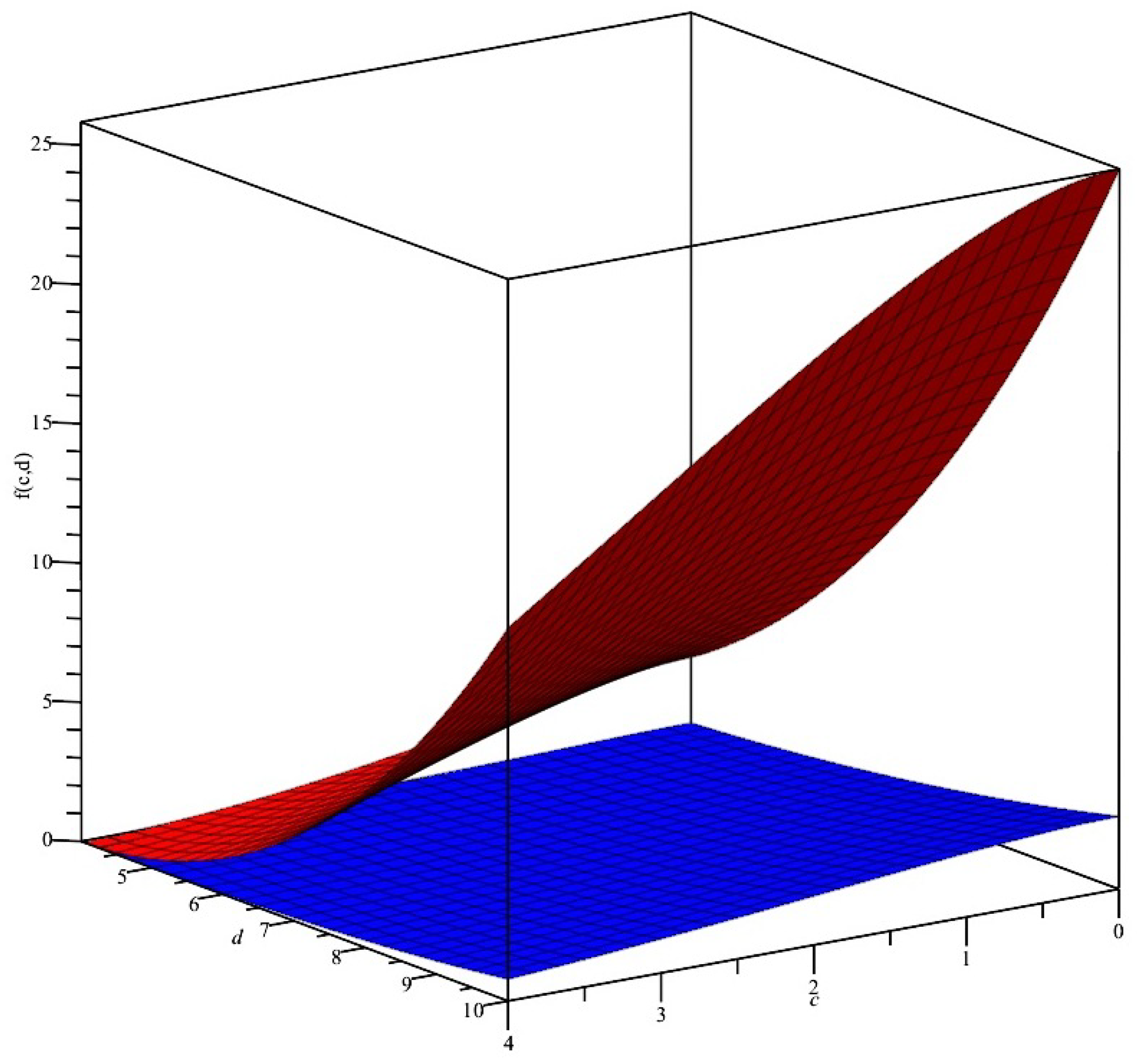
Take γ ( x ) = x 1 2 , η ( x ) = x , p = 2 , q = 2 , a = c [ 0 , 4 ] , b = d ( 4 , 10 ] such that d > c in (18). Using the above values for Inequality (18), we get
L . H . S = b 3 a 3 3 1 2 b 2 a 2 2 1 2 2 5 b 2.5 a 2.5
R . H . S = 8 25 b 2.5 a 2.5 2 b 2 a 2 + b 3 a 3 3 16 25 b 2.5 a 2.5 2 b 2 a 2 1 2 b 2 a 2 2 1 2 .
These estimates are visualized in Figure 2 below.
Proposition 3.
Let η , γ : [ β 1 , β 2 ] be any functions and p , q > 1 with 1 p + 1 q = 1 . Additionally, assume that γ q , η p , γ η and γ η q p are integrable over [ β 1 , β 2 ] . If p ( 5 , 6 ) , then
c d γ q d x 1 q c d η p d x 1 p c d η γ d x p ( p 1 ) ( p 2 ) ( p 3 ) ( p 4 ) 120 c d γ q c d η γ d x c d γ q d x η γ q p 5 5 6 c d η γ d x c d γ q d x + 1 6
η γ q p p 5 d x + p ( p 1 ) ( p 2 ) ( p 3 ) 24 c d η γ d x c d γ q d x p 4 c d γ q c d η γ d x c d γ q d x η γ q p 4 d x + p ( p 1 ) ( p 2 ) 6 c d η γ d x c d γ q d x p 3 c d γ q c d η γ d x c d γ q d x η γ q p 3 d x + p ( p 1 ) 2 c d η γ d x c d γ q d x p 2 c d γ q c d η γ d x c d γ q d x η γ q p 2 d x 1 p c d γ q d x 1 q .
Proof. 
Let K ( x ) = x p , x > 0 , then by the successive differentiation of the given function, we obtain K ( x ) = p ( p 1 ) x p 2 and K ( 5 ) ( x ) = p ( p 1 ) ( p 2 ) ( p 3 ) ( p 4 ) ( p 5 ) ( p 6 ) x p 7 . Clearly, K ( x ) is convex and K ( 5 ) ( x ) is concave on ( 0 , ) for p ( 5 , 6 ) . Therefore, utilizing (12) for K ( x ) = x p , w ( x ) = γ q , χ ( x ) = η γ q p and then taking power 1 p , we get
c d γ q d x p 1 c d η p d x c d η γ d x p 1 p p ( p 1 ) ( p 2 ) ( p 3 ) ( p 4 ) 120 c d γ q c d η γ d x c d γ q d x η γ q p 5 5 6 c d η γ d x c d γ q d x + 1 6 η γ q p p 5 d x + p ( p 1 ) ( p 2 ) ( p 3 ) 24 c d η γ d x c d γ q d x p 4 c d γ q c d η γ d x c d γ q d x η γ q p 4 d x + p ( p 1 ) ( p 2 ) 6 1 c d γ q d x c d η γ d x p 3 c d γ q c d η γ d x c d γ q d x η γ q p 3 d x + p ( p 1 ) 2 c d η γ d x c d γ q d x p 2 c d γ q c d η γ d x c d γ q d x η γ q p 2 d x 1 p c d γ q d x 1 q .
Since the inequality k 1 l k 2 l < ( k 1 k 2 ) l holds for l [ 0 , 1 ] and 0 k 1 k 2 , using k 1 = c d γ q d x p 1 c d η p d x , k 2 = c d η γ d x p , and l = 1 p , we get
c d γ q d x 1 q c d η p d x 1 p c d η γ d x c d γ q d x p 1 c d η p d x c d η γ d x p 1 p .
By comparing Inequalities (26) and (27), we arrive at Inequality (25). □
Proposition 4.
Let γ and η be two positive functions such that η p , η q and η γ are integrable functions and p ( 0 , 1 ) with q = p p 1 . If 1 p ( 5 , 6 ) , then
c d η γ d x c d η p d x 1 p c d γ q d x 1 q ( 1 p ) ( 1 p 1 ) ( 1 p 2 ) ( 1 p 3 ) ( 1 p 4 ) 120 c d γ q c d η p d x c d γ q d x η p γ q 5 K ( 5 ) 1 6 5 1 c d γ q d x c d η p d x + η p γ q 1 p 5 d x + ( 1 p ) ( 1 p 1 ) ( 1 p 2 ) ( 1 p 3 ) 24 c d η p d x c d γ q d x 1 p 4 c d γ q c d η p d x c d γ q d x η p γ q 4 d x + ( 1 p ) ( 1 p 1 ) ( 1 p 2 ) 6 c d η p d x c d γ q d x 1 p 3 c d γ q c d η p d x c d γ q d x η p γ q 3 d x + ( 1 p ) ( 1 p 1 ) 2 c d η p d x c d γ q d x 1 p 2 c d γ q c d η p d x c d γ q d x η p γ q 2 d x .
Proof. 
Let us take a function K ( x ) = x 1 p , x > 0 . Then K ( x ) = 1 p ( 1 p 1 ) x 1 p 2 and K ( 5 ) ( x ) = 1 p ( 1 p 1 ) ( 1 p 2 ) ( 1 p 3 ) ( 1 p 4 ) ( 1 p 5 ) ( 1 p 6 ) x p 7 . Clearly, K ( x ) is convex and K ( 5 ) ( x ) is concave on ( 0 , ) for 1 p ( 5 , 6 ) . Therefore, utilizing (12) for K ( x ) = x 1 p , w ( x ) = γ q and χ ( x ) = η p γ q , we get
c d η γ d x c d γ q d x c d η p d x 1 p c d γ q d x 1 p ( 1 p ) ( 1 p 1 ) ( 1 p 2 ) ( 1 p 3 ) ( 1 p 4 ) 24 c d γ q d x c d γ q c d η p d x c d γ q d x η p γ q 5 K ( 5 ) 1 6 5 1 c d γ q d x c d η p d x + η p γ q 1 p 5 d x + ( 1 p ) ( 1 p 1 ) ( 1 p 2 ) ( 1 p 3 ) 24 c d γ q d x c d η p d x c d γ q d x 1 p 4 c d γ q c d η p d x c d γ q d x η p γ q 4 d x + ( 1 p ) ( 1 p 1 ) ( 1 p 2 ) 6 c d γ q d x c d η p d x c d γ q d x 1 p 3 c d γ q c d η p d x c d γ q d x η p γ q 3 d x + ( 1 p ) ( 1 p 1 ) 2 c d γ q d x c d η p d x c d γ q d x 1 p 2 c d γ q c d η p d x c d γ q d x η p γ q 2 d x .
Now, multiplying both sides of Inequality (29) by c d γ q d x , we get Inequality (28). □
The following corollary improves the Hermite–Hadamard inequality.
Corollary 1.
Under the assumptions of Theorem 6, we have
K a + b 2 1 ( b a ) a b K ( x ) d x 1 24 ( b a ) a b a + b 2 x 5 5 K ( 5 ) a + b 2 + K ( 5 ) ( x ) 30 d x + K ( 4 ) a + b 2 24 ( b a ) a b a + b 2 x 4 d x + 1 6 K a + b 2 ( b a ) a b a + b 2 x 3 d x + 1 2 K a + b 2 ( b a ) a b a + b 2 x 2 d x .
Proof. 
Since the function K ( 5 ) ( x ) is convex on the interval [ a , b ] , using (8) for χ ( x ) = x and w ( x ) = 1 , we get (30). □
Corollary 2.
Under the assumptions of Theorem 7, we have
K a + b 2 1 ( b a ) a b K ( x ) d x 1 120 ( b a ) a b a + b 2 x 5 K ( 5 ) 5 a + b 2 + x 6 d x + K ( 4 ) a + b 2 24 ( b a ) a b a + b 2 x 4 d x + 1 6 K a + b 2 ( b a ) a b a + b 2 x 3 d x + 1 2 K a + b 2 ( b a ) a b a + b 2 x 2 d x .
Proof. 
Taking χ ( x ) = x and w ( x ) = 1 in (12), we get (31). □

5. Applications to Power Means and Quasi-Arithmetic Means

Definition 4.
If both γ and η are positive integrable functions in the interval [ c , d ] such that γ ¯ = c d γ d x , then
P k ( γ , η ) = ] 1 γ ¯ c d γ ( x ) η k ( x ) d x 1 k , k 0 exp 1 γ ¯ c d γ ( x ) log η ( x ) d x , k = 0
is the power mean of order k .
Theorem 6 enables us to give an inequality for the power mean as a special case as follows:
Corollary 3.
Let γ , η be two positive functions with γ ¯ = c d γ d x . In addition, let m , n R { 0 } .
(i)
If m 5 n or m 6 n or m < 0 such that n > 0 , then
P m m ( γ , η ) P n m ( γ , η ) m n ( m n 1 ) ( m n 2 ) ( m n 3 ) ( m n 4 ) 24 γ ¯ c d γ P n n ( γ , η ) η n 5 5 P n m 5 n ( γ , η ) + η 5 m n 5 30 d x + m n ( m n 1 ) ( m n 2 ) ( m n 3 ) P n m 4 n ( γ , η ) 24 γ ¯ c d γ P n n ( γ , η ) η n 4 d x + m n ( m n 1 ) ( m n 2 ) 6 P n m 3 n ( γ , η ) γ ¯ c d γ P n n ( γ , η ) η n 3 d x + m n ( m n 1 ) 2 P n m 2 n ( γ , η ) γ ¯ c d γ P n n ( γ , η ) η n 2 d x .
(ii)
If m 5 n or m 6 n or m ˙ > 0 such that n < 0 , then (33) holds.
Proof. 
Let the function K ( x ) = x m n , x ˙ > 0 . Then K ( x ) = m n ( m n 1 ) x m n 2 and K ( 5 ) ( x ) = m n ( m n 1 ) ( m n 2 ) ( m n 3 ) ( m n 4 ) ( m n 5 ) ( m n 6 ) x m n 7 . Clearly, both K ( x ) and K ( 5 ) ( x ) are positive with the given conditions, and consequently this confirms the convexity of the function K ( x ) = x m n on ( 0 , ) . Therefore, taking K ( x ) = x m n , w ( x ) = γ and χ ( x ) = η n in (8), we obtain (33).
(ii) For the stated circumstances of m and n, the functions K ( x ) and K ( 5 ) ( x ) are convex on ( 0 , ) . Thus, by following the process of (i), we will get (33). □
Theorem 7 allows us to provide an additional inequality for the power mean as a special case as follows:
Corollary 4.
Let γ , η be two positive functions with γ ¯ = c d γ d x . In addition, let m , n R { 0 } .
(i)
If n > 0 with 3 n < m < 4 n , then
P m m ( γ , η ) P n m ( γ , η ) m n ( m n 1 ) ( m n 2 ) ( m n 3 ) ( m n 4 ) 120 γ ¯ c d γ P n n ( γ , η ) η n 5 5 P n n ( γ , η ) + η n m n 5 6 d x + m n ( m n 1 ) ( m n 2 ) ( m n 3 ) P n m 4 n ( γ , η ) 24 γ ¯ c d γ P n n ( γ , η ) η n 4 d x + m n ( m n 1 ) ( m n 2 ) 6 P n m 3 n ( γ , η ) γ ¯ c d γ P n n ( γ , η ) η n 3 d x + m n ( m n 1 ) 2 P n m 2 n ( γ , η ) γ ¯ c d γ P n n ( γ , η ) η n 2 d x .
(ii)
If 4 n < m < 3 n such that n < 0 , then (34) holds.
Proof. 
(i) Let K ( x ) = x m n for x > 0 . Then, for given values of m and n , the function K is convex and K ( 5 ) ( x ) is concave. Then, using (12) for K ( x ) = x m n , w ( x ) = γ and χ ( x ) = η n , we get (34).
(ii) Under the specified parameters for m and n, the function K ( x ) = x m n is convex and K ( 5 ) ( x ) is concave on ( 0 , ) . Therefore, by following the procedure of (i), we receive (34). □
Theorem 6 can be used to create a relation as shown below:
Corollary 5.
Let γ , η be two positive functions with γ ¯ = c d γ d x . Then,
P 1 ( γ , η ) P 0 ( γ , η ) exp 1 30 γ ¯ c d γ P 1 ( γ , η ) η 5 5 P 1 5 ( γ , η ) + η 5 d x + P 1 4 ( γ , η ) 4 γ ¯ c d γ P 1 ( γ , η ) η 4 d x + 1 3 P 1 3 ( γ , η ) γ ¯ c d γ P 1 ( γ , η ) η 3 d x + 1 2 P 1 2 ( γ , η ) γ ¯ c d γ P 1 ( γ , η ) η 2 d x .
Proof. 
Let K ( x ) = ln x be defined on the interval ( 0 , ) . Then, K ( x ) = x 2 and K ( 5 ) ( x ) = 720 x 7 . The above expressions clearly indicate that K > 0 and K ( 5 ) ( x ) > 0 , which is evidence of convexity. Therefore, using (8) for K ( x ) = ln x , w ( x ) = γ and χ ( x ) = η , we get (35). □
The following corollary offers an relation for the power means as a result of Theorem 6.
Corollary 6.
Assume Corollary 5 meets its criteria. Then,
P 1 ( γ , η ) P 0 ( γ , η ) 1 720 γ ¯ c d γ ln P 0 ( γ , η ) η 5 5 P 0 ( γ , η ) + η d x + P 0 ( γ , η ) 24 γ ¯ c d γ ln P 0 ( γ , η ) η 4 d x + 1 6 P 0 ( γ , η ) γ ¯ c d γ ln P 0 ( γ , η ) η 3 d x + 1 2 P 0 ( γ , η ) γ ¯ c d γ ln P 0 ( γ , η ) η 2 d x .
Proof. 
Consider the function K ( x ) = e x , x R , then K ( x ) = e x and the function K ( 5 ) ( x ) = e x . Clearly, both K ( x ) and K ( 5 ) ( x ) are convex functions. Consequently, by using (8) for K ( x ) = e x , w ( x ) = γ and χ ( x ) = ln η , we get (36). □
The definition of the quasi-arithmetic mean is as follows:
Definition 5.
If γ ( x ) and g η ( x ) are any integrable functions defined on [ c , d ] with c d γ d x = γ ¯ and γ ( x ) > 0 . Additionally, let g ( x ) be continuous and strictly monotonic functions on [ c , d ] , then
Q g γ , η = g 1 1 γ ¯ c d γ ( x ) g η ( x ) d x .
We may express an inequality for the quasi-arithmetic mean as follows using Theorem 6.
Corollary 7.
Consider the two positive functions η , γ and ( g η ) ( x ) with c d γ d x = γ ¯ > 0 . Moreover, suppose that a function K g 1 with K g 1 5 is convex and g is a continuous and strictly monotone function. Then, the following inequality holds:
K ( Q g γ , η ) 1 γ ¯ c d γ K ( η ) d x 1 720 γ ¯ c d γ g Q g γ , η g ( η ) 5 5 K g 1 5 g Q g γ , η + K g 1 5 g ( η ) d x + K g 1 4 g Q g γ , η 24 γ ¯ c d γ g Q g γ , η g ( η ) 4 d x + K g 1 3 g Q g γ , η 6 γ ¯ c d γ g Q g γ , η g ( η ) 3 d x + K g 1 2 g Q g γ , η 2 γ ¯ c d γ g Q g γ , η g ( η ) 2 d x .
Proof. 
Since the function K g 1 5 is convex, Inequality (38) can be obtained from (8) by setting K K g 1 , χ ( x ) g ( η ) and w ( x ) γ . □
Theorem 7 provides an inequality for the quasi-arithmetic mean as shown below:
Corollary 8.
Let us assume that η , γ and ( g η ) ( x ) are the following two positive functions with c d γ d x = γ ¯ > 0 . Also assume that g is a strictly monotonic and continuous function and the function K g 1 such that K g 1 5 is concave. Then,
K ( Q g γ , η ) 1 γ ¯ c d γ K ( η ) d x 1 120 γ ¯ c d γ g Q g γ , η g ( η ) 5 K g 1 5 5 g Q g γ , η + g ( η ) 6 d x + K g 1 4 g Q g γ , η 24 γ ¯ c d γ g Q g γ , η g ( η ) 4 d x + K g 1 3 g Q g γ , η 6 γ ¯ c d γ g Q g γ , η g ( η ) 3 d x + K g 1 2 g Q g γ , η 2 γ ¯ c d γ g Q g γ , η g ( η ) 2 d x .
Proof. 
Since, the function K g 1 5 is convex, Inequality (39) can be obtained from (12) by setting K K g 1 , χ ( x ) g ( η ) and w ( x ) γ . □

6. Application in Information Theory

Information theory has revolutionized the way we send, store, and process data through its numerous applications in a variety of fields. It supports the effective compression of data for transmission in telecommunications, guaranteeing low-bandwidth consumption while maintaining data integrity. Information theory serves as the basis for secure communication and encryption techniques in cryptography that protect private data. It directs the creation of algorithms for clustering, classification, and pattern recognition in machine learning. Additionally, genetics has been impacted by information theory, which has helped to clarify DNA sequences and genetic variety. Applications of information theory continue to influence the technical landscape of the modern world, from the fields of biology to engineering, improving our capacity to process and derive meaning from enormous amounts of data. Csiszár divergence is defined below.
Definition 6.
Let K : [ a . b ] R be a convex function and also assume that the function γ and η is integrable on [ c , d ] such that η ( x ) γ ( x ) [ a , b ] and γ ( x ) > 0 for all x [ c . d ] . Then
C d γ , η = c d γ ( x ) K η ( x ) γ ( x ) d x .
We will now go over a few ideas that are connected to the Csiszár divergence.
Definition 7.
Let η and γ be probability density function. Then, according to the Shannon entropy,
S e γ = c d γ log η d x .
Definition 8.
As defined by Kullback–Leibler divergence,
K B L ( γ , η ) = c d γ log ( η γ ) d x .
Definition 9.
The following is the Bhattacharyya coefficient:
B c ( γ , η ) = c d γ η d x .
Definition 10.
Let η and γ be probability density functions. Moreover, the Rényi divergence can be explained as
R d γ , η = 1 c 1 log c d γ c η 1 c d x , c ( 0 , ) , c 1 .
The following corollary estimates the Csiszár divergence using Theorem 6.
Corollary 9.
Let the assumptions of Theorem 6 hold. Then,
K c d η d x c d γ d x c d γ d x c d γ K ( η γ ) d x 1 720 c d γ c d η d x c d γ d x η γ 5 5 K ( 5 ) c d η d x c d γ d x + K ( 5 ) ( η γ ) d x + 1 24 K ( 4 ) c d η d x c d γ d x c d γ c d η d x c d γ d x η γ 4 d x + 1 6 K c d η d x c d γ d x c d γ c d η d x c d γ d x η γ 3 d x + 1 2 K c d η d x c d γ d x c d γ c d η d x c d γ d x η γ 2 d x .
Proof. 
Since the given function K ( 5 ) is convex, using (8) for χ ( x ) = η γ and w ( x ) = γ , we obtain (44). □
Now, using Corollary 9, we can have applications for Shannon, Kullback–Leibler, and Bhattacharyya divergences as follows.
The following consequence gives Shannon entropy estimates as an application of Theorem 6.
Corollary 10.
Let γ be a positive probability density function. Then,
log c d η d x c d γ ( x ) log η ( x ) d x S e γ 1 30 c d γ c d η d x η γ 5 5 c d η d x 5 + ( η γ ) 5 d x + 1 4 c d η d x 4 c d γ c d η d x η γ 4 d x + 1 3 c d η d x 3 c d γ c d η d x η γ 3 d x + 1 2 c d η d x 2 c d γ c d η d x η γ 2 d x .
Proof. 
Let K ( x ) = log x , x ( 0 , ) , then clearly K ( x ) is convex as well as K ( 5 ) ( x ) on ( 0 , ) . By taking K ( x ) = log x in (44), we get (45). □
The effect of Theorem 6 on the Kullback–Leibler divergence is explained by the following conclusion.
Corollary 11.
Let γ and η be two positive probability density functions. Then,
K B L γ , η 1 120 c d γ 1 η γ 5 5 + η γ 4 d x + 1 12 c d γ 1 η γ 4 d x + 1 6 c d γ 1 η γ 3 d x + 1 2 c d γ 1 η γ 2 d x .
Proof. 
Let K ( x ) = x ln x , x > 0 , then by differentiating the given function with respect to x, we acquire K ( x ) = 1 x and K ( 5 ) ( x ) = 120 x 6 , which admits that both the functions K ( x ) and K ( 5 ) ( x ) are convex. So, by putting K ( x ) = x ln x in (44), we get (46). □
The following consequence estimates the Bhattacharyya coefficient by applying Theorem 6.
Corollary 12.
Let γ and η be two positive probability density functions. Then,
1 B c γ , η 7 1536 c d γ 1 η γ 5 5 + ( η γ ) 9 2 d x + 5 128 c d γ 1 η γ 4 d x + 1 16 c d γ 1 η γ 3 d x + 1 8 c d γ 1 η γ 2 d x .
Proof. 
Let K x = x , x ( 0 , ) , then K ( x ) = 1 4 x 3 2 > 0 and K ( 5 ) ( x ) = 10395 128 x 7 2 > 0 . It is confirmed that K x and K ( 5 ) ( x ) are convex functions. Therefore, using (44), we get (47). □
Lastly, the following corollary states the bound for the Rényi divergence that is inferred from Theorem 6.
Corollary 13.
Let η and γ be probability density functions and for any c ( 0 , ) , c 1 . Then,
R d γ , η c d γ 1 c 1 ln γ η c 1 d x 1 30 c d γ c d γ c η 1 c d x γ η c 1 5 5 1 c 1 c d γ c η 1 c d x 5 + 1 c 1 γ η 5 ( 1 c ) d x + 1 4 1 c 1 c d γ c η 1 c d x 4 c d γ c d γ c η 1 c d x γ η c 1 4 d x + 1 3 1 c 1 c d γ c η 1 c d x 3 c d γ c d γ c η 1 c d x γ η c 1 3 d x + 1 2 1 c 1 c d γ c η 1 c d x 2 c d γ c d γ c η 1 c d x γ η c 1 2 d x .
Proof. 
Let us take function K ( x ) = 1 c 1 ln x , x ˙ > 0 , then K ( x ) = 1 ( c 1 ) x 2 , K ( 5 ) ( x ) = 720 ( c 1 ) x 7 . This ensures that the function 1 c 1 ln x is convex, as well as K ( 5 ) ( x ) . Therefore, by substituting w ( x ) = γ , χ ( x ) = γ η c 1 , K ( x ) = 1 c 1 ln x in (8), we get (48). □

7. Conclusions

In this article, we applied the convexity property of a fifth-order derivative absolute function to obtain significant estimates of the Jensen gap. For this, we used the definition of convex functions and the Jensen inequality. We provided improvements of Hōlder’s inequality and the Hermite–Hadamard inequality by using our estimates. Furthermore, we presented estimates for the Csiszár and Kullback–Leibler divergences, the Bhattacharyya coefficient, and Shannon entropy through additional applications of the main findings in information theory. In addition, we also provide examples of such functions whose fifth-order derivative absolute function is convex and also examine the sharpness of our results through numerical experiments.

Author Contributions

Conceptualization, S.N. and F.Z.; methodology, S.N. and F.Z.; software, S.N.; validation, F.Z. and H.A.; formal analysis, S.N.; investigation, S.N.; writing—original draft preparation, S.N.; writing—review and editing, S.N., F.Z. and H.A.; visualization, S.N.; supervision, F.Z.; project administration, H.A.; funding acquisition, H.A. All authors have read and agreed to the published version of the manuscript.

Funding

This research was funded by the Deanship of Scientific Research, Taif University, Taif, Saudi Arabia.

Data Availability Statement

No new data were created or analyzed in this study.

Conflicts of Interest

The authors declare no conflicts of interest.

References

  1. Pečarič, J.; Persson, L.E.; Tong, Y.L. Convex Functions, Partial Ordering and Statistical Applications; Academic Press: New York, NY, USA, 1992. [Google Scholar]
  2. Mangasarian, O.L. Pseudo-Convex Functions. SIAM J. Control. 1965, 3, 281–290. [Google Scholar] [CrossRef]
  3. Hanson, M.A. On sufficiency of the Kuhn-Tucker conditions. J. Math. Anal. Appl. 1981, 80, 545–550. [Google Scholar] [CrossRef]
  4. Arrow, K.J.; Enthoven, A.D. Quasiconcave Programming. Econometrica 1961, 29, 779–800. [Google Scholar] [CrossRef]
  5. Mohan, S.R.; Neogy, S.K. On invex sets and preinvex functions. J. Math. Anal. Appl. 1995, 189, 901–908. [Google Scholar] [CrossRef]
  6. Younness, E.A. E-convex sets, E-convex functions and E-convex programming. J. Optim. Theory. Appl. 1999, 102, 439–450. [Google Scholar] [CrossRef]
  7. Khan, M.A.; Khan, S.; Chu, Y. A new bound for the Jensen gap with applications in information theory. IEEE Access 2016, 4, 98001–98008. [Google Scholar] [CrossRef]
  8. Cloud, M.J.; Drachman, B.C.; Lebedev, L.P. Inequalities with Applications to Engineering; Springer: Heidelberg, Germany, 2014. [Google Scholar]
  9. Butt, S.I.; Mehmood, N.; Pečarić, Đ.; Pečarić, J. New bounds for Shannon, relative and Mandelbrot entropies via Abel-Gontscharoff interpolating polynomial. Math. Inequal. Appl. 2019, 22, 1283–1301. [Google Scholar] [CrossRef]
  10. Leorato, S. A refined Jensen’s inequality in Hilbert spaces and empirical approximations. J. Multivar. Anal. 2009, 100, 1044–1060. [Google Scholar] [CrossRef]
  11. Lin, Q. Jensen inequality for superlinear expectations. Stat. Probab. Lett. 2019, 151, 79–83. [Google Scholar] [CrossRef]
  12. Hudzik, H.; Maligranda, L. Some remarks on s–convex functions. Aequationes Math. 1994, 48, 100–111. [Google Scholar] [CrossRef]
  13. Khan, M.A.; Wu, S.; Ullah, H.; Chu, Y.M. Discrete majorization type inequalities for convex functions on rectangles. J. Math. Anal. Appl. 2019, 2019, 16. [Google Scholar]
  14. Sezer, S.; Eken, Z.; Tinaztepe, G.; Adilov, G. p-convex functions and some of their properties. Numer. Funct. Anal. Optim. 2021, 42, 443–459. [Google Scholar] [CrossRef]
  15. Varošanec, S. On h-convexity. J. Math. Anal. Appl. 2007, 326, 303–311. [Google Scholar] [CrossRef]
  16. Khan, M.A.; Sohail, A.; Ullah, H.; Saeed, T. Estimations of the Jensen gap and their applications based on 6-convexity. Mathematics 2023, 11, 1957. [Google Scholar] [CrossRef]
  17. Dragomir, S.S. A refinement of Jensen’s inequality with applications to f -divergence measures. Taiwan. J. Math. 2010, 14, 153–164. [Google Scholar] [CrossRef]
  18. Deng, Y.; Ullah, H.; Khan, M.A.; Iqbal, S.; Wu, S. Refinements of Jensen’s inequality via majorization results with applications in the information theory. J. Math. 2021, 2021, 1–12. [Google Scholar] [CrossRef]
  19. Ullah, H.; Khan, M.A.; Saeed, T.; Sayed, Z.M.M. Some Improvements of Jensen’s inequality via 4-convexity and applications. J. Funct. Spaces 2022, 2022, 1–9. [Google Scholar] [CrossRef]
  20. Saeed, T.; Khan, M.A.; Ullah, H. Refinements of Jensen’s inequality and applications. AIMS Math. 2022, 7, 5328–5346. [Google Scholar] [CrossRef]
  21. Zhu, X.L.; Yang, G.H. Jensen inequality approach to stability analysis of discrete-time systems with time-varying delay. IET Control Theory Appl. 2008, 2, 1644–1649. [Google Scholar] [CrossRef]
  22. Khan, M.A.; Khan, S.; Erden, S.; Samraiz, M. A new approach for the derivations of bounds for the Jensen difference. Math. Methods Appl. Sci. 2022, 45, 36–48. [Google Scholar] [CrossRef]
  23. Sohail, A.; Khan, M.A.; Ding, X.; Sharaf, M.; El-Meligy, M.A. Improvements of the integral Jensen inequality through the treatment of the concept of convexity of thrice differential functions. AIMS Math. 2024, 9, 33973–33994. [Google Scholar] [CrossRef]
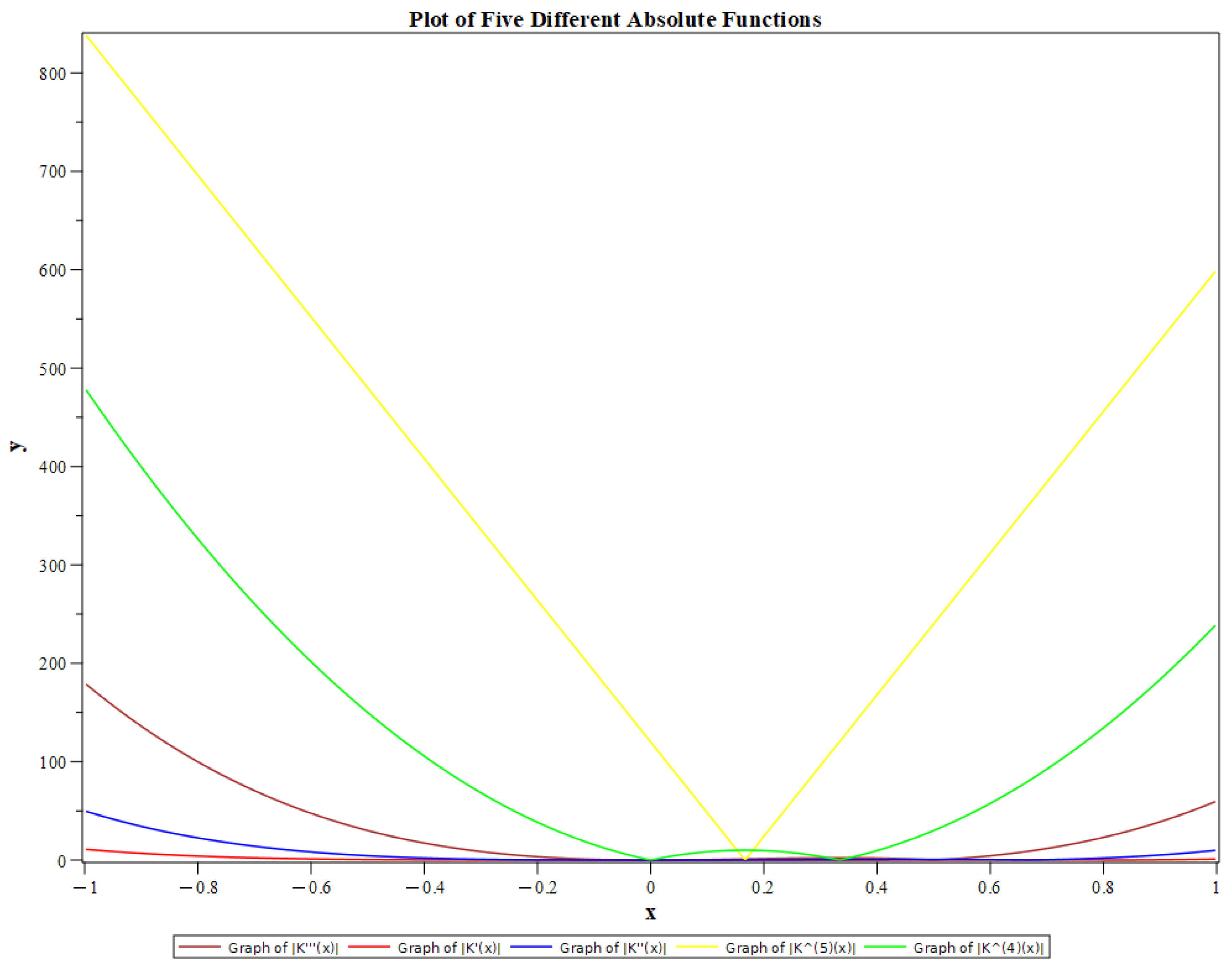
Figure 1. Two-dimensional plot of functions.
Axioms 14 00602 g001
Figure 2. Three-dimensional surface plot of an inequality where blue represents L.H.S and red represents R.H.S.
Axioms 14 00602 g002
Table 1. Comparative analysis of the inequality of Theorem 6 for different values of the parameter a for Example 1.
f ( x ) = e ax Left InequalityRight Inequality
a = 0.5 0.01341 0.01425
a = 0.75 0.03434 0.03755
a = 1 0.06958 0.03755
a = 1.5 0.20413 0.24191
a = 1.75 0.31804 0.38646
a = 2 0.47632 0.73478
Table 2. Comparative analysis of the inequality of Theorem 1 from [22] for different values of the parameter a for Example 1.
f ( x ) = e ax Left InequalityRight Inequality
a = 0.5 0.01341 0.16176
a = 0.75 0.03434 0.27764
a = 1 0.06958 0.42524
a = 1.5 0.20413 0.85146
a = 1.75 0.31804 1.15431
a = 2 0.47632 1.53871
Disclaimer/Publisher’s Note: The statements, opinions and data contained in all publications are solely those of the individual author(s) and contributor(s) and not of MDPI and/or the editor(s). MDPI and/or the editor(s) disclaim responsibility for any injury to people or property resulting from any ideas, methods, instructions or products referred to in the content.