Contour Limits and a “Gliding Hump” Argument

Abstract

We investigate the behavior of solutions of second-order elliptic Dirichlet problems for a convex domain by using a “gliding hump” technique and prove that there are no contour limits at a specified point of the boundary of the domain. Then we consider two-dimensional domains which have a reentrant (i.e., nonconvex) corner at a point P of the boundary of the domain. Assuming certain comparison functions exist, we prove that for any solution of an appropriate Dirichlet problem on the domain whose graph has finite area, there are infinitely many curves of finite length in the domain ending at P along which the solution has a limit at P. We then prove that such behavior occurs for quasilinear operations with positive genre.

1. Introduction

The study of the nonexistence of classical solutions of the Dirichlet problem

$$Qf=0\mathrm{in}\mathrm{\Omega },f=\varphi \mathrm{on}\partial \mathrm{\Omega }$$

(1)

when Q is a second-order elliptic partial differential operator and $\varphi \in C^0(\partial \mathrm{\Omega })$ has a rich history (e.g., [1] (§ 14.4), [2] (§ 406–416), [3,4,5]). When $\varphi$ is discontinuous at $P\in \partial \mathrm{\Omega },$ a classical solution $f\in C^2\left(\mathrm{\Omega }\right)\cap C^0\left(\overline{\mathrm{\Omega }}\right)$ of (1) cannot exist; one example is the helicoid $f(rcos\theta ,rsin\theta )=\theta ,$ which satisfies the two-dimensional Laplace and minimal surface equations in $\mathrm{\Omega }=\left\{\right(rcos\theta ,rsin\theta ):0<r<1,-\alpha <\theta <\alpha \}$ ($\alpha \in (0,\pi )$) and is a generalized (e.g., Perron) solution of the corresponding Dirichlet problems (e.g., [2]). Classical Phragmen–Lindeloff theorems imply that solutions of linear, uniformly elliptic equations which have jump discontinuities at points of the boundary and are bounded or satisfy growth conditions near these points of discontinuity have radial limits at these points (e.g., [6,7]). Solutions of prescribed mean curvature equations with jump discontinuities at points on $\partial \mathrm{\Omega }$ when $\mathrm{\Omega }$ is a domain in ${\mathrm{I}\mathrm{R}}^2$ have radial limits at these points without imposing any growth or boundedness conditions (e.g., [8,9]).

If we eliminate the restriction that $\varphi \in L^{\infty }(\partial \mathrm{\Omega })$ has jump discontinuities at points on $\partial \mathrm{\Omega },$ what can be said about the “contour limits” at $P\in \partial \mathrm{\Omega }$ of a generalized solution of (1)? Here, by “contour limits”, we mean limits along curves (or types of curves) which have P as an endpoint, such as radial limits, tangential limits or nontangential limits. When, for example, $Q=\mathrm{\Delta },$ $\mathrm{\Omega }$ is a unit ball in ${\mathrm{I}\mathrm{R}}^N$ and f is a generalized solution of (1) which has an asymptotic value a at $P\in \partial \mathrm{\Omega },$ we see that a is a contour limit of f at $P;$ thus, asymptotic values can be considered as a special case of contour limits (e.g., [10,11,12]). There are, for example, numerous examples of the existence or nonexistence of different types of contour limits for harmonic functions (e.g., [13,14,15]). For the minimal surface equation on $\mathrm{\Omega }\subset {\mathrm{I}\mathrm{R}}^2,$ there are generalized solutions of (1) for which none of the radial limits exist at a specified point $P\in \partial \mathrm{\Omega }$ ([16]). The construction of such examples can often be characterized as using a “gliding hump technique” (e.g., [17]). Gliding hump techniques work by constructing a sequence (in this case, a sequence of solutions of (1)) with certain properties and by showing that the assumption that the limit of this sequence has a specific property leads to a contradiction. Of course, in these gliding hump examples, the boundary data $\varphi$ is highly oscillatory at P (e.g., like $sin(1/|\mathbf{x}-P\left|\right)$). Some recent articles on the Dirichlet problem allowing highly oscillatory boundary data $\varphi$ or highly oscillatory coefficients $a^{ij}$ (in (4)) are ([18,19]); other recent articles on elliptic boundary value problems involve inverse problems ([20]), capillary hypersurfaces in a wedge ([21]) and the Dirichlet problem of translating mean curvature equations ([22]).

In this study, we first investigate a slight modification of the gliding hump technique used in [16] and consider its application to generalized solutions of (1) when Q is a quasilinear elliptic operator on ${\mathrm{I}\mathrm{R}}^N$ which may not be uniformly elliptic. When $\mathrm{\Omega }$ is convex, we construct examples of generalized solutions $f\in C^2\left(\mathrm{\Omega }\right)\cap C^0\left(\overline{\mathrm{\Omega }}\setminus \left\{P\right\}\right)$ of (1) such that for any curve $\gamma$ in $\overline{\mathrm{\Omega }}$ ending at $P\in \partial \mathrm{\Omega },$ the limit of f at P along $\gamma$ does not exist (see Theorem 1). In the cases under consideration, the structure of the operator and the geometry of the domain play critical roles; in particular, barriers for (1) at a point $P\in \partial \mathrm{\Omega }$ may only exist if $\mathrm{\Omega }$ is locally convex at P (e.g., [1] (Chapter 14)) or mean convex ([23]). Second, we consider domains $\mathrm{\Omega }\subset {\mathrm{I}\mathrm{R}}^2$ which have a nonconvex corner at a point $P\in \partial \mathrm{\Omega }$ and operators Q which have a well-defined genre g (see Definition 3). In 1912, Sergei Bernstein ([24]) expressed the degree of nonlinearity of a quasilinear elliptic partial differential equation through the concept of “genre”, and Jim Serrin extended this concept in their monumental 1969 paper [5]. Using comparison functions from [5,25,26] and assuming that $g>1,$ we shall prove that for any generalized solution $f\in C^2\left(\mathrm{\Omega }\right)\cap C^0\left(\overline{\mathrm{\Omega }}\setminus \left\{P\right\}\right)$ of (1) whose graph has finite area, there exist infinitely many paths $\gamma$ of finite length in $\mathrm{\Omega }$ ending at P such that the limit of f at P along $\gamma$ exists (see Theorem 3). Third, if we assume $\varphi$ has a jump discontinuity at P and Q is an operator with $g>0,$ then we obtain this same conclusion without assuming $\mathrm{\Omega }\subset {\mathrm{I}\mathrm{R}}^2$ has a nonconvex corner at P (see Theorem 4).

The significance of this work is its examination of the question “How might a bounded generalized solution of (1) behave at (or near) a point $P\in \partial \mathrm{\Omega }$ when $\varphi \in L^{\infty }(\partial \mathrm{\Omega })$ is discontinuous at P?” as well as its illustration of the importance of the geometry of $\mathrm{\Omega }$ (i.e., do local barriers for (1) exist at and near P), the genre of Q and the type of discontinuity of $\varphi$ at $P.$ One question of interest is “Does there exist a connection between the existence of radial limits of f at P and the existence of any contour limit of f at P?” Is there any way of constructing a bounded generalized solution f of (1) which does not have radial limits at P and is fundamentally different than that in Section 2?

2. The Gliding Hump Construction

Let $N\ge 2$ and $\mathrm{\Omega }\subset {\mathrm{I}\mathrm{R}}^N$ be a bounded, open, locally Lipschitz domain. Consider the Dirichlet problem

$$\begin{array}{ccc}\hfill Qf& =& 0\mathrm{in}\mathrm{\Omega },\hfill \end{array}$$

(2)

$$\begin{array}{ccc}\hfill f& =& \varphi \mathrm{on}\partial \mathrm{\Omega },\hfill \end{array}$$

(3)

where Q is a quasilinear elliptic operator on $C^2\left(\mathrm{\Omega }\right)$ given by

$$Qf=\sum _{i,j=1}^N{a}^{ij}(·, f, Df)D_{ij}f\mathrm{with}{a}^{ij}=a^{ji},1\le i,j\le N,$$

(4)

for $f\in C^2\left(\mathrm{\Omega }\right)$ and $\varphi \in L^{\infty }(\partial \mathrm{\Omega }).$ When there is a neighborhood $U=U\left(\mathbf{x}\right)$ of each point $\mathbf{x}\in \partial \mathrm{\Omega }\setminus \left\{P\right\}$ such that $P\notin \overline{U}$ and $\mathrm{\Omega }\cap U$ is convex, local barriers for (2) and (3) exist in $U\left(\mathbf{x}\right)$ (e.g., [1] (Chapter 14)) in $U\left(\mathbf{x}\right),$ for each $\mathbf{x}\in \partial \mathrm{\Omega }\setminus \left\{P\right\}$ (as might happen when $\varphi$ is smooth on $\partial \mathrm{\Omega }\setminus \left\{P\right\}$), and therefore, the generalized (e.g., Perron) solution f of (2) and (3) will satisfy $f=\varphi$ on $\partial \mathrm{\Omega }\setminus \left\{P\right\},$ even if $\varphi$ is highly oscillatory at P (so that $\varphi$ does not have a one-sided limit from either side of P when $\mathrm{\Omega }\subset {\mathrm{I}\mathrm{R}}^2).$

Let us suppose that the following two assumptions hold for $Q.$

Assumption 1

(Compactness Principle). Let $\left\{f_n\right\}$ be a uniformly bounded sequence of solutions of (2) in a domain $\mathrm{\Omega }\subset {\mathrm{I}\mathrm{R}}^N.$ Then there exists a subsequence which converges to a solution of (2) in $\mathrm{\Omega },$ the convergence being uniform on every compact subset of $\mathrm{\Omega }.$

Assumption 2

(Localization Lemma). Let $\mathrm{\Omega }\subset {\mathrm{I}\mathrm{R}}^N$ be an open convex set with $P\in \partial \mathrm{\Omega }.$ Let $ϵ>0$ and $h\in C^2\left(\mathrm{\Omega }\right)\cap C^0(\mathrm{\Omega }\cup \left\{P\right\})$ be a solution of (2) in Ω with $\left|h\right|\le 2.$ Then for each $\delta >0,$ there exists a solution $g\in C^2\left(\mathrm{\Omega }\right)\cap C^0(\mathrm{\Omega }\cup \left\{P\right\})$ of (2) in Ω such that $g\left(P\right)=2,$ $\left|g\right|\le 2,$ and $sup\left\{\right|g\left(\mathbf{x}\right)-h\left(\mathbf{x}\right)|:\mathbf{x}\in \mathrm{\Omega },\mathrm{dist}(\mathbf{x},\partial \mathrm{\Omega })\ge \delta \}<ϵ.$

Remark 1.

The validity of these assumptions follows when interior a priori gradient estimates exist. The proof of the Compactness Principle follows from a priori gradient estimates and a uniform bound on the magnitude of f when Q is the two-dimensional minimal surface equation ([27] (p. 323)). The Monotone Convergence Theorem ([27] (p. 329)), which is used in the proof of the Localization Lemma for minimal surfaces ([16] (Lemma)), relies on an a priori estimate of the gradient of nonnegative solutions (e.g., footnote 4 of [27] (p. 329)). Such a priori gradient estimates occur in certain classes of elliptic equations (e.g., [28,29,30,31,32], [1] (Theorem 15.3 and Theorem 16.21)). However, the following comment in 1969 by Serrin ([5] (p. 492)) illustrates the difficulty in obtaining such a priori estimates: “That the result stated there” (in [24]) “cannot be correct follows from an example of Finn (1954, page 399). The problem is of course that of obtaining interior estimates for the gradient of a solution in terms of a maximum bound, but independent of the particular boundary data”.

Theorem 1.

Suppose Assumptions 1 and 2 hold for $Q.$ Let $\mathrm{\Omega }\subset {\mathrm{I}\mathrm{R}}^N$ be an open convex set with $P\in \partial \mathrm{\Omega }$ and let $B\left(r\right)=\{\mathbf{x}\in {\mathrm{I}\mathrm{R}}^N:|\mathbf{x}-P|<r\}.$ There exists $f\in C^2\left(\mathrm{\Omega }\right)$ satisfying $Qf=0$ in Ω with $\left|f\right|\le 2,$ $f\ge 1$ on $\partial B\left(r_{2n}\right)\cap \overline{\mathrm{\Omega }}$ and $f\le -1$ on $\partial B\left(r_{2n+1}\right)\cap \overline{\mathrm{\Omega }}$ for each $n\in \mathrm{I}\mathrm{N},$ where $B\left(r\right)\stackrel{\mathsf{def}}{=}\{\mathbf{x}\in \mathrm{\Omega }:|\mathbf{x}-P|<r\}$ and $\left\{r_n\right\}$ is a decreasing sequence in $(0,1)$ with ${lim}_{n\to \infty }{r}_n=0,$ and constructed using a (modified) gliding hump technique. There is no path γ in Ω from an interior point of Ω to P along which f has a limit at $P.$

Proof. 

Let ${\mathrm{\Omega }}_0\subset {\mathrm{I}\mathrm{R}}^N$ be an open convex set such that ${\mathrm{\Omega }}_0\cap \overline{\mathrm{\Omega }}=\mathrm{\Omega }\cup \left\{P\right\}.$ Let $f_1\in C^2\left({\mathrm{\Omega }}_0\right)\cap C^0\left(\overline{{\mathrm{\Omega }}_0}\right)$ satisfy (2) in ${\mathrm{\Omega }}_0$ such that $|f_1|\le 2$ and $f_1(0,0)=-2.$ Since $f_1\in C^0\left(\overline{{\mathrm{\Omega }}_0}\right),$ there exists $r_1\in (0,1)$ such that $f_1\left(\mathbf{x}\right)<-1$ for $\mathbf{x}\in B\left(r_1\right)\cap {\mathrm{\Omega }}_0.$ Set ${ϵ}_1=-(1+inf\{f_1\left(\mathbf{x}\right):\mathbf{x}\in \partial B\left(r_1\right)\cap \overline{\mathrm{\Omega }}\})>0.$ From Assumption 2, we see that there exists $f_2\in C^2\left({\mathrm{\Omega }}_0\right)\cap C^0({\mathrm{\Omega }}_0\cup \left\{P\right\})$, which satisfies (2) in ${\mathrm{\Omega }}_0$ such that $|f_2|\le 2,$ $f_2\left(P\right)=2,$ and $sup\left\{\right|f_2\left(\mathbf{x}\right)-f_1\left(\mathbf{x}\right)|:\mathbf{x}\in {\mathrm{\Omega }}_0,\mathrm{dist}(\mathbf{x},\partial {\mathrm{\Omega }}_0)\ge {\delta }_1\}<{ϵ}_1,$ where ${\delta }_1=\mathrm{dist}(\partial B\left(r_1\right)\cap \overline{\mathrm{\Omega }},\partial {\mathrm{\Omega }}_0).$ Notice that $f_2\left(\mathbf{x}\right)>1$ for each $\mathbf{x}\in \partial B\left(r_1\right)\cap \overline{\mathrm{\Omega }}.$

We shall construct our “gliding hump” sequence. Let us suppose $\{f_k:1\le k\le n\}$ have been defined. Set ${\delta }_n=\mathrm{dist}(\partial B\left(r_n\right)\cap \overline{\mathrm{\Omega }},\partial {\mathrm{\Omega }}_0)$ and

$${ϵ}_n=\underset{1\le k\le n}{min}\{inf\{|f_n\left(\mathbf{x}\right)-{(-1)}^k|:\mathbf{x}\in \partial B\left(r_k\right)\cap \overline{\mathrm{\Omega }}\left\}\right\}.$$

Then Assumption 1 implies that there exists $f_{n+1}\in C^2\left({\mathrm{\Omega }}_0\right)\cap C^0({\mathrm{\Omega }}_0\cup \left\{P\right\})$, which satisfies (2) in ${\mathrm{\Omega }}_0$ such that $f_{n+1}\left(P\right)=2{(-1)}^{n+1},$ $|f_{n+1}|\le 2,$ and $sup\left\{\right|f_{n+1}\left(\mathbf{x}\right)-f_n\left(\mathbf{x}\right)|:\mathbf{x}\in {\mathrm{\Omega }}_0,\mathrm{dist}(\mathbf{x},\partial {\mathrm{\Omega }}_0)\ge {\delta }_n\}<{ϵ}_n.$ Since ${(-1)}^{n+1}{f}_{n+1}\left(P\right)=2$ and $f_{n+1}\in C^0({\mathrm{\Omega }}_0\cup \left\{P\right\}),$ there exists $r_{n+1}\in (0,r_n)$ with $r_{n+1}<1/(n+1)$ such that

$${(-1)}^{n+1}{f}_{n+1}\left(\mathbf{x}\right)>1\mathrm{for}\mathbf{x}\in B\left(r_{n+1}\right)\cap {\mathrm{\Omega }}_0;$$

in particular, ${(-1)}^{n+1}{f}_{n+1}\left(\mathbf{x}\right)>1$ for each $\mathbf{x}\in \partial B\left(r_{n+1}\right)\cap \overline{\mathrm{\Omega }}.$

For each $r>0,$ consider the compact subsets $K_r=\overline{\mathrm{\Omega }}\setminus B\left(r\right)$ of ${\mathrm{\Omega }}_0.$ The sequence $\left\{f_n\right\}$ is uniformly bounded and so Assumption 1 implies that a subsequence of $\left\{f_n\right\},$ still denoted $\left\{f_n\right\},$ converges uniformly on compacta in ${\mathrm{\Omega }}_0$ to a solution f of (2) in ${\mathrm{\Omega }}_0$ such that $\left|f\right|\le 2.$ Notice that for each $r>0,$ $\left\{f_n\right\}$ converges uniformly on $K_r$ to f and so ${(-1)}^{n}f\left(\mathbf{x}\right)\ge 1$ when $\mathbf{x}\in \partial B\left(r_n\right)\cap \overline{\mathrm{\Omega }}$ for $n\in \mathrm{I}\mathrm{N}.$ Thus, f has an infinite number of “ridges” (i.e., $\partial B\left(r_{2n}\right)\cap \overline{\mathrm{\Omega }}$ (where $f\ge 1$) for each $n\in \mathrm{I}\mathrm{N}$) and “troughs” (i.e., $\partial B\left(r_{2n+1}\right)\cap \overline{\mathrm{\Omega }}$ (where $f\le -1$) for each $n\in \mathrm{I}\mathrm{N}$) converging to $\left\{P\right\}.$ In particular, there is no path $\gamma$ in $\mathrm{\Omega }$ from an interior point of $\mathrm{\Omega }$ to $(0,0)$ along which f has a limit at $(0,0).$ □

Remark 2.

When Ω is the unit ball in ${\mathrm{I}\mathrm{R}}^N,$ $P\in \partial \mathrm{\Omega }$ and $Q=\mathrm{\Delta },$ one might characterize the conclusion of Theorem 1 as follows: There exists $f\in C^2\left(\mathrm{\Omega }\right)$ satisfying $Qf=0$ in Ω with $\left|f\right|\le 2$ such that f has no asymptotic value at P but every value in $[-1,1]$ is a limit value of f at P in the sense that for each $t\in [-1,1],$ there is a sequence $\left\{{\mathbf{x}}_n\right\}$ in Ω converging to P and $f(x_n,y_n)=t$ for each $n\in \mathrm{I}\mathrm{N}.$

3. Nonconvex Corners

The existence of the radial limits at $P\in \partial \mathrm{\Omega }$ of $f\in C^2\left(\mathrm{\Omega }\right)\cap C^0(\overline{\mathrm{\Omega }}\setminus \left\{P\right\})$ when $\mathrm{\Omega }$ is a locally Lipschitz open set in ${\mathrm{I}\mathrm{R}}^2$ and f is a solution of a prescribed mean curvature equation (with mean curvature H) for various choices of H (and Dirichlet or contact angle boundary conditions) was first established by the second author for $H\equiv 0$ (e.g., [2] (§ 416)) and extended to general H in [8] (see also [33,34]). These results assume the boundary data satisfies certain conditions; for example, in Dirichlet problems, the prescribed boundary data $\varphi$ have, at worst, a jump discontinuity at $P.$ The proofs of these results follow the pattern in [8] of proving that a conformal parameterization of the graph of f is continuous on the closure of the parameter domain and using [35] to establish the Hölder continuity on $E\cup \mathrm{\Sigma }$ of the first derivative of the parameterization (for an appropriate $\mathrm{\Sigma }\subset \partial E$) and then prove that the radial limits exist.

An initial part of the proofs above consists of the following argument. Suppose that $f\in C^2\left(\mathrm{\Omega }\right)\cap L^{\infty }\left(\mathrm{\Omega }\right)$ and $\mathcal{S}\stackrel{\mathsf{def}}{=}\left\{\right(\mathbf{x},f\left(\mathbf{x}\right)):\mathbf{x}\in \mathrm{\Omega }\}$ has finite area $A\left(\mathcal{S}\right).$ For our purposes, we may assume $\mathrm{\Omega }$ is a simply connected set. Let $Y\in C^2(E:{\mathrm{I}\mathrm{R}}^3)$ be an isothermal (i.e., conformal) parameterization of $\mathcal{S},$ so that $Y\left(E\right)=\mathcal{S},$ where $E=\{\mathbf{u}\in {\mathrm{I}\mathrm{R}}^2:|\mathbf{u}|<1\}.$ For ${\mathbf{u}}_{\mathbf{0}}=(u_0,v_0)\in \partial E,$ let $B_r=B_r\left({\mathbf{u}}_{\mathbf{0}}\right)=\{\mathbf{u}\in \overline{E}:|\mathbf{u}-{\mathbf{u}}_{\mathbf{0}}|<r\},$ $C_r=C_r\left({\mathbf{u}}_{\mathbf{0}}\right)=\{\mathbf{u}\in \overline{E}:|\mathbf{u}-{\mathbf{u}}_{\mathbf{0}}|=r\},$ and $l_r$ be the length of the image curve $Y\left(C_r\right).$ The Courant–Lebesgue Lemma asserts that for each $\delta >0,$ there exists a number $\rho \left(\delta \right)\in (\delta ,\sqrt{\delta })$ so that $l_{\rho \left(\delta \right)}<p\left(\delta \right),$ where $p\left(t\right)=\sqrt{8\pi A\left(\mathcal{S}\right)/ln(1/t)},$ $0<t<1.$

The “Fundamental Lemma” ([36] (Lemma 3.1)) used above plays a critical role:

Lemma 1

(Courant–Lebesgue Lemma). In a domain B of the $uv$—plane, consider the class of piecewise smooth vectors X for which the Dirichlet integral is uniformly bounded by a constant $M:$

$$D\left[X\right]\stackrel{\mathsf{def}}{=}{\displaystyle \frac{1}{2}}{\int }_B\left(X_u·X_u+X_v·X_v\right)dudv\le M.$$

About an arbitrary fixed point O, we draw circles of radius $r.$ Denote by $C_r$ an arc or set of arcs of such a circle contained in $B,$ by s arclength on $C_r.$ Then for every positive $\delta <1$ there exists a value $\rho ,$ depending on $X,$ with $\delta \le \rho \le \sqrt{\delta },$ such that

$${\int }_{C_r}{X}_s^{2}ds\le {\displaystyle \frac{ϵ\left(\delta \right)}{\rho }}\mathrm{with}ϵ\left(\delta \right)={\displaystyle \frac{4M}{log\left(\frac{1}{\delta }\right)}}$$

tending to zero for $\delta \to 0.$ Furthermore, the square of the length $L_{\rho }$ of the image $C_{\rho }^{\prime }$ of $C_{\rho }$ in $x,y,z$—space has the bound $L_{\rho }^2\le 2\pi ϵ\left(\delta \right),$ i.e., the oscillation of $X(u,v)$ on $C_{\rho }$ is at most $\sqrt{2\pi ϵ\left(\delta \right)}.$

Recall that $D\left[X\right]\ge A\left(X\right),$ where $A\left(X\right)$ is the surface area of the image $X\left(B\right)$ of $B,$ and $D\left[X\right]=A\left(X\right)$ if the surface $X\left(B\right)$ is represented in conformal (i.e., isothermal or isometric) coordinates ([36] (§ 3.1)).

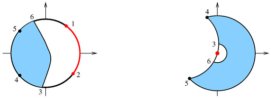
In [9], the proofs above (of, for example, [8]) are modified to prove that if $\mathrm{\Omega }$ has a “reentrant” (i.e., nonconvex) corner at $P=(0,0)\in \partial \mathrm{\Omega }$ (e.g., Figure 1), then the nontangential radial limits at P of f exist without regard to the restrictions on the boundary data noted above. To see that the conformal parameterization of the graph of f is continuous on the closure of the parameter domain, one uses the Courant–Lebesgue Lemma as noted and particular comparison functions, specifically catenoids for $H\equiv 0$ and unduloids for $H\in L^{\infty }\left(\mathrm{\Omega }\right),$ to control the oscillation of the third component of Y and prove that Y is uniformly continuous on $E.$ This topic was investigated further, illustrated in [37] (Example 1.4) (see also [38]) (p. 430) when Q is the minimal surface operator on ${\mathrm{I}\mathrm{R}}^2,$ $\mathrm{\Omega }=\{(x,y)\in {\mathrm{I}\mathrm{R}}^2:1<{(x+1)}^2+y^2<{cosh}^2\left(1\right)\},$ $P=(0,0)\in \partial \mathrm{\Omega },$ $\varphi \left(\mathbf{x}\right)={sin(\pi /|\mathbf{x}|}^2)\in C^0(\overline{\mathrm{\Omega }}\setminus \left\{P\right\})$ and $f\in C^0\left(\overline{\mathrm{\Omega }}\right)$ (see Figure 2). In this case, $\mathrm{\Omega }$ is not locally convex at any point of the inner boundary $T=\{(x,y)\in {\mathrm{I}\mathrm{R}}^2:{(x+1)}^2+y^2=1\}$ of $\mathrm{\Omega }$ and f need not equal $\varphi$ on $T.$ Standard results (e.g., [38] (Theorem 3)) show that $f\in C^0(\overline{\mathrm{\Omega }}\setminus \left\{P\right\}).$ To see that Y is continuous on the closure of the parameter domain, one works in a neighborhood U of P and uses “Bernstein functions” ([37] (Lemma 2.3)) to control the oscillation of the third component of the conformal parameterization of the graph of f restricted to $U\cap \mathrm{\Omega }$ (a catenoid would have worked just as well for this particular example). The continuity of f at P then follows from the symmetry of the problem.

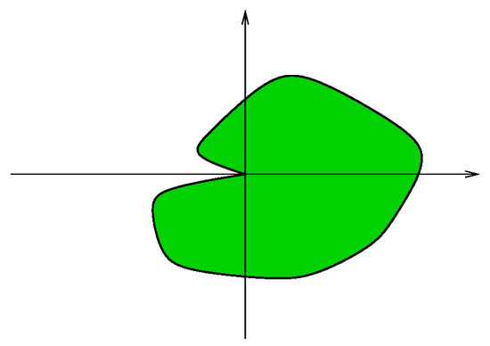
Figure 1. A domain $\mathrm{\Omega }$ with a reentrant corner at $(0,0)$.

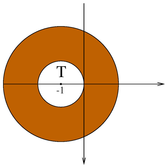
Figure 2. $\mathrm{\Omega }$.

A brief discussion of the use of catenoids and unduloids as comparison functions in [9] may help illustrate the use of comparison functions in Theorems 2 and 3. In [9], nothing (except boundedness) is known about the behavior of f (or $\varphi$) on $\partial \mathrm{\Omega }$, and it is necessary to avoid $\partial \mathrm{\Omega }\setminus \left\{P\right\}.$ Thus, we restrict our attention to a subdomain ${\mathrm{\Omega }}_1$ of $\mathrm{\Omega }$ such as those illustrated in Figure 3 (right) and Figure 4 (right). If $Y:E\to {\mathrm{I}\mathrm{R}}^3$ is the isothermal parameterization of the graph of f over ${\mathrm{\Omega }}_1$ with $Y(u,v)=\left(x\right(u,v),y(u,v),z(u,v\left)\right)$ and $z(u,v)=f\left(x\right(u,v),y(u,v\left)\right),$ then the oscillation of z on the curves $C_r,$ labeled a through g in Figure 4 (left), is controlled by the Courant–Lebesgue Lemma. If m and M are the infimum and supremum of z on $C_r,$ then [1] (Theorem 14.10) implies $m+h_P^{-}\le z\le M+h_P^{+}$ in the region $B_r$ between $C_r$ and $\partial E,$ where the graphs of $h_P^{\pm }$ are appropriate catenoids in [9]. Since we have uniform control of $M+h_P^{+}-m-h_P^{-}$ in $B_r,$ we see that z and Y are uniformly continuous on $E.$

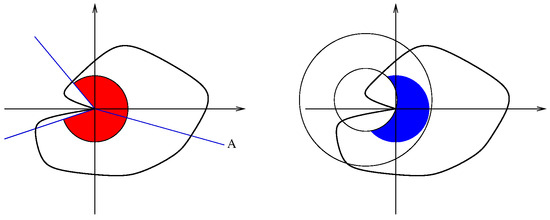
Figure 3. $D_{\alpha }\left(\lambda \right)$ in $\mathrm{\Omega }$ ($A=(cos{\theta }_0,sin{\theta }_0)$); ${\mathrm{\Omega }}_1=D_{\alpha }\left(\lambda \right)\cap {\mathcal{A}}_{{\mathbf{x}}_0}$.

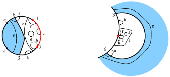
Figure 4. Examples of circular arcs $C_r$ and $G\left(C_r\right)$.

Assuming that the use of catenoids or unduloids as comparison functions could be replaced by different comparison functions for (2) (e.g., [37]), this argument depends solely on the assumption that the area of the graph of the solution of (2) is finite. So suppose that there exist numbers $0<r_1<r_2$ and functions $h^{\pm }\in C^2\left(\mathcal{A}\right)\cap C^0\left(\overline{\mathcal{A}}\right)$ such that the graph of $h^{+}$ makes a contact angle of zero with the cylinder $\partial {\mathcal{A}}_1\times \mathrm{I}\mathrm{R},$ and the graph of $h^{-}$ makes a contact angle of $\pi$ with the cylinder $\partial {\mathcal{A}}_1\times \mathrm{I}\mathrm{R},$ where $\mathcal{A}=\{\mathbf{x}\in {\mathrm{I}\mathrm{R}}^2:r_1<|\mathbf{x}|<r_2\}$ and $\partial {\mathcal{A}}_k=\{\mathbf{x}\in {\mathrm{I}\mathrm{R}}^2:\left|\mathbf{x}\right|=r_k\},$ $k=1,2.$ Suppose further that

$$Q{h}_{{\mathbf{x}}_{\mathbf{0}}}^{+}\left(\mathbf{x}\right)\le 0\mathrm{and}Q{h}_{{\mathbf{x}}_{\mathbf{0}}}^{-}\left(\mathbf{x}\right)\ge 0$$

(5)

for ${\mathbf{x}}_{\mathbf{0}}\in {\mathrm{I}\mathrm{R}}^2,$ $\mathbf{x}\in \mathrm{\Omega }\cap \overline{{\mathcal{A}}_{{\mathbf{x}}_{\mathbf{0}}}}$ and $c\in [-J,J]$ for $J>0,$ where ${\mathcal{A}}_{{\mathbf{x}}_{\mathbf{0}}}=\{\mathbf{x}\in {\mathrm{I}\mathrm{R}}^2:\mathbf{x}-{\mathbf{x}}_{\mathbf{0}}\in \mathcal{A}\}$ and $h_{{\mathbf{x}}_{\mathbf{0}}}^{\pm }\left(\mathbf{x}\right)=h^{\pm }(\mathbf{x}-{\mathbf{x}}_{\mathbf{0}})$ for $\mathbf{x}\in \overline{{\mathcal{A}}_{{\mathbf{x}}_{\mathbf{0}}}}.$ These functions $h^{\pm }$ are “Bernstein (comparison) functions” and they are necessary to prove the existence of contour limits (see Remark 4); they will play a critical role in the remainder of this article (see [1] (p. 357) for a brief discussion of such comparison functions).

In contrast to Theorem 1, we claim the following:

Theorem 2.

Suppose $\mathrm{\Omega }\subset {\mathrm{I}\mathrm{R}}^2$ is an open set, $P\in \partial \mathrm{\Omega }$ and there exist $\alpha \in \left(\pi /2,\pi \right),$ $\lambda >0$ and ${\theta }_0\in [0,2\pi )$ such that $\overline{D_{\alpha }\left(\lambda \right)}\subset \mathrm{\Omega }\cup \left\{P\right\},$ where $D_{\alpha }\left(\lambda \right)=\{P+(rcos\theta ,rsin\theta ):0<r<\lambda ,-\alpha <\theta -{\theta }_0<\alpha \}$ (see Figure 3 (left)). Suppose there exist comparison functions $h^{\pm }$ for (2) as described above. Let $f\in C^2\left(\mathrm{\Omega }\right)\cap L^{\infty }\left(\mathrm{\Omega }\right)$ satisfy (2) such that the area of the graph of f is finite. Then there exist (infinitely many) paths γ of finite length in Ω ending at P along which f has a limit at $P.$

Proof. 

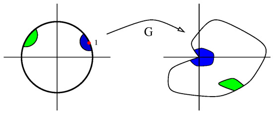
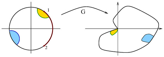
We may assume $P=(0,0)$ and $\lambda <r_2-r_1.$ Set $\mathcal{S}=\left\{\right(\mathbf{x},f\left(\mathbf{x}\right)):\mathbf{x}\in \mathrm{\Omega }\}$ and let $A\left(\mathcal{S}\right)<\infty$ be the area of $\mathcal{S}.$ Choose ${\mathbf{x}}_0\in {\mathrm{I}\mathrm{R}}^2$ such that ${\mathbf{x}}_0-P=r_1(cos{\theta }_1,sin{\theta }_1)$ and set ${\mathrm{\Omega }}_1=D_{\alpha }\left(\lambda \right)\cap {\mathcal{A}}_{{\mathbf{x}}_0},$ for some ${\theta }_1\in ({\theta }_0-\alpha +\pi /2,{\theta }_0+\alpha +3\pi /2)$ (see Figure 3 (right)). Let ${\mathcal{S}}_1=\{(\mathbf{x},f\left(\mathbf{x}\right)):\mathbf{x}\in {\mathrm{\Omega }}_1\};$ then the area $A\left({\mathcal{S}}_1\right)$ of ${\mathcal{S}}_1$ satisfies $A\left({\mathcal{S}}_1\right)<A\left(\mathcal{S}\right)<\infty .$ Now $\partial {\mathrm{\Omega }}_1\setminus \left\{P\right\}$ consists of three pieces, which are ${\partial }^{+}{D}_{\alpha }\left(\lambda \right)=\{P+(\lambda cos\theta ,\lambda sin\theta ):-\alpha \le \theta -{\theta }_0\le \alpha \}$ and the two components of ${\partial }^{+}{\mathcal{A}}_{{\mathbf{x}}_0}=\{\mathbf{x}\in {\mathrm{\Omega }}_1:|\mathbf{x}-{\mathbf{x}}_{\mathbf{0}}|=r_1\};$ notice that $P\notin {\mathrm{\Omega }}_1$ and so $P\notin {\partial }^{+}{\mathcal{A}}_{{\mathbf{x}}_0}.$

There exists an isothermal (conformal) parameterization $Y:E\to {\mathrm{I}\mathrm{R}}^3$ of ${\mathcal{S}}_1;$ that is, Y is a diffeomorphism of E and ${\mathcal{S}}_1,$ $Y_u·Y_v=0$ on $E,$ $|Y_u| = |Y_v|$ on $E,$ $Y\left(E\right)={\mathcal{S}}_1$ and $D\left(Y\right)=A\left({\mathcal{S}}_1\right),$ where $D\left(Y\right)={\int }_E\left(\right|Y_u{|}^2+|Y_v{|}^2)dudv$ is the Dirichlet integral of $Y.$ Let us write $Y(u,v)=\left(x\right(u,v),y(u,v),z(u,v\left)\right)$ and set $G(u,v)=\left(x\right(u,v),y(u,v\left)\right)$ for $(u,v)\in E,$ so $z=f\circ G$ on E and $D\left(G\right)\le D\left(Y\right)\le A\left(\mathcal{S}\right)<\infty .$ Then G extends to a function in $C^0\left(\overline{E}\right),$ $G\left(\overline{E}\right)=\overline{{\mathrm{\Omega }}_1},$ G is a diffeomorphism of E and ${\mathrm{\Omega }}_1,$ the preimage under G of $\partial {\mathrm{\Omega }}_1\setminus \left\{P\right\}$ is an open, connected arc $\sigma$ of $\partial E$ and G is a homeomorphism of $E\cup \sigma$ and $\overline{{\mathrm{\Omega }}_1}\setminus \left\{P\right\}$ (see the proof of [8] (Lemma 2.1)).

We claim that Y is uniformly continuous on E and so extends to a function $Y\in C^0\left(\overline{E}\right).$ This only requires that we prove that the third component $z(·)$ of Y is uniformly continuous on $E.$ We shall let $\mathcal{M}$ denote the set of continuous, strictly increasing functions from the nonnegative reals to the nonnegative reals which are zero at zero; moduli of continuity will be chosen in this class.

Set $E_1=E\setminus G^{-1}\left(D_{\alpha }(\lambda /4)\right)=G^{-1}\left({\mathrm{\Omega }}_1\setminus D_{\alpha }(\lambda /4)\right)$ (see Figure 5, where $\omega =\partial E\setminus \sigma$ is the (shorter) arc joining points labeled 1 and 2). Now $f\in C^2\left(\overline{{\mathrm{\Omega }}_1\setminus D_{\alpha }(\lambda /4)}\right);$ hence $z(·)\in C^0\left(\overline{E_1}\right)$, and so there exists $q_1\in \mathcal{M}$ such that $|z\left({\mathbf{u}}_2\right)-z\left({\mathbf{u}}_1\right)|\le q_1\left(\right|{\mathbf{u}}_2-{\mathbf{u}}_1\left|\right)$ when ${\mathbf{u}}_1,{\mathbf{u}}_2\in \overline{E_1}.$ Since $h^{\pm }\in C^0\left(\overline{\mathcal{A}}\right),$ for each $\epsilon >0,$ there exists $q_2\in \mathcal{M}$ such that $|h^{\pm }\left({\mathbf{x}}_2\right)-h^{\pm }\left({\mathbf{x}}_1\right)|<q_2\left(\right|{\mathbf{x}}_2-{\mathbf{x}}_1\left|\right)$ whenever ${\mathbf{x}}_1,{\mathbf{x}}_2\in \overline{\mathcal{A}}.$

Figure 5. $E_1$ (left), ${\mathrm{\Omega }}_1\setminus D_{\alpha }(\lambda /4)$ (right).

For ${\mathbf{u}}_0\in E,$ let $B_r=B_r\left({\mathbf{u}}_0\right)=\{\mathbf{u}\in E:|\mathbf{u}-{\mathbf{u}}_0|<r\},$ $C_r=C_r\left({\mathbf{u}}_0\right)=\{\mathbf{u}\in E:|\mathbf{u}-{\mathbf{u}}_0|=r\},$ $E_r\left({\mathbf{u}}_0\right)=\partial B_r\left({\mathbf{u}}_0\right)\setminus C_r\left(\mathbf{u}\right)$ and $l_r\left({\mathbf{u}}_0\right)$ be the length of the image curve $Y\left(C_r\left({\mathbf{u}}_0\right)\right)$ as before. Let $m_r\left({\mathbf{u}}_{\mathbf{0}}\right)={inf}_{\mathbf{u}\in C_r\left({\mathbf{u}}_{\mathbf{0}}\right)}z\left(\mathbf{u}\right)={inf}_{\mathbf{x}\in G\left(C_r\left({\mathbf{u}}_{\mathbf{0}}\right)\right)}f\left(\mathbf{x}\right)$ and $M_r\left({\mathbf{u}}_{\mathbf{0}}\right)={sup}_{\mathbf{u}\in C_r\left({\mathbf{u}}_{\mathbf{0}}\right)}z\left(\mathbf{u}\right)={sup}_{\mathbf{x}\in G\left(C_r\left({\mathbf{u}}_{\mathbf{0}}\right)\right)}f\left(\mathbf{x}\right).$ Let $M_r^{-}\left(G\left({\mathbf{u}}_0\right)\right)={sup}_{\mathbf{x}\in G\left(C_r\left({\mathbf{u}}_0\right)\right)}{h}_{{\mathbf{x}}_0}^{-}\left(\mathbf{x}\right)$ and $m_r^{+}={inf}_{\mathbf{x}\in G\left(C_r\left({\mathbf{u}}_{\mathbf{0}}\right)\right)}{h}_{{\mathbf{x}}_0}^{+}\left(\mathbf{x}\right);$ then $h_{{\mathbf{x}}_0}^{-}\left(\mathbf{x}\right)-M_r^{-}\left(G\left({\mathbf{u}}_0\right)\right)\le 0$ on $G\left(C_r\left({\mathbf{u}}_0\right)\right)$ and $h_{{\mathbf{x}}_0}^{+}\left(\mathbf{x}\right)-m_r^{+}\left(G\left({\mathbf{u}}_0\right)\right)\ge 0$ on $G\left(C_r\left({\mathbf{u}}_0\right)\right).$ Further $|h_{{\mathbf{x}}_0}^{-}\left(\mathbf{x}\right)-M_r^{-}\left(G\left({\mathbf{u}}_0\right)\right)|\le q_2\left(l_r\left({\mathbf{u}}_0\right)\right)$ and $|h_{{\mathbf{x}}_0}^{+}\left(\mathbf{x}\right)-m_r^{+}\left(G\left({\mathbf{u}}_0\right)\right)|\le q_2\left(l_r\left({\mathbf{u}}_0\right)\right)$ for $\mathbf{x}\in G\left(C_r\left({\mathbf{u}}_0\right)\right).$

Let $ϵ>0.$ Choose $\delta \in (0,1)$ such that $p\left(\delta \right)<min\{ϵ/3,\lambda /4,q_2^{-1}(ϵ/3)\}$ and $2\sqrt{\delta }<q_1^{-1}\left(ϵ\right).$ Let ${\mathbf{u}}_{\mathbf{0}}\in E.$ From the Courant–Lebesgue Lemma, there exists $\rho =\rho (\delta ,{\mathbf{u}}_{\mathbf{0}})\in (\delta ,\sqrt{\delta })$ such that $l_{\rho }(\delta ,{\mathbf{u}}_{\mathbf{0}})<p\left(\delta \right).$ There are two possibilities: (i) $\overline{B_{\rho \left(\delta ,{\mathbf{u}}_{\mathbf{0}}\right)}\left({\mathbf{u}}_{\mathbf{0}}\right)}\cap (E\setminus E_1)=\varnothing$ and (ii) $\overline{B_{\rho (\delta ,{\mathbf{u}}_{\mathbf{0}})}\left({\mathbf{u}}_{\mathbf{0}}\right)}\cap (E\setminus E_1)\ne \varnothing .$ Consider case (i) first. Then $\overline{B_{\rho (\delta ,{\mathbf{u}}_{\mathbf{0}})}\left({\mathbf{u}}_{\mathbf{0}}\right)}\cap E\subset E_1$ and so, for ${\mathbf{u}}_1,{\mathbf{u}}_2\in \overline{B_{\rho (\delta ,{\mathbf{u}}_{\mathbf{0}})}\left({\mathbf{u}}_{\mathbf{0}}\right)}\cap E,$

$$|z\left({\mathbf{u}}_2\right)-z\left({\mathbf{u}}_1\right)|\le q_1\left(\right|{\mathbf{u}}_2-{\mathbf{u}}_1\left|\right)\le q_1\left(2\rho (\delta ,{\mathbf{u}}_{\mathbf{0}})\right))\le q_1\left(2\sqrt{\delta }\right)<ϵ.$$

Now we consider case (ii). Let $\mathbf{u}\in \overline{B_{\rho (\delta ,{\mathbf{u}}_{\mathbf{0}})}\left({\mathbf{u}}_{\mathbf{0}}\right)}\cap E$ ($\mathbf{u}$ may not be in $E\setminus E_1$) and set $\mathbf{x}=G\left(\mathbf{u}\right).$ Then there exists a point ${\mathbf{u}}_3\in C_{\rho (\delta ,{\mathbf{u}}_{\mathbf{0}})}\left({\mathbf{u}}_{\mathbf{0}}\right)\cap (E\setminus E_1).$ Setting ${\mathbf{x}}_3=G\left({\mathbf{u}}_3\right),$ we have ${\mathbf{x}}_3\in G\left(C_{\rho (\delta ,{\mathbf{u}}_{\mathbf{0}})}\left({\mathbf{u}}_{\mathbf{0}}\right)\right)\cap D_{\alpha }(\lambda /4)$ and so $|{\mathbf{x}}_3-P|\le \lambda /4,$ $|\mathbf{x}-{\mathbf{x}}_3|\le l_{\rho (\delta ,{\mathbf{u}}_{\mathbf{0}})}\left({\mathbf{u}}_0\right)\le p\left(\delta \right)<\lambda /4,$ and $|\mathbf{x}-P|\le |{\mathbf{x}}_3-P|+|\mathbf{x}-{\mathbf{x}}_3|<\lambda /2.$ Thus, $\overline{G(B_{\rho (\delta ,{\mathbf{u}}_{\mathbf{0}})}\left({\mathbf{u}}_{\mathbf{0}}\right)})\cap \partial D_{\alpha }\left(\lambda \right)=\varnothing .$

Then the types of possible curves $C_{\rho (\delta ,{\mathbf{u}}_{\mathbf{0}})}$ and their images $G\left(C_{\rho (\delta ,{\mathbf{u}}_{\mathbf{0}})}\right)$ are illustrated in Figure 4 and are as follows: (1) $\overline{G\left(C_{\rho (\delta ,{\mathbf{u}}_{\mathbf{0}})}\right)}$ is a closed curve with $P\in \overline{G\left(C_{\rho (\delta ,{\mathbf{u}}_{\mathbf{0}})}\right)}$ (labeled c, h in Figure 4), (2) $G\left(C_{\rho (\delta ,{\mathbf{u}}_{\mathbf{0}})}\right)$ is a curve joining P to a point on $\partial {\mathcal{A}}_1$ (labeled f in Figure 4), (3) $G\left(C_{\rho (\delta ,{\mathbf{u}}_{\mathbf{0}})}\right)$ is a curve joining a point on $\partial {\mathcal{A}}_1$ to another point on $\partial {\mathcal{A}}_1$ (labeled a, b, e, g in Figure 4) and (4) $\overline{G\left(C_{\rho (\delta ,{\mathbf{u}}_{\mathbf{0}})}\right)}$ is a closed curve and $P\notin \overline{G\left(C_{\rho (\delta ,{\mathbf{u}}_{\mathbf{0}})}\right)}$ (labeled d in Figure 4).

Notice that

$$m\left(\rho (\delta ,{\mathbf{u}}_{\mathbf{0}})\right)+h_{{\mathbf{x}}_{\mathbf{0}}}^{-}\left(\mathbf{x}\right)-M^{-}\left(\rho (\delta ,{\mathbf{u}}_{\mathbf{0}})\right)\le f\left(\mathbf{x}\right)\le M(\left(\rho (\delta ,{\mathbf{u}}_{\mathbf{0}})\right)+h_{{\mathbf{x}}_{\mathbf{0}}}^{+}\left(\mathbf{x}\right)-m^{+}\left(\rho (\delta ,{\mathbf{u}}_{\mathbf{0}})\right)$$

for $\mathbf{x}\in G\left(C_{\rho (\delta ,{\mathbf{u}}_{\mathbf{0}})}\right).$ Using the “Bernstein comparison argument” (e.g., [1] (Theorem 14.10), [5] (Theorem 15.1)), we then see that

$$m\left(\rho (\delta ,{\mathbf{u}}_{\mathbf{0}})\right)+h_{{\mathbf{x}}_{\mathbf{0}}}^{-}\left(\mathbf{x}\right)-M^{-}\left(\rho (\delta ,{\mathbf{u}}_{\mathbf{0}})\right)\le f\left(\mathbf{x}\right)\le M\left(\rho (\delta ,{\mathbf{u}}_{\mathbf{0}})\right)+h_{{\mathbf{x}}_{\mathbf{0}}}^{+}\left(\mathbf{x}\right)-m^{+}\left(\rho (\delta ,{\mathbf{u}}_{\mathbf{0}})\right)$$

(6)

for $\mathbf{x}\in G\left(B_{\rho (\delta ,{\mathbf{u}}_{\mathbf{0}})}\right).$ Now

$$M\left(\rho (\delta ,{\mathbf{u}}_{\mathbf{0}})\right)-m\left(\rho (\delta ,{\mathbf{u}}_{\mathbf{0}})\right)\le l_{\rho (\delta ,{\mathbf{u}}_{\mathbf{0}})}\left({\mathbf{u}}_0\right)\le p\left(\delta \right)<ϵ/3,$$

$$|h_{{\mathbf{x}}_{\mathbf{0}}}^{+}\left(\mathbf{x}\right)-m^{+}\left(\rho (\delta ,{\mathbf{u}}_{\mathbf{0}})\right)|\le q_2\left(l_{\rho (\delta ,{\mathbf{u}}_{\mathbf{0}})}\left({\mathbf{u}}_0\right)\right)\le q_2\left(p\left(\delta \right)\right)<ϵ/3\mathrm{for}\mathbf{x}\in G\left(B_{\rho (\delta ,{\mathbf{u}}_{\mathbf{0}})}\right)$$

and

$$|h_{{\mathbf{x}}_{\mathbf{0}}}^{-}\left(\mathbf{x}\right)-M^{-}\left(\rho (\delta ,{\mathbf{u}}_{\mathbf{0}})\right)|\le q_2\left(l_{\rho (\delta ,{\mathbf{u}}_{\mathbf{0}})}\left({\mathbf{u}}_0\right)\right)\le q_2\left(p\left(\delta \right)\right)<ϵ/3\mathrm{for}\mathbf{x}\in G\left(B_{\rho (\delta ,{\mathbf{u}}_{\mathbf{0}})}\right).$$

Thus, $f\left(G\left(B_{\rho (\delta ,{\mathbf{u}}_{\mathbf{0}})}\right)\right)$ lies in a strip of width less than $ϵ$ and so $|z\left({\mathbf{u}}_2\right)-z\left({\mathbf{u}}_1\right)|=|f\left({\mathbf{x}}_2\right)-f\left({\mathbf{x}}_1\right)|<ϵ.$ Thus, $z(·)$ is uniformly continuous on E and so extends to a function $z\in C^0\left(\overline{E}\right).$

Now if $\omega =\partial E\setminus \sigma$ is a single point on $\partial E,$ then $f\in C^0\left(\overline{{\mathrm{\Omega }}_1}\right)$ and so f has a limit at P along every path in ${\mathrm{\Omega }}_1$ ending at $P.$ Suppose $\omega$ is an arc of $\partial E$ of positive length. Then ${lim}_{G\left(\gamma \right)\ni \mathbf{x}\to P}f\left(\mathbf{x}\right)=z\left(\mathbf{u}\right)$ exists for every path $\gamma =\gamma \left(\mathbf{u}\right)\in E$ which ends at a point $\mathbf{u}\in \omega .$ Since $l_{\rho (\delta ,{\mathbf{u}}_0)}\left({\mathbf{u}}_0\right)<\infty ,$ we see that the paths $\gamma =G\left(C_{\rho (\delta ,{\mathbf{u}}_0)}\left({\mathbf{u}}_0\right)\right)$ are finite length paths in ${\mathrm{\Omega }}_1\subset \mathrm{\Omega }$ with P as an endpoint and along which f has a limit at P of $z\left({\mathbf{u}}_0\right)$. □

Remark 3.

From case (ii) in the proof of Theorem 2, we let $E_2$ be an open subset of E such that $\partial E_2\cap \partial E=\omega ,$ then $z(·)$ can be shown to be uniformly continuous on $E_2$ (i.e., [26] (Theorem 4) allows one to prove that (6) holds).

Remark 4.

When Q is a uniformly elliptic operator, Bernstein (comparison) functions do not exist. If they did exist, they could be used to prove, for example, that the harmonic function f defined in the unit disc by

$$f(x,y)=-{\displaystyle \frac{1-(x^2+y^2)}{{(x-1)}^2+y^2}}$$

and vanishing at every point of the unit circle except $(1,0)$ is bounded, even though $f(x,0)\to -\infty$ as $x\to 1^{-}$ ([26] (p. 166)). (When Q is uniformly elliptic on ${\mathrm{I}\mathrm{R}}^2,$ one can argue as in [6] (p. 1180) (after freezing coefficients if Q is not linear) and see that a similar contradiction would occur in this case (see also the references in [6] and [1] (Chapters 6 & 14)).) Further, the conclusion of Theorem 2 might be false for uniformly elliptic equations. Take, for example, a bounded harmonic function g on the unit disc in ${\mathrm{I}\mathrm{R}}^2$ which has no asymptotic value at $(1,0)$ (e.g., Theorem 1) and conformally map g to a domain Ω with a reentrant corner at $P\in \partial \mathrm{\Omega }$ such that $(1,0)$ maps to $P;$ the resulting bounded harmonic function will not have any contour limit at $P.$ Whether or not the graph of this harmonic function has finite surface area over Ω (or a suitable ${\mathrm{\Omega }}_1$) is uncertain.

4. Singularly Elliptic Equations

Consider the elliptic operator Q given in (4). Let $\mathbf{p}=(p_1,\dots ,p_N)\in {\mathrm{I}\mathrm{R}}^N$ and define

$$\epsilon (\mathbf{x},t,\mathbf{p})=\sum _{i,j=1}^N{a}^{ij}(\mathbf{x},t,\mathbf{p})p_i{p}_j\mathrm{for}\mathbf{x}\in \mathrm{\Omega },t\in \mathrm{I}\mathrm{R}.$$

In the further study of the solvability of the Dirichlet problem, Serrin ([5] (§ 17)) introduced the term singularly elliptic operators to demonstrate that the structure of the coefficient matrix $\left(a^{ij}\right)$ can lead to the nonexistence of classical solutions $f\in C^2\left(\mathrm{\Omega }\right)\cap C^0\left(\overline{\mathrm{\Omega }}\right)$ of (2) and (3). This term was later modified as follows.

Definition 1

([25]). The elliptic operator Q given in (4) is called strongly singularly elliptic if

$$\mathrm{trace}\left(a^{ij}(\mathbf{x},t,\mathbf{p})\right)=1\mathrm{for}\mathbf{x}\in \mathrm{\Omega },t\in \mathrm{I}\mathrm{R},\mathbf{p}\in {\mathrm{I}\mathrm{R}}^N$$

and there is a positive function $\mathrm{\Psi }\left(r\right)$ such that

$${\left(\epsilon (\mathbf{x},t,\mathbf{p})\right)}^{-1}\ge \mathrm{\Psi }\left(\right|\mathbf{p}\left|\right)\mathrm{for}\mathbf{x}\in \mathrm{\Omega },t\in \mathrm{I}\mathrm{R},\mathbf{p}\in {\mathrm{I}\mathrm{R}}^N,\left|\mathbf{p}\right|\ge 1$$

and for any positive constant $d,$ if ${\psi }_d\left(r\right)={min}_{r-d\le t\le r+d}\mathrm{\Psi }\left(t\right),$ we have

$${\int }^{\infty }{\displaystyle \frac{dr}{r^2{\psi }_d\left(r\right)}}<\infty .$$

Definition 2

([26]). The elliptic operator Q given in (4) is called weakly singularly elliptic if

$$\mathrm{trace}\left(a^{ij}(\mathbf{x},t,\mathbf{p})\right)=1\mathrm{for}\mathbf{x}\in \mathrm{\Omega },t\in \mathrm{I}\mathrm{R},\mathbf{p}\in {\mathrm{I}\mathrm{R}}^N$$

and there is a positive function $\mathrm{\Psi }\left(r\right)$ such that

$${\left(\epsilon (\mathbf{x},t,\mathbf{p})\right)}^{-1}\ge \mathrm{\Psi }\left(\right|\mathbf{p}\left|\right)\mathrm{for}\mathbf{x}\in \mathrm{\Omega },t\in \mathrm{I}\mathrm{R},\mathbf{p}\in {\mathrm{I}\mathrm{R}}^N,\left|\mathbf{p}\right|\ge 1$$

and for any positive constant $d,$ if ${\psi }_d\left(r\right)={min}_{r-d\le t\le r+d}\mathrm{\Psi }\left(t\right),$ we have

$${\int }^{\infty }{\displaystyle \frac{dr}{r^3{\psi }_d\left(r\right)}}<\infty .$$

Definition 3

([5,24]). The elliptic operator Q given in (4) is said to have genre g if

$$\mathrm{trace}\left(a^{ij}(\mathbf{x},t,\mathbf{p})\right)=1\mathrm{for}\mathbf{x}\in \mathrm{\Omega },t\in \mathrm{I}\mathrm{R},\mathbf{p}\in {\mathrm{I}\mathrm{R}}^N$$

and there are positive constants ${\mu }_1$ and ${\mu }_2$ such that for $\mathbf{p}\in {\mathrm{I}\mathrm{R}}^N,$ $\left|\mathbf{p}\right|\ge 1,$ $t\in \mathrm{I}\mathrm{R},$ $\mathbf{x}\in \mathrm{\Omega },$ we have

$${\mu }_1{\left|\mathbf{p}\right|}^{2-g}\le \epsilon (\mathbf{x},t,\mathbf{p})\le {\mu }_1{\left|\mathbf{p}\right|}^{2-g}.$$

Notice that if Q has genre $g,$ then Q is strongly singularly elliptic if $g>1$ and is weakly singularly elliptic if $g>0$. (Serrin ([5] (p. 426)) illustrates by example that “It is easy to construct equations having any given nonnegative genre g”.) Uniformly elliptic operators have genre $g=0$, while the minimal surface operator and operators of mean curvature type have genre $g=2.$

Genre most easily characterizes the extent to which elliptic operators differ from being uniformly elliptic. We shall prove the following two theorems.

Theorem 3.

Suppose $N=2,$ $\mathrm{\Omega }\subset {\mathrm{I}\mathrm{R}}^2$ is an open set, $P\in \partial \mathrm{\Omega },$ Q has genre $g>1$ and there exist $\alpha \in \left(\pi /2,\pi \right)$ and $\lambda >0$ (and ${\theta }_0\in [0,2\pi )$) such that $\overline{D_{\alpha }\left(\lambda \right)}\subset \mathrm{\Omega }\cup \left\{P\right\}$ (see Figure 3). Let $\varphi \in L^{\infty }(\partial \mathrm{\Omega })$ and $f\in C^2\left(\mathrm{\Omega }\right)\cap C^0(\overline{\mathrm{\Omega }}\setminus \left\{P\right\})$ satisfy (2) such that the area of the graph of f is finite. Then there exist (infinitely many) paths γ of finite length in Ω ending at P along which f has a limit at $P.$

The proof of Theorem 3 will follow from Corollary 1 of Theorem 2.

Theorem 4.

Suppose $N=2,$ $\mathrm{\Omega }\subset {\mathrm{I}\mathrm{R}}^2$ is an open set, $P\in \partial \mathrm{\Omega }$ and Q has genre $g>0.$ Let $\varphi \in C^0(\partial \mathrm{\Omega }\setminus \left\{P\right\})\cap L^{\infty }(\partial \mathrm{\Omega })$ and $f\in C^2\left(\mathrm{\Omega }\right)\cap C^0(\overline{\mathrm{\Omega }}\setminus \left\{P\right\})$ satisfy (2). Suppose further that ϕ has a jump discontinuity at $P,$ $f=\varphi$ on $\partial \mathrm{\Omega }\setminus \left\{P\right\}$ and the area of the graph of f is finite. Then there exist (infinitely many) paths γ of finite length in Ω ending at P along which f has a limit at $P.$

The proof of Theorem 4 will follow from Corollary 2.

Corollary 1.

Suppose $N=2,$ $\mathrm{\Omega }\subset {\mathrm{I}\mathrm{R}}^2$ is an open set, $P\in \partial \mathrm{\Omega },$ Q is strongly singularly elliptic, there are positive constants μ and H such that

$$\epsilon (\mathbf{x},t,\mathbf{p})\le {(1-\mu )\left|\mathbf{p}\right|}^2\mathrm{for}\left|\mathbf{p}\right|\ge H,\mathbf{x}\in \mathrm{\Omega },t\in \mathrm{I}\mathrm{R},\mathbf{p}\in {\mathrm{I}\mathrm{R}}^2,$$

and there exist $\alpha \in \left(\pi /2,\pi \right)$ and $\lambda >0$ (and ${\theta }_0\in [0,2\pi )$) such that $\overline{D_{\alpha }\left(\lambda \right)}\subset \mathrm{\Omega }\cup \left\{P\right\}.$ Let $\varphi \in L^{\infty }(\partial \mathrm{\Omega })$ and $f\in C^2\left(\mathrm{\Omega }\right)\cap C^0(\overline{\mathrm{\Omega }}\setminus \left\{P\right\})$ satisfy (2) such that the area of the graph of f is finite. Then there exist (infinitely many) paths γ of finite length in Ω ending at P along which f has a limit at $P.$

Proof. 

First we note that $f\in L^{\infty }\left(\mathrm{\Omega }\right)$ (e.g., [25] (Theorem 1), [26] (Theorem 3)). We need to prove that there exist comparison functions $h^{\pm }$ for (2) as described in Section 3. These comparison functions are given in [25], and a description here is useful. Set ${\mathrm{\Psi }}_1\left(r\right)=r^{-2}$ if $0<r<1$ and ${\mathrm{\Psi }}_1\left(r\right)=\mathrm{\Psi }\left(r\right)$ if $r\ge 1;$ then

$${\int }_0^{\infty }{\displaystyle \frac{dr}{r^3{\mathrm{\Psi }}_1\left(r\right)}}=\infty .$$

(7)

Set

$$\chi \left(\delta \right)={\int }_{\delta }^{\infty }{\displaystyle \frac{dr}{r^3{\mathrm{\Psi }}_1\left(r\right)}},\delta >0.$$

Clearly, $\chi \left(\delta \right)$ is a monotonically decreasing function with range $(0,\infty )$ and so has an inverse function $\eta (·).$ Now $\eta \left(\beta \right)$ is a positive, monotonically decreasing function of $\beta$ with range $(0,\infty )$ and

$${\int }_0^{\infty }\chi \left(\delta \right)d\delta ={\int }_0^{\infty }\eta \left(\beta \right)d\beta <\infty .$$

For $a>0,$ define

$$h_a\left(r\right)={\int }_r^{\lambda }\eta \left(\mu log{\displaystyle \frac{t}{a}}\right)dt\mathrm{for}a<r<\infty .$$

Let $a_1$ and $a_2=a_1{e}^{-d}$ ($d>0$) be given in the proof of [25] (Lemma 2) (with $a_1{e}^d\le \lambda /2$). Set $r_0=r_1=a_2,$ $r_2=a_1$ and choose ${\mathbf{x}}_0\in {\mathrm{I}\mathrm{R}}^2$ such that ${\mathbf{x}}_0-P=r_0(cos{\theta }_1,sin{\theta }_1).$ Set

$${\mathcal{A}}_0=\{\mathbf{x}\in {\mathrm{I}\mathrm{R}}^2:r_0<|\mathbf{x}-{\mathbf{x}}_0|<r_2\}\mathrm{and}{\mathcal{A}}_1=\{\mathbf{x}\in {\mathrm{I}\mathrm{R}}^2:r_1<|\mathbf{x}-{\mathbf{x}}_0|<r_2\}.$$

(Of course, ${\mathcal{A}}_0={\mathcal{A}}_1$ here.) Define

$$h^{+}\left(\mathbf{x}\right)=h_{a_2}\left(r\left(\mathbf{x}\right)\right)\mathrm{for}\mathbf{x}\in {\mathcal{A}}_1,$$

where $r\left(\mathbf{x}\right)=|\mathbf{x}-{\mathbf{x}}_0|.$ Then $h^{+}$ is the desired (upper) comparison function (and $h^{-}=-h^{+}$ is the desired (lower) comparison function). (In particular, ref. [25] (24) shows that $Q(h^{+}+c)\le 0$ in $\mathcal{A}$ for any constant $c.$ Since $h^{\prime }\left(r_1\right)=-\infty ,$ the graph of $h^{+}$ makes a contact angle of zero with the cylinder $\partial {\mathcal{A}}_1\times \mathrm{I}\mathrm{R}.$) The conclusion of the corollary follows from Theorem 2. □

Proof of Theorem 3.

Since Q has genre $g>1,$ there exist positive constants ${\mu }_1$ and ${\mu }_2$ such that ${\mu }_1{\left|\mathbf{p}\right|}^{2-g}\le \epsilon (\mathbf{x},t,\mathbf{p})\le {\mu }_2{\left|\mathbf{p}\right|}^{2-g}$ for $\mathbf{p}\in {\mathrm{I}\mathrm{R}}^N,$ $\left|\mathbf{p}\right|\ge 1,$ $t\in \mathrm{I}\mathrm{R},$ $\mathbf{x}\in \mathrm{\Omega }.$ Thus,

$${\displaystyle \frac{1}{\epsilon (\mathbf{x},t,\mathbf{p})}}\ge {\displaystyle \frac{1}{{\mu }_2}}{\left|\mathbf{p}\right|}^{g-2}.$$

If we define $\mathrm{\Psi }\left(r\right)={\displaystyle \frac{1}{{\mu }_2}}{r}^{g-2}$ and let $d>0,$ we have

$${\psi }_d\left(r\right)={\displaystyle \frac{1}{{\mu }_2}}{(r+d)}^{g-2}\mathrm{if}1<g\le 2$$

and

$${\psi }_d\left(r\right)={\displaystyle \frac{1}{{\mu }_2}}{(r-d)}^{g-2}\mathrm{if}g>2.$$

In the first case, we have ${\displaystyle \frac{1}{r^2{\psi }_d\left(r\right)}}={\displaystyle \frac{{\mu }_2}{r^2{(r+d)}^{g-2}}}\le {\mu }_2{r}^{-g}$, and in the second case, we have ${\displaystyle \frac{1}{r^2{\psi }_d\left(r\right)}}={\displaystyle \frac{{\mu }_2{(r-d)}^{2-g}}{r^2}}\le {\mu }_2{(r-d)}^{-g}.$ In either situation, we see that

$${\int }^{\infty }{\displaystyle \frac{dr}{r^2{\psi }_d\left(r\right)}}<\infty$$

and so Q is strongly singularly elliptic. Further, $\epsilon (\mathbf{x},t,\mathbf{p})\le \left({\mu }_2{\left|\mathbf{p}\right|}^{-g}\right){\left|\mathbf{p}\right|}^2\le {\displaystyle \frac{1}{2}}{\left|\mathbf{p}\right|}^2$ if $\left|\mathbf{p}\right|\ge {\left(2{\mu }_2\right)}^{1/g}.$ Theorem 3 then follows from Corollary 1. □

Suppose the hypotheses of Corollary 1 are satisfied except that Q is weakly singularly elliptic rather than strongly singularly elliptic. In this case, it is uncertain if the conclusion of Corollary 1 holds. The function $h^{+}\left(\mathbf{x}\right)=h\left(r\left(\mathbf{x}\right)\right),$ $\mathbf{x}\in {\mathcal{A}}_0,$ defined in the proof of Corollary 1 still satisfies $Q(h^{+}+c)\le 0$ in ${\mathcal{A}}_0$ for any constant c ([26] (31)) and $h^{\prime }\left(a_2\right)=-\infty ;$ however, from [26] (24), we see that ${lim}_{r\downarrow a_2}h\left(r\right)=\infty .$ In this case, we significantly strengthen the requirements on $\varphi$ and eliminate the nonconvexity requirement in order to obtain the conclusion of Corollary 1.

Corollary 2.

Suppose $N=2,$ $\mathrm{\Omega }\subset {\mathrm{I}\mathrm{R}}^2$ is an open set, $P\in \partial \mathrm{\Omega },$ Q is weakly singularly elliptic, there are positive constants μ and H such that

$$\epsilon (\mathbf{x},t,\mathbf{p})\le {(1-\mu )\left|\mathbf{p}\right|}^2\mathrm{for}\left|\mathbf{p}\right|\ge H,\mathbf{x}\in \mathrm{\Omega },t\in \mathrm{I}\mathrm{R},\mathbf{p}\in {\mathrm{I}\mathrm{R}}^2.$$

Let $\varphi \in C^0(\partial \mathrm{\Omega }\setminus \left\{P\right\})\cap L^{\infty }(\partial \mathrm{\Omega })$ and $f\in C^2\left(\mathrm{\Omega }\right)\cap C^0(\overline{\mathrm{\Omega }}\setminus \left\{P\right\})$ satisfy (2). Suppose further that ϕ has a jump discontinuity at $P,$ $f=\varphi$ on $\partial \mathrm{\Omega }\setminus \left\{P\right\}$ and the area of the graph of f is finite. Then there exist (infinitely many) paths γ of finite length in Ω ending at P along which f has a limit at $P.$

Proof. 

We may assume $P=(0,0)$ and let $q\in \mathcal{M}$ be the modulus of continuity of $\varphi ;$ that is, $\left|\varphi \right(\mathbf{x})-\varphi (\mathbf{y}\left)\right|\le q\left(\right|\mathbf{x}-\mathbf{y}\left|\right)$ when $\mathbf{x},\mathbf{y}\in \partial \mathrm{\Omega }\setminus \left\{P\right\}$ do not lie on different components of $\partial \mathrm{\Omega }\cap B_{\lambda }\setminus \left\{P\right\}.$ Let the limits of $\varphi$ at P from the two sides of $\partial \mathrm{\Omega }\setminus \left\{P\right\}$ be denoted $k^{+}$ and $k^{-}.$ First we note that $f\in L^{\infty }\left(\mathrm{\Omega }\right)$ (e.g., [26] (Theorem 3)); in fact, the only use of the fact that Q is weakly singularly elliptic is through the general maximum principle (i.e., [26,39]). We use the notation in the proofs of Theorem 2 and Corollary 1.

Set $\mathcal{S}=\left\{\right(\mathbf{x},f\left(\mathbf{x}\right)):\mathbf{x}\in \mathrm{\Omega }\}$ and let $A\left(\mathcal{S}\right)<\infty$ be the area of $\mathcal{S}.$ There exists an isothermal (conformal) parameterization $Y:E\to {\mathrm{I}\mathrm{R}}^3$ of $\mathcal{S};$ we have

$$Y\left(\mathbf{u}\right)=\left(x\right(\mathbf{u}),y(\mathbf{u}),z(\mathbf{u}\left)\right),G\left(\mathbf{u}\right)=\left(x\right(\mathbf{u}),y(\mathbf{u}\left)\right),z\left(\mathbf{u}\right)=f\left(G\right(\mathbf{u}\left)\right)\mathrm{for}\mathbf{u}\in E.$$

Then G is a diffeomorphism of E and $\mathrm{\Omega },$ the preimage under G of $\partial \mathrm{\Omega }\setminus \left\{P\right\}$ is an open, connected arc $\sigma$ of $\partial E,$ G is a homeomorphism of $E\cup \sigma$ and $\overline{\mathrm{\Omega }}\setminus \left\{P\right\}.$

Suppose $\partial E\setminus \sigma =\left\{u_0\right\}$ for some $u_0\in \partial E.$ From the Courant–Lebesgue lemma, we know that there are curves $G\left(C_{\rho (\delta ,{\mathbf{u}}_0)}\left({\mathbf{u}}_0\right)\right)$ in $\mathrm{\Omega }$ joining points ${\mathbf{u}}_1$ and ${\mathbf{u}}_2$ on each side on $\partial \mathrm{\Omega }\setminus \left\{P\right\}$ of P such that $Y\left(C_{\rho (\delta ,{\mathbf{u}}_0)}\left({\mathbf{u}}_0\right)\right)$ has length at most $p\left(\delta \right)$ and so $|\varphi \left({\mathbf{u}}_2\right)-\varphi \left({\mathbf{u}}_1\right)|\le p\left(\delta \right).$ Letting $\delta$ go to zero, we see that $k^{+}=k^{-}$ and $\varphi \in C^0(\partial \mathrm{\Omega }).$

Let $ϵ\in (0,1).$ If $\partial E\setminus \sigma$ is not a single point, then it is a closed arc $\omega$ of $\partial E$ of diameter $l_0$ for some $l_0>0;$ we may assume $l_0\le 1.$ If $\partial E\setminus \sigma =\left\{u_0\right\}$ for some $u_0\in \partial E,$ set $l_0=1.$ Select $\delta \in (0,l_0/2)$ such that $p\left(\delta \right)+q\left(p\right(\delta \left)\right)<ϵ.$

Let ${\mathbf{u}}_1,{\mathbf{u}}_2\in E$ with $|{\mathbf{u}}_2-{\mathbf{u}}_1|<\delta .$ Let $\mathbf{w}$ be the midpoint of ${\mathbf{u}}_1$ and ${\mathbf{u}}_2.$ Since $\rho (\delta ,\mathbf{w})\in (\delta ,\sqrt{\delta }),$ ${\mathbf{u}}_1$ and ${\mathbf{u}}_2$ lie in $B_{\rho (\delta ,\mathbf{w})}\left(\mathbf{w}\right).$ Set ${\mathrm{\Omega }}_1=G\left(B_{\rho (\delta ,\mathbf{w})}\left(\mathbf{w}\right)\right).$

If $\overline{{\mathrm{\Omega }}_1}\cap \partial \mathrm{\Omega }=\varnothing ,$ then the maximum principle implies

$$\underset{\partial {\mathrm{\Omega }}_1}{min}f\le f\left(\mathbf{x}\right)\le \underset{\partial {\mathrm{\Omega }}_1}{max}f\mathrm{for}\mathbf{x}\in {\mathrm{\Omega }}_1$$

and so

$$|z\left({\mathbf{u}}_1\right)-z\left({\mathbf{u}}_2\right)|=|f\left(G\left({\mathbf{u}}_1\right)\right)-f\left(G\left({\mathbf{u}}_2\right)\right)|\le \underset{\partial {\mathrm{\Omega }}_1}{max}f-\underset{\partial {\mathrm{\Omega }}_1}{min}f\le l_{\rho (\delta ,\mathbf{w})}\left(\mathbf{w}\right)\le p\left(\delta \right)<ϵ.$$

If $\overline{{\mathrm{\Omega }}_1}\cap \partial \mathrm{\Omega }=\left\{\mathbf{y}\right\}$ for some $\mathbf{y}\in \partial \mathrm{\Omega },$ then [26] (Theorem 3) implies

$$\underset{\partial {\mathrm{\Omega }}_1\setminus \left\{\mathbf{y}\right\}}{inf}f\le f\left(\mathbf{x}\right)\le \underset{\partial {\mathrm{\Omega }}_1\setminus \left\{\mathbf{y}\right\}}{sup}f\mathrm{for}\mathbf{x}\in {\mathrm{\Omega }}_1$$

and so

$$|z\left({\mathbf{u}}_1\right)-z\left({\mathbf{u}}_2\right)|=|f\left(G\left({\mathbf{u}}_1\right)\right)-f\left(G\left({\mathbf{u}}_2\right)\right)|\le \underset{\partial {\mathrm{\Omega }}_1\setminus \left\{\mathbf{y}\right\}}{max}f-\underset{\partial {\mathrm{\Omega }}_1\setminus \left\{\mathbf{y}\right\}}{min}f\le p\left(\delta \right)<ϵ.$$

Now suppose $\overline{B_{\rho (\delta ,\mathbf{w})}\left(\mathbf{w}\right)}\cap \partial E=\tau ,$ $\tau$ is an arc in $\partial E$ with positive diameter and $\tau \cap \sigma \ne \varnothing ,$ so that $\overline{{\mathrm{\Omega }}_1}\cap \partial \mathrm{\Omega }=G\left(\tau \right).$ (If $\tau \subset \partial \mathrm{\Omega }\setminus \sigma ,$ then $\overline{{\mathrm{\Omega }}_1}\cap \partial \mathrm{\Omega }=\left\{P\right\},$ a case already considered.) Let ${\mathbf{v}}_1$ and ${\mathbf{v}}_2$ be the endpoints of $\overline{\tau \cap \sigma }.$

Consider first the case in which $\partial E\setminus \sigma =\left\{u_0\right\}$ for some $u_0\in \partial E$ and so $\varphi \in C^0(\partial \mathrm{\Omega })$ (see Figure 6). Then ${sup}_{E\cap C_{\rho (\delta ,\mathbf{w})}\left(\mathbf{w}\right)}z-{inf}_{E\cap C_{\rho (\delta ,\mathbf{w})}\left(\mathbf{w}\right)}z={sup}_{\mathrm{\Omega }\cap \partial {\mathrm{\Omega }}_1}f-{inf}_{\mathrm{\Omega }\cap \partial {\mathrm{\Omega }}_1}f\le l_{\rho (\delta ,\mathbf{w})}\left(\mathbf{w}\right)\le p\left(\delta \right)$ and $|\varphi \left(G\left({\mathbf{v}}_2\right)\right)-\varphi \left(G\left({\mathbf{v}}_1\right)\right)|\le q\left(p\left(\delta \right)\right)$ since $|G\left({\mathbf{v}}_2\right)-G\left({\mathbf{v}}_1\right)|\le l_{\rho (\delta ,\mathbf{w})}\left(\mathbf{w}\right)\le p\left(\delta \right).$ Thus,

$$\underset{\partial {\mathrm{\Omega }}_1\setminus \left\{P\right\}}{sup}f-\underset{\partial {\mathrm{\Omega }}_1\setminus \left\{P\right\}}{inf}f\le p\left(\delta \right)+q\left(p\left(\delta \right)\right).$$

Figure 6. $\partial E\setminus \sigma =\left\{u_0\right\}$ for some $u_0\in \partial E$.

Then [26] (Theorem 3) implies

$$\underset{\partial {\mathrm{\Omega }}_1\setminus \left\{P\right\}}{inf}f\le f\left(\mathbf{x}\right)\le \underset{\partial {\mathrm{\Omega }}_1\setminus \left\{P\right\}}{sup}f\mathrm{for}\mathbf{x}\in {\mathrm{\Omega }}_1$$

and so

$$|z\left({\mathbf{u}}_1\right)-z\left({\mathbf{u}}_2\right)|=|f\left(G\left({\mathbf{u}}_1\right)\right)-f\left(G\left({\mathbf{u}}_2\right)\right)|\le \underset{\partial {\mathrm{\Omega }}_1\setminus \left\{P\right\}}{max}f-\underset{\partial {\mathrm{\Omega }}_1\setminus \left\{P\right\}}{min}f\le p\left(\delta \right)+q\left(p\left(\delta \right)\right)<ϵ.$$

Consider next the case in which $\overline{{\mathrm{\Omega }}_1}\cap \partial \mathrm{\Omega }=\kappa ,$ where $\kappa \subset \partial E$ has positive length. Notice that $\kappa$ cannot contain a neighborhood in $\partial E$ of P since $\delta <l_0/2,$ as illustrated in Figure 7. Thus, the jump discontinuity of $\varphi$ at P does not affect the reasoning in the case above and that argument continues to show that $|z\left({\mathbf{u}}_1\right)-z\left({\mathbf{u}}_2\right)|<ϵ.$ Hence, $z(·)$ is uniformly continuous on E and extends to a function in $C^0\left(\overline{E}\right).$

Figure 7. $\partial E\setminus \sigma$ is an interval.

Now if $\partial E\setminus \sigma$ is a single point on $\partial E,$ then $f\in C^0\left(\overline{{\mathrm{\Omega }}_1}\right)$ and so f has a limit at P along every path in ${\mathrm{\Omega }}_1$ ending at $P.$ If $\omega$ is an arc of $\partial E$ of positive length, then ${lim}_{G\left(\gamma \right)\ni \mathbf{x}\to P}f\left(\mathbf{x}\right)=z\left(\mathbf{u}\right)$ exists for every path $\gamma =\gamma \left(\mathbf{u}\right)\in E$ which ends at a point $\mathbf{u}\in \omega .$ Since $l_{\rho (\delta ,{\mathbf{u}}_0)}\left({\mathbf{u}}_0\right)<\infty ,$ we see that the paths $\gamma =G\left(C_{\rho (\delta ,{\mathbf{u}}_0)}\left({\mathbf{u}}_0\right)\right)$ are finite-length paths in ${\mathrm{\Omega }}_1\subset \mathrm{\Omega }$ with P as an endpoint and along which f has a limit at P of $z\left({\mathbf{u}}_0\right)$. □

Proof of Theorem 4.

This follows from Corollary 2 using similar arguments to those in the proof of Theorem 3. □

References

- Gilbarg, D.; Trudinger, N.S. Elliptic Partial Differential Equations of Second Order, 2nd ed.; Springer: Berlin/Heidelberg, Germany, 1983. [Google Scholar]
- Nitsche, J.C.C. Lectures on Minimal Surfaces: Volume 1; Cambridge University Press: Cambridge, UK, 1989. [Google Scholar]
- Concus, P. Numerical Study of the Discrete Minimal Surface Equation in a Nonconvex Domain; Report LBL-2033; Lawrence Berkeley Laboratory: Berkeley, CA, USA, 1973. [Google Scholar]
- Radó, T. Contributions to the theory of minimal surfaces. Acta Litt. Sci. Univ. Szeged 1932, 6, 1–20. [Google Scholar]
- Serrin, J. The problem of Dirichlet for quasilinear equations with many independent variables. Philos. Trans. R. Soc. Lond. Ser. A 1969, 264, 413–496. [Google Scholar] [CrossRef]
- Bear, H.S.; Hile, G.N. Behaviour of solutions of elliptic differential inequalities near a point of discontinuous boundary data. Commun. Partial Differ. Equ. 1983, 8, 1175–1197. [Google Scholar] [CrossRef]
- Friedman, A. On two theorems of Phragmen-Lindelof for linear elliptic and parabolic differential equations of the second order. Pac. J. Math. 1957, 7, 1563–1575. [Google Scholar] [CrossRef]
- Elcrat, A.; Lancaster, K.E. Boundary behavior of a nonparametric surface of prescribed mean curvature near a reentrant corner. Trans. Am. Math. Soc. 1986, 297, 645–650. [Google Scholar] [CrossRef]
- Entekhabi, M.; Lancaster, K.E. Radial Limits of Bounded Nonparametric PMC Surfaces. Pac. J. Math. 2016, 283, 341–351. [Google Scholar] [CrossRef]
- Fernández, J.L.; Heinonen, J.; Llorente, J.G. Asymptotic values of subharmonic functions. Proc. Lond. Math. Soc. 1996, 73, 404–430. [Google Scholar] [CrossRef]
- MacLane, G.R. Asymptotic Values of Holomorphic Functions; Rice University: Houston, TX, USA, 1963; p. 49. [Google Scholar]
- McMillan, J.E. Asymptotic values of functions holomorphic in the unit disc. Michagin Math. J. 1965, 12, 141–154. [Google Scholar] [CrossRef]
- Aikawa, H. Hermonic functions having no tangential limits. Proc. AMS 1990, 108, 457–464. [Google Scholar] [CrossRef]
- Ash, J.M.; Brown, R. Uniqueness and non uniqueness for harmonic functions with zero nontangential limits. In ICM-90 Satellite Conference Proceedings; Igari, S., Ed.; Springer: Tokyo, Japan, 1991. [Google Scholar]
- Johnson, G., Jr. Harmonic functions on the unit disc II. Ill. J. Math. 1968, 12, 386–396. [Google Scholar] [CrossRef]
- Lancaster, K.E. Existence and Nonexistence of Radial Limits of Minimal Surfaces. Proc. Am. Math. Soc. 1989, 106, 757–762. [Google Scholar] [CrossRef]
- Swartz, C. A gliding hump property and Banach-Mackey spaces. Proyecciones 2001, 20, 243–261. [Google Scholar] [CrossRef]
- Dindos, M.; Pipher, J. Boundary value problems for elliptic operators satisfying Carleson condition. Vietnam J. Math. 2024, 52, 627–673. [Google Scholar] [CrossRef]
- Dindos, M.; Sätterqvist, E.; Ulmer, M. Perturbation theory for second order elliptic operators with BMO antisymmetric part. Vietnam J. Math. 2024, 52, 519–566. [Google Scholar] [CrossRef]
- Giordano, M. Bayesian Nonparametric Inference in Elliptic PDEs: Convergence Rates and Implementation. Foundations 2025, 5, 14. [Google Scholar] [CrossRef]
- Jia, X.; Wang, G.; Xia, C.; Zhang, X. Heintze-Karcher inequality and capillary hypersurfaces in a wedge. arXiv 2022, arXiv:2209.13839. [Google Scholar] [CrossRef]
- Zhou, H. The Dirichlet problem of translating mean curvature equations. Rev. Mat. Iberoam. 2024, 40, 1529–1570. [Google Scholar] [CrossRef]
- Jenkins, H.; Serrin, J. The Dirichlet problem for the minimal Surface equation, with infinite data. Bull. Am. Math. Soc. 1966, 72, 102–106. [Google Scholar] [CrossRef]
- Bernstein, S. Sur les equations du calcul des variations. Ann. Sci. Ecole Norm. Supérieure 1912, 29, 431–485. [Google Scholar] [CrossRef]
- Jin, Z.; Lancaster, K. A comparison principle for quasilinear elliptic equations and its application. Pac. J. Math. 1998, 184, 279–294. [Google Scholar] [CrossRef]
- Jin, Z.; Lancaster, K. Theorems of Phragmen-Lindelof type for quasilinear elliptic equations. J. Reine Angew. Math. 1999, 514, 165–197. [Google Scholar] [CrossRef]
- Jenkins, H.; Serrin, J. Variational problems of minimal surface type II. Boundary value problems for the minimal surface equation. Arch. Ration. Mech. Anal. 1966, 21, 321–342. [Google Scholar] [CrossRef]
- Finn, R. On equations of minimal surface type. Ann. Math. 1954, 60, 397–416. [Google Scholar] [CrossRef]
- Jenkins, H.; Serrin, J. Variational problems of minimal surface type I. Arch. Ration. Mech. Anal. 1963, 12, 321–342. [Google Scholar] [CrossRef]
- Serrin, J. A priori estimates for solutions of the minimal surface equation. Arch. Rat. Mech. Anal. 1963, 14, 376–383. [Google Scholar] [CrossRef]
- Simon, L. Interior Gradient Bounds for Non-uniformly Elliptic Equations. Indiana Univ. Math. J. 1976, 25, 821–855. [Google Scholar] [CrossRef]
- Simon, L. Equations of mean curvature type in 2 independent variables. Pac. J. Math. 1977, 69, 245–268. [Google Scholar] [CrossRef]
- Chen, J.T.; Finn, R.; Miersemann, E. Capillary surfaces in wedge domains. Pac. J. Math. 2008, 236, 283–305. [Google Scholar] [CrossRef]
- Shi, D.; Finn, R. On a theorem of Lancaster and Siegel. Pac. J. Math. 2004, 213, 111–120. [Google Scholar] [CrossRef]
- Heinz, E. Über das Randverhalten quasilinear elliptischer Systeme mit isothermen Parametern. Math. Z. 1970, 113, 99–105. [Google Scholar] [CrossRef]
- Courant, R. Dirichlet’s Principle, Conformal Mapping, and Minimal Surfaces; Interscience: New York, NY, USA, 1950. [Google Scholar]
- Entekhabi, M.; Lancaster, K.E. Boundary Continuity of Nonparametric Prescribed Mean Curvature Surfaces. Taiwan. J. Math. 2020, 24, 483–499. [Google Scholar] [CrossRef]
- Simon, L. Boundary regularity of solutions of the non-parametric least area problem. Ann. Math. 1976, 103, 429–455. [Google Scholar] [CrossRef]
- Spruck, J. Infinite boundary value problems for surfaces of constant mean curvature. Arch. Ration. Mech. Anal. 1972, 49, 1–31. [Google Scholar] [CrossRef]
Disclaimer/Publisher’s Note: The statements, opinions and data contained in all publications are solely those of the individual author(s) and contributor(s) and not of MDPI and/or the editor(s). MDPI and/or the editor(s) disclaim responsibility for any injury to people or property resulting from any ideas, methods, instructions or products referred to in the content. |
© 2025 by the authors. Licensee MDPI, Basel, Switzerland. This article is an open access article distributed under the terms and conditions of the Creative Commons Attribution (CC BY) license (https://creativecommons.org/licenses/by/4.0/).