Abstract
A model specification test is a statistical procedure used to assess whether a given statistical model accurately represents the underlying data-generating process. The smoothing-based nonparametric specification test is widely used due to its efficiency against “singular” local alternatives. However, large modern datasets create various computational problems when implementing the nonparametric specification test. The divide-and-conquer algorithm is highly effective for handling large datasets, as it can break down a large dataset into more manageable datasets. By applying divide-and-conquer, the nonparametric specification test can handle the computational problems induced by the massive size of the modern datasets, leading to improved scalability and efficiency and reduced processing time. However, the selection of smoothing parameters for optimal power of the distributed algorithm is an important problem. The rate of the smoothing parameter that ensures rate optimality of the test in the context of testing the specification of a nonlinear parametric regression function is studied in the literature. In this paper, we verified the uniqueness of the rate of the smoothing parameter that ensures the rate optimality of divide-and-conquer-based tests. By employing a penalty method to select the smoothing parameter, we obtain a test with an asymptotic normal null distribution and adaptiveness properties. The performance of this test is further illustrated through numerical simulations.
MSC:
62-08; 62G10
1. Introduction
Big datasets characterized by large sample sizes N and/or high dimension p are increasingly accessible. In this paper, we focus on datasets with massive sample size N and low dimension p. However, directly making inferences from such large datasets is computationally infeasible due to limitations in processor memory, which makes selecting an appropriate model for big data particularly challenging. The divide-and-conquer approach is intuitive and has been widely employed across various fields to tackle diverse problems. Zaremba et al. [1] utilized this strategy to address two-sample test problems. In situations involving large sample sizes or high-dimensional predictors, Chen and Xie [2] applied the divide-and-conquer methodology for variable selection in generalized linear models. Battey et al. [3] integrated the divide-and-conquer algorithm with high-dimensional hypothesis testing and estimation. Additionally, as noted in [4], samples in big datasets are often aggregated from multiple sources. Therefore, feasible and robust specification testing methods, essential for addressing model misspecification, are critical for handling massive datasets.
Suppose we have a sequence of independent observations drawn from a population , where the unknown regression function is assumed to be smooth. In this context, a specification test is necessary to assess the functional form of the regression and justify the use of a parametric model. Given a parametric family of known real functions , the null and alternative hypotheses can be described as follows:
where denotes the parameter space. This hypothesis testing problem has been widely studied in the literature. One category of approach is to measure the distance between the estimator under the null and the nonparametric estimator under alternative models (see Hardle and Mammen [5], Neumeyer and Van Keilegom [6], González-Manteiga and Crujeiras [7] and the references therein). Another competing approach relies on the empirical process of the residuals from the parametric model [8,9]. An important criterion for evaluating the behavior of these tests is their power performance under local alternatives (see, e.g., [10]). Additionally, Ingster [11,12] proposed an alternative approach to investigating the asymptotic power properties of tests via the minimax approach. Guerre and Lavergne [13] further provided the optimal minimax rate for the smoothing parameter that ensures the rate optimality of the test in the context of testing the specification of a nonlinear parametric regression function. Conditional on a subset of covariates in regression modeling, Cai et al. [14] proposed a significance test for the partial mean independence problem based on machine learning methods and data splitting. Tan and Zhu [15] proposed a residual-marked empirical process that adapts to the underlying model, forming the basis of a goodness-of-fit test for parametric single-index models with a diverging number of predictors. However, existing methods that work well for moderate-sized datasets are not feasible for massive datasets due to computational limitations. Han et al. [16] developed an optimal sampling strategy to select a small subset from a large pool of data to reduce the computation budget for model checking big data. When dealing with test statistics that are quadratic forms [5,17], the computational complexity of the quadratic form test statistic is , which presents a significant computational burden for large-scale data.
To address this issue, a divide-and-conquer-based test statistic was proposed in [18,19]. Zhao et al. [18] incorporated a divide-and-conquer strategy into [17] a nonparametric test statistic along with a data-driven bandwidth selection procedure. However, this integrated approach can easily inflate the type I error rate. To mitigate issues associated with choosing smoothing parameters and preserving the type-I error rate, Ref. Zhao et al. [19] proposed randomly splitting the observations into two subsets. In the first subset, an “optimal” smoothing parameter is selected based on a straightforward criterion. Subsequently, a lack-of-fit test grounded in asymptotic theory is conducted using the second subset. This data-splitting strategy effectively controls the type-I error rate. However, the sample splitting will reduce the power, as only a subset of the sample is used to construct the test statistics. Furthermore, the uniqueness of the rate of the smoothing parameter, which ensures the rate optimality of the divide-and-conquer-based test statistic, is not addressed in [18,19]. In this paper, we establish and verify the uniqueness of the rate for the smoothing parameter that guarantees the rate optimality of the divide-and-conquer-based test statistic.
Moreover, it is well known that the optimal smoothing parameters for testing differ from those that are optimal for estimation [11,12,20]. As a result, there has been growing interest in adaptive testing methods. One approach is to consider a set of suitable values for the bandwidth and proceed from there, as discussed in [21,22]. In this paper, we integrate the smoothing parameter selection method in [22] with the divide-and-conquer-based test statistic proposed in [18]. This combination leads to a computationally feasible and adaptive test statistic which retains its asymptotic normality under the null hypothesis.
The paper is organized as follows: Section 2 describes the test statistics and their corresponding asymptotic behavior under the null hypothesis. In Section 3, we demonstrate the unique rate of the smoothing parameter that ensures rate optimality in the DZH test. Section 4 presents simulation studies for illustration. The proofs of the theorems are provided in Section 5.
2. The Divide-And-Conquer-Based Test Statistics
The distributed test statistic proposed in Zhao et al. [18] is based on the test statistic in Zheng [17], where the kernel method is used to estimate the conditional moment , , and is the density function of . The kernel-based sample estimator of the quantity is
where denotes a p-dimensional kernel function, is the bandwidth depending on N, , and is an estimate of under the null hypothesis.
When handling exceptionally large datasets where the sample size N becomes unmanageable, the test statistics combined with the divide-and-conquer procedure is proposed in Zhao et al. [18]. Initially, the dataset is partitioned into K equally sized subsets, each containing n observations. The test statistic based on the observations in the kth subset is
where ’s are the fitted residuals with . As is asymptotically normal with mean zero and under mild conditions [17], where
Then, Zhao et al. [18] combined the test statistic by taking an average,
where is an estimate of . A natural estimator is , where
is a consistent estimate of based on the kth subset. The test based on statistic is denoted as the DZH test in [18]. is asymptotic normal under the null hypothesis provided some mild conditions [18]. In this paper, we study the asymptotic behavior of by relaxing to .
Assumption 1.
The density function of and its first-order derivatives are uniformly bounded, , .
Assumption 2.
Suppose that and , uniformly in i. We also assume that is differentiable and that its first-order derivatives are uniformly bounded for all i.
Assumption 3.
For any , not necessarily in , let
Under , . For any , is unique. is the estimator of such that uniformly with respect to with , i.e.,
Assumption 4.
is uniformly bounded in and θ, is twice continuously differentiable with respect to θ, with first- and second-order derivatives and uniformly bounded in and with upper bound and , respectively.
Assumption 5.
is a nonnegative, bounded, continuous, and symmetric function such that .
Assumption 6.
Suppose ’s Fourier transform is strictly positive on its nonempty support.
Theorem 1
(Null hypothesis). Suppose Assumptions 1–5 hold; if , and , then we have .
This result suggests that we can reject at an level of significance if the normalized is larger than , where is the upper th quantile of the standard normal distribution. Given that our focus is to demonstrate the null asymptotic results under the specific bandwidth in Theorem 1, the condition can be relaxed to . The proof of this theorem closely resembles that of Theorem 1 in Zhao et al. [18], with the exception that we relax the condition from to . Therefore, we omit the detailed proof here. However, how to choose an appropriate K via balancing the computation budget and statistical efficiency in practical applications is still an open question.
To develop an adaptive test, we integrate the smoothing parameter selection procedure proposed by Guerre and Lavergne [22] and . This procedure advocates for a larger smoothing parameter under the null hypothesis and selects h based on this criterion.
where is the given candidate set of and is an estimator of the asymptotic null standard deviation of . The asymptotic null standard deviation of is
where an intuitive estimator is
Let represent the largest element in . The corresponding test statistic based on the selected is given by
Under the null hypothesis, as , the test statistic tends to favor . Given that is asymptotically normal under Assumptions 1–5, and considering that , and , also achieves asymptotic normality under the additional condition that . Moreover, this statistic exhibits an adaptive property, enhancing its suitability across a broader range of alternative hypotheses.
3. The Unique Rate of the Smoothing Parameter Ensuring Rate-Optimality in the DZH Test
Our previous study in Zhao et al. [18] demonstrated that the optimal power of the test is significantly dependent on the set of bandwidth candidates, . This set should encompass the optimal rate of bandwidth, to achieve desired performance. However, the uniqueness of this bandwidth rate was not established. In this section, we will demonstrate the uniqueness of the rate , which is critical for ensuring the rate-optimality of the DZH test. Let the Hölder class be the set of maps from to with
where is the lower integer part of s. Consider the following alternative hypothesis:
where and . is the optimal minimax rate for nonparametric specification testing in regression models of known for the Hölder class given above (see Guerre and Lavergne [13]).
Theorem 2.
Suppose Assumptions 1–6 hold, is the only bandwidth rate such that can consistent uniformly against for any .
4. Simulation Studies
In this section, we present simulation studies to examine the behaviors of the size and power of the tests based on test statistics and , denoted as DZH and MD, respectively. We choose . To demonstrate the adaptiveness of the MD test compared to the DZH test and to maintain the type I error rate for both tests, we select . For the MD test, we adopt a penalty sequence , where , as recommended in Guerre and Lavergne [22], and represents the cardinality of . Two models are used to generate response variable Y.
- M1:
- M2:
We define the variables and where represents a simple assignment, and combines the influences of two independent factors under transformation to maintain variance consistency. To rigorously test the robustness of our proposed statistical method against different models, and are independently drawn from either the standard normal distribution, which provides a baseline due to its well-known properties, or from the Student’s t-distribution with 5 degrees of freedom, known for its heavier tails and greater kurtosis. This choice enables an examination of the test’s sensitivity deviating from normality. Furthermore, to assess the impact of error distributions on test performance, we explore three different distributions for the error term . These include the standard normal distribution, standardized exponential distribution, and Student’s t-distribution with 5 degrees of freedom. Standard normal distribution assumes ideal conditions. The standardized exponential distribution introduces asymmetry and is skewed. Student’s t-distribution with 5 degrees of freedom tests the resilience of the method against errors with heavier tails. This comprehensive approach allows us to determine the test’s effectiveness and reliability across various scenarios reflective of real-world data complexities. The kernel function used is the bivariate standard normal density function. M1 is used to assess the size of the tests. To investigate the power of the test against a high(low)-frequency alternatives, M2 is considered. In model M2, small(large) values of b represent low(high)-frequency alternatives. b is selected to be .
The empirical sizes are reported in Table 1, Table 2, Table 3 and Table 4 for different error distributions, demonstrating that both methods effectively maintain the Type-I error rate. We describe the variation trends of the power along sample size N and K in Table 5 and Table 6 and Figure 1, Figure 2, Figure 3 and Figure 4. DZH tests under three distinct bandwidths are included in the power comparison tables. The results indicate that power loss increases with larger K, a consequence of the information loss inherent in the divide-and-conquer procedure. For low-frequency alternatives (when ), the power of the DZH test improves as h increases. However, for the high-frequency setting , DZH test exhibits an opposite trend with changes in h. The MD test performs comparably to the best scenarios of the DZH test for both low- and high-frequency alternatives, demonstrating its adaptive capability. This adaptiveness makes it suitable for a broader range of alternative hypotheses, accommodating both low- and high-frequency variations. The comparison between Figure 1 and Figure 4 demonstrates that the proposed test exhibits higher power when the variables and are generated from the Student’s t(5) distribution rather than the normal distribution. This underscores the robustness of our method against the heavy-tailed distribution of variables. The power performance of all the tests under the exponential distribution is comparable to that under the normal distribution. However, there is a noticeable decrease in power when the underlying model is the Student’s t distribution compared to the other two scenarios. All analyses were conducted using R version 4.3.2.

Table 1.
Empirical sizes for different values of N with when the error term is normal distribution.
Table 2.
Empirical sizes for different values of N with when the error term is exponential distribution.
Table 3.
Empirical sizes for different values of N with when the error term is Student’s t distribution.
Table 4.
Empirical sizes for different values of N with when the and are generated from Student’s t(5) distribution.
Table 5.
Empirical power of MD and DZH with when the error term is normal distribution.
Table 6.
Empirical power of MD and DZH with when the error term is exponential distribution.
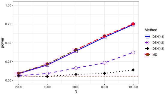
Figure 1.
Power comparison of the MD test and DZH test based on different bandwidths under model M2 with and . Error term is generated from standard normal distribution.
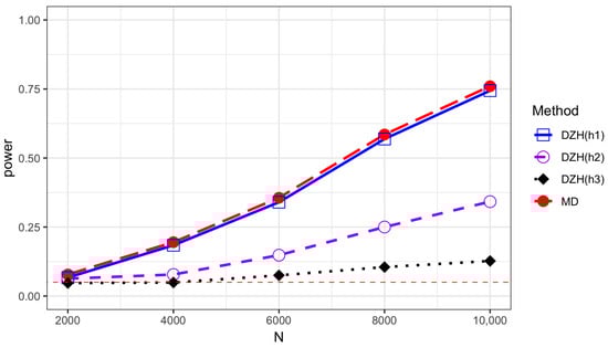
Figure 2.
Power comparison of the MD test and DZH test based on different bandwidths under model M2 with and . Error term is generated from standardized exponential distribution.
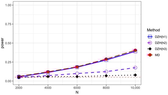
Figure 3.
Power comparison of the MD test and DZH test based on different bandwidths under model M2 with and . Error term is generated from Student’s t distribution with 5 degrees of freedom.
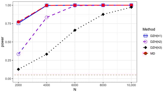
Figure 4.
Power comparison of the MD test and DZH test based on different bandwidths under model M2 with and . Error term is generated from standard normal distribution. and are generated from Student’s t distribution with 5 degrees of freedom.
5. Proofs
Some Lemmas
In this section, we restate three Lemmas in Zhao et al. [18], omitting detailed proofs for brevity. Lemma 2 is restated under assumption . We assume without loss of generality. Denote
We introduce the following matrix notations:
Under , ,
Under , , then , where . Following Zhao et al. [18], we decompose in the following way:
Lemma 1.
Given Assumptions 1–5, under the null hypothesis, can be consistently estimated by , as , , .
Lemma 2.
Given Assumptions 1–5,
1. uniformly for under , as , , .
2. , uniformly for under and , as , , .
3. , uniformly for under and , as , , .
Lemma 3.
Denote . Under Assumptions 1–6, for any and n large enough, where , we have
When
we have
Proof of Theorem 2.
We first construct a alternative based on .
Using the method in Guerre and Lavergne [13] to construct the alternatives , define
for .
Then, , without loss of generality, we assume that is an integer. Let
where are orthogonal with disjoint supports , and is bounded and nonnegative. Let be any sequence with ,
Under Assumption 3, we have that there exists a constant C such that and . Since
for any . The main idea is that if cannot be consistent against alternatives as , then we can conclude that it also not consistent uniformly against as .
Based on Lemma 1–3, the test statistic
Without loss of generality, we assume that has support in the following proofs:
(i): For .
(ii): For .
Through tedious calculation, we can also get and as for above two cases. Therefore, for any , there exists such that as . Therefore, we cannot get . We obtain the same conclusion for . Thus, the theorem is proved. □
Author Contributions
Conceptualization, Y.Z.; methodology, Y.Z.; formal analysis, P.L. and Y.Z.; investigation, Y.Z. and L.X.; writing—original draft preparation, P.L. and Y.Z.; writing—review and editing, P.L., Y.Z. and L.X.; visualization, P.L., Y.Z. and T.W.; supervision, Y.Z. All authors have read and agreed to the published version of the manuscript.
Funding
This study was supported by the National Natural Science Foundation of China (12201351) and the Natural Science Foundation of Shandong Province (ZR2022QA013), as well as the Natural Science Foundation of the Jiangsu Higher Education Institutions of China (24KJB110024) the Qinglan Project of Jiangsu Province of China [2022], and the Huai’an City Science and Technology Project (HAB202357).
Institutional Review Board Statement
Not applicable.
Data Availability Statement
No new data were created or analyzed in this study. Data sharing is not applicable to this article.
Conflicts of Interest
The authors declare no conflicts of interest. The funders had no role in the design of the study; in the collection, analyses, or interpretation of data; in the writing of the manuscript; or in the decision to publish the results.
References
- Zaremba, W.; Gretton, A.; Blaschko, M. B-test: A Non-parametric, Low Variance Kernel Two-sample Test. Adv. Neural Inf. Process. Syst. 2013, 26, 755–763. [Google Scholar]
- Chen, X.Y.; Xie, M.G. A split-and-conquer approach for analysis of extraordinarily large data. Stat. Sin. 2014, 24, 1655–1684. [Google Scholar]
- Battey, H.; Fan, J.; Liu, H.; Lu, J.; Zhu, Z. Distributed Estimation and Inference with Statistical Guarantees. arXiv 2015, arXiv:1509.05457. [Google Scholar]
- Fan, J.; Han, F.; Liu, H. Challenges of Big Data analysis. Natl. Sci. Rev. 2014, 1, 293–314. [Google Scholar] [CrossRef] [PubMed]
- Hardle, W.; Mammen, E. Comparing nonparametric versus parametric regression fits. Ann. Statist. 1993, 21, 1926–1947. [Google Scholar] [CrossRef]
- Neumeyer, N.; Van Keilegom, I. Estimating the error distribution in nonparametric multiple regression with applications to model testing. J. Multivar. Anal. 2010, 101, 1067–1078. [Google Scholar] [CrossRef]
- González-Manteiga, W.; Crujeiras, R.M. An updated review of Goodness-of-Fit tests for regression models. Test 2013, 22, 361–411. [Google Scholar] [CrossRef] [PubMed]
- Delgado, M. Testing the equality of nonparametric regression curves. Stat. Probab. Lett. 1993, 17, 199–204. [Google Scholar] [CrossRef]
- Bierens, H.J. A consistent conditional moment test of functional form. Econometrica 1990, 58, 1443–1458. [Google Scholar] [CrossRef]
- Hart, J.D. Nonparametric Smoothing and Lack-of-Fit Tests, 1st ed.; Springer: New York, NY, USA, 1997. [Google Scholar]
- Ingster, Y.I. Minimax nonparametric detection of signals in white Gaussian noise. Probl. Inf. Transm. 1982, 18, 130–140. [Google Scholar]
- Ingster, Y.I. Asymptotically minimax hypothesis testing for nonparametric alternatives I, II, III. Math. Methods Stat. 1993, 2, 85–114. [Google Scholar]
- Guerre, E.; Lavergne, P. Optimal minimax rates for nonparametric specification testing in regression models. Econom. Theory 2002, 18, 1139–1171. [Google Scholar] [CrossRef]
- Cai, L.; Guo, X.; Zhong, W. Test and Measure for Partial Mean Dependence Based on Machine Learning Methods. J. Am. Stat. Assoc. 2024, 1–13. [Google Scholar] [CrossRef]
- Tan, F.; Zhu, L. Adaptive-to-model checking for regressions with diverging number of predictors. Ann. Stat. 2019, 47, 1960–1994. [Google Scholar] [CrossRef]
- Han, Y.; Ma, P.; Ren, H.; Wang, Z. Model checking in large-scale data set via structure-adaptive-sampling. Stat. Sin. 2023, 33, 303–329. [Google Scholar]
- Zheng, J.X. A consistent test of functional form via nonparametric estimation techniques. J. Econom. 1996, 75, 263–289. [Google Scholar] [CrossRef]
- Zhao, Y.; Zou, C.; Wang, Z. A scalable nonparametric specification testing for massive data. J. Stat. Plan. Inference 2019, 200, 161–175. [Google Scholar] [CrossRef]
- Zhao, Y.; Zou, C.; Wang, Z. An adaptive lack of fit test for big data. Stat. Theory Relat. Fields 2017, 1, 59–68. [Google Scholar] [CrossRef]
- Ibragimov, I.A.; Khasminski, R.Z. Statistical Estimation: Asymptotic Theory, 1st ed.; Springer: Berlin/Heidelberg, Germany, 1981. [Google Scholar]
- Horowitz, J.; Spokoiny, V. An adaptive, rate-optimal test of parametric mean-regression model against a nonparametric alternative. Econometrica 2001, 69, 599–631. [Google Scholar] [CrossRef]
- Guerre, E.; Lavergne, P. Data-driven rate-optimal specification testing in regression models. Ann. Stat. 2005, 33, 840–870. [Google Scholar] [CrossRef]
Disclaimer/Publisher’s Note: The statements, opinions and data contained in all publications are solely those of the individual author(s) and contributor(s) and not of MDPI and/or the editor(s). MDPI and/or the editor(s) disclaim responsibility for any injury to people or property resulting from any ideas, methods, instructions or products referred to in the content. |
© 2025 by the authors. Licensee MDPI, Basel, Switzerland. This article is an open access article distributed under the terms and conditions of the Creative Commons Attribution (CC BY) license (https://creativecommons.org/licenses/by/4.0/).