Fractional Evolution Equation with Nonlocal Multi-Point Condition: Application to Fractional Ginzburg–Landau Equation

Abstract

This paper is devoted to studying the existence and uniqueness of mild solutions for semilinear fractional evolution equations with the Hilfer–Katugampola fractional derivative and under the nonlocal multi-point condition. The analysis is based on analytic semigroup theory, the Krasnoselskii fixed-point theorem, and the Banach fixed-point theorem. An application to a time-fractional real Ginzburg–Landau equation is also given to illustrate the applicability of our results. Furthermore, we determine some conditions to make the control (Bifurcation) parameter in the Ginzburg–Landau equation sufficiently small.

1. Introduction

In mathematics, the abstract formulation of dynamic partial differential equations can be thought of as evolution equations over an infinite-dimensional state space. Evolution equations can be found in many sectors of applied science and engineering. Nonlinear evolution equations include the Schrödinger equation in quantum mechanics, degenerate Navier–Stokes equations in fluid dynamics, and Reaction–Diffusion equations in heat transport and life sciences [1,2,3].

The fractional evolution equation provides a powerful mathematical framework for investigating complicated systems with fractional-order derivatives. One variant is known as the Hilfer–Katugampola fractional derivative. The Hilfer–Katugampola fractional derivative is a broader version of fractional calculus that includes both the Hilfer and Katugampola derivatives. It provides a more flexible framework by merging aspects of several fractional derivatives, such as Riemann–Liouville derivatives, Caputo-type derivatives, and the Hadamard fractional derivative [4,5,6,7].

Research on fractional evolution equations has been presented in many articles [8,9,10,11,12]. Zhou and Jiao [8] discussed a class of fractional neutral evolution equations with nonlocal conditions and obtained various criteria on the existence and uniqueness of mild solutions. In 2021, the authors of [9] proved the existence and uniqueness of a mild solution to a system of $\psi$-Hilfer neutral fractional evolution equations with infinite delay. The local and global existence and uniqueness of mild solutions to initial value problems for fractional semilinear evolution equations with compact and noncompact semigroups in Banach spaces were examined by the authors of [10]. In 2022, the authors of [11] obtained the mild solution using the $\rho$-Laplace transform and strongly continuous cosine and sine families of uniformly bounded linear operators.

In our work, we present the fractional evolution equation given as follows:

$${}^{\rho }D^{\alpha ,\beta }x\left(t\right)-Ax\left(t\right)=g(t,x\left(t\right)),t\in [0,b],$$

(1a)

$${}^{\rho }I^{1-\gamma }x{\left(t\right)}_{{|}_{t=0}}=\sum _{i=1}^m{c}_{i}x\left({\tau }_i\right),m\in \mathbb{N}$$

(1b)

where

• $x(·)$: The state function in Banach space $\mathbb{X}$ equipped with the norm ${\parallel ·\parallel }_{\mathbb{X}}$;
• ${}^{\rho }D^{\alpha ,\beta }$: A Hilfer–Katugampola fractional derivative of order $\alpha \in (0,1)$ and types $\beta \in [0,1]$ and $\rho >0$;
• ${}^{\rho }I^{1-\gamma }$: A Katugampola fractional integral of order $1-\gamma$ with $\gamma =\alpha +\beta (1-\alpha )$;
• A: An infinitesimal generator of $C_0$ semigroup in a Banach space $\mathbb{X}$;
• $g:[0,b]\times \mathbb{X}\to \mathbb{X}$: The continuous function in a Banach space $\mathbb{X}$;
• $c_i,i=1,2,\dots m;m\in \mathbb{N}$ are real constants;
• ${\tau }_i,i=1,2,\dots m;m\in \mathbb{N}$ are positive real constants such that $0\le {\tau }_1<{\tau }_2<\cdots <{\tau }_m\le b$.

In this context, it should be noted that Condition (1b) was introduced by Byszewski [13] and used later by several contributors; for example, see [14,15,16,17,18,19,20] and the contributions given therein. This nonlocal condition allows for a broader and more flexible description of the system, which can be especially useful in modeling complex physical phenomena. For example, in diffusion processes, where the system’s behavior depends not just on its initial state but also on how it has evolved over time, this kind of nonlocal condition can provide a more accurate representation. In the case of gas diffusion in a transparent tube, the nonlocal condition might account for the gas concentration at various previous times rather than just the initial state [21].

One of the most significant nonlinear equations in physics is the Ginzburg–Landau equation, which describes how minor shocks transform a system without linearity from a stable to an unstable state. One particular instance of the generic Ginzburg–Landau equation is the real Ginzburg–Landau equation. It was employed to simulate a wide range of physical processes, including nonlinear waves, liquid crystals, second-order phase transitions, Bose–Einstein condensation, superconductivity, superfluidity, and strings in field theory. Also, the evolution of disturbances in systems going through a transition from a stable to an unstable state, especially close to a finite-wavelength bifurcation, is described by this nonlinear partial differential equation. The actual Ginzburg–Landau equation in the setting of non-oscillatory bifurcations is written as follows [22]:

$${\displaystyle \frac{\partial \mathfrak{A}}{\partial t}}={\nabla }^2\mathfrak{A}+\sigma \mathfrak{A}-\mathfrak{A}{\left|\mathfrak{A}\right|}^2,$$

in which $\sigma$, $\mathfrak{A}$, and ${\nabla }^2$ indicate the control parameter, the disturbance’s amplitude, and the Laplacian operator. Newell and Whitehead [23] and Segel [24] were the first to obtain these results with a control parameter $\sigma$.

Using conformable fractional derivatives, Raza [25] built the conformable time-fractional Ginzburg–Landau equation and discovered new explicit, periodic, and accurate solutions with Kerr law nonlinearity. Furthermore, [26] used the generalized projective Riccati equation approach to examine the fractional effects of a complex Ginzburg–Landau model with quadratic-cubic, anti-cubic, and generalized anti-cubic laws of nonlinearity. To successfully derive several exact solutions for the time-fractional Ginzburg–Landau equation with Kerr law nonlinearity, Murad et al. [27] used a novel variation of the Sardar sub-equation approach. As an application, the solvability of the time-fractional Ginzburg–Landau equation with the Hilfer–Katugampola fractional derivative can be examined using our results to illustrate their applicability.

A unified framework for examining the well-posedness of complex systems of different kinds that describe the time evolution of concrete systems (like time-fractional diffusion equations) is provided by fractional evolution equations. Two strong arguments support the need to look into this class of equations: differential models that use the fractional derivative to describe memory and hereditary properties are a great tool, and they have recently been shown to be useful tools for modeling a variety of physical phenomena. Since the fractional derivative provides a more realistic representation of some systems, fractional-order models of actual systems are always more suitable than traditional integer-order models. Additionally, many of the phenomena studied in hybrid systems, such as dry friction, controlled heat transfer processes, obstruction difficulties, and others, may be explained by a variety of differential equations, both linear and nonlinear [28,29,30].

2. Preliminaries

In this section, we briefly introduce some basic definitions, theorems, and results that are important to the study of the $\rho$-Laplace transform. We include some definitions and results on the Hilfer–Katugampola fractional derivative. Most of the material can be found in [31]. Other useful references in this regard are [32,33].

2.1. Fractional Calculus

Suppose the space ${\mathbb{X}}_c^p(a,b),(c\in \mathbb{R},1\le p<\infty )$ of Lebesgue measurable of complex-valued function f on the interval $[a,b]$ equipped with the norm

$${\parallel f\parallel }_{{\mathbb{X}}_c^p}={\left({\int }_a^b{\left|x^{c}f\left(x\right)\right|}^p{\displaystyle \frac{dx}{x}}\right)}^{{\displaystyle \frac{1}{p}}}.$$

Moreover, by $\mathcal{C}\left(\right[a,b],\mathbb{R})$ we denote the Banach space of all continuous functions from $[a,b]$ into $\mathbb{R}$ and we define the weighted Banach space

$$\begin{array}{c}\hfill {\mathcal{C}}_{\gamma ,\rho }([a,b],\mathbb{R})=\left\{f:[a,b]\to \mathbb{R}:{\left({\displaystyle \frac{x^{\rho }-a^{\rho }}{\rho }}\right)}^{\gamma }f\left(x\right)\in \mathcal{C}([a,b],\mathbb{R})\right\},\end{array}$$

for all $x\in [a,b]$ and $0\le \gamma <1$, equipped with the norm

$${\parallel f\parallel }_{{\mathcal{C}}_{\gamma ,\rho }}=\underset{x\in [a,b]}{sup}\left\{{\left({\displaystyle \frac{x^{\rho }-a^{\rho }}{\rho }}\right)}^{\gamma }\left|f\left(x\right)\right|\right\}.$$

Definition 1

([32] Katugampola fractional integral). Let $f\in {\mathbb{X}}_c^p(a,b)$. Then, the left Katugampola fractional integral of order $\alpha >0$ and type $\rho >0$ is defined by

$${(}^{\rho }{I}_{a^{+}}^{\alpha }f)\left(x\right)={\displaystyle \frac{1}{\mathsf{\Gamma }\left(\alpha \right)}}{\int }_a^x{\left({\displaystyle \frac{x^{\rho }-t^{\rho }}{\rho }}\right)}^{\alpha -1}f\left(t\right){\displaystyle \frac{dt}{t^{1-\rho }}},x>a.$$

Definition 2

([32] Katugampola fractional derivative). Let $f\in {\mathbb{X}}_c^p(a,b)$. Then, the left Katugampola fractional derivative of order $\alpha \in {\mathbb{R}}_{+}$ and type $\rho >0$ is defined by

$$\begin{array}{cc}\hfill \left({}^{\rho }D_{a^{+}}^{\alpha }f\right)\left(x\right)& ={\delta }_{\rho }^n\left({}^{\rho }I_{a^{+}}^{n-\alpha }f\right)\left(x\right)\hfill \\ \hfill & ={\displaystyle \frac{1}{\mathsf{\Gamma }(n-\alpha )}}{\left(x^{1-\rho }{\displaystyle \frac{d}{dx}}\right)}^n{\int }_a^x{\left({\displaystyle \frac{x^{\rho }-t^{\rho }}{\rho }}\right)}^{n-\alpha -1}f\left(t\right){\displaystyle \frac{dt}{t^{1-\rho }}},x>a,\hfill \end{array}$$

where $n-1<\alpha <n$, $n\in \mathbb{N}$ and ${\delta }_{\rho }=x^{1-\rho }{\displaystyle \frac{d}{dx}}$.

Lemma 1

([32]). Let $f\in {\mathbb{X}}_c^p(a,b)$ and $\alpha ,\beta ,\rho >0$. Then, the Katugampola fractional integral and derivative satisfy the properties

$$\begin{array}{cc}\hfill \left({}^{\rho }I_{a^{+}}^{\alpha }{}^{\rho }I_{a^{+}}^{\beta }f\right)\left(x\right)& =\left({}^{\rho }I_{a^{+}}^{\alpha +\beta }f\right)\left(x\right)\hfill \\ \hfill \left({}^{\rho }D_{a^{+}}^{\alpha }{}^{\rho }I_{a^{+}}^{\alpha }f\right)\left(x\right)& =f\left(x\right).\hfill \end{array}$$

Moreover,

$$\begin{array}{cc}\hfill {}^{\rho }I_{a^{+}}^{\alpha }{\left({\displaystyle \frac{x^{\rho }-a^{\rho }}{\rho }}\right)}^{\beta -1}& ={\displaystyle \frac{\mathsf{\Gamma }\left(\beta \right)}{\mathsf{\Gamma }(\beta +\alpha )}}{\left({\displaystyle \frac{x^{\rho }-a^{\rho }}{\rho }}\right)}^{\beta +\alpha -1}\hfill \\ \hfill {}^{\rho }D_{a^{+}}^{\alpha }{\left({\displaystyle \frac{x^{\rho }-a^{\rho }}{\rho }}\right)}^{\beta -1}& ={\displaystyle \frac{\mathsf{\Gamma }\left(\beta \right)}{\mathsf{\Gamma }(\beta -\alpha )}}{\left({\displaystyle \frac{x^{\rho }-a^{\rho }}{\rho }}\right)}^{\beta -\alpha -1}\hfill \\ \hfill {}^{\rho }D_{a^{+}}^{\alpha }{\left({\displaystyle \frac{x^{\rho }-a^{\rho }}{\rho }}\right)}^{\alpha -1}& =0.\hfill \end{array}$$

Lemma 2.

Let $\alpha >0$, and $0\le \gamma <1$. Then, ${}^{\rho }I_{a^{+}}^{\alpha }$ is bounded from ${\mathcal{C}}_{\gamma ,\rho }\left([a,b]\right)$ into ${\mathcal{C}}_{\gamma ,\rho }\left([a,b]\right)$.

Definition 3

([34] Hilfer–Katugampola fractional derivative). The Hilfer–Katugampola fractional derivative of order $n-1<\alpha <n,n\in \mathbb{N}$ and type $0\le \beta \le 1$ with a parameter $\rho >0$ for a function $f\in {\mathcal{C}}_{1-\nu ,\rho }[a,b]$ with $0<\nu <1$, is defined by

$$\begin{array}{c}\hfill \left({}^{\rho }D_{a^{+}}^{\alpha ,\beta }f\right)\left(x\right)=\left({}^{\rho }I_{a^{+}}^{\beta (n-\alpha )}{\delta }_{\rho }^n{}^{\rho }I_{a^{+}}^{(1-\beta )(n-\alpha )}f\right)\left(x\right).\end{array}$$

Remark 1

(Property 3.2 in [34]). If $0<\alpha <1$ and $f\in {\mathcal{C}}_{1-\gamma ,\rho }[a,b]$, the Hilfer–Katugampola fractional derivative takes the form

$$\left({}^{\rho }D_{a^{+}}^{\alpha ,\beta }f\right)\left(x\right)=\left({}^{\rho }I_{a^{+}}^{\beta (1-\alpha )}{}^{\rho }D_{a^{+}}^{\gamma }f\right)\left(x\right),\gamma =\alpha +\beta (1-\alpha ).$$

It is obvious that $0<\gamma \le \alpha$ and $\gamma \le \beta$.

Lemma 3

([32]). Let $0<\alpha <1,0\le \beta \le 1$ and $\gamma =\alpha +\beta (1-\alpha )$. If $f\in {\mathcal{C}}_{1-\gamma ,\rho }\left([0,b]\right)$. Then,

$$\begin{array}{cc}\hfill \left({}^{\rho }I_{a^{+}}^{\gamma }{}^{\rho }D_{a^{+}}^{\gamma }f\right)\left(x\right)& =\left({}^{\rho }I_{a^{+}}^{\alpha }{}^{\rho }D_{a^{+}}^{\alpha ,\beta }f\right)\left(x\right),\hfill \\ \hfill \left({}^{\rho }D_{a^{+}}^{\gamma }{}^{\rho }I_{a^{+}}^{\alpha }f\right)\left(x\right)& =\left({}^{\rho }D_{a^{+}}^{\beta (1-\alpha )}f\right)\left(x\right).\hfill \end{array}$$

Theorem 1

(Lebesgue dominated convergence theorem [35]). Let E be a measurable set and let $\left\{f_n\right\}$ be a sequence of measurable functions such that ${lim}_{n\to \infty }{f}_n=f\left(x\right)$ pointwise almost everywhere in E, and for every $n\in \mathbb{N}$, $|f_n\left(x\right)|\le g\left(x\right)$ pointwise almost everywhere in E, where g is integrable on E. Then

$$\underset{n\to \infty }{lim}{\int }_E{f}_n\left(x\right)dx={\int }_{E}f\left(x\right)dx.$$

Lemma 4

(Arzela–Ascoli’s theorem). If a family $F=\left\{f\right(t\left)\right\}$ in $\mathcal{C}(E,\mathbb{X})$ is uniformly bounded and equicontinuous on E, and for any $t\in E$, $\left\{f\left(t^{*}\right)\right\}$ is relatively compact, then F has a uniformly convergent subsequence ${\left\{f_n\left(t\right)\right\}}_{n=1}^{\infty }$.

Remark 2.

Arzela–Ascoli’s theorem is the key to the following result: A subset F in $\mathcal{C}(E,\mathbb{R})$ is relatively compact if and only if it is uniformly bounded and equicontinuous on E.

Lemma 5

(Neumann’s Lemma [36]). Let $\mathbb{X}$ be an arbitrary Banach space, and let $T\in B\left(\mathbb{X}\right)$ be a bounded linear operator with operator norm $\parallel T\parallel <1$. Then, the following statements hold.

• The infinite series ${\sum }_{k=0}^{\infty }{T}^k$ is called the Neumann series, and it is also an element in $B\left(\mathbb{X}\right)$.
• The operator $(I-T)$ has a bounded inverse operator ${(I-T)}^{-1}={\sum }_{k=0}^{\infty }{T}^k$ on $\mathbb{X}$.
• ${\parallel (I-T)}^{-1}\parallel \le {\displaystyle \frac{1}{1-\parallel T\parallel }}$.

Theorem 2

(Fredholm alternative theorem). Let $\mathbb{X}$ be a Banach space, $T:\mathbb{X}\to \mathbb{X}$ be a compact operator, and $\lambda \in \mathbb{C}$ be non-zero. Then, exactly one of the following statements holds:

• (Eigenvalue) There is a non-trivial solution $x\in \mathbb{X}$ to the equation $Tx=\lambda x$.
• (Bounded resolvent) The operator $T-\lambda$ has a bounded inverse ${(T-\lambda )}^{-1}$ on $\mathbb{X}$.

Theorem 3

(Gronwall inequality [37]). Let $u,v$ be two integrable functions and g be a continuous function, with domain $[a,b]$. Assume that:

• u and v are nonnegative;
• g is nonnegative and nondecreasing.

If

$$u\left(t\right)\le v\left(t\right)+g\left(t\right){\rho }^{1-\alpha }{\int }_a^t{s}^{\rho -1}{\left(t^{\rho }-s^{\rho }\right)}^{\alpha -1}u\left(s\right)ds,t\in [a,b],$$

Then,

$$u\left(t\right)\le v\left(t\right)+{\int }_a^t\sum _{k=1}^{\infty }{\displaystyle \frac{{\rho }^{1-k\alpha }{\left[g\left(t\right)\mathsf{\Gamma }\left(\alpha \right)\right]}^k}{\mathsf{\Gamma }\left(\alpha k\right)}}{s}^{\rho -1}{[t^{\rho }-s^{\rho }]}^{\alpha k-1}v\left(s\right)ds,t\in [a,b].$$

In addition, if v is nondecreasing. Then,

$$u\left(t\right)\le v\left(t\right)E_{\alpha }\left[g\left(t\right)\mathsf{\Gamma }\left(\alpha \right){\left({\displaystyle \frac{t^{\rho }-a^{\rho }}{\rho }}\right)}^{\alpha }\right],\forall t\in [a,b],$$

where

$$E_{\alpha }\left(x\right)=\sum _{r=0}^{\infty }{\displaystyle \frac{x^r}{\mathsf{\Gamma }(\alpha r+1)}},\alpha >0,x\in \mathbb{R}.$$

denotes the Mittag-Leffler function.

2.2. $\rho$-Laplace Transform

This subsection is devoted to recalling the definition of the $\rho$-Laplace transform and some of its properties, which are shown in [31,38].

Definition 4.

A function $f:[0,\infty )\to \mathbb{R}$ is said to be of ρ-exponential order $exp\left(c{\displaystyle \frac{t^{\rho }}{\rho }}\right)$ if there exist nonnegative constants $M,c,T$ such that

$$\left|f\left(t\right)\right|\le Mexp\left(c{\displaystyle \frac{t^{\rho }}{\rho }}\right),t\ge T.$$

Definition 5

([38]). Let $f:[0,\infty )\to \mathbb{R}$ be a piecewise continuous function and of ρ-exponential order $exp\left(c{\displaystyle \frac{t^{\rho }}{\rho }}\right)$. Then, the ρ-Laplace transform is defined by

$$\mathcal{L}\left\{f\left(t\right)\right\}\left(\lambda \right)=F_{\rho }\left(\lambda \right)={\int }_{t_0}^{\infty }{e}^{-\lambda {\displaystyle \frac{{(t-t_0)}^{\rho }}{\rho }}}f\left(t\right){(t-t_0)}^{\rho -1}dt,$$

for all values of $\lambda >c$.

Lemma 6.

If the ρ-Laplace transform of $f:[0,\infty )\to \mathbb{R}$ exists for $\lambda >c_1$ and the ρ-Laplace transform of $g:[0,\infty )\to \mathbb{R}$ exists for $\lambda >c_2$. Then, for any constants a and b, the ρ-Laplace transform of $af+bg$ exists and

$$\mathcal{L}\{af\left(t\right)+bg\left(t\right)\}\left(\lambda \right)=a\mathcal{L}\left\{f\left(t\right)\right\}\left(\lambda \right)+b\mathcal{L}\left\{g\left(t\right)\right\}\left(\lambda \right),\lambda >max\{c_1,c_2\}.$$

Definition 6.

Let f and g be two piecewise continuous functions on the interval $[0,T]$ and of ρ-exponential order. Then, the ρ-convolution of f and g is defined by

$$\left(f{\ast }_{\rho }g\right)\left(t\right)={\int }_0^{t}f\left({(t^{\rho }-{\tau }^{\rho })}^{{\displaystyle \frac{1}{\rho }}}\right)g\left(\tau \right){\displaystyle \frac{d\tau }{{\tau }^{1-\rho }}}.$$

Lemma 7.

Let f and g be two piecewise continuous functions on the interval $[0,T]$ and of ρ-exponential order. Then,

$$\mathcal{L}\left\{f{\ast }_{\rho }g\right\}=\mathcal{L}\left\{f\right\}\mathcal{L}\left\{g\right\}.$$

Lemma 8.

Let $\alpha >0$ and f be a piecewise continuous function on the interval $[0,T]$ and of ρ-exponential order $exp\left(c{\displaystyle \frac{t^{\rho }}{\rho }}\right)$. Then,

$$\mathcal{L}\left\{{(}^{\rho }{I}_{0^{+}}^{\alpha }f)\left(t\right)\right\}\left(\lambda \right)={\lambda }^{-\alpha }\mathcal{L}\left\{f\left(t\right)\right\}\left(\lambda \right),\lambda >c.$$

Lemma 9.

Let $\alpha >0$ and $f\in A{\mathcal{C}}_{\gamma }^n[0,b]$ for any $b>0$ and $I_{0^{+}}^{n-k-1}f,k=0,1,\dots ,n-1$ be of ρ-exponential order $exp\left(c{\displaystyle \frac{t^{\rho }}{\rho }}\right)$. Then

$$\mathcal{L}\left\{{(}^{\rho }{D}_{0^{+}}^{\alpha }f)\left(t\right)\right\}={\lambda }^{\alpha }\mathcal{L}\left\{f\left(t\right)\right\}-\sum _{k=0}^{n-1}{\lambda }^{n-k-1}\left(I_{0^{+}}^{n-k-1}f\right)\left(0\right),\lambda >c.$$

Proposition 1

($\rho$-Laplace transform to Hilfer–Katugampola derivative). Let order α and type β satisfy $0<\alpha <1$ and $0\le \beta \le 1$. The ρ-Laplace transform of Hilfer–Katugampola fractional derivative (left-sided), with respect to t, with $\rho >0$ of a function $f\in {\mathcal{C}}_{1-\gamma ,\rho }([0,T],\mathbb{R})$, is defined by

$$\mathcal{L}\left\{{}^{\rho }D_{0^{+}}^{\alpha ,\beta }\right\}f\left(t\right)={\lambda }^{\alpha }{F}_{\rho }\left(\lambda \right)-{\lambda }^{\beta (\alpha -1)}{}^{\rho }I_{0^{+}}^{1-\gamma }f\left(0\right).$$

Proof. 

Using Remark 1 and Lemma 8, we can write

$$\begin{array}{cc}\hfill \mathcal{L}{\{}^{\rho }{D}_{0^{+}}^{\alpha ,\beta }f\left(t\right)\}\left(\lambda \right)& =\mathcal{L}{\{}^{\rho }{I}_{0^{+}}^{\beta (1-\alpha )}g\left(t\right)\}\left(\lambda \right)\hfill \\ \hfill & ={\lambda }^{-\beta (1-\alpha )}\mathcal{L}\left\{g\left(t\right)\right\}\hfill \end{array}$$

where $g\left(t\right){=}^{\rho }{D}_{0^{+}}^{\gamma }f\left(t\right)$ and $\gamma =\alpha +\beta (1-\alpha )$. In view of Lemma 9, we obtain

$$\mathcal{L}\left\{g\left(t\right)\right\}\left(\lambda \right)=\mathcal{L}{\{}^{\rho }{D}_{0^{+}}^{\gamma }f\left(t\right))\}\left(\lambda \right)={\lambda }^{\gamma }\mathcal{L}\left\{f\left(t\right)\right\}\left(\lambda \right){-}^{\rho }{I}_{0^{+}}^{1-\gamma }f\left(0\right).$$

This gives the desired result. □

2.3. $C_0$ Semigroup

In this subsection, some needed definitions and results about $C_0$ semigroup are provided to be a helper for proving our results and taken from [39].

Definition 7.

Let $\mathbb{X}$ be a Banach space. A one-parameter family ${\left\{Q\left(t\right)\right\}}_{t\ge 0}$ from $\mathbb{X}$ into $\mathbb{X}$ is a semigroup of bounded linear operators on $\mathbb{X}$ if

• $Q(t+s)=Q\left(t\right)Q\left(s\right)$ where $t,s\ge 0$ (the semigroup property);
• $Q\left(0\right)=I$, where I is the identity operator in $\mathbb{X}$.

Lemma 10.

Let A be the generator of a strongly continuous semigroup $Q\left(t\right)$ for all $t\ge 0$ on a Banach space $\mathbb{X}$. Then, there exist constants $M\ge 1$ and $\omega >0$ with

$$\begin{array}{c}\hfill \parallel Q\left(t\right)x\parallel \le M{e}^{\omega t}\parallel x\parallel ,t\ge 0.\end{array}$$

Definition 8.

Let $A:D\left(A\right)\subset \mathbb{X}\to \mathbb{X}$ be a linear operator on a $\mathbb{K}$-Banach space $\mathbb{X}$ with $\mathbb{K}$ = $\mathbb{R}$ or $\mathbb{C}$. The resolvent set $\rho \left(A\right)$ of the operator A is the set of all points $\lambda \in \mathbb{K}$ such that $\lambda I-A$ is a bijection from $D\left(A\right)$ into $\mathbb{X}$ and its resolvent operator exists and

$$R(\lambda ,A)={(\lambda I-A)}^{-1}.$$

Lemma 11.

Let A be the generator of a strongly continuous semigroup $Q\left(t\right)$. Then,

$$R(\lambda ,A)={\int }_0^{\infty }{e}^{-\lambda t}Q\left(t\right)dt,\lambda \in \rho \left(A\right).$$

Definition 9.

Let the function

$$\begin{array}{c}\hfill {\psi }_{\alpha }\left(\theta \right)={\displaystyle \frac{\alpha }{{\theta }^{\alpha +1}}}{M}_{\alpha }\left({\theta }^{-\alpha }\right),\theta \in (0,\infty ),0<\alpha <1\end{array}$$

where $M_{\alpha }$ is the Wright function defined by

$$\begin{array}{c}\hfill M_{\alpha }\left(\theta \right)={\displaystyle \frac{1}{\pi }}\sum _{n=0}^{\infty }{(-1)}^{n-1}{\theta }^{-\alpha n-1}{\displaystyle \frac{\mathsf{\Gamma }(n\alpha +1)}{n!}}sin\left(n\pi \alpha \right),0<\alpha <1.\end{array}$$

It is known that

$$\begin{array}{ccc}\hfill {\int }_0^{\infty }{\theta }^{\delta }{M}_{\alpha }\left(\theta \right)d\theta & ={\displaystyle \frac{\mathsf{\Gamma }(\delta +1)}{\mathsf{\Gamma }(\delta \alpha +1)}},\hfill & \hfill \delta >-1,0<\alpha <1,\\ \hfill {\int }_0^{\infty }{e}^{-\lambda \theta }{\psi }_{\alpha }\left(\theta \right)d\theta & =e^{-{\lambda }^{\alpha }},\hfill & \hfill \lambda >0,0<\alpha <1.\end{array}$$

3. Construct of Mild Solution and Some Properties

To study problem (1), we need to determine the existence of a mild solution of the following linear problem:

$$\begin{array}{cc}\hfill {}^{\rho }D^{\alpha ,\beta }x\left(t\right)& =Ax\left(t\right)+g\left(t\right),t\in [0,b],\hfill \end{array}$$

(2a)

$$\begin{array}{cc}\hfill {}^{\rho }I^{1-\gamma }x\left(0\right)& =x_0.\hfill \end{array}$$

(2b)

Theorem 4.

The mild solution of the fractional evolution Equation (2) has the form

$$\begin{array}{c}\hfill \begin{array}{cc}\hfill x\left(t\right)& =S_{\beta ,\alpha }\left(t\right)x_0+{\int }_0^t{K}_{\alpha }\left({(t^{\rho }-s^{\rho })}^{{\displaystyle \frac{1}{\rho }}}\right)g\left(s\right){\displaystyle \frac{ds}{s^{1-\rho }}}\hfill \end{array}\end{array}$$

(3)

where

$$\begin{array}{cc}\hfill K_{\alpha }\left(t\right)& =\alpha {\left({\displaystyle \frac{t^{\rho }}{\rho }}\right)}^{\alpha -1}{\int }_0^{\infty }\theta M_{\alpha }\left(\theta \right)Q\left({\left({\displaystyle \frac{t^{\rho }}{\rho }}\right)}^{\alpha }\theta \right)d\theta ,\hfill \\ \hfill S_{\beta ,\alpha }\left(t\right)& ={}^{\rho }I^{\beta (1-\alpha )}{K}_{\alpha }\left(t\right).\hfill \end{array}$$

Proof. 

Applying the $\rho$-Laplace transform with $\lambda >0$ in Cauchy problem (2) yields

$$\begin{array}{c}\hfill \begin{array}{cc}\hfill ({\lambda }^{\alpha }-A)X_{\rho }\left(\lambda \right)& ={\lambda }^{\beta (\alpha -1)}{x}_0+G\left(\lambda \right).\hfill \end{array}\end{array}$$

(4)

where

$$\begin{array}{c}\hfill X_{\rho }\left(\lambda \right)={\int }_0^{\infty }{e}^{{\displaystyle \frac{-\lambda t^{\rho }}{\rho }}}x\left(t\right){\displaystyle \frac{dt}{t^{1-\rho }}},G_{\rho }\left(\lambda \right)={\int }_0^{\infty }{e}^{{\displaystyle \frac{-\lambda t^{\rho }}{\rho }}}g\left(t\right){\displaystyle \frac{dt}{t^{1-\rho }}}.\end{array}$$

By using the concept of the resolvent operator with ${\lambda }^{\alpha }\in \rho \left(A\right)$, the Equation (4) is equivalent to

$$\begin{array}{c}\hfill \begin{array}{cc}\hfill X_{\rho }\left(\lambda \right)& ={\lambda }^{-\beta (1-\alpha )}R({\lambda }^{\alpha },A)x_0+R({\lambda }^{\alpha },A)G_{\rho }\left(\lambda \right),\hfill \\ & ={\lambda }^{-\beta (1-\alpha )}{\int }_0^{\infty }{e}^{-{\lambda }^{\alpha }s}Q\left(s\right)x_{0}ds+{\int }_0^{\infty }{e}^{-{\lambda }^{\alpha }s}Q\left(s\right)G_{\rho }\left(\lambda \right)ds.\hfill \end{array}\end{array}$$

(5)

From the Definition 9, we have

$$\begin{array}{c}\hfill \begin{array}{cc}\hfill {\int }_0^{\infty }{e}^{-{\lambda }^{\alpha }s}Q\left(s\right)x_{0}ds& =\alpha {\int }_0^{\infty }{e}^{-{\left(\lambda \tau \right)}^{\alpha }}Q\left({\tau }^{\alpha }\right)x_0{\displaystyle \frac{d\tau }{{\tau }^{1-\alpha }}}\hfill \\ & =\alpha {\int }_0^{\infty }\left({\int }_0^{\infty }{e}^{-\lambda \tau \theta }{\psi }_{\alpha }\left(\theta \right)d\theta \right)Q\left({\tau }^{\alpha }\right)x_0{\displaystyle \frac{d\tau }{{\tau }^{1-\alpha }}}\hfill \\ & =\alpha {\int }_0^{\infty }{\int }_0^{\infty }{e}^{{\displaystyle \frac{-\lambda t^{\rho }}{\rho }}}{\psi }_{\alpha }\left(\theta \right)Q\left({\left({\displaystyle \frac{t^{\rho }}{\rho \theta }}\right)}^{\alpha }\right){\left({\displaystyle \frac{t^{\rho }}{\rho \theta }}\right)}^{\alpha -1}{x}_0{\displaystyle \frac{d\theta }{\theta }}{\displaystyle \frac{dt}{t^{1-\rho }}}\hfill \\ & ={\int }_0^{\infty }{e}^{{\displaystyle \frac{-\lambda t^{\rho }}{\rho }}}\left[{\int }_0^{\infty }\alpha \theta M_{\alpha }\left(\theta \right)Q\left({\left({\displaystyle \frac{t^{\rho }}{\rho }}\right)}^{\alpha }\theta \right)d\theta \right]{\left({\displaystyle \frac{t^{\rho }}{\rho }}\right)}^{\alpha -1}{x}_0{\displaystyle \frac{dt}{t^{1-\rho }}}\hfill \\ & ={\int }_0^{\infty }{e}^{{\displaystyle \frac{-\lambda t^{\rho }}{\rho }}}{K}_{\alpha }\left(t\right)x_0{\displaystyle \frac{dt}{t^{1-\rho }}}.\hfill \end{array}\end{array}$$

(6)

On the other hand, we have

$$\begin{array}{c}\hfill \begin{array}{cc}& {\int }_0^{\infty }{e}^{-{\lambda }^{\alpha }s}Q\left(s\right)G\left(\lambda \right)ds\hfill \\ & =\alpha {\int }_0^{\infty }{\int }_0^{\infty }{e}^{-{\left(\lambda \tau \right)}^{\alpha }}Q\left({\tau }^{\alpha }\right)e^{{\displaystyle \frac{-\lambda s^{\rho }}{\rho }}}g\left(s\right){\displaystyle \frac{ds}{s^{1-\rho }}}{\displaystyle \frac{d\tau }{{\tau }^{1-\alpha }}}\hfill \\ & =\alpha {\int }_0^{\infty }{\int }_0^{\infty }{\int }_0^{\infty }{e}^{-\lambda \tau \theta }{\psi }_{\alpha }\left(\theta \right)Q\left({\tau }^{\alpha }\right)e^{{\displaystyle \frac{-\lambda s^{\rho }}{\rho }}}g\left(s\right)d\theta {\displaystyle \frac{ds}{s^{1-\rho }}}{\displaystyle \frac{d\tau }{{\tau }^{1-\alpha }}}\hfill \\ & =\alpha {\int }_0^{\infty }{\int }_0^{\infty }{\int }_0^{\infty }{e}^{{\displaystyle \frac{-\lambda }{\rho }}(u^{\rho }+s^{\rho })}{\psi }_{\alpha }\left(\theta \right)Q{\left({\displaystyle \frac{u^{\rho }}{\rho \theta }}\right)}^{\alpha }g\left(s\right){\left({\displaystyle \frac{u^{\rho }}{\rho \theta }}\right)}^{\alpha -1}{\displaystyle \frac{d\theta }{\theta }}{\displaystyle \frac{ds}{s^{1-\rho }}}{\displaystyle \frac{du}{u^{1-\rho }}}\hfill \\ & ={\int }_0^{\infty }{\int }_0^{\infty }{\int }_0^{\infty }{e}^{{\displaystyle \frac{-\lambda }{\rho }}(u^{\rho }+s^{\rho })}\alpha \theta M_{\alpha }\left(\theta \right)Q\left({\left({\displaystyle \frac{u^{\rho }}{\rho }}\right)}^{\alpha }\theta \right){\left({\displaystyle \frac{u^{\rho }}{\rho }}\right)}^{\alpha -1}g\left(s\right)d\theta {\displaystyle \frac{du}{u^{1-\rho }}}{\displaystyle \frac{ds}{s^{1-\rho }}}\hfill \\ & ={\int }_0^{\infty }{e}^{{\displaystyle \frac{-\lambda }{\rho }}{t}^{\rho }}{\int }_0^t{\left({\displaystyle \frac{t^{\rho }-s^{\rho }}{\rho }}\right)}^{\alpha -1}\left[{\int }_0^{\infty }\alpha \theta M_{\alpha }\left(\theta \right)Q\left({\left({\displaystyle \frac{t^{\rho }-s^{\rho }}{\rho }}\right)}^{\alpha }\theta \right)d\theta \right]g\left(s\right){\displaystyle \frac{ds}{s^{1-\rho }}}{\displaystyle \frac{dt}{t^{1-\rho }}}\hfill \\ & ={\int }_0^{\infty }{e}^{{\displaystyle \frac{-\lambda }{\rho }}{t}^{\rho }}\left[{\int }_0^t{K}_{\alpha }\left({(t^{\rho }-s^{\rho })}^{{\displaystyle \frac{1}{\rho }}}\right)g\left(s\right){\displaystyle \frac{ds}{s^{1-\rho }}}\right]{\displaystyle \frac{dt}{t^{1-\rho }}}.\hfill \end{array}\end{array}$$

(7)

Conclusion, we have

$$\begin{array}{c}\hfill \begin{array}{cc}\hfill {\int }_0^{\infty }{e}^{{\displaystyle \frac{-\lambda t^{\rho }}{\rho }}}x\left(t\right){\displaystyle \frac{dt}{t^{1-\rho }}}& ={\lambda }^{-\beta (1-\alpha )}{\int }_0^{\infty }{e}^{{\displaystyle \frac{-\lambda t^{\rho }}{\rho }}}{K}_{\alpha }\left(t\right)x_0{\displaystyle \frac{dt}{t^{1-\rho }}}\hfill \\ & +{\int }_0^{\infty }{e}^{{\displaystyle \frac{-\lambda }{\rho }}{t}^{\rho }}\left[{\int }_0^t{K}_{\alpha }\left({(t^{\rho }-s^{\rho })}^{{\displaystyle \frac{1}{\rho }}}\right)g\left(s\right){\displaystyle \frac{ds}{s^{1-\rho }}}\right]{\displaystyle \frac{dt}{t^{1-\rho }}}.\hfill \end{array}\end{array}$$

By using Lemma 8 with taking inverse $\rho$-Laplace transform, we obtain the desired result. □

The following theorem shows that the formula of the mild solution (3) of the fractional evolution Equation (2) is correct:

Theorem 5.

Let $S_{\beta ,\alpha }$ be defined as in the Theorem 4. Then,

$$\begin{array}{cc}\hfill \mathcal{L}\left\{S_{\beta ,\alpha }\left(t\right)x_0\right\}& ={\lambda }^{\beta (\alpha -1)}R({\lambda }^{\alpha },A)x_0,\hfill \\ \hfill {}^{\rho }D^{\alpha ,\beta }\left(t\right)x_0& =A{S}_{\beta ,\alpha }\left(t\right)x_0.\hfill \end{array}$$

Proof. 

First, we will verify the validity of the first result:

$$\begin{array}{c}\hfill \begin{array}{cc}\hfill \mathcal{L}\left\{S_{\beta ,\alpha }\left(t\right)x_0\right\}\left(\lambda \right)& =\mathcal{L}\left\{{}^{\rho }I^{\beta (1-\alpha )}{K}_{\alpha }\left(t\right)x_0\right\}\left(\lambda \right)\hfill \\ & ={\lambda }^{-\beta (1-\alpha )}\mathcal{L}\left\{K_{\alpha }\left(t\right)x_0\right\}\left(\lambda \right)\hfill \\ & ={\lambda }^{-\beta (1-\alpha )}{\int }_0^{\infty }{e}^{{\displaystyle \frac{-\lambda t^{\rho }}{\rho }}}{K}_{\alpha }\left(t\right)x_0{\displaystyle \frac{dt}{t^{1-\rho }}}\hfill \\ & ={\lambda }^{-\beta (1-\alpha )}{\int }_0^{\infty }{e}^{{\displaystyle \frac{-\lambda t^{\rho }}{\rho }}}\left[{\int }_0^{\infty }\alpha \theta M_{\alpha }\left(\theta \right)Q\left({\left({\displaystyle \frac{t^{\rho }}{\rho }}\right)}^{\alpha }\theta \right)d\theta \right]{\left({\displaystyle \frac{t^{\rho }}{\rho }}\right)}^{\alpha -1}{x}_0{\displaystyle \frac{dt}{t^{1-\rho }}}\hfill \\ & ={\lambda }^{-\beta (1-\alpha )}{\int }_0^{\infty }{\int }_0^{\infty }\alpha e^{{\displaystyle \frac{-\lambda t^{\rho }}{\rho }}}{\psi }_{\alpha }\left(\theta \right)Q\left({\left({\displaystyle \frac{t^{\rho }}{\rho \theta }}\right)}^{\alpha }\right){\left({\displaystyle \frac{t^{\rho }}{\rho \theta }}\right)}^{\alpha -1}{x}_0{\displaystyle \frac{d\theta }{\theta }}{\displaystyle \frac{dt}{t^{1-\rho }}}\hfill \\ & =\alpha {\lambda }^{-\beta (1-\alpha )}{\int }_0^{\infty }\left({\int }_0^{\infty }{e}^{-\lambda \tau \theta }{\psi }_{\alpha }\left(\theta \right)d\theta \right)Q\left({\tau }^{\alpha }\right)x_0{\displaystyle \frac{d\tau }{{\tau }^{1-\alpha }}}\hfill \\ & =\alpha {\lambda }^{-\beta (1-\alpha )}{\int }_0^{\infty }{e}^{-{\left(\lambda \tau \right)}^{\alpha }}Q\left({\tau }^{\alpha }\right)x_0{\displaystyle \frac{d\tau }{{\tau }^{1-\alpha }}}\hfill \\ & ={\lambda }^{-\beta (1-\alpha )}{\int }_0^{\infty }{e}^{-{\lambda }^{\alpha }s}Q\left(s\right)x_{0}ds\hfill \\ & ={\lambda }^{\beta (\alpha -1)}R({\lambda }^{\alpha },A)x_0.\hfill \end{array}\end{array}$$

It is easy to see that

$$\begin{array}{cc}\hfill \left(I^{1-\alpha }{K}_{\alpha }\right)\left(t\right)& ={\displaystyle \frac{\alpha }{\mathsf{\Gamma }(1-\alpha )}}{\int }_0^t{\left({\displaystyle \frac{t^{\rho }-s^{\rho }}{\rho }}\right)}^{-\alpha }{\left({\displaystyle \frac{s^{\rho }}{\rho }}\right)}^{\alpha -1}\left({\int }_0^{\infty }\theta M_{\alpha }\left(\theta \right)Q\left({\left({\displaystyle \frac{s^{\rho }}{\rho }}\right)}^{\alpha }\theta \right)d\theta \right){\displaystyle \frac{ds}{s^{1-\rho }}}\hfill \\ \hfill & ={\displaystyle \frac{\alpha }{\mathsf{\Gamma }(1-\alpha )}}{\int }_0^{\infty }\theta M_{\alpha }\left(\theta \right)\left({\int }_0^t{\left({\displaystyle \frac{t^{\rho }-s^{\rho }}{\rho }}\right)}^{-\alpha }{\left({\displaystyle \frac{s^{\rho }}{\rho }}\right)}^{\alpha -1}Q\left({\left({\displaystyle \frac{s^{\rho }}{\rho }}\right)}^{\alpha }\theta \right){\displaystyle \frac{ds}{s^{1-\rho }}}\right)d\theta \hfill \\ \hfill & ={\displaystyle \frac{\alpha }{\mathsf{\Gamma }(1-\alpha )}}{\int }_0^{\infty }\theta M_{\alpha }\left(\theta \right)\left({\int }_0^{{\displaystyle \frac{t^{\rho }}{\rho }}}{\left({\displaystyle \frac{t^{\rho }}{\rho }}-u\right)}^{-\alpha }{u}^{\alpha -1}Q\left(u^{\alpha }\theta \right)du\right)d\theta \hfill \\ \hfill & ={\displaystyle \frac{\alpha }{\mathsf{\Gamma }(1-\alpha )}}{\int }_0^{\infty }\theta M_{\alpha }\left(\theta \right)\left({\int }_0^1{\left(1-v\right)}^{-\alpha }{v}^{\alpha -1}Q\left({\left({\displaystyle \frac{t^{\rho }}{\rho }}v\right)}^{\alpha }\theta \right)dv\right)d\theta \hfill \end{array}$$

which implies that

$$\begin{array}{cc}\hfill \left(I^{1-\alpha }{K}_{\alpha }\right)\left(0\right)& ={\displaystyle \frac{\alpha }{\mathsf{\Gamma }(1-\alpha )}}{\int }_0^{\infty }\theta M_{\alpha }\left(\theta \right)\left({\int }_0^1{\left(1-v\right)}^{-\alpha }{v}^{\alpha -1}dv\right)d\theta \hfill \\ \hfill & =\alpha \mathsf{\Gamma }\left(\alpha \right){\int }_0^{\infty }\theta M_{\alpha }\left(\theta \right)d\theta =I.\hfill \end{array}$$

Hence, using $\rho$-Laplace transform of Hilfer–Katugampola fractional derivative (Proposition 1), we have

$$\begin{array}{cc}\hfill \mathcal{L}{\{}^{\rho }{D}^{\alpha ,\beta }{S}_{\beta ,\alpha }\left(t\right)x_0\}& ={\lambda }^{\alpha }\mathcal{L}\left\{S_{\beta ,\alpha }\left(t\right)x_0\right\}-{\lambda }^{\beta (\alpha -1)}\left(I^{1-\gamma }{S}_{\beta ,\alpha }\right)\left(0\right)x_0\hfill \\ \hfill & ={\lambda }^{\beta (\alpha -1)+\alpha }R({\lambda }^{\alpha },A)x_0-{\lambda }^{\beta (\alpha -1)}\left(I^{1-\alpha }{K}_{\alpha }\right)\left(0\right)x_0\hfill \\ \hfill & ={\lambda }^{\beta (\alpha -1)}\left({\lambda }^{\alpha }R({\lambda }^{\alpha },A)-I\right)x_0\hfill \\ \hfill & ={\lambda }^{\beta (\alpha -1)}R({\lambda }^{\alpha },A)\left({\lambda }^{\alpha }-({\lambda }^{\alpha }-A)\right)x_0\hfill \\ \hfill & ={\lambda }^{\beta (\alpha -1)}AR({\lambda }^{\alpha },A)x_0\hfill \\ \hfill & =A\mathcal{L}\left\{S_{\beta ,\alpha }\left(t\right)x_0\right\}.\hfill \end{array}$$

By taking the inverse $\rho$-Laplace transform, we obtain the second result. □

Theorem 6.

Let $K_{\alpha }$ be defined as in the Theorem 4. Then,

$$\begin{array}{cc}\hfill \mathcal{L}\left\{\left(K_{\alpha }{\ast }_{\rho }g\right)\left(t\right)\right\}& =R({\lambda }^{\alpha },A)\mathcal{L}\left\{g\left(t\right)\right\},\hfill \\ \hfill {}^{\rho }D^{\alpha ,\beta }\left(K_{\alpha }{\ast }_{\rho }g\right)\left(t\right)& =A\left(K_{\alpha }{\ast }_{\rho }g\right)\left(t\right)+g\left(t\right).\hfill \end{array}$$

Proof. 

First, we will verify the validity of the first result:

$$\begin{array}{c}\hfill \begin{array}{cc}\hfill \mathcal{L}\left\{\left(K_{\alpha }{\ast }_{\rho }g\right)\left(t\right)\right\}& ={\int }_0^{\infty }{e}^{{\displaystyle \frac{-\lambda t^{\rho }}{\rho }}}\left\{\left(K_{\alpha }{\ast }_{\rho }g\right)\left(t\right)\right\}{\displaystyle \frac{dt}{t^{1-\rho }}}\hfill \\ & ={\int }_0^{\infty }{e}^{{\displaystyle \frac{-\lambda }{\rho }}{t}^{\rho }}\left[{\int }_0^t{K}_{\alpha }\left({(t^{\rho }-s^{\rho })}^{{\displaystyle \frac{1}{\rho }}}\right)g\left(s\right){\displaystyle \frac{ds}{s^{1-\rho }}}\right]{\displaystyle \frac{dt}{t^{1-\rho }}}.\hfill \end{array}\end{array}$$

From Equation (7),

$$\begin{array}{c}\hfill \begin{array}{c}\hfill {\int }_0^{\infty }{e}^{{\displaystyle \frac{-\lambda }{\rho }}{t}^{\rho }}\left[{\int }_0^t{K}_{\alpha }\left({(t^{\rho }-s^{\rho })}^{{\displaystyle \frac{1}{\rho }}}\right)g\left(s\right){\displaystyle \frac{ds}{s^{1-\rho }}}\right]{\displaystyle \frac{dt}{t^{1-\rho }}}={\int }_0^{\infty }{e}^{-{\lambda }^{\alpha }s}Q\left(s\right)G\left(\lambda \right)ds=R({\lambda }^{\alpha },A)\mathcal{L}\left\{g\left(t\right)\right\}.\end{array}\end{array}$$

Now,

$$\begin{array}{c}\hfill \begin{array}{cc}\hfill \mathcal{L}{\{}^{\rho }{D}^{\alpha ,\beta }\left(K_{\alpha }{\ast }_{\rho }g\right)\left(t\right)\}& =\mathcal{L}\left\{{}^{\rho }D^{\alpha ,\beta }\left({\int }_0^t{K}_{\alpha }\left({(t^{\rho }-s^{\rho })}^{{\displaystyle \frac{1}{\rho }}}\right)g\left(s\right){\displaystyle \frac{ds}{s^{1-\rho }}}\right)\right\}\hfill \\ & ={\lambda }^{\alpha }\mathcal{L}\left\{\left(K_{\alpha }{\ast }_{\rho }g\right)\left(t\right)\right\}-{\lambda }^{\beta (\alpha -1)}\left(0\right)\hfill \\ & =({\lambda }^{\alpha }I-A+A)\mathcal{L}\left\{\left(K_{\alpha }{\ast }_{\rho }g\right)\left(t\right)\right\}\hfill \\ & =({\lambda }^{\alpha }I-A+A)R({\lambda }^{\alpha },A)\mathcal{L}\left\{g\left(t\right)\right\}\hfill \\ & =AR({\lambda }^{\alpha },A)\mathcal{L}\left\{g\left(t\right)\right\}+({\lambda }^{\alpha }I-A)R({\lambda }^{\alpha },A)\mathcal{L}\left\{g\left(t\right)\right\}\hfill \\ & =AR({\lambda }^{\alpha },A)\mathcal{L}\left\{g\left(t\right)\right\}+\mathcal{L}\left\{g\left(t\right)\right\}\hfill \\ & =A\mathcal{L}\left\{\left(K_{\alpha }{\ast }_{\rho }g\right)\left(t\right)\right\}+\mathcal{L}\left\{g\left(t\right)\right\}.\hfill \end{array}\end{array}$$

By taking the inverse $\rho$-Laplace transform, we obtain

$${}^{\rho }D^{\alpha ,\beta }\left(K_{\alpha }{\ast }_{\rho }g\right)\left(t\right)=A\left(K_{\alpha }{\ast }_{\rho }g\right)\left(t\right)+g\left(t\right)$$

which is the second result. □

We can conclude the previous two theorems by the following:

Theorem 7.

The mild solution of the fractional evolution Equation (2) has a unique form (3).

Proof. 

Theorem 4 has shown that (3) is a mild solution of the fractional evolution Equation (2).

Conversely, using the results obtained in the previous two theorems, we get

$$\begin{array}{c}\hfill \begin{array}{cc}\hfill {}^{\rho }D^{\alpha ,\beta }x\left(t\right)& ={}^{\rho }D^{\alpha ,\beta }\left(S_{\beta ,\alpha }\left(t\right)x_0+\left(K_{\alpha }{\ast }_{\rho }g\right)\left(t\right)\right)\hfill \\ & ={}^{\rho }D^{\alpha ,\beta }{S}_{\beta ,\alpha }\left(t\right)x_0+{}^{\rho }D^{\alpha ,\beta }\left(K_{\alpha }{\ast }_{\rho }g\right)\left(t\right)\hfill \\ & =A{S}_{\beta ,\alpha }\left(t\right)x_0+A\left(K_{\alpha }{\ast }_{\rho }g\right)\left(t\right)+g\left(t\right)\hfill \\ & =A\left(S_{\beta ,\alpha }\left(t\right)x_0+\left(K_{\alpha }{\ast }_{\rho }g\right)\left(t\right)\right)+g\left(t\right)\hfill \\ & =Ax\left(t\right)+g\left(t\right).\hfill \end{array}\end{array}$$

This ends the proof. □

The next definition summarizes the above results:

Definition 10.

The state $x(·)$ takes value in Banach space $\mathbb{X}$ with the norm $\parallel ·\parallel$, it is said to be the mild solution of the fractional evolution Equation (2). If $0<\alpha <1$ and $0\le \beta \le 1$ with $\rho >0$ of a function $x\in C_{1-\gamma ,\rho }([a,b],\mathbb{X})$, and

$$\begin{array}{c}\hfill \begin{array}{cc}\hfill x\left(t\right)& =S_{\beta ,\alpha }\left(t\right)x_0+{\int }_0^t{K}_{\alpha }\left({(t^{\rho }-s^{\rho })}^{{\displaystyle \frac{1}{\rho }}}\right)g\left(s\right){\displaystyle \frac{ds}{s^{1-\rho }}}.\hfill \end{array}\end{array}$$

To state and prove our main results for the existence of mild solutions to problem (1), we need the following hypotheses:

Hypothesis 1.

$Q\left(t\right)$ is a compact operator for $t>0$, and ${\left\{Q\left(t\right)\right\}}_{t\ge 0}$ is uniformly bounded, i.e., there exists $M>0$ such that $\parallel Q\left(t\right)\parallel \le M$.

Lemma 12.

The operators $K_{\alpha }\left(t\right)$ and $S_{\beta ,\alpha }\left(t\right)$ which are defined in Theorem 4, have the following properties:

1.

For any fixed $t>0$, the operators $K_{\alpha }\left(t\right)$ and $S_{\beta ,\alpha }\left(t\right)$ are linear and satisfy

$$\begin{array}{cc}\hfill |K_{\alpha }\left(t\right)x|& \le {\displaystyle \frac{M}{\mathsf{\Gamma }\left(\alpha \right)}}{\left({\displaystyle \frac{t^{\rho }}{\rho }}\right)}^{\alpha -1}\left|x\right|,\hfill \end{array}$$

(8)

$$\begin{array}{cc}\hfill |S_{\beta ,\alpha }\left(t\right)x|& \le {\displaystyle \frac{M}{\mathsf{\Gamma }\left(\gamma \right)}}{\left({\displaystyle \frac{t^{\rho }}{\rho }}\right)}^{\gamma -1}\left|x\right|\hfill \end{array}$$

(9)

for all $x\in \mathbb{X}$;

2.

The operators $K_{\alpha }\left(t\right)$ and $S_{\beta ,\alpha }\left(t\right)$ are strongly continuous for all $t>0$;

3.

If $Q\left(t\right)$ is a compact set, then the operators $K_{\alpha }\left(t\right)$ and $S_{\beta ,\alpha }\left(t\right)$ are also compact operators for every $t>0$.

Proof. 

We prove each one separately as follow:

1.

The linearity of the semi group operator Q implies the linearity of $K_{\alpha }$ and $S_{\beta ,\alpha }$. Assume that H1 is satisfied. If letting $\delta =1$ in the Definition 9. Direct calculating gives:

$$\begin{array}{c}\hfill \begin{array}{cc}\hfill |K_{\alpha }\left(t\right)x|& =\left|\alpha {\left({\displaystyle \frac{t^{\rho }}{\rho }}\right)}^{\alpha -1}{\int }_0^{\infty }\theta M_{\alpha }\left(\theta \right)Q\left({\left({\displaystyle \frac{t^{\rho }}{\rho }}\right)}^{\alpha }\theta \right)xd\theta \right|\hfill \\ & \le \alpha {\left({\displaystyle \frac{t^{\rho }}{\rho }}\right)}^{\alpha -1}{\int }_0^{\infty }\theta M_{\alpha }\left(\theta \right)d\theta M\left|x\right|={\displaystyle \frac{M}{\mathsf{\Gamma }\left(\alpha \right)}}{\left({\displaystyle \frac{t^{\rho }}{\rho }}\right)}^{\alpha -1}\left|x\right|.\hfill \end{array}\end{array}$$

From the Definition 1, Lemma 1 and inequality (8), we have

$$\begin{array}{c}\hfill \begin{array}{cc}\hfill |S_{\beta ,\alpha }\left(t\right)x|& =\left|\left({}^{\rho }I^{\beta (1-\alpha )}{K}_{\alpha }\right)\left(t\right)x\right|\le \left({}^{\rho }I^{\beta (1-\alpha )}\left|K_{\alpha }\right|\right)\left(t\right)\left|x\right|\hfill \\ & \le {\displaystyle \frac{M}{\mathsf{\Gamma }\left(\alpha \right)}}\left({}^{\rho }I^{\beta (1-\alpha )}{\left({\displaystyle \frac{s^{\rho }}{\rho }}\right)}^{\alpha -1}\right)\left(t\right)\left|x\right|={\displaystyle \frac{M}{\mathsf{\Gamma }\left(\gamma \right)}}{\left({\displaystyle \frac{t^{\rho }}{\rho }}\right)}^{\gamma -1}\left|x\right|.\hfill \end{array}\end{array}$$

2.

Let $K_{\alpha }\left(t\right)x={(t^{\rho }/\rho )}^{\alpha -1}{P}_{\alpha }\left(t\right)x$ for all $t>0$ and $x\in \mathbb{X}$, where

$$\begin{array}{c}\hfill P_{\alpha }\left(t\right)=\alpha {\int }_0^{\infty }\theta M_{\alpha }\left(\theta \right)Q\left({\left({\displaystyle \frac{t^{\rho }}{\rho }}\right)}^{\alpha }\theta \right)xd\theta .\end{array}$$

Hence, for any $x\in \mathbb{X}$ and $0\le t_1<t_2\le b$, we obtain

$$\begin{array}{cc}\hfill \left|P_{\alpha }\left(t_2\right)x-P_{\alpha }\left(t_1\right)x\right|& \le \alpha {\int }_0^{\infty }\theta M_{\alpha }\left(\theta \right)\left|Q\left({\left({\displaystyle \frac{t_2^{\rho }}{\rho }}\right)}^{\alpha }\theta \right)-Q\left({\left({\displaystyle \frac{t_1^{\rho }}{\rho }}\right)}^{\alpha }\theta \right)\right|\left|x\right|d\theta \hfill \\ \hfill & \le \alpha {\int }_0^{\infty }\theta M_{\alpha }\left(\theta \right)\left|Q\left(\left[{\left({\displaystyle \frac{t_2^{\rho }}{\rho }}\right)}^{\alpha }-{\left({\displaystyle \frac{t_1^{\rho }}{\rho }}\right)}^{\alpha }\right]\theta \right)-1\right|\left|Q\left({\left({\displaystyle \frac{t_1^{\rho }}{\rho }}\right)}^{\alpha }\theta \right)\right|\left|x\right|d\theta \hfill \\ \hfill & \le M\alpha {\int }_0^{\infty }\theta M_{\alpha }\left(\theta \right)\left|Q\left({\left({\displaystyle \frac{t_2^{\rho }-t_1^{\rho }}{\rho }}\right)}^{\alpha }\theta \right)-1\right|\left|x\right|d\theta .\hfill \end{array}$$

Here, we use the well-know formula $x^a-y^a\le {(x-y)}^a$ for all $x\ge y\ge 0$ and $0\le a\le 1$. Under the assumption H1 and based on Lebesgue dominated convergence Theorem 1, we see that $\left|P_{\alpha }\left(t_2\right)x-P_{\alpha }\left(t_1\right)x\right|$ approaches zero as $t_2\to t_1$. Now, since $\alpha <1$ and $t_2>t_1$, then ${(t_2^{\rho }/\rho )}^{\alpha -1}<{(t_1^{\rho }/\rho )}^{\alpha -1}$ which implies that

$$\begin{array}{cc}\hfill & \left|K_{\alpha }\left(t_2\right)x-K_{\alpha }\left(t_1\right)x\right|\hfill \\ & =\left|{\left({\displaystyle \frac{t_2^{\rho }}{\rho }}\right)}^{\alpha -1}{P}_{\alpha }\left(t_2\right)x-{\left({\displaystyle \frac{t_1^{\rho }}{\rho }}\right)}^{\alpha -1}{P}_{\alpha }\left(t_1\right)x\right|\hfill \\ \hfill & =\left|{\left({\displaystyle \frac{t_2^{\rho }}{\rho }}\right)}^{\alpha -1}\left[P_{\alpha }\left(t_2\right)-P_{\alpha }\left(t_1\right)\right]x+\left({\left({\displaystyle \frac{t_2^{\rho }}{\rho }}\right)}^{\alpha -1}-{\left({\displaystyle \frac{t_1^{\rho }}{\rho }}\right)}^{\alpha -1}\right)P_{\alpha }\left(t_1\right)x\right|\hfill \\ \hfill & \le {\left({\displaystyle \frac{t_2^{\rho }}{\rho }}\right)}^{\alpha -1}\left|\left(P_{\alpha }\left(t_2\right)-P_{\alpha }\left(t_1\right)\right)x\right|+\left({\left({\displaystyle \frac{t_1^{\rho }}{\rho }}\right)}^{\alpha -1}-{\left({\displaystyle \frac{t_2^{\rho }}{\rho }}\right)}^{\alpha -1}\right)\left|P_{\alpha }\left(t_1\right)x\right|\hfill \\ \hfill & \le {\left({\displaystyle \frac{t_2^{\rho }}{\rho }}\right)}^{\alpha -1}\left|P_{\alpha }\left(t_2\right)-P_{\alpha }\left(t_1\right)\right|\left|x\right|+{\left({\displaystyle \frac{t_1^{\rho }{t}_2^{\rho }}{\rho }}\right)}^{\alpha -1}\left[{\left({\displaystyle \frac{t_2^{\rho }}{\rho }}\right)}^{1-\alpha }-{\left({\displaystyle \frac{t_1^{\rho }}{\rho }}\right)}^{1-\alpha }\right]\left|P_{\alpha }\left(t_1\right)x\right|\hfill \\ \hfill & \le {\left({\displaystyle \frac{t_2^{\rho }}{\rho }}\right)}^{\alpha -1}\left|P_{\alpha }\left(t_2\right)-P_{\alpha }\left(t_1\right)\right|\left|x\right|+{\left({\displaystyle \frac{t_1^{\rho }{t}_2^{\rho }}{\rho }}\right)}^{\alpha -1}\left[{\left({\displaystyle \frac{t_2^{\rho }-t_1^{\rho }}{\rho }}\right)}^{1-\alpha }\right]\left|P_{\alpha }\left(t_1\right)x\right|.\hfill \end{array}$$

Consequently, we have

$$\begin{array}{c}\hfill \begin{array}{c}\hfill \left|K_{\alpha }\left(t_2\right)x-K_{\alpha }\left(t_1\right)x\right|\to 0\mathrm{as}{t}_2\to t_1,\end{array}\end{array}$$

which means that the operator $K_{\alpha }\left(t\right)$ is strongly continuous for all $t>0$. Similarly, we have

$$\begin{array}{c}\hfill \begin{array}{cc}& |S_{\beta ,\alpha }\left(t_2\right)x-S_{\beta ,\alpha }\left(t_1\right)x|=\left|\left({}^{\rho }I^{\beta (1-\alpha )}{K}_{\alpha }\right)\left(t_2\right)x-\left({}^{\rho }I^{\beta (1-\alpha )}{K}_{\alpha }\right)\left(t_1\right)x\right|\hfill \\ & \le {\displaystyle \frac{1}{\mathsf{\Gamma }\left(\beta (1-\alpha )\right)}}\left|\left({\int }_0^{t_2}{\left({\displaystyle \frac{t_2^{\rho }-s^{\rho }}{\rho }}\right)}^{\beta (1-\alpha )-1}-{\int }_0^{t_1}{\left({\displaystyle \frac{t_1^{\rho }-s^{\rho }}{\rho }}\right)}^{\beta (1-\alpha )-1}\right)K_{\alpha }\left(s\right)x{\displaystyle \frac{ds}{s^{1-\rho }}}\right|\hfill \\ & \le {\displaystyle \frac{1}{\mathsf{\Gamma }\left(\beta (1-\alpha )\right)}}{\int }_0^{t_1}\left[{\left({\displaystyle \frac{t_1^{\rho }-s^{\rho }}{\rho }}\right)}^{\beta (1-\alpha )-1}-{\left({\displaystyle \frac{t_2^{\rho }-s^{\rho }}{\rho }}\right)}^{\beta (1-\alpha )-1}\right]\left|K_{\alpha }\left(s\right)x\right|{\displaystyle \frac{ds}{s^{1-\rho }}}\hfill \\ & +{\displaystyle \frac{1}{\mathsf{\Gamma }\left(\beta (1-\alpha )\right)}}{\int }_{t_1}^{t_2}{\left({\displaystyle \frac{t_2^{\rho }-s^{\rho }}{\rho }}\right)}^{\beta (1-\alpha )-1}\left|K_{\alpha }\left(s\right)x\right|{\displaystyle \frac{ds}{s^{1-\rho }}}\hfill \\ & \le {\displaystyle \frac{M}{\mathsf{\Gamma }\left(\alpha \right)\mathsf{\Gamma }\left(\beta (1-\alpha )\right)}}{\int }_0^{t_1}\left[{\left({\displaystyle \frac{t_1^{\rho }-s^{\rho }}{\rho }}\right)}^{\beta (1-\alpha )-1}-{\left({\displaystyle \frac{t_2^{\rho }-s^{\rho }}{\rho }}\right)}^{\beta (1-\alpha )-1}\right]{\left({\displaystyle \frac{s^{\rho }}{\rho }}\right)}^{\alpha -1}{\displaystyle \frac{ds}{s^{1-\rho }}}\left|x\right|\hfill \\ & +{\displaystyle \frac{M}{\mathsf{\Gamma }\left(\alpha \right)\mathsf{\Gamma }\left(\beta (1-\alpha )\right)}}{\int }_{t_1}^{t_2}{\left({\displaystyle \frac{t_2^{\rho }-s^{\rho }}{\rho }}\right)}^{\beta (1-\alpha )-1}{\left({\displaystyle \frac{s^{\rho }}{\rho }}\right)}^{\alpha -1}{\displaystyle \frac{ds}{s^{1-\rho }}}\left|x\right|\hfill \\ & ={\displaystyle \frac{M}{\mathsf{\Gamma }\left(\gamma )\right)}}\left[{\left({\displaystyle \frac{t_1^{\rho }}{\rho }}\right)}^{\gamma -1}+{\left({\displaystyle \frac{t_2^{\rho }}{\rho }}\right)}^{\gamma -1}\right]\left|x\right|\hfill \\ & -{\displaystyle \frac{2M}{\mathsf{\Gamma }\left(\alpha \right)\mathsf{\Gamma }\left(\beta (1-\alpha )\right)}}{\int }_0^{t_1}{\left({\displaystyle \frac{t_2^{\rho }-s^{\rho }}{\rho }}\right)}^{\beta (1-\alpha )-1}{\left({\displaystyle \frac{s^{\rho }}{\rho }}\right)}^{\alpha -1}{\displaystyle \frac{ds}{s^{1-\rho }}}\left|x\right|\hfill \\ & \le {\displaystyle \frac{2M}{\mathsf{\Gamma }\left(\gamma )\right)}}{\left({\displaystyle \frac{t_1^{\rho }}{\rho }}\right)}^{\gamma -1}\left|x\right|-{\displaystyle \frac{2M}{\mathsf{\Gamma }\left(\alpha \right)\mathsf{\Gamma }\left(\beta (1-\alpha )\right)}}{\left({\displaystyle \frac{t_2^{\rho }}{\rho }}\right)}^{\gamma -1}{\mathbf{B}}_{{\left({\displaystyle \frac{t_1}{t_2}}\right)}^{\rho }}(\beta (1-\alpha ),\alpha )\left|x\right|\hfill \end{array}\end{array}$$

where ${\mathbf{B}}_x(a,b)$ is the incomplete Beta function for $a,b>0$. It is known that ${\mathbf{B}}_1(a,b)=\mathbf{B}(a,b)=\mathsf{\Gamma }\left(a\right)\mathsf{\Gamma }\left(b\right)/\mathsf{\Gamma }(a+b)$. Consequently, we have

$$\begin{array}{c}\hfill \begin{array}{c}\hfill |S_{\beta ,\alpha }\left(t_2\right)x-S_{\beta ,\alpha }\left(t_1\right)x|\to 0\mathrm{as}{t}_2\to t_1\end{array}\end{array}$$

which means that the operator $S_{\beta ,\alpha }\left(t\right)$ is strongly continuous for all $t>0$.

3.

Define $E_1=\{x\in \mathbb{X}:\parallel x\parallel \le k,k>0\}$. It is clear that $E_1$ is a closed and bounded subset in $\mathbb{X}$.

Now, we need to prove the relative compactness of the two sets $v_1\left(t\right)$ and $v_2\left(t\right)$ in $\mathbb{X}$, where

$$\begin{array}{c}\hfill \begin{array}{cc}\hfill v_1\left(t\right)& =\{K_{\alpha }\left(t\right)x,x\in E_1\}\mathrm{and}{v}_2\left(t\right)=\{S_{\beta ,\alpha }\left(t\right)x,x\in E_1\}.\hfill \end{array}\end{array}$$

According to Remark 2 and properties 1 and 2 in Lemma 12, we can conclude that $v_1\left(t\right)$ and $v_2\left(t\right)$ are bounded and equicontinuous. Therefore, using the Arzela–Ascoli Theorem 4, we can say that the operators $K_{\alpha }\left(t\right)$ and $S_{\beta ,\alpha }$ are compact. □

4. Construct of Mild Solution with Multi-Point Conditions

We shall assume that there exists the bounded operator $B:\mathbb{X}\to \mathbb{X}$ given by the formal

$$B={\left[I-\sum _{i=1}^m{c}_i{S}_{\beta ,\alpha }\left({\tau }_i\right)\right]}^{-1}.$$

(10)

The following theorem gives the two sufficient conditions for the existence and boundedness of the operator (10).

Lemma 13.

The operator B defined in (10), exists and is bounded with bound

$$\left|B\right|={\left(1-{\displaystyle \frac{M}{\mathsf{\Gamma }\left(\gamma \right)}}\sum _{i=1}^m\left|c_i\right|{\left({\displaystyle \frac{{\tau }_i^{\rho }}{\rho }}\right)}^{\gamma -1}\right)}^{-1},$$

(11)

if one of the following two conditions holds:

C1: 

There exist some real numbers $c_i$ such that

$${\displaystyle \frac{M}{\mathsf{\Gamma }\left(\gamma \right)}}\sum _{i=1}^m\left|c_i\right|{\left({\displaystyle \frac{{\tau }_i^{\rho }}{\rho }}\right)}^{\gamma -1}<1.$$

(12)

C2: 

The operator $Q\left(t\right)$ is compact for each $t>0$ and the homogeneous linear nonlocal problem

$$\begin{array}{c}\hfill \begin{array}{c}\hfill {}^{\rho }D^{\alpha ,\beta }x\left(t\right)=Ax\left(t\right),\\ \hfill {}^{\rho }I^{1-\gamma }x\left(0\right)=\sum _{i=1}^m{c}_{i}x\left({\tau }_i\right),\end{array}\end{array}$$

(13)

has no non-trivial mild solutions.

Proof. 

For C1: From property 1 in Lemma 12 and inequality (12), we get

$$\left|\sum _{i=1}^m{c}_i{S}_{\beta ,\alpha }\left({\tau }_i\right)\right|\le {\displaystyle \frac{M}{\mathsf{\Gamma }\left(\gamma \right)}}\sum _{i=1}^m\left|c_i\right|{\left({\displaystyle \frac{{\tau }_i^{\rho }}{\rho }}\right)}^{\gamma -1}<1.$$

Thus, by Neumann Theorem 5, the operator B exists and it is bounded.

For C2: It is obvious that the mild solutions of the problem 13 is given by

$$\begin{array}{c}\hfill \begin{array}{cc}\hfill x\left(t\right)& =S_{\beta ,\alpha }\left(t\right)x_0,\hfill \end{array}\end{array}$$

which implies that

$$\begin{array}{c}\hfill \begin{array}{cc}\hfill x_0& ={}^{\rho }I^{1-\gamma }x\left(0\right)=\sum _{i=1}^m{c}_{i}x\left({\tau }_i\right)=\sum _{i=1}^m{c}_i{S}_{\beta ,\alpha }\left({\tau }_i\right)x_0.\hfill \end{array}\end{array}$$

That means

$$\begin{array}{c}\hfill \begin{array}{c}\hfill \left(\lambda I-\sum _{i=1}^m{c}_i{S}_{\beta ,\alpha }\left({\tau }_i\right)\right)x_0=0\Rightarrow x_0\in ker\left(I-\sum _{i=1}^m{c}_i{S}_{\beta ,\alpha }\left({\tau }_i\right)\right),\lambda =1.\end{array}\end{array}$$

By assuming $\lambda =1$ is an element of the resolvent set $\rho \left({\sum }_{i=1}^m{c}_i{S}_{\beta ,\alpha }\left({\tau }_i\right)\right)$, we can say that the operator $\left(I-{\sum }_{i=1}^m{c}_i{S}_{\beta ,\alpha }\left({\tau }_i\right)\right)$ is invertible (exists), ensuring $ker\left(I-{\sum }_{i=1}^m{c}_i{S}_{\beta ,\alpha }\left({\tau }_i\right)\right)=\left\{0\right\}$, it follows that $x_0=0$. In addition, by proposition 3 in Lemma 12, we know that $S_{\beta ,\alpha }\left({\tau }_i\right)$ is compact for each ${\tau }_i>0$ with $i=1,2,\dots ,m$. Then, ${\sum }_{i=1}^m{c}_i{S}_{\beta ,\alpha }\left({\tau }_i\right)$ is also compact. Since the Problem 13 has no non-trivial mild solutions, one can obtain the desired result via Fredholm alternative Theorem 2. □

Theorem 8.

The mild solution of the nonlocal fractional evolution Equation (1a) satisfying the condition (1b) has a unique form

$$\begin{array}{c}\hfill \begin{array}{cc}\hfill x\left(t\right)& =S_{\beta ,\alpha }\left(t\right)\sum _{i=1}^m{c}_{i}B{\int }_0^{{\tau }_i}{K}_{\alpha }\left({({\tau }_i^{\rho }-s^{\rho })}^{{\displaystyle \frac{1}{\rho }}}\right)g\left(s\right){\displaystyle \frac{ds}{s^{1-\rho }}}\hfill \\ & +{\int }_0^t{K}_{\alpha }\left({(t^{\rho }-s^{\rho })}^{{\displaystyle \frac{1}{\rho }}}\right)g\left(s\right){\displaystyle \frac{ds}{s^{1-\rho }}}.\hfill \end{array}\end{array}$$

(14)

Proof. 

From Definition 10, we know that the fractional evolution Equation (2) has a unique mild solution which can be expressed as

$$\begin{array}{c}\hfill \begin{array}{cc}\hfill x\left(t\right)& =S_{\beta ,\alpha }\left(t\right)x_0+{\int }_0^t{K}_{\alpha }\left({(t^{\rho }-s^{\rho })}^{{\displaystyle \frac{1}{\rho }}}\right)g\left(s\right){\displaystyle \frac{ds}{s^{1-\rho }}}.\hfill \end{array}\end{array}$$

(15)

From Equation (15), we obtain

$$\begin{array}{c}\hfill \begin{array}{cc}\hfill x\left({\tau }_i\right)& =S_{\beta ,\alpha }\left({\tau }_i\right)x_0+{\int }_0^{{\tau }_i}{K}_{\alpha }\left({({\tau }_i^{\rho }-s^{\rho })}^{{\displaystyle \frac{1}{\rho }}}\right)g\left(s\right){\displaystyle \frac{ds}{s^{1-\rho }}}.\hfill \end{array}\end{array}$$

By summing from $i=1$ to $i=m$, we obtain

$$\begin{array}{c}\hfill \begin{array}{c}\hfill x_0=\sum _{i=1}^m{c}_{i}x\left({\tau }_i\right)=\sum _{i=1}^m{c}_i{S}_{\beta ,\alpha }\left({\tau }_i\right)x_0+\sum _{i=1}^m{c}_i{\int }_0^{{\tau }_i}{K}_{\alpha }\left({({\tau }_i^{\rho }-s^{\rho })}^{{\displaystyle \frac{1}{\rho }}}\right)g\left(s\right){\displaystyle \frac{ds}{s^{1-\rho }}}\end{array}\end{array}$$

(16)

which implies that

$$\begin{array}{c}\hfill \begin{array}{cc}\hfill \left(1-\sum _{i=1}^m{c}_i{S}_{\beta ,\alpha }\left({\tau }_i\right)\right)x_0& =\sum _{i=1}^m{c}_i{\int }_0^{{\tau }_i}{K}_{\alpha }\left({({\tau }_i^{\rho }-s^{\rho })}^{{\displaystyle \frac{1}{\rho }}}\right)g\left(s\right){\displaystyle \frac{ds}{s^{1-\rho }}}.\hfill \end{array}\end{array}$$

It is observed that the unknown $x_0$ appears only on the left side of the above equation. Now, let $B^{*}=I-{\sum }_{i=1}^m{c}_i{S}_{\beta ,\alpha }\left({\tau }_i\right)$, and according Lemma 10 it is clear that $B^{*}$ has a bounded inverse operator, namely B, then we have

$$\begin{array}{c}\hfill \begin{array}{c}\hfill x_0=\sum _{i=1}^m{c}_{i}B{\int }_0^{{\tau }_i}{K}_{\alpha }\left({({\tau }_i^{\rho }-s^{\rho })}^{{\displaystyle \frac{1}{\rho }}}\right)g\left(s\right){\displaystyle \frac{ds}{s^{1-\rho }}}.\end{array}\end{array}$$

(17)

Substituting Equation (17) in (15), we obtain the desired result. □

5. Existence and Uniqueness of Mild Solution

Let $x\in C_{1-\gamma ,\rho }\left([0,b],\mathbb{R}\right)$. Define the operator

$$\begin{array}{c}\hfill \begin{array}{cc}\hfill \left(Tx\right)\left(t\right)& =S_{\beta ,\alpha }\left(t\right)\sum _{i=1}^m{c}_{i}B{\int }_0^{{\tau }_i}{K}_{\alpha }\left({({\tau }_i^{\rho }-s^{\rho })}^{{\displaystyle \frac{1}{\rho }}}\right)g(s,x\left(s\right)){\displaystyle \frac{ds}{s^{1-\rho }}}\hfill \\ & +{\int }_0^t{K}_{\alpha }\left({(t^{\rho }-s^{\rho })}^{{\displaystyle \frac{1}{\rho }}}\right)g(s,x\left(s\right)){\displaystyle \frac{ds}{s^{1-\rho }}}\hfill \end{array}\end{array}$$

(18)

where $g:[0,b]\times C_{1-\gamma ,\rho }([0,b],\mathbb{R})\to C_{1-\gamma ,\rho }([0,b],\mathbb{R})$. Clearly,

$$T:C_{1-\gamma ,\rho }\left([0,b],\mathbb{R}\right)\to C_{1-\gamma ,\rho }\left([0,b],\mathbb{R}\right).$$

Now, we define the operators $T_1$ and $T_2$ by:

$$\begin{array}{cc}\hfill \left(T_{1}x\right)\left(t\right)& =S_{\beta ,\alpha }\left(t\right)\sum _{i=1}^m{c}_{i}B{\int }_0^{{\tau }_i}{K}_{\alpha }\left({({\tau }_i^{\rho }-s^{\rho })}^{{\displaystyle \frac{1}{\rho }}}\right)g(s,x\left(s\right)){\displaystyle \frac{ds}{s^{1-\rho }}},\hfill \end{array}$$

(19)

$$\begin{array}{cc}\hfill \left(T_{2}x\right)\left(t\right)& ={\int }_0^t{K}_{\alpha }\left({(t^{\rho }-s^{\rho })}^{{\displaystyle \frac{1}{\rho }}}\right)g(s,x\left(s\right)){\displaystyle \frac{ds}{s^{1-\rho }}}.\hfill \end{array}$$

(20)

We notice that the operator T in Equation (18) can be written as the operator equation:

$$Tx\left(t\right)=T_{1}x\left(t\right)+T_{2}x\left(t\right),x\in C_{1-\gamma ,\rho }\left([0,b],\mathbb{R}\right).$$

Suppose the following conditions hold:

(I)

The function $g:[0,b]\times C_{1-\gamma ,\rho }([0,b],\mathbb{R})\to C_{1-\gamma ,\rho }([0,b],\mathbb{R})$;

(II)

There exists a positive constant $L>0$ such that

$$\mid g(t,x(t\left)\right)-g(t,y(t\left)\right)\mid \le L\mid x\left(t\right)-y\left(t\right)\mid$$

for all $x,y\in C_{1-\gamma ,\rho }\left([0,b],\mathbb{R}\right)$.

Consider the closed ball

$${\zeta }_{{\eta }^{*}}=\{x\in C_{1-\gamma ,\rho }\left([0,b],\mathbb{R}\right){:\parallel x\parallel }_{C_{1-\gamma ,\rho }}\le {\eta }^{*}\}$$

(21)

with the radius

$${\eta }^{*}\ge {\displaystyle \frac{R{g}^{*}}{|1-LR|}}$$

(22)

where $R=R_1+R_2$ and

$$\begin{array}{cc}\hfill R_1& ={\displaystyle \frac{M^2\left|B\right|}{\mathsf{\Gamma }(\alpha +\gamma )}}\sum _{i=1}^m\left|c_i\right|{\left({\displaystyle \frac{{\tau }_i^{\rho }}{\rho }}\right)}^{\alpha +\gamma -1},\hfill \end{array}$$

(23)

$$\begin{array}{cc}\hfill R_2& ={\displaystyle \frac{M\mathsf{\Gamma }\left(\gamma \right)}{\mathsf{\Gamma }(\alpha +\gamma )}}({\displaystyle \frac{b^{\rho }}{\rho }}{)}^{\alpha }.\hfill \end{array}$$

(24)

Lemma 14.

We have

$$T{\zeta }_{{\eta }^{*}}\subset {\zeta }_{{\eta }^{*}}$$

if $LR<1$.

Proof. 

Let $x\in C_{1-\gamma ,\rho }([0,b],\mathbb{R})$, we have

$$\begin{array}{cc}\hfill \left|{\left({\displaystyle \frac{t^{\rho }}{\rho }}\right)}^{1-\gamma }{T}_{1}x\left(t\right)\right|& =\left|{\left({\displaystyle \frac{t^{\rho }}{\rho }}\right)}^{1-\gamma }{S}_{\beta ,\alpha }\left(t\right)\sum _{i=1}^m{c}_{i}B{\int }_0^{{\tau }_i}{K}_{\alpha }\left({({\tau }_i^{\rho }-s^{\rho })}^{{\displaystyle \frac{1}{\rho }}}\right)g(s,x\left(s\right)){\displaystyle \frac{ds}{s^{1-\rho }}}\right|\hfill \\ \hfill & \le {\displaystyle \frac{M\left|B\right|}{\mathsf{\Gamma }\left(\gamma \right)}}\sum _{i=1}^m\left|c_i\right|{\int }_0^{{\tau }_i}\left|K_{\alpha }\left({({\tau }_i^{\rho }-s^{\rho })}^{{\displaystyle \frac{1}{\rho }}}\right)g(s,x\left(s\right))\right|{\displaystyle \frac{ds}{s^{1-\rho }}}\hfill \\ \hfill & \le {\displaystyle \frac{M^2\left|B\right|}{\mathsf{\Gamma }\left(\gamma \right)\mathsf{\Gamma }\left(\alpha \right)}}\sum _{i=1}^m\left|c_i\right|{\int }_0^{{\tau }_i}{\left({\displaystyle \frac{{\tau }_i^{\rho }-s^{\rho }}{\rho }}\right)}^{\alpha -1}\left|g(s,x\left(s\right))\right|{\displaystyle \frac{ds}{s^{1-\rho }}}.\hfill \end{array}$$

For each $t\in [0,b]$, we have

$$\begin{array}{c}\hfill \begin{array}{cc}\hfill \left|{\left({\displaystyle \frac{t^{\rho }}{\rho }}\right)}^{1-\gamma }g(t,x\left(t\right))\right|& =\left|{\left({\displaystyle \frac{t^{\rho }}{\rho }}\right)}^{1-\gamma }[g(t,x\left(t\right))-g(t,0)+g(t,0)]\right|\hfill \\ & \le \left|{\left({\displaystyle \frac{t^{\rho }}{\rho }}\right)}^{1-\gamma }[g(t,x\left(t\right))-g(t,0)]\right|+\left|{\left({\displaystyle \frac{t^{\rho }}{\rho }}\right)}^{1-\gamma }g(t,0)\right|\hfill \\ & \le {L\left|\right|x\left|\right|}_{C_{1-\gamma ,\rho }}+g^{*}\le L{\eta }^{*}+g^{*}\hfill \end{array}\end{array}$$

where $g^{*}={sup}_{t\in [0,b]}\left|{(t^{\rho }/\rho )}^{1-\gamma }g(t,0)\right|$. Therefore, we have

$$\begin{array}{c}\hfill \begin{array}{cc}\hfill \left|{\left({\displaystyle \frac{t^{\rho }}{\rho }}\right)}^{1-\gamma }{T}_{1}x\left(t\right)\right|& \le {\displaystyle \frac{M^2{\parallel g\parallel }_{C_{1-\gamma ,\rho }}\left|B\right|}{\mathsf{\Gamma }\left(\gamma \right)}}\sum _{i=1}^m\left|c_i\right|\left(I^{\alpha }({\displaystyle \frac{s^{\rho }}{\rho }}{)}^{\gamma -1}\right)\left({\tau }_i\right)\hfill \end{array}\end{array}$$

and by Lemma 1, we have

$$\begin{array}{c}\hfill \begin{array}{c}\hfill {\parallel T_{1}x\parallel }_{C_{1-\gamma ,\rho }}\le {\displaystyle \frac{M^2(L{\eta }^{*}+g^{*})\left|B\right|}{\mathsf{\Gamma }(\alpha +\gamma )}}\sum _{i=1}^m\left|c_i\right|{\left({\displaystyle \frac{{\tau }_i^{\rho }}{\rho }}\right)}^{\alpha +\gamma -1}=(L{\eta }^{*}+g^{*})R_1.\end{array}\end{array}$$

(25)

Similarly, we have

$$\begin{array}{c}\hfill \begin{array}{cc}\hfill {\parallel T_{2}x\parallel }_{C_{1-\gamma ,\rho }}& \le {\displaystyle \frac{M(L{\eta }^{*}+g^{*})\mathsf{\Gamma }\left(\gamma \right)}{\mathsf{\Gamma }(\alpha +\gamma )}}({\displaystyle \frac{b^{\rho }}{\rho }}{)}^{\alpha }=(L{\eta }^{*}+g^{*})R_1.\hfill \end{array}\end{array}$$

(26)

Linking Equations (25) and (26), for every $x\in {\zeta }_{{\eta }^{*}}$, we obtain

$$\begin{array}{c}\hfill \begin{array}{cc}\hfill {\parallel Tx\parallel }_{C_{1-\gamma ,\rho }}& \le \parallel T_1{x\parallel }_{C_{1-\gamma ,\rho }}+{\parallel T_{2}x\parallel }_{C_{1-\gamma ,\rho }}\le (L{\eta }^{*}+g^{*})R\le {\eta }^{*}\hfill \end{array}\end{array}$$

(27)

which implies that $T{\zeta }_{{\eta }^{*}}\subset {\zeta }_{{\eta }^{*}}$ if $LR<1$. □

Now, we state and prove our uniqueness result for the initial value problem (1) based on Banach’s fixed-point theorem.

Theorem 9.

Assume the assumptions (I) and (II) hold. Then, the initial value problem (1) has a unique solution in $C_{1-\gamma ,\rho }\left([0,b],\mathbb{R}\right)$ if $LR<1$ where $R=R_1+R_2$ with $R_1$ and $R_2$ are defined in (23) and (24), respectively.

Proof. 

In view of Lemma 14, we see that there is a closed ball ${\zeta }_{{\eta }^{*}}$ defined in (21) such that $T{\zeta }_{{\eta }^{*}}\subset {\zeta }_{{\eta }^{*}}$ which means that the operator T maps bounded set into itself.

Let $x,y\in C_{1-\gamma ,\rho }\left([0,b],\mathbb{R}\right)$. Then, as in the proof of Lemma 14, we have

$$\begin{array}{cc}\hfill \left|{\left({\displaystyle \frac{t^{\rho }}{\rho }}\right)}^{1-\gamma }(\left(T_{1}x\right)\left(t\right)-\left(T_{1}y\right)\left(t\right))\right|& \le {\displaystyle \frac{M^2\left|B\right|}{\mathsf{\Gamma }\left(\gamma \right)\mathsf{\Gamma }\left(\alpha \right)}}\sum _{i=1}^m\left|c_i\right|{\int }_0^{{\tau }_i}{\left({\displaystyle \frac{{\tau }_i^{\rho }-s^{\rho }}{\rho }}\right)}^{\alpha -1}|g(s,x\left(s\right))-g(s,y\left(s\right))|{\displaystyle \frac{ds}{s^{1-\rho }}}\hfill \\ \hfill & \le {\displaystyle \frac{M^2\left|B\right|L}{\mathsf{\Gamma }(\alpha +\gamma )}}\sum _{i=1}^m|c_i|{\left({\displaystyle \frac{{\tau }_i^{\rho }}{\rho }}\right)}^{\alpha +\gamma -1}{\parallel x-y\parallel }_{C_{1-\gamma ,\rho }}\hfill \end{array}$$

which implies that

$$\begin{array}{c}\hfill {\parallel T_{1}x-T_{1}y\parallel }_{C_{1-\gamma ,\rho }}\le {\displaystyle \frac{M^2\left|B\right|L}{\mathsf{\Gamma }(\alpha +\gamma )}}\sum _{i=1}^m\left|c_i\right|{\left({\displaystyle \frac{{\tau }_i^{\rho }}{\rho }}\right)}^{\alpha +\gamma -1}{\parallel x-y\parallel }_{C_{1-\gamma ,\rho }}.\end{array}$$

(28)

In the same manner, we obtain

$$\begin{array}{c}\hfill {\parallel T_{2}x-T_{2}y\parallel }_{C_{1-\gamma ,\rho }}\le {\displaystyle \frac{M\mathsf{\Gamma }\left(\gamma \right)L}{\mathsf{\Gamma }(\alpha +\gamma )}}({\displaystyle \frac{b^{\rho }}{\rho }}{)}^{\alpha }{\parallel x-y\parallel }_{C_{1-\gamma ,\rho }}.\end{array}$$

These mean that

$$\begin{array}{c}\hfill {\parallel Tx-Ty\parallel }_{C_{1-\gamma ,\rho }}\le \parallel T_{1}x-T_1{y\parallel }_{C_{1-\gamma ,\rho }}+\parallel T_{2}x-T_2{y\parallel }_{C_{1-\gamma ,\rho }}\le LR{\parallel x-y\parallel }_{C_{1-\gamma ,\rho }}\end{array}$$

which concludes that the operator T defined in Equation (18) is a contraction. Hence, by Banach’s contraction principle, T has a unique fixed point $x^{*}$ in $C_{1-\gamma ,\rho }\left([0,b],\mathbb{R}\right)$. As a consequence of the previous steps together with Theorem 9, we can conclude that the initial value problem (1) has a unique solution in $C_{1-\gamma ,\rho }\left([0,b],\mathbb{R}\right)$. □

Now, we present the second result, which is based on Krasnoselskii fixed point theorem.

Theorem 10.

Assume that the assumptions (I) and (II) hold. Then, the initial value problem (1) has at least one solution in $C_{1-\gamma ,\rho }\left([0,b],\mathbb{R}\right)$ if $L{R}_1<1$ where $R_1$ is defined in (23).

Proof. 

By Lemma 14, we find that $T_{1}x+T_{2}y\in {\zeta }_{{\eta }^{*}}$ for any $x,y\in {\zeta }_{{\eta }^{*}}$ where ${\zeta }_{{\eta }^{*}}$ is the closed ball defined in (21). Plainly, from (28), we proved

$$\begin{array}{c}\hfill {\parallel T_{1}x-T_{1}y\parallel }_{C_{1-\gamma ,\rho }}\le {\displaystyle \frac{M^2\left|B\right|L}{\mathsf{\Gamma }(\alpha +\gamma )}}\sum _{i=1}^m\left|c_i\right|{\left({\displaystyle \frac{{\tau }_i^{\rho }}{\rho }}\right)}^{\alpha +\gamma -1}{\parallel x-y\parallel }_{C_{1-\gamma ,\rho }}=L{R}_1{\parallel x-y\parallel }_{C_{1-\gamma ,\rho }}\end{array}$$

for all $x,y\in C_{1-\gamma ,\rho }\left([0,b],\mathbb{R}\right)$, which means that $T_1$ is a contraction. In light of (26), we deduce that $T_2$ is uniformly bounded on ${\zeta }_{{\eta }^{*}}$. To show that $T_2{\zeta }_{{\eta }^{*}}$ is equicontinuous, let $x\in {\zeta }_{{\eta }^{*}}$ and $0<{\tau }_1<{\tau }_2\le b$. Then,

$$\begin{array}{cc}\hfill & \left|\right({\displaystyle \frac{{\tau }_2^{\rho }}{\rho }}{)}^{1-\gamma }{T}_{2}x\left({\tau }_2\right)-\left({\displaystyle \frac{{\tau }_1^{\rho }}{\rho }}{)}^{1-\gamma }{T}_{2}x\left({\tau }_1\right)\right|\le ({\displaystyle \frac{{\tau }_2^{\rho }}{\rho }}{)}^{1-\gamma }{\int }_{{\tau }_1}^{{\tau }_2}\left|K_{\alpha }\left({({\tau }_2^{\rho }-s^{\rho })}^{{\displaystyle \frac{1}{\rho }}}\right)\right|\left|g(s,x\left(s\right))\right|{\displaystyle \frac{ds}{s^{1-\rho }}}\hfill \\ \hfill & +{\int }_0^{{\tau }_1}\left|\right({\displaystyle \frac{{\tau }_2^{\rho }}{\rho }}{)}^{1-\gamma }{K}_{\alpha }\left({({\tau }_2^{\rho }-s^{\rho })}^{{\displaystyle \frac{1}{\rho }}}\right)-\left({\displaystyle \frac{{\tau }_1^{\rho }}{\rho }}{)}^{1-\gamma }{K}_{\alpha }\left({({\tau }_1^{\rho }-s^{\rho })}^{{\displaystyle \frac{1}{\rho }}}\right)\right|\left|g(s,x\left(s\right))\right|{\displaystyle \frac{ds}{s^{1-\rho }}}\hfill \\ \hfill & \le {\displaystyle \frac{{M\parallel g\parallel }_{C_{1-\gamma ,\rho }}}{\mathsf{\Gamma }\left(\alpha \right)}}({\displaystyle \frac{{\tau }_2^{\rho }}{\rho }}{)}^{1-\gamma }{\int }_{{\tau }_1}^{{\tau }_2}{\left({\displaystyle \frac{{\tau }_2^{\rho }-s^{\rho }}{\rho }}\right)}^{\alpha -1}{\left({\displaystyle \frac{s^{\rho }}{\rho }}\right)}^{\gamma -1}{\displaystyle \frac{ds}{s^{1-\rho }}}\hfill \\ \hfill & +{\int }_0^{{\tau }_1}\left({\displaystyle \frac{{\tau }_2^{\rho }}{\rho }}{)}^{1-\gamma }\right|K_{\alpha }\left({({\tau }_2^{\rho }-s^{\rho })}^{{\displaystyle \frac{1}{\rho }}}\right)-K_{\alpha }\left({({\tau }_1^{\rho }-s^{\rho })}^{{\displaystyle \frac{1}{\rho }}}\right)|\left|g(s,x\left(s\right))\right|{\displaystyle \frac{ds}{s^{1-\rho }}}\hfill \\ \hfill & +{\int }_0^{{\tau }_1}\left(\right({\displaystyle \frac{{\tau }_2^{\rho }}{\rho }}{)}^{1-\gamma }-\left({\displaystyle \frac{{\tau }_1^{\rho }}{\rho }}{)}^{1-\gamma }\right)\left|K_{\alpha }\left({({\tau }_1^{\rho }-s^{\rho })}^{{\displaystyle \frac{1}{\rho }}}\right)\right|\left|g(s,x\left(s\right))\right|{\displaystyle \frac{ds}{s^{1-\rho }}}\hfill \\ \hfill & \le {\displaystyle \frac{{M\parallel g\parallel }_{C_{1-\gamma ,\rho }}}{\mathsf{\Gamma }\left(\alpha \right)}}({\displaystyle \frac{{\tau }_2^{\rho }}{\rho }}{)}^{1-\gamma }{\int }_{{\tau }_1}^{{\tau }_2}{\left({\displaystyle \frac{{\tau }_2^{\rho }-s^{\rho }}{\rho }}\right)}^{\alpha -1}{\left({\displaystyle \frac{s^{\rho }}{\rho }}\right)}^{\gamma -1}{\displaystyle \frac{ds}{s^{1-\rho }}}\hfill \\ \hfill & +{\parallel g\parallel }_{C_{1-\gamma ,\rho }}\left({\displaystyle \frac{{\tau }_2^{\rho }}{\rho }}{)}^{1-\gamma }{\int }_0^{{\tau }_1}\right|K_{\alpha }\left({({\tau }_2^{\rho }-s^{\rho })}^{{\displaystyle \frac{1}{\rho }}}\right)-K_{\alpha }\left({({\tau }_1^{\rho }-s^{\rho })}^{{\displaystyle \frac{1}{\rho }}}\right)|{\left({\displaystyle \frac{s^{\rho }}{\rho }}\right)}^{\gamma -1}{\displaystyle \frac{ds}{s^{1-\rho }}}\hfill \\ \hfill & +{\displaystyle \frac{{M\parallel g\parallel }_{C_{1-\gamma ,\rho }}}{\mathsf{\Gamma }\left(\alpha \right)}}\left(\right({\displaystyle \frac{{\tau }_2^{\rho }}{\rho }}{)}^{1-\gamma }-\left({\displaystyle \frac{{\tau }_1^{\rho }}{\rho }}{)}^{1-\gamma }\right){\int }_0^{{\tau }_1}({\displaystyle \frac{{\tau }_1^{\rho }-s^{\rho }}{\rho }}{)}^{\alpha -1}{\left({\displaystyle \frac{s^{\rho }}{\rho }}\right)}^{\gamma -1}{\displaystyle \frac{ds}{s^{1-\rho }}}.\hfill \end{array}$$

We have seen from the second statement of Lemma 12 that the operator $K_{\alpha }\left(t\right)$ is strongly continuous for all $t>0$, which implies, using the dominated convergence theorem, that the second integral approaches zero as $t_2\to t_1$. The first and third integrals can be calculated as

$$I={M\parallel g\parallel }_{C_{1-\gamma ,\rho }}\left(I_1+I_2\right)$$

where

$$\begin{array}{cc}\hfill I_1& ={\displaystyle \frac{1}{\mathsf{\Gamma }\left(\alpha \right)}}({\displaystyle \frac{{\tau }_2^{\rho }}{\rho }}{)}^{1-\gamma }{\int }_0^{{\tau }_2}{\left({\displaystyle \frac{{\tau }_2^{\rho }-s^{\rho }}{\rho }}\right)}^{\alpha -1}{\left({\displaystyle \frac{s^{\rho }}{\rho }}\right)}^{\gamma -1}{\displaystyle \frac{ds}{s^{1-\rho }}}\hfill \\ \hfill & -{\displaystyle \frac{1}{\mathsf{\Gamma }\left(\alpha \right)}}\left({\displaystyle \frac{{\tau }_1^{\rho }}{\rho }}{)}^{1-\gamma }{\int }_0^{{\tau }_1}\right({\displaystyle \frac{{\tau }_1^{\rho }-s^{\rho }}{\rho }}{)}^{\alpha -1}{\left({\displaystyle \frac{s^{\rho }}{\rho }}\right)}^{\gamma -1}{\displaystyle \frac{ds}{s^{1-\rho }}}\hfill \\ \hfill & ={\displaystyle \frac{\mathsf{\Gamma }\left(\gamma \right)}{\mathsf{\Gamma }(\alpha +\gamma )}}\left[({\displaystyle \frac{{\tau }_2^{\rho }}{\rho }}{)}^{\alpha }-({\displaystyle \frac{{\tau }_1^{\rho }}{\rho }}{)}^{\alpha }\right]\hfill \\ \hfill & \le {\displaystyle \frac{\mathsf{\Gamma }\left(\gamma \right)}{\mathsf{\Gamma }(\alpha +\gamma )}}({\displaystyle \frac{{\tau }_2^{\rho }-{\tau }_1^{\rho }}{\rho }}{)}^{\alpha }\to 0\hfill \end{array}$$

as $t_2\to t_1$, and

$$\begin{array}{cc}\hfill I_2& ={\displaystyle \frac{1}{\mathsf{\Gamma }\left(\alpha \right)}}({\displaystyle \frac{{\tau }_2^{\rho }}{\rho }}{)}^{1-\gamma }{\int }_0^{{\tau }_1}\left[{\left({\displaystyle \frac{{\tau }_1^{\rho }-s^{\rho }}{\rho }}\right)}^{\alpha -1}-({\displaystyle \frac{{\tau }_2^{\rho }-s^{\rho }}{\rho }}{)}^{\alpha -1}\right]{\left({\displaystyle \frac{s^{\rho }}{\rho }}\right)}^{\gamma -1}{\displaystyle \frac{ds}{s^{1-\rho }}}\hfill \\ \hfill & ={\displaystyle \frac{\mathsf{\Gamma }\left(\gamma \right)}{\mathsf{\Gamma }(\alpha +\gamma )}}\left({\displaystyle \frac{{\tau }_1^{\rho }}{\rho }}{)}^{\alpha +\gamma -1}\right({\displaystyle \frac{{\tau }_2^{\rho }}{\rho }}{)}^{1-\gamma }-{\displaystyle \frac{1}{\mathsf{\Gamma }\left(\alpha \right)}}({\displaystyle \frac{{\tau }_2^{\rho }}{\rho }}{)}^{\alpha }{B}_{{\left({\displaystyle \frac{{\tau }_1}{t_2}}\right)}^{\rho }}(\alpha ,\gamma )\hfill \\ \hfill & \le ({\displaystyle \frac{{\tau }_1^{\rho }}{\rho }}{)}^{\alpha }\left[{\displaystyle \frac{\mathsf{\Gamma }\left(\gamma \right)}{\mathsf{\Gamma }(\alpha +\gamma )}}({\displaystyle \frac{{\tau }_2}{t_1}}{)}^{\rho (1-\gamma )}-{\displaystyle \frac{1}{\mathsf{\Gamma }\left(\alpha \right)}}{B}_{{\left({\displaystyle \frac{{\tau }_1}{t_2}}\right)}^{\rho }}(\alpha ,\gamma )\right]\to 0\hfill \end{array}$$

as $t_2\to t_1$, where $B_x(\alpha ,\gamma )$ is the Incomplete Beta function defined for $0<x\le 1$ and $\alpha ,\gamma >0$, which satisfies $B_1(\alpha ,\gamma )=\mathsf{\Gamma }\left(\alpha \right)\mathsf{\Gamma }\left(\gamma \right)/\mathsf{\Gamma }(\alpha +\gamma )$. This shows that $T_2$ is equicontinuous on $[0,b]$. Therefore, $T_2$ is relatively compact on ${\zeta }_{\eta }^{*}$, and by Arzela–Ascoli theorem, $T_2$ is compact on ${\zeta }_{\eta }^{*}$.

In conclusion, all assumptions of Krasnoselskii’s fixed-point theorem hold. Hence, by the Krasnoselskii fixed-point theorem, T has at least one fixed point $x^{*}\in C_{1-\gamma ,\rho }\left([0,b],\mathbb{R}\right)$. Therefore, we can conclude that problem 1 has at least one fixed point $x^{*}\in C_{1-\gamma ,\rho }\left([0,b],\mathbb{R}\right)$. □

6. An Application: The Real Ginzburg–Landau Equation

In this section, we construct the mild solution of the Landau–Ginzburg equation using the Hilfer–Katugampola fractional derivative, as shown in the below equation:

$${}^{\rho }D^{\alpha ,\beta }\mathfrak{A}\left(t\right)-A\mathfrak{A}\left(t\right)=\sigma \mathfrak{A}\left(\mathfrak{t}\right)-\mathfrak{A}\left(\mathfrak{t}\right){\left|\mathfrak{A}\left(\mathfrak{t}\right)\right|}^2,t\in [0,b],$$

(29a)

$${}^{\rho }I^{1-\gamma }\mathfrak{A}{\left(t\right)}_{{|}_{t=0}}=\sum _{i=1}^m{c}_i\mathfrak{A}\left({\tau }_i\right).$$

(29b)

Comparing Equation (1a) with Equation (29a), we find that $\mathfrak{A}(·)$ represents the amplitude of the disturbance in Banach space equipped with the norm ${\parallel ·\parallel }_{\mathbb{R}}$. Also, it is clear that $A={\nabla }^2$ is a Laplacian operator, which is an infinitesimal generator of $C_0$ semigroup in a Banach space $\mathbb{R}$ and $\sigma \in \mathbb{R}$ indicates the control (Bifurcation) parameter. Now, let

$$g(t,\mathfrak{A}\left(\mathfrak{t}\right))=\sigma \mathfrak{A}\left(\mathfrak{t}\right)-{\mathfrak{A}\left(\mathfrak{t}\right)\left|\mathfrak{A}\left(\mathfrak{t}\right)\right|}^2.$$

It is clear that the function $g(t,\mathfrak{A}(\mathfrak{t}\left)\right)$ is continuous, which means that condition (I) is satisfied. On the other hand, let $\mathfrak{A},\widehat{\mathfrak{A}}\in {\zeta }_{{\eta }^{*}}$ where ${\zeta }_{{\eta }^{*}}$ is the closed ball defined in (21). By calculating the second condition (II), we have

$$\begin{array}{cc}\hfill \left|g(t,{\mathfrak{A}}_{\mathfrak{1}}\left(\mathfrak{t}\right))-g(t,{\mathfrak{A}}_{\mathfrak{2}}\left(\mathfrak{t}\right))\right|& \le \left|\sigma \right|\left|{\mathfrak{A}}_{\mathfrak{1}}\left(\mathfrak{t}\right)-{\mathfrak{A}}_{\mathfrak{2}}\left(\mathfrak{t}\right)\right|+\left|{\mathfrak{A}}_{\mathfrak{1}}\left(\mathfrak{t}\right)|{\mathfrak{A}}_{\mathfrak{1}}{\left(\mathfrak{t}\right)|}^2-{\mathfrak{A}}_{\mathfrak{2}}\left(\mathfrak{t}\right){\left|{\mathfrak{A}}_{\mathfrak{2}}\left(\mathfrak{t}\right)\right|}^2\right|,\hfill \\ \hfill & \le \left|\sigma \right|\left|{\mathfrak{A}}_{\mathfrak{1}}\left(\mathfrak{t}\right)-{\mathfrak{A}}_{\mathfrak{2}}\left(\mathfrak{t}\right)\right|+{\left|{\mathfrak{A}}_{\mathfrak{2}}\left(\mathfrak{t}\right)\right|}^2\left|{\mathfrak{A}}_{\mathfrak{1}}\left(\mathfrak{t}\right)-{\mathfrak{A}}_{\mathfrak{2}}\left(\mathfrak{t}\right)\right|\hfill \\ \hfill & +|{\mathfrak{A}}_{\mathfrak{1}}\left(\mathfrak{t}\right)|\left|{\left|{\mathfrak{A}}_{\mathfrak{1}}\right(\mathfrak{t}\left)\right|}^2-{\left|{\mathfrak{A}}_{\mathfrak{2}}\left(\mathfrak{t}\right)\right|}^2\right|\hfill \\ \hfill & \le \left(\right|\sigma |+{{\eta }^{*}}^2)\left|{\mathfrak{A}}_{\mathfrak{1}}\left(\mathfrak{t}\right)-{\mathfrak{A}}_{\mathfrak{2}}\left(\mathfrak{t}\right)\right|+{\eta }^{*}\left(|{\mathfrak{A}}_{\mathfrak{1}}\left(\mathfrak{t}\right)|+|{\mathfrak{A}}_{\mathfrak{2}}\left(\mathfrak{t}\right)|\right)\left||{\mathfrak{A}}_{\mathfrak{1}}\left(\mathfrak{t}\right)|-|{\mathfrak{A}}_{\mathfrak{2}}\left(\mathfrak{t}\right)|\right|\hfill \\ \hfill & \le \left(\right|\sigma |+3{{\eta }^{*}}^2)\left|{\mathfrak{A}}_{\mathfrak{1}}\left(\mathfrak{t}\right)-{\mathfrak{A}}_{\mathfrak{2}}\left(\mathfrak{t}\right)\right|.\hfill \end{array}$$

Thus, the function g satisfies the Lipschitz condition (II) with a Lipschitz constant $L=\left|\sigma \right|+3{{\eta }^{*}}^2$. Let $\mathbb{R}=R_1+R_2$ in the case of applying Theorem 9 and $\mathbb{R}=R_1$ in the case of applying Theorem 10. Therefore, we have $L\mathbb{R}<1$ which implies to

$$0<{\eta }^{*}<\sqrt{{\displaystyle \frac{1-\left|\sigma \right|\mathbb{R}}{3\mathbb{R}}}}.$$

This forces us to take $\left|\sigma \right|<1/\mathbb{R}$, which means that the control (Bifurcation) parameter $0<\left|\sigma \right|\ll 1$ for sufficiently large values of $\mathbb{R}$.

Now, assume that $M=1$, $0<\gamma <1$, ${\tau }_i={(1/2)}^{{\displaystyle \frac{i}{\rho }}}$ and $c_i={(1/3)}^i$, under the assumption (12), we obtain

$$\begin{array}{c}\hfill {\displaystyle \frac{M}{\mathsf{\Gamma }\left(\gamma \right)}}\sum _{i=1}^m\left|c_i\right|{\left({\displaystyle \frac{{\tau }_i^{\rho }}{\rho }}\right)}^{\gamma -1}={\displaystyle \frac{{\rho }^{1-\gamma }}{\mathsf{\Gamma }\left(\gamma \right)}}\sum _{i=1}^m{\left({\displaystyle \frac{2^{1-\gamma }}{3}}\right)}^i={\displaystyle \frac{{\left(2\rho \right)}^{1-\gamma }(3^m-2^{(1-\gamma )m})}{3^m\mathsf{\Gamma }\left(\gamma \right)(3-2^{1-\gamma })}}<1,m\in \mathbb{N}\end{array}$$

and

$$\begin{array}{c}\hfill {\displaystyle \frac{M}{\mathsf{\Gamma }\left(\gamma \right)}}\sum _{i=1}^{\infty }\left|c_i\right|{\left({\displaystyle \frac{{\tau }_i^{\rho }}{\rho }}\right)}^{\gamma -1}={\displaystyle \frac{{\rho }^{1-\gamma }}{\mathsf{\Gamma }\left(\gamma \right)}}\sum _{i=1}^{\infty }{\left({\displaystyle \frac{2^{1-\gamma }}{3}}\right)}^i={\displaystyle \frac{{\left(2\rho \right)}^{1-\gamma }}{\mathsf{\Gamma }\left(\gamma \right)(3-2^{1-\gamma })}}<1\end{array}$$

which imply that

$$\begin{array}{c}\hfill 0<\rho <{\displaystyle \frac{1}{2}}{\left({\displaystyle \frac{3^m\mathsf{\Gamma }\left(\gamma \right)(3-2^{1-\gamma })}{3^m-2^{(1-\gamma )m})}}\right)}^{{\displaystyle \frac{1}{1-\gamma }}}\triangleq \rho \left(m\right),m\in \mathbb{N}\end{array}$$

and if $m\to \infty$, we obtain

$$\begin{array}{c}\hfill 0<\rho <{\displaystyle \frac{1}{2}}{\left(\mathsf{\Gamma }\left(\gamma \right)(3-2^{1-\gamma })\right)}^{{\displaystyle \frac{1}{1-\gamma }}}\triangleq \rho (\infty ).\end{array}$$

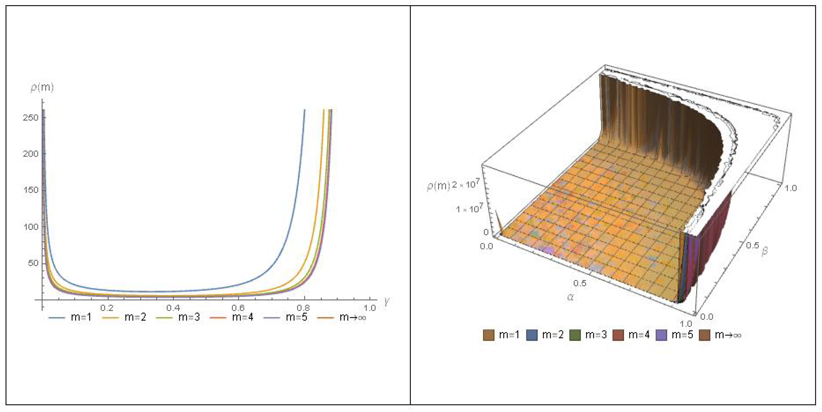
It is easy to see that $\rho \left(m\right)$ is decreasing for all $m\in \mathbb{N}$ which yields that $\rho \left(m\right)<\rho (\infty )$ for all $m\in \mathbb{N}$ and this is obvious also from Figure 1 which also shows that $\rho \left(m\right)$ has maximum values when $\gamma \to 0$ or $\gamma \to 1$ for all $m\in \mathbb{N}\cup \{\infty \}$.

Figure 1. The graph of $\rho \left(m\right)$ at various values of m.

In light of (11), we obtain

$$\begin{array}{c}\hfill \left|B\right|={\left(1-{\displaystyle \frac{{\left(2\rho \right)}^{1-\gamma }(3^m-2^{(1-\gamma )m})}{3^m\mathsf{\Gamma }\left(\gamma \right)(3-2^{1-\gamma })}}\right)}^{-1},m\in \mathbb{N}\end{array}$$

and if $m\to \infty$, we obtain

$$\begin{array}{c}\hfill \left|B\right|={\left(1-{\displaystyle \frac{{\left(2\rho \right)}^{1-\gamma }}{\mathsf{\Gamma }\left(\gamma \right)(3-2^{1-\gamma })}}\right)}^{-1}.\end{array}$$

Inserting the above results into (23) and (24) yield

$$\begin{array}{cc}\hfill R_1& ={\displaystyle \frac{3^m-2^{(1-\alpha -\gamma )m}}{{\left(2\rho \right)}^{\alpha }\mathsf{\Gamma }\left(\alpha +\gamma \right)(3-2^{1-\alpha -\gamma })}}{\left({\displaystyle \frac{3^m}{{\left(2\rho \right)}^{1-\gamma }}}-{\displaystyle \frac{3^m-2^{(1-\gamma )m}}{\mathsf{\Gamma }\left(\gamma \right)(3-2^{1-\gamma })}}\right)}^{-1},m\in \mathbb{N},\hfill \\ \hfill R_2& ={\displaystyle \frac{\mathsf{\Gamma }\left(\gamma \right)}{{\rho }^{\alpha }\mathsf{\Gamma }(\alpha +\gamma )}}.\hfill \end{array}$$

and if $m\to \infty$, we obtain

$$\begin{array}{cc}\hfill R_1& ={\displaystyle \frac{1}{{\left(2\rho \right)}^{\alpha }\mathsf{\Gamma }\left(\alpha +\gamma \right)(3-2^{1-\alpha -\gamma })}}{\left({\displaystyle \frac{1}{{\left(2\rho \right)}^{1-\gamma }}}-{\displaystyle \frac{1}{\mathsf{\Gamma }\left(\gamma \right)(3-2^{1-\gamma })}}\right)}^{-1}.\hfill \end{array}$$

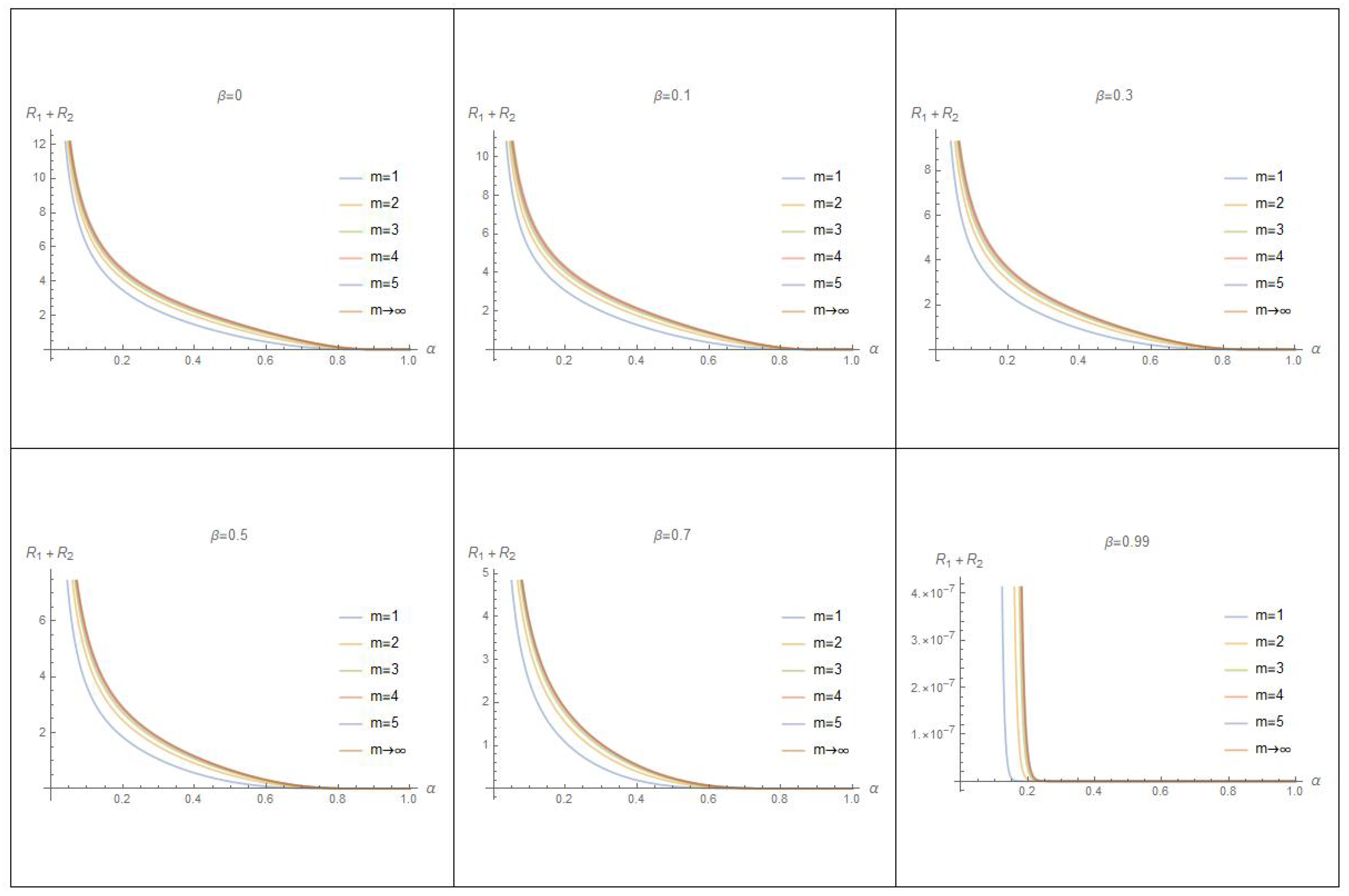
Each graph in Figure 2 shows that the values of $R_1+R_2$ are decreasing by increasing the values of $\alpha$ at various values of m. Also, in view of all graphs in this figure, we note that the maximum value of $R_1+R_2$ is decreasing by increasing the values of $\beta$.

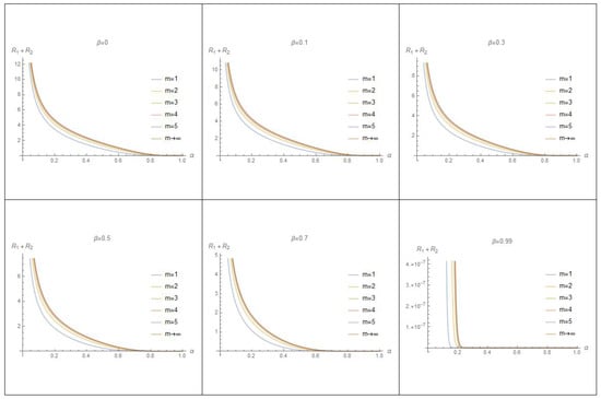
Figure 2. The graph of $R_1+R_2$ at various values of m and $\beta$.

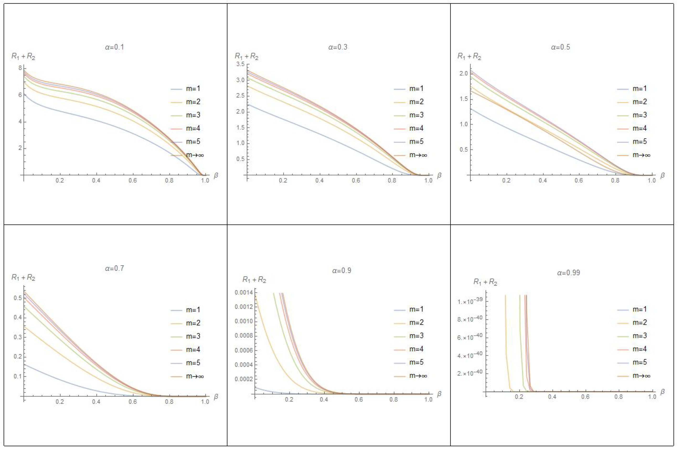
Also, each graph in Figure 3 shows that the values of $R_1+R_2$ are decreasing by increasing the values of $\beta$ at various values of m. Moreover, in view of all graphs in this figure, we note that the maximum value of $R_1+R_2$ is decreasing by increasing the values of $\alpha$.

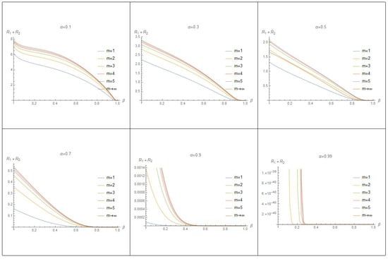
Figure 3. The graph of $R_1+R_2$ at various values of m and $\alpha$.

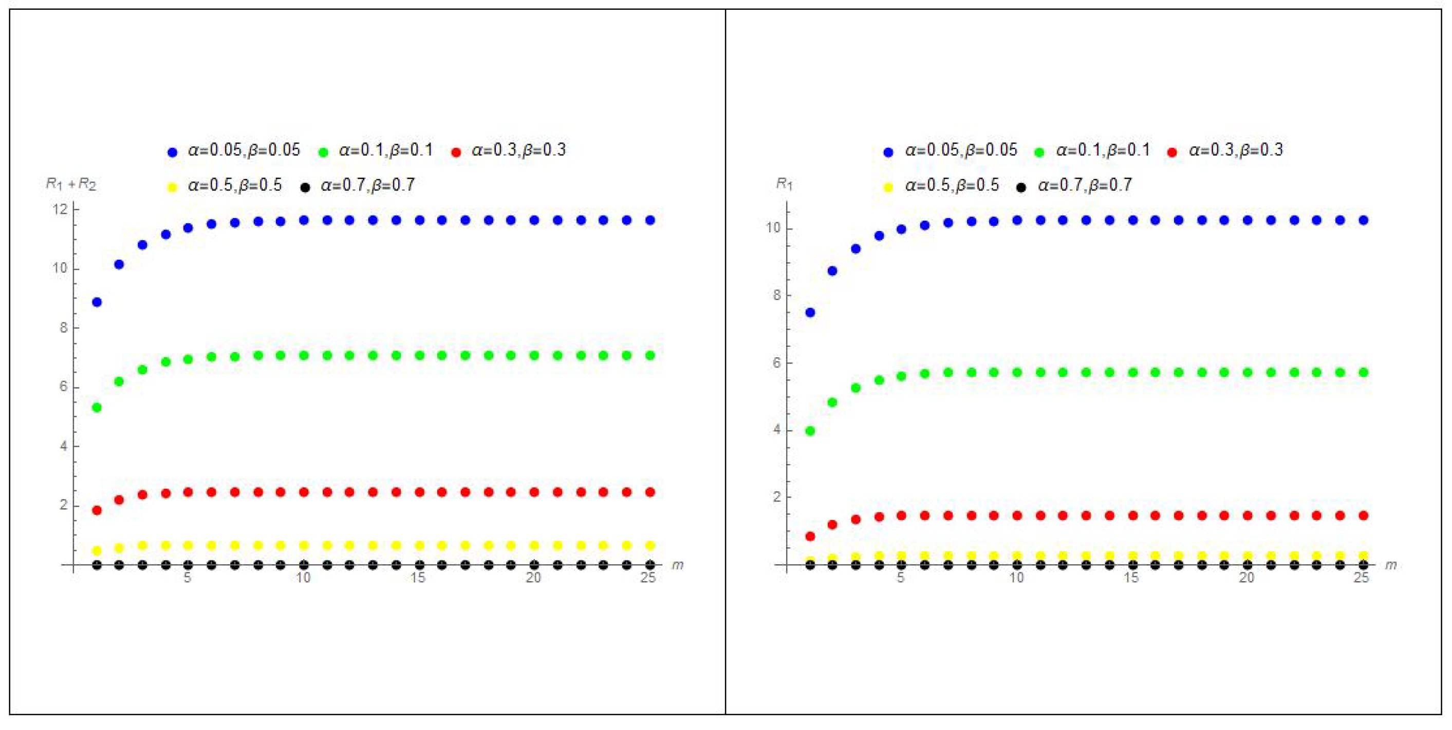
The graphs in Figure 4 show that the values of $R_1+R_2$ and $R_1$ are decreasing by increasing the values of m and increasing the values of $\alpha$ and $\beta$ together.

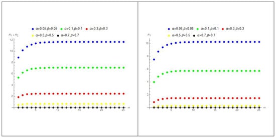
Figure 4. The graph of $R_1+R_2$ at various values of $\alpha$ and $\beta$.

In conclusion, according to Figure 1, Figure 2, Figure 3 and Figure 4, we obtain the maximum value of $R_1+R_2$ and $R_1$ at $m\to \infty$ and sufficiently small of $\alpha$ and $\beta$ together. Therefore, if we take $\alpha =\beta =0.05$ which implies $\gamma =0.0975$, $R_1+R_2=11.6597$ and $R_1=10.2615$. Hence, the control (Bifurcation) parameter $\left|\sigma \right|<1/11.6597\sim 0.0857655\ll 1$ according to Theorem 9 (there exists a unique solution) and $\left|\sigma \right|<1/11.6597\sim 0.0974518\ll 1$ according to Theorem 10 (there exists at least one solution).

7. Conclusions

In conclusion, fractional differential equations are of paramount importance in accurately modeling systems exhibiting memory and hereditary behaviors, extending beyond the limitations of traditional integer-order differential equations. The Hilfer–Katgampola derivatives, as an advanced generalization of fractional derivatives, offer enhanced analytical capabilities for addressing complex systems with nonlocal interactions and memory effects. Collectively, these mathematical tools contribute significantly to the development of more precise and comprehensive models across various scientific disciplines, facilitating a deeper understanding of complex phenomena.

In the context of our research, we relied on two main ideas: The first idea depends on finding the mild solution using semigroup theory and some theorems of Laplace transformation, while the second idea depends on investigating the existence and uniqueness of a mild solution of our fractional evolution equation using some theorem on functional analysis, namely fixed-point theorems.

Finally, we illustrated our results by studying the time fractional Ginzburg–Landau equation, which describes the nonlinear evolution of small disturbances near a finite-wavelength bifurcation from a stable to an unstable state of a system.

References

- Oliver, C. Evolution Equations in Scales of Banach Spaces; TEUBNER-TEXTE zur Mathematik; Springer: Berlin/Heidelberg, Germany, 2002. [Google Scholar]
- Cazenave, T.; Haraux, A.; Martel, Y. An Introduction to Semilinear Evolution Equations; Clarendon Press: Oxford, UK, 1999. [Google Scholar]
- Salem, A.; Alharbi, K.N. Controllability for fractional evolution equations with infinite time-delay and non-local conditions in compact and noncompact cases. Axioms 2023, 12, 264. [Google Scholar] [CrossRef]
- Baghani, H.; Salem, A. Solvability and stability of a class of fractional Langevin differential equations. Boletín Soc. Mat. Mex. 2024, 30, 46. [Google Scholar] [CrossRef]
- Zhou, Y. Basic Theory of Fractional Differential Equations; World Scientific: Singapore, 2014. [Google Scholar]
- Salem, A.; Alharbi, K.N. Fractional infinite time-delay evolution equations with non-instantaneous impulsive. AIMS Math. 2023, 8, 12943–12963. [Google Scholar] [CrossRef]
- Salem, A. Existence results of solutions for anti-periodic fractional Langevin equation. J. Appl. Anal. Comput. 2020, 10, 2557–2574. [Google Scholar] [CrossRef] [PubMed]
- Zhou, Y.; Jiao, F. Existence of mild solutions for fractional neutral evolution equations. Comput. Math. Appl. 2010, 59, 1063–1077. [Google Scholar] [CrossRef]
- Norouzi, F.; N’guérékata, G.M. Existence results to a ψ-Hilfer neutral fractional evolution equation with infinite delay. Nonautonomous Dyn. Syst. 2021, 8, 101–124. [Google Scholar] [CrossRef]
- Suechoei, A.; Ngiamsunthorn, P. Existence uniqueness and stability of mild solutions for semilinear ψ-Caputo fractional evolution equations. Adv. Differ. Equ. 2020, 114, 1–28. [Google Scholar] [CrossRef]
- Salem, A.; Alharbi, K.; Alshehri, H. Fractional Evolution Equations with Infinite Time Delay in Abstract Phase Space. Mathematics 2022, 10, 1332. [Google Scholar] [CrossRef]
- Salem, A.; Alharbi, K.N. Total Controllability for a Class of Fractional Hybrid Neutral Evolution Equations with Non-Instantaneous Impulses. Fractal Fract. 2023, 7, 423. [Google Scholar] [CrossRef]
- Byszewski, L. Theorems about the existence and uniqueness of a semilinar evolution nonlocal Cauchy problem. Math. Anal. Appl. 1991, 162, 494–495. [Google Scholar] [CrossRef]
- Tariboon, J.; Samadi, A.; Ntouyas, S.K. Multi-Point Boundary Value Problems for (k, ϕ)-Hilfer Fractional Differential Equations and Inclusions. Axioms 2022, 11, 110. [Google Scholar] [CrossRef]
- Sevinik-Adigüzel, R.; Aksoy, Ü.; Karapinar, E.; Erhan, I.M. Uniqueness of solution for higher-order nonlinear fractional differential equations with multi-point and integral boundary conditions. Rev. Real Acad. Cienc. Exactas Fís. Nat. Ser. A Mat. 2021, 115, 155. [Google Scholar] [CrossRef]
- Luca, R. Positive Solutions for a System of Fractional q-Difference Equations with Multi-Point Boundary Conditions. Fractal Fract. 2024, 8, 70. [Google Scholar] [CrossRef]
- Salem, A.; Alghamdi, B. Multi-strip and multi-point boundary conditions for fractional Langevin equation. Fractal Fract. 2020, 4, 18. [Google Scholar] [CrossRef]
- Salem, A.; Alghamdi, B. Multi-Point and Anti-Periodic Conditions for Generalized Langevin Equation with Two Fractional Orders. Fractal Fract. 2019, 3, 51. [Google Scholar] [CrossRef]
- Salem, A.; Alzahrani, F.; Alnegga, M. Coupled system of nonlinear fractional Langevin equations with multi-point and nonlocal integral boundary conditions. Math. Probl. Eng. 2020, 2020, 7345658. [Google Scholar] [CrossRef]
- Almaghamsi, L.; Salem, A. Fractional Langevin equations with infinite-point boundary condition: Application to Fractional harmonic oscillator. J. Appl. Anal. Comput. 2023, 13, 3504–3523. [Google Scholar] [CrossRef]
- Deng, K. Exponential Decay of Solutions of Semilinear Parabolic Equations with Nonlocal Initial Conditions. J. Math. Anal. Appl. 1993, 179, 630–637. [Google Scholar] [CrossRef]
- Ginzburg, V.L.; Landau, L.D. On the Theory of Superconductivity. Zhurnal Eksperimental’noi Teor. Fiz. 1950, 20, 1064–1082. [Google Scholar]
- Newell, A.C.; Whitehead, J.A. Finite bandwidth, finite amplitude convection. J. Fluid Mech. 1969, 38, 279–303. [Google Scholar] [CrossRef]
- Segel, A.L. Distant side-walls cause slow amplitude modulation of cellular convection. J. Fluid Mech. 1969, 38, 203–224. [Google Scholar] [CrossRef]
- Raza, N. Exact periodic and explicit solutions of the conformable time fractional Ginzburg Landau equation. Opt. Quant. Electron. 2018, 50, 154. [Google Scholar] [CrossRef]
- Akram, G.; Arshed, S.; Sadaf, M.; Farooq, K. A study of variation in dynamical behavior of fractional complex Ginzburg-Landau model for different fractional operators. Ain Shams Eng. J. 2023, 14, 102120. [Google Scholar] [CrossRef]
- Murad, M.A.S.; Ismael, H.F.; Hamasalh, F.K.; Shah, N.A.; Eldin, S.M. Optical soliton solutions for time-fractional Ginzburg-Landau equation by a modified sub-equation method. Results Phys. 2023, 53, 106950. [Google Scholar] [CrossRef]
- Zhou, Y. Fractional Evolution Equations and Inclusions; Academic Press: Cambridge, MA, USA, 2016. [Google Scholar]
- Jiménez, V.M.; de León, M. The evolution equation: An application of groupoids to material evolution. J. Geom. Mech. 2022, 14, 331–348. [Google Scholar] [CrossRef]
- Salem, A.; Abdullah, S. Controllability results to non-instantaneous impulsive with infinite delay for generalized fractional differential equations. Alex. Eng. J. 2023, 70, 525–533. [Google Scholar] [CrossRef]
- Jarad, F.; Abdeljawad, T. A modified Laplace transform for certain generalized fractional operators. Results Nonlinear Anal. 2018, 1, 88–98. [Google Scholar]
- Katugampola, U. New approach to a generalized fractional integral. Appl. Math. Comput. 2011, 218, 860–865. [Google Scholar] [CrossRef]
- Katugampola, U. New approach to a generalized fractional derivatives. Bull. Math. Anal. Appl. 2014, 6, 1–15. [Google Scholar]
- Oliveira, D.; de Oliveira, E.C. Hilfer-Katugampola fractional derivatives. Comp. Appl. Math. 2018, 37, 3672–3690. [Google Scholar] [CrossRef]
- Hong, D.; Wang, J.; Gardner, R. Real Analysis with an Introduction to Wavelets; Elsevier Inc.: London, UK, 2005. [Google Scholar]
- Lundsgaard, H.V. Functional Analysis Entering Hilbert Space, 2nd ed.; World Scientific: Singapore, 2006. [Google Scholar]
- Almeida, R. A Gronwall inequality for a general Caputo fractional operator. Math. Inequalities Appl. 2017, 20, 1089–1105. [Google Scholar] [CrossRef]
- Abdeljawad, T. On conformable fractional calculus. J. Compubtational Appl. Math. 2013, 279, 57–66. [Google Scholar] [CrossRef]
- Pazy, A. Semigroups of Linear Operators and Applications to Partial Differential Equations, 1st ed.; Springer New York Inc.: New York, NY, USA, 1983. [Google Scholar]
Disclaimer/Publisher’s Note: The statements, opinions and data contained in all publications are solely those of the individual author(s) and contributor(s) and not of MDPI and/or the editor(s). MDPI and/or the editor(s) disclaim responsibility for any injury to people or property resulting from any ideas, methods, instructions or products referred to in the content. |
© 2025 by the authors. Licensee MDPI, Basel, Switzerland. This article is an open access article distributed under the terms and conditions of the Creative Commons Attribution (CC BY) license (https://creativecommons.org/licenses/by/4.0/).