A Quasi-Explicit Method Applied to Missing Boundary Data Reconstruction for the Stokes System

Abstract

In this paper, we study the data completion problem for the Cauchy–Stokes equation in a cylindrical domain, $\mathsf{\Omega }$. Neumann and Dirichlet boundary conditions are prescribed on part of the overdetermined boundary, ${\mathsf{\Gamma }}_0$, and the goal is to complete the data on the other part of the boundary, ${\mathsf{\Gamma }}_a$. Here, ${\mathsf{\Gamma }}_0$ and ${\mathsf{\Gamma }}_a$ represent the side faces of the cylinder $\mathsf{\Omega }$. This problem is known to be ill-posed and is formulated as an optimal control problem with a regularized cost function. To directly approximate the missing data on ${\mathsf{\Gamma }}_a$, we employ the method of factorization of elliptic boundary value problems. This technique allows the factorization of a boundary value problem into a product of parabolic problems. It is successfully applied to the optimality system in this work, yielding new and significant results.

1. Introduction

Completing the Navier–Stokes equations’ missing boundary data is a crucial task in many engineering and scientific fields. When predicting the weather and modeling the climate for accurate weather and climate forecasts, accurate simulations of oceanic and atmospheric circulation are necessary. However, measurements of boundary conditions, including the temperature gradients, pressure, and wind velocity, are frequently lacking. Refining the numerical models employed in projections requires us to fill this data gap (see [1,2]). Measurement method limitations might result in incomplete boundary data in engineering domains such as hydrodynamics and aerodynamics. For example, not all boundary conditions are understood in detail for wind tunnel studies. When these missing data are filled in, accurate simulations are guaranteed, which is essential in developing effective systems like turbines, cars, and airplanes (see [3]). In the field of biomedical engineering, when simulating physiological flows like blood circulation in arteries or respiratory system airflow, one frequently encounters unidentified boundary conditions like pressure or wall shear stress. By filling in these missing data, the simulations are improved and medical devices like artificial valves and stents can be designed more effectively [4]. In environmental engineering, the modeling of water flows in natural settings, such as rivers, lakes, or coastal regions, often involves inaccessible areas where boundary data are missing. Completing these data is essential in simulating pollutant dispersion, sediment transport, and flood dynamics, thereby informing environmental management and disaster preparedness; see [5].

In applications such as drag reduction in aerodynamics or mixing enhancement in chemical reactors, missing boundary data present significant challenges for active flow control. Resolving this issue is essential in designing effective control strategies that optimize system performance; see [6].

The problem of missing boundary data is often addressed using inverse problems, where unknown boundary conditions are inferred from available measurements. Techniques such as data assimilation, regularization methods, and physics-informed neural networks are commonly employed to reconstruct the missing information, ensuring accurate and reliable simulations.

For example, in the context of the Navier–Stokes equations, stability estimates have been utilized in inverse problems to recover boundary coefficients from measurements. These approaches are critical in ensuring the accuracy and reliability of simulations across a range of applications.

In summary, completing missing boundary data in the Navier–Stokes equations is fundamental for accurate modeling and simulation in various fields, including weather forecasting, industrial design, biomedical engineering, environmental management, and fluid system optimization.

This work focuses on the Cauchy–Stokes problem within a cylindrical domain $\mathsf{\Omega }$, where data are provided on a portion of $\mathsf{\Omega }$’s boundary. Notably, there is limited literature on the Cauchy–Stokes problem. For instance, ref. [7] addresses this issue by modeling the data recovery process as a least-squares tracking problem. Moreover, alternating iterative algorithms have been applied in [8,9] for elliptic equations and in [10,11,12,13] for stationary Stokes systems. The Poincaré–Steklov operator is employed in [14] as another method to tackle this problem.

In this paper, we present the factorization method, which reformulates the elliptic boundary value problem as a parabolic one. This technique provides a direct means of computing the missing boundary data for any specified Cauchy data.

This technique consists of embedding the initial problem in a family of similar problems depending on a parameter, and these are solved recursively. It can be viewed as an infinite-dimensional generalization of the block Gauss LU factorization. It has been used by Bellman [15] and Lions [16] (in the infinite-dimensional case) to derive the optimal feedback law in linear-quadratic optimal control problems. The method applied to the Poisson equation has been presented in [17,18], and it has recently been used by Bouarroudj et al. in [19,20] to analyze boundary-value problems for fourth-order partial differential equations Moreover, it has already been used to solve the electrocardiographic imaging (ECGI) problem in the work by Addouche et al. [21]. The Cauchy–Stokes systems have been presented in [22], which are the same as in [23,24]. Moreover, we have Dirichlet and Neumann data on the whole boundary of $\mathsf{\Omega }$ (see Figure 1), and we search for the speed and the pressure in $\mathsf{\Omega }$. This problem is well-posed and has a unique weak solution. In our work, we solve an inverse problem: a data completion problem for the Stokes equation in $\mathsf{\Omega }$. The velocity $\mathcal{U}$ (a Dirichlet datum) and a force $\mathcal{F}$ are given on part of the boundary of $\mathsf{\Omega }$, accessible via direct measurement, while no condition is given on ${\mathsf{\Gamma }}_a$ (inaccessible via direct measurements). The data completion problem consists of recovering a boundary condition on ${\mathsf{\Gamma }}_a$ to directly obtain an approximation of the missing data. This problem is known to be severely ill-posed (see Hadamard [25]); it is set as an optimal control problem with a cost function.

Figure 1. Schematic representation of the cylindrical domain $\mathsf{\Omega }$.

This paper is organized as follows. In Section 2, we introduce the cylindrical geometry of the domain $\mathsf{\Omega }$ and establish key notations, Sobolev spaces, and the forward Stokes problem. The inverse problem is then rigorously formulated as a Cauchy–Stokes data completion task. Section 3 transforms this ill-posed inverse problem into a well-posed optimal control framework, defining the energy-like error functional and proving its convexity. Section 4 presents the core theoretical advancements, including the factorization method’s application to derive decoupled Riccati equations for the Dirichlet-to-Neumann (D) and Neumann-to-Dirichlet (Q) operators, alongside critical theorems governing the optimality system. Section 5 provides the detailed proof of Theorem 1, elucidating the structure and evolution of the operator D. In Section 6, we solve the optimal control problem non-iteratively using the factorization method, proving Theorems 2 and 3 to characterize the missing boundary data and establish compatibility conditions. Finally, Section 7 concludes with insights into the method’s efficiency, numerical prospects, and extensions to non-cylindrical domains. This revised structure emphasizes the interplay between theoretical analysis and computational strategy, offering a cohesive pathway from problem formulation to solution.

2. Preliminaries

2.1. Notations

Let $\mathsf{\Omega }$ be the open-bounded cylinder $\mathsf{\Omega }=\left]0,a\right[\times \mathcal{O}$ in ${\mathbb{R}}^n$, where $a>0$, and $\mathcal{O}$ is a bounded open set in ${\mathbb{R}}^{n-1}$, representing the cross-section of the cylinder. Let $\mathsf{\Sigma }=\left]0,a\right[\times \partial \mathcal{O}$ denote the lateral boundary and ${\mathsf{\Gamma }}_0=\left\{0\right\}\times \mathcal{O}$ and ${\mathsf{\Gamma }}_a=\left\{a\right\}\times \mathcal{O}$ be the faces of the cylinder. A general point $(x_1,x_2,\dots ,x_n)$ is also denoted by $(x,\mathbf{y})$, where $x=x_1$ is the coordinate along the axis of the cylinder, and $\mathbf{y}=(x_2,\dots ,x_n)$ represents the coordinates in the cross-section, perpendicular to the axis. The cylindrical geometry simplifies the presentation of the factorization method, but the method can be easily generalized to regular non-cylindrical domains.

Firstly, to emphasize the role of the component along the axis of the cylinder, which will play a crucial role in the factorization method, we introduce the following notations.

• For a given vector field $\mathsf{\Theta }$, we denote by ${\mathsf{\Theta }}_x$ the component of $\mathsf{\Theta }$ along the axis of the cylinder and by ${\mathsf{\Theta }}_{\mathbf{y}}$ its components with respect to the coordinates in the cross-section.
• ∇ represents the gradient vector, where ${\nabla }_x={\displaystyle \frac{\partial }{\partial x_1}}$, and ${\nabla }_{\mathbf{y}}$ denotes the components with respect to the coordinates in the cross-section.
• For a given vector field $\mathsf{\Theta }$, we define the divergence as

  $$div\left(\mathsf{\Theta }\right)=\sum _{i=1}^n{\displaystyle \frac{\partial \mathsf{\Theta }}{\partial x_i}},$$

  with

  $$di{v}_x\left(\mathsf{\Theta }\right)={\displaystyle \frac{\partial \mathsf{\Theta }}{\partial x_1}},di{v}_{\mathbf{y}}\left(\mathsf{\Theta }\right)=\sum _{i=2}^n{\displaystyle \frac{\partial \mathsf{\Theta }}{\partial x_i}}.$$

Secondly, we introduce the following notations.

• $\nu$ represents the fluid kinematic viscosity.
• The strain tensor is given by

  $$T\left(\mathbf{u}\right)={\displaystyle \frac{1}{2}}(\nabla \mathbf{u}+{(\nabla \mathbf{u})}^t),$$

  where

  $${\left(T\left(\mathbf{u}\right)\right)}_{ij}={\displaystyle \frac{1}{2}}\left({\displaystyle \frac{\partial {\mathbf{u}}_{x_i}}{\partial x_j}}+{\displaystyle \frac{\partial {\mathbf{u}}_{x_j}}{\partial x_i}}\right),1\le i,j\le n.$$
• The stress tensor is defined as

  $$\sigma \left(\mathbf{u}\right)=2\nu T\left(\mathbf{u}\right)-pI.$$
• I denotes the identity matrix.
• N is the outward unit normal vector; in our case, $N=(-1,0,\dots ,0)$ on ${\mathsf{\Gamma }}_0$ and $N=(1,0,\dots ,0)$ on ${\mathsf{\Gamma }}_a$.
• We denote by $\nabla \mathbf{u}:\nabla v$ the trace of their product, which is defined as

  $$\nabla \mathbf{u}:\nabla v=tr(\nabla \mathbf{u}\nabla v)=\sum _{i=1}^n\nabla u_{x_i}\nabla v_{x_i}=\sum _{i,j=1}^n{\displaystyle \frac{\partial u_{x_i}}{\partial x_j}}{\displaystyle \frac{\partial v_{x_j}}{\partial x_i}},$$

  where

  $$\nabla \mathbf{u}=\left(\begin{array}{c}\nabla u_{x_1}\\ ⋮\\ \nabla u_{x_n}\end{array}\right)=\left(\begin{array}{ccc}{\displaystyle \frac{\partial u_{x_1}}{\partial x_1}}& \cdots & {\displaystyle \frac{\partial u_{x_1}}{\partial x_n}}\\ ⋮& \ddots & ⋮\\ {\displaystyle \frac{\partial u_{x_n}}{\partial x_1}}& \cdots & {\displaystyle \frac{\partial u_{x_n}}{\partial x_n}}\end{array}\right).$$
  The Laplacian of $\mathbf{u}$ is given by

  $$\Delta \mathbf{u}=\left(\begin{array}{c}\Delta u_{x_1}\\ ⋮\\ \Delta u_{x_n}\end{array}\right).$$

Finally, we define the following Sobolev space.

• The Sobolev space $H_{00}^{1/2}\left(\mathcal{O}\right)$ is defined, as stated in Theorem 11.7 (p. 72) of [16], as the ${\displaystyle \frac{1}{2}}$-interpolation between $H_0^1\left(\mathcal{O}\right)$ and $L^2\left(\mathcal{O}\right)$. Its dual space is denoted by ${\left(H_{00}^{1/2}\left(\mathcal{O}\right)\right)}^{\prime }$.

2.2. Forward Problem

The direct problem is defined as follows: for a given $\mathcal{U}\in H_{00}^{1/2}\left({\mathsf{\Gamma }}_0\right)$ and $\mathcal{G}\in {\left(H_{00}^{1/2}\left({\mathsf{\Gamma }}_a\right)\right)}^{\prime }$, find the velocity $\mathbf{u}\in H^1\left(\mathsf{\Omega }\right)$ and the pressure $p\in L^2\left(\mathsf{\Omega }\right)$ satisfying

$$\left(\mathcal{P}\right)\left\{\begin{array}{cc}-\nu \Delta \mathbf{u}+\nabla p=0\hfill & \mathrm{in}\mathsf{\Omega },\hfill \\ div\left(\mathbf{u}\right)=0\hfill & \mathrm{in}\mathsf{\Omega },\hfill \\ \mathbf{u}=0\hfill & \mathrm{on}\mathsf{\Sigma },\hfill \\ \mathbf{u}=\mathcal{U}\hfill & \mathrm{on}{\mathsf{\Gamma }}_0,\hfill \\ \sigma \left(\mathbf{u}\right)·N=\mathcal{G}\hfill & \mathrm{on}{\mathsf{\Gamma }}_a.\hfill \end{array}\right.$$

(1)

Physical Interpretation

In Problem $\left(\mathcal{P}\right)$ (Equation (1)), the unknowns $\mathbf{u}$ and p represent the following.

• Velocity field ($\mathbf{u}$): $\mathbf{u}\in H^1\left(\mathsf{\Omega }\right)$ describes the fluid motion in $\mathsf{\Omega }$, satisfying the following:

  –

  No-slip condition, $\mathbf{u}=0$ on $\mathsf{\Sigma }$;

  –

  Prescribed velocity, $\mathbf{u}=\mathcal{U}$ on ${\mathsf{\Gamma }}_0$;

  –

  Traction condition, $\sigma \left(\mathbf{u}\right)·N=\mathcal{G}$ on ${\mathsf{\Gamma }}_a$.

• Pressure field (p): $p\in L^2\left(\mathsf{\Omega }\right)$ enforces incompressibility ($\mathrm{div}\left(\mathbf{u}\right)=0$) and balances viscous forces through $\nabla p$.

We need the following lemma that provides a general integration by parts formula.

Lemma 1

([14,26]). If $\mathit{u}\in H^1\left(\mathsf{\Omega }\right),$ such that $div\left(\mathit{u}\right)=0$ in Ω, then $\Delta \mathit{u}=2\nabla ·T\left(\mathit{u}\right)$ and

$$-{\int }_{\mathsf{\Omega }}\nu \Delta \mathit{u}·vdx={\int }_{\mathsf{\Omega }}2\nu T\left(\mathit{u}\right):T\left(v\right)dx-{\int }_{\partial \mathsf{\Omega }}2\nu T\left(\mathit{u}\right)N·vdx,\mathit{for}\mathit{all}v\in H^1\left(\mathsf{\Omega }\right).$$

Let the space $Y=\left\{\mathbf{u}\in H^1\left(\mathsf{\Omega }\right):div\left(\mathbf{u}\right)=0\mathrm{and}\mathsf{\Omega },\mathbf{u}=0\mathrm{on}\mathsf{\Sigma }\cup {\mathsf{\Gamma }}_0\right\}$. Then, a mixed formulation of the Stokes equations is obtained by multiplying the first equation of $\left(\mathcal{P}\right)$ by a test function $v\in Y,$ by integration over $\mathsf{\Omega },$ and by applying Lemma 1 as well as the divergence theorem. Then,

$${\int }_{\mathsf{\Omega }}2\nu T\left(\mathbf{u}\right):T\left(v\right)dx-{\int }_{\mathsf{\Omega }}pdiv\left(v\right)dx={\int }_{\partial \mathsf{\Omega }}\left(2\nu T\left(\mathbf{u}\right)N\right)·vdx-{\int }_{\partial \mathsf{\Omega }}\left(pN\right)vdx.$$

Using the boundary conditions where $\mathbf{u}\in Y$ satisfies the constraint ${\mathbf{u}}_{\mid {\mathsf{\Gamma }}_0}=\mathcal{U}$, we obtain

$$\begin{array}{ccc}\hfill {\int }_{\mathsf{\Omega }}2\nu T\left(\mathbf{u}\right):T\left(v\right)dx& =& {\int }_{\partial \mathsf{\Omega }}(2\nu T\left(\mathbf{u}\right)-p)N·vdx\hfill \\ & =& {\int }_{{\mathsf{\Gamma }}_a}(2\nu T\left(\mathbf{u}\right)-p)N·vdx\hfill \\ & =& {\int }_{{\mathsf{\Gamma }}_a}\mathcal{G}vdx.\hfill \end{array}$$

We write, for all $(\mathbf{u},v)\in Y\times Y,$

$$a(\mathbf{u},v)={\int }_{\mathsf{\Omega }}2\nu T\left(\mathbf{u}\right):T\left(v\right)dx\mathrm{and}l\left(v\right)={\int }_{{\mathsf{\Gamma }}_a}\mathcal{G}vdx.$$

So, $\mathbf{u}$ is a weak solution of $\left(\mathcal{P}\right)$ if and only if $a(\mathbf{u},v)-l\left(v\right)=0,$ for all $v\in Y$.

The well-posedness of the above variational formulation is given by the Lax–Milgram theorem (see [16] for more details).

2.3. The Inverse Problem

Assuming a given velocity $\mathcal{U}\in H_{00}^{1/2}\left({\mathsf{\Gamma }}_0\right)$ and a force $\mathcal{F}\in {\left(H_{00}^{1/2}\left({\mathsf{\Gamma }}_0\right)\right)}^{\prime }$ on ${\mathsf{\Gamma }}_0$, the data completion problem for the Stokes operator can be formulated as a Cauchy problem.

Find the velocity $\mathbf{u}\in \mathcal{H}$ and the pressure $p\in \mathcal{P}$ satisfying

$$\left(\mathcal{PI}\right)\left\{\begin{array}{cc}-\nu \Delta \mathbf{u}+\nabla p=0\hfill & \mathrm{in}\mathsf{\Omega },\hfill \\ div\left(\mathbf{u}\right)=0\hfill & \mathrm{in}\mathsf{\Omega },\hfill \\ \mathbf{u}=0\hfill & \mathrm{on}\mathsf{\Sigma },\hfill \\ \mathbf{u}=\mathcal{U}\hfill & \mathrm{on}{\mathsf{\Gamma }}_0,\hfill \\ \sigma \left(\mathbf{u}\right)·N=\mathcal{F}\hfill & \mathrm{on}{\mathsf{\Gamma }}_0.\hfill \end{array}\right.$$

(2)

We have on ${\mathsf{\Gamma }}_0$

$$\sigma \left(\mathbf{u}\right)·N=\mathcal{F}\mathrm{on}{\mathsf{\Gamma }}_0\Rightarrow \left\{\begin{array}{cc}p\left(0\right)-2\nu {\displaystyle \frac{\partial u_{x_1}}{\partial x_1}}\left(0\right)={\mathcal{F}}_{x_1},\hfill & \\ -\nu ({\displaystyle \frac{\partial u_{x_j}}{\partial x_1}}\left(0\right)+{\displaystyle \frac{\partial u_{x_1}}{\partial x_j}}\left(0\right))={\mathcal{F}}_{x_j},j=2,\dots ,n.\hfill \end{array}\right.$$

This can be expressed as follows:

$$\begin{array}{ccc}p\left(0\right)-2\nu {\displaystyle \frac{\partial u_x}{\partial x}}\left(0\right)={\mathcal{F}}_x,\hfill & \hfill & \\ -\nu ({\displaystyle \frac{\partial {\mathbf{u}}_{\mathbf{y}}}{\partial x}}\left(0\right)+\left({\nabla }_{\mathbf{y}}\right)u_x\left(0\right))={\mathcal{F}}_{\mathbf{y}},\hfill & \hfill \end{array}$$

(3)

where ${\nabla }_{\mathbf{y}}={({\partial }_{x_2},\dots ,{\partial }_{x_n})}^t$ is the gradient operator defined on the section of the cylinder; $u_x=u_{x_1}$ and ${\mathbf{u}}_{\mathbf{y}}={(u_{x_2},\dots ,u_{x_n})}^t$ are the components of the vector u.

This problem is known to be ill-posed in the sense that the dependence of $(\mathbf{u},p)$ on the data $(\mathcal{U},\mathcal{F})$ is not continuous and the solution does not exist for any pair of data; see [25].

The Cauchy data $(\mathcal{U},\mathcal{F})$ are called compatible if the problem (2) has a solution.

In order to reconstruct the unknown boundary data ${\mathbf{u}}_{|{\mathsf{\Gamma }}_a}$ and $\sigma \left(\mathbf{u}\right)·N_{|{\mathsf{\Gamma }}_a}$ on ${\mathsf{\Gamma }}_a,$ we will use the factorization method (see [27,28,29] for the Laplace equation). The inverse problem is formulated as an optimization one.

2.4. Data Completion Problem

The considered data completion problem $\left({\mathcal{P}}_0\right)$ can be stated as follows: for given compatible data $(\mathcal{U},\mathcal{F})\in H_{00}^{1/2}\left({\mathsf{\Gamma }}_0\right)\times {\left(H_{00}^{1/2}\left({\mathsf{\Gamma }}_0\right)\right)}^{\prime }$, for which the existence and uniqueness of the solution are guaranteed, find the unknown boundary data $(V,G)\in H_{00}^{1/2}\left({\mathsf{\Gamma }}_a\right)\times {\left(H_{00}^{1/2}\left({\mathsf{\Gamma }}_a\right)\right)}^{\prime }$ such that

$$\left({\mathcal{P}}_0\right)\left\{\begin{array}{cc}-\nu \Delta \mathbf{u}+\nabla p=0\hfill & \mathrm{in}\mathsf{\Omega },\hfill \\ div\left(\mathbf{u}\right)=0\hfill & \mathrm{in}\mathsf{\Omega },\hfill \\ \mathbf{u}=0\hfill & \mathrm{on}\mathsf{\Sigma },\hfill \\ \mathbf{u}=\mathcal{U}\hfill & \mathrm{on}{\mathsf{\Gamma }}_0,\hfill \\ \sigma \left(\mathbf{u}\right)·N=\mathcal{F}\hfill & \mathrm{on}{\mathsf{\Gamma }}_0,\hfill \\ \mathbf{u}=V\hfill & \mathrm{on}{\mathsf{\Gamma }}_a,\hfill \\ \sigma \left(\mathbf{u}\right)·N=G\hfill & \mathrm{on}{\mathsf{\Gamma }}_a.\hfill \end{array}\right.$$

(4)

To solve this problem, the unknown data $(V,G)$ will be characterized as the minimum of an energy-like functional; see [8,30,31].

2.5. Optimal Control Problem

The data completion problem $\left({\mathcal{P}}_0\right)$ is transformed into an optimal control problem following the approach used in [8]. It has two states and translates into the two following Stokes problems. Find ${\mathbf{u}}^N$ and ${\mathbf{u}}^D$ solutions of

$$\left({\mathcal{P}}_1\right)\left\{\begin{array}{cc}-\nu \Delta {\mathbf{u}}^N+\nabla p^N=0\hfill & \mathrm{in}\mathsf{\Omega },\hfill \\ div\left({\mathbf{u}}^N\right)=0\hfill & \mathrm{in}\mathsf{\Omega },\hfill \\ {\mathbf{u}}^N=0\hfill & \mathrm{on}\mathsf{\Sigma },\hfill \\ \sigma \left({\mathbf{u}}^N\right)·N=\mathcal{F}\hfill & \mathrm{on}{\mathsf{\Gamma }}_0,\hfill \\ {\mathbf{u}}^N=v\hfill & \mathrm{on}{\mathsf{\Gamma }}_a.\hfill \end{array}\right.$$

$$\left({\mathcal{P}}_2\right)\left\{\begin{array}{cc}-\nu \Delta {\mathbf{u}}^D+\nabla p^D=0\hfill & \mathrm{in}\mathsf{\Omega },\hfill \\ div\left({\mathbf{u}}^D\right)=0\hfill & \mathrm{in}\mathsf{\Omega },\hfill \\ {\mathbf{u}}^D=0\hfill & \mathrm{on}\mathsf{\Sigma },\hfill \\ {\mathbf{u}}^D=\mathcal{U}\hfill & \mathrm{on}{\mathsf{\Gamma }}_0,\hfill \\ \sigma \left({\mathbf{u}}^D\right)·N=g\hfill & \mathrm{on}{\mathsf{\Gamma }}_a.\hfill \end{array}\right.$$

The unknown data $(V,G)$ appearing in the problem $\left({\mathcal{P}}_0\right)$ can be characterized as the solution of the following minimization problem:

$$(V,G)=argmin\left\{E(v,g);(v,g)\in U_{ad}\right\}$$

where E is the following energy-like error functional defined on $U_{ad}=\left(H_{00}^{1/2}\left(\mathcal{O}\right)\right)\times {\left(H_{00}^{1/2}\left(\mathcal{O}\right)\right)}^{\prime }$ by

$$E(v,g)={\displaystyle \frac{1}{2}}{\int }_{\mathsf{\Omega }}\sigma ({\mathbf{u}}^N\left(v\right)-{\mathbf{u}}^D\left(g\right)):\nabla ({\mathbf{u}}^N\left(v\right)-{\mathbf{u}}^D\left(g\right))dx.$$

(5)

Lemma 2.

The functional E defined by Equation (5) is an energy functional that is positive, and, if $\mathcal{U}$ and $\mathcal{F}$ are compatible, then there exists a unique solution that is the minimum of the functional E.

$$E(v,g)={\displaystyle \frac{1}{2}}{\int }_{\mathsf{\Omega }}\sigma ({\mathbf{u}}^N\left(v\right)-{\mathbf{u}}^D\left(g\right)):\nabla ({\mathbf{u}}^N\left(v\right)-{\mathbf{u}}^D\left(g\right))dx.$$

We write $\tilde{u}=({\mathbf{u}}^N\left(v\right)-{\mathbf{u}}^D\left(g\right))dx$ and $\tilde{p}=p^N-p^D$.

Then,

$$\begin{array}{ccc}\hfill E(v,g)& =& {\displaystyle \frac{1}{2}}{\int }_{\mathsf{\Omega }}\sigma \left(\tilde{u}\right):\nabla \left(\tilde{u}\right)dx\hfill \\ & =& {\displaystyle \frac{1}{2}}{\int }_{\mathsf{\Omega }}(\nabla \tilde{u}+{(\nabla \tilde{u})}^t-\tilde{p}I):\nabla \tilde{u}dx\hfill \\ & =& {\displaystyle \frac{1}{2}}{\int }_{\mathsf{\Omega }}(\nabla \tilde{u}:\nabla \tilde{u}+{(\nabla \tilde{u})}^t:\nabla \tilde{u}-\underset{0}{\underbrace{\tilde{p}div\tilde{u}}}dx\hfill \\ & =& {\displaystyle \frac{1}{2}}{\int }_{\mathsf{\Omega }}\sum _{i,j=1}^n\left({\displaystyle \frac{\partial {\tilde{u}}_{x_i}}{\partial x_j}}{\displaystyle \frac{\partial {\tilde{u}}_{x_j}}{\partial x_i}}+{\left({\displaystyle \frac{\partial {\tilde{u}}_{x_i}}{\partial x_j}}\right)}^2\right)dx.\hfill \end{array}$$

We have

$$\begin{array}{ccc}\hfill \sum _{i,j=1}^n{\left({\displaystyle \frac{\partial {\tilde{u}}_{x_i}}{\partial x_j}}+{\displaystyle \frac{\partial {\tilde{u}}_{x_j}}{\partial x_i}}\right)}^2& =& \sum _{i,j=1}^n{\left({\displaystyle \frac{\partial {\tilde{u}}_{x_i}}{\partial x_j}}\right)}^2+{\left({\displaystyle \frac{\partial {\tilde{u}}_{x_j}}{\partial x_i}}\right)}^2+2{\displaystyle \frac{\partial {\tilde{u}}_{x_i}}{\partial x_j}}{\displaystyle \frac{\partial {\tilde{u}}_{x_j}}{\partial x_i}}\hfill \\ & =& 2\left(\sum _{i,j=1}^n{\left({\displaystyle \frac{\partial {\tilde{u}}_{x_i}}{\partial x_j}}\right)}^2+{\displaystyle \frac{\partial {\tilde{u}}_{x_i}}{\partial x_j}}{\displaystyle \frac{\partial {\tilde{u}}_{x_j}}{\partial x_i}}\right),\hfill \end{array}$$

and then

$$E(v,g)={\displaystyle \frac{1}{4}}{\int }_{\mathsf{\Omega }}\sum _{i,j=1}^n{\left({\displaystyle \frac{\partial {\tilde{u}}_{x_i}}{\partial x_j}}+{\displaystyle \frac{\partial {\tilde{u}}_{x_j}}{\partial x_i}}\right)}^{2}dx.$$

So, $E(v,g)$ is positive energy. For the existence of a minimum of E when $(U,F)$ is a compatible pair, see [14].

3. Brief Sketch of the Factorization Method

In this section, we apply the factorization method to the states ${\mathbf{u}}^N$, ${\mathbf{u}}^D.$ We embed the control problem in a family of similar problems defined on the ${\mathsf{\Omega }}_s$ subdomain of $\mathsf{\Omega }$. For this, we define ${\mathsf{\Gamma }}_s=\left\{x=s\right\}\times \mathcal{O}$ as a mobile border that will move from $x=0$ to $x=a$. At each position $x=s$, one can thus define a subdomain ${\mathsf{\Omega }}_s$ of surface side ${\mathsf{\Sigma }}_s$ delimited by surfaces ${\mathsf{\Gamma }}_0$ and ${\mathsf{\Gamma }}_s$ (see Figure 2).

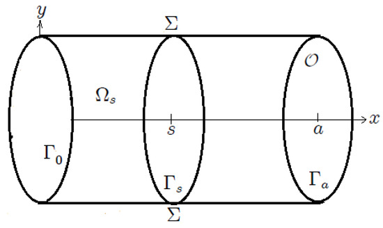
Figure 2. Schematic representation of the moving domain ${\mathsf{\Omega }}_s$.

For given boundary data $(\psi ,\phi )\in H_{00}^{1/2}\left({\mathsf{\Gamma }}_s\right)\times {\left(H_{00}^{1/2}\left({\mathsf{\Gamma }}_s\right)\right)}^{\prime }$, we define ${\mathbf{u}}^{N_s}$ and ${\mathbf{u}}^{D_s}$ as the solutions to the following two problems in ${\mathsf{\Omega }}_s$:

$$\left({\mathcal{P}}_1^s\right)\left\{\begin{array}{cc}-\nu \Delta {\mathbf{u}}^{N_s}+\nabla p^{N_s}=0\hfill & \mathrm{in}{\mathsf{\Omega }}_s,\hfill \\ div\left({\mathbf{u}}^{N_s}\right)=0\hfill & \mathrm{in}{\mathsf{\Omega }}_s,\hfill \\ {\mathbf{u}}^{N_s}=0\hfill & \mathrm{on}{\mathsf{\Sigma }}_s,\hfill \\ {\mathbf{u}}^{N_s}=\psi \hfill & \mathrm{on}{\mathsf{\Gamma }}_s,\hfill \\ \sigma \left({\mathbf{u}}^{N_s}\right)·N=\mathcal{F}\hfill & \mathrm{on}{\mathsf{\Gamma }}_0.\hfill \end{array}\right.$$

$$\left({\mathcal{P}}_2^s\right)\left\{\begin{array}{cc}-\nu \Delta {\mathbf{u}}^{D_s}+\nabla p^{D_s}=0\hfill & \mathrm{in}{\mathsf{\Omega }}_s,\hfill \\ div\left({\mathbf{u}}^{D_s}\right)=0\hfill & \mathrm{in}{\mathsf{\Omega }}_s,\hfill \\ {\mathbf{u}}^{D_s}=0\hfill & \mathrm{on}{\mathsf{\Sigma }}_s,\hfill \\ {\mathbf{u}}^{D_s}=\mathcal{U}\hfill & \mathrm{on}{\mathsf{\Gamma }}_0,\hfill \\ \sigma \left({\mathbf{u}}^{D_s}\right)·N=\phi \hfill & \mathrm{on}{\mathsf{\Gamma }}_s,\hfill \end{array}\right.$$

• Dirichlet to Neumann mapping
  By splitting the problem $\left({\mathcal{P}}_1^s\right)$ into two well-posed subproblems, we can write ${\mathbf{u}}^{N_s}$ as the sum of two functions ${\gamma }_N^s$ and ${\beta }_N^s$ depending linearly on $\psi$ and $\mathcal{F}$. The functions ${\gamma }_N^s$ and ${\beta }_N^s$ are solutions of the following two problems:

  $$\left\{\begin{array}{ccc}-\nu \Delta {\gamma }_N^s+\nabla q^{N_s}=0\hfill & \mathrm{in}\hfill & {\mathsf{\Omega }}_s,\hfill \\ div\left({\gamma }_N^s\right)=0\hfill & \mathrm{in}\hfill & {\mathsf{\Omega }}_s,\hfill \\ {\gamma }_N^s=0\hfill & \mathrm{on}\hfill & {\mathsf{\Sigma }}_s,\hfill \\ \sigma \left({\gamma }_N^s\right)·N=0\hfill & \mathrm{on}\hfill & {\mathsf{\Gamma }}_0,\hfill \\ {\gamma }_N^s=\psi \hfill & \mathrm{on}\hfill & {\mathsf{\Gamma }}_s.\hfill \end{array}\right.\mathrm{and}\left\{\begin{array}{ccc}-\nu \Delta {\beta }_N^s+\nabla l^{N_s}=0\hfill & \mathrm{in}\hfill & {\mathsf{\Omega }}_s,\hfill \\ div\left({\beta }_N^s\right)=0\hfill & \mathrm{in}\hfill & {\mathsf{\Omega }}_s,\hfill \\ {\beta }_N^s=0\hfill & \mathrm{on}\hfill & {\mathsf{\Sigma }}_s,\hfill \\ \sigma \left({\beta }_N^s\right)·N=\mathcal{F}\hfill & \mathrm{on}\hfill & {\mathsf{\Gamma }}_0,\hfill \\ {\beta }_N^s=0\hfill & \mathrm{on}\hfill & {\mathsf{\Gamma }}_s,\hfill \end{array}\right.$$

  (6)

  where ${\mathbf{u}}^{N_s}={\gamma }_N^s+{\beta }_N^s$, $p^{N_s}=q^{N_s}+l^{N_s}$.
  Without loss of generality, we assume in what follows that $\nu =1$ (the pressure p and velocity u can be rescaled proportionally to $\nu$). For every $s\in \left]0,a\right],$ we define the Dirichlet to Neumann mapping $D\left(s\right):$$H_{00}^{1/2}\left({\mathsf{\Gamma }}_s\right)⟶{\left(H_{00}^{1/2}\left({\mathsf{\Gamma }}_s\right)\right)}^{\prime }$ by

  $$D\left(x=s\right)\psi ={\displaystyle \frac{\partial {\gamma }_N^s}{\partial x}}\mid {\mathsf{\Gamma }}_s.$$

  (7)
  We also define the residual part ${\omega }_N$ by ${\omega }_N\left(s\right)={\displaystyle \frac{\partial {\beta }_N^s}{\partial x}}$. We have

  $${\displaystyle \frac{\partial {\mathbf{u}}^{N_s}}{\partial x}}{\mid }_{{\mathsf{\Gamma }}_s}=D\left(s\right)\psi +{\omega }_N\left(s\right).$$

  (8)
  Henceforth, we denote ${\mathbf{u}}^N$ (instead of ${\mathbf{u}}^{N_s}$) and rewrite Equation (3) in the form

  $${\displaystyle \frac{\partial {\mathbf{u}}^N}{\partial x}}=D{\mathbf{u}}^N+{\omega }_N\Rightarrow \left(\begin{array}{c}{\displaystyle \frac{\partial u_x^N}{\partial x}}\\ \\ {\displaystyle \frac{\partial {\mathbf{u}}_{\mathbf{y}}^N}{\partial x}}\end{array}\right)=D\left(\begin{array}{c}{u}_x^N\\ \\ {\mathbf{u}}_{\mathbf{y}}^N\end{array}\right)+\left(\begin{array}{c}{\omega }_{N,x}\\ \\ {\omega }_{N,\mathbf{y}}\end{array}\right),$$

  (9)

  where ${(u_x^N,{\mathbf{u}}_{\mathbf{y}}^N)}^t$ and ${({\omega }_{N,x},{\omega }_{N,\mathbf{y}})}^t$ are the components of the vectors ${\mathbf{u}}^N$ and ${\omega }_N$.
  We can represent D as follows:

  $$D:=\left(\begin{array}{cc}{D}_{xx}& D_{x\mathbf{y}}\\ D_{\mathbf{y}x}& D_{\mathbf{yy}}\end{array}\right),$$

  (10)

  where $D_{x\mathbf{y}}=(D_{12},D_{13},\dots ,D_{1n})$, $D_{\mathbf{y}x}={(D_{21},D_{31},\dots ,D_{n1})}^t$, and $D_{\mathbf{yy}}$ is the part $(D_{ij},2\le i,j\le n).$ From (9), we obtain

  $${\displaystyle \frac{\partial u_x^N}{\partial x}}=D_{xx}{u}_x^N+D_{x\mathbf{y}}{\mathbf{u}}_{\mathbf{y}}^N+{\omega }_{N,x},$$

  (11)

  and

  $${\displaystyle \frac{\partial {\mathbf{u}}_{\mathbf{y}}^N}{\partial x}}=D_{\mathbf{y}x}{u}_x^N+D_{\mathbf{yy}}{\mathbf{u}}_{\mathbf{y}}^N+{\omega }_{N,\mathbf{y}}.$$

  (12)
• Neumann to Dirichlet mapping
  By splitting the problem $\left({\mathcal{P}}_2^s\right)$ into two well-posed subproblems, we can write ${\mathbf{u}}^{D_s}$ as the sum of two functions ${\gamma }_D^s$ and ${\beta }_D^s$ depending linearly on $\phi$. The functions ${\gamma }_D^s$ and ${\beta }_D^s$ are solutions of the following two problems:

  $$\left\{\begin{array}{ccc}-\nu \Delta {\gamma }_D^s+\nabla q_D^s=0\hfill & \mathrm{in}\hfill & {\mathsf{\Omega }}_s,\hfill \\ div\left({\gamma }_D^s\right)=0\hfill & \mathrm{in}\hfill & {\mathsf{\Omega }}_s,\hfill \\ {\gamma }_D^s=0\hfill & \mathrm{on}\hfill & {\mathsf{\Sigma }}_s,\hfill \\ {\gamma }_D^s=0\hfill & \mathrm{on}\hfill & {\mathsf{\Gamma }}_0,\hfill \\ \sigma \left({\gamma }_D^s\right)·N=\phi \hfill & \mathrm{on}\hfill & {\mathsf{\Gamma }}_s,\hfill \end{array}\right.\mathrm{and}\left\{\begin{array}{ccc}-\nu \Delta {\beta }_D^s+\nabla l_D^s=0\hfill & \mathrm{in}\hfill & {\mathsf{\Omega }}_s,\hfill \\ div\left({\beta }_D^s\right)=0\hfill & \mathrm{in}\hfill & {\mathsf{\Omega }}_s,\hfill \\ {\beta }_D^s=0\hfill & \mathrm{on}\hfill & {\mathsf{\Sigma }}_s,\hfill \\ {\beta }_D^s=\mathcal{U}\hfill & \mathrm{on}\hfill & {\mathsf{\Gamma }}_0,\hfill \\ \sigma \left({\beta }_D^s\right)·N=0\hfill & \mathrm{on}\hfill & {\mathsf{\Gamma }}_s.\hfill \end{array}\right.$$

  (13)
  We use the same methodology as in the previous section. We define the Neumann to Dirichlet mapping $Q\left(s\right):$${\left(H_{00}^{1/2}\left({\mathsf{\Gamma }}_s\right)\right)}^{\prime }⟶H_{00}^{1/2}\left({\mathsf{\Gamma }}_s\right)$ by

  $$Q\left(x=s\right)\phi ={\gamma }_{D\mid {\mathsf{\Gamma }}_s}^s$$

  where $Q\left(0\right)=0.$ We also define the residual part ${\omega }_D\left(s\right)={\beta }_{D\mid {\mathsf{\Gamma }}_s}\in H_{00}^{1/2}\left({\mathsf{\Gamma }}_a\right),$ where ${\omega }_D\left(0\right)=\mathcal{U}$. We have

  $${{\mathbf{u}}^{D_s}}_{\mid {\mathsf{\Gamma }}_s}=Q\left(s\right)\phi +{\omega }_D\left(s\right).$$

4. Main Results

The factorization method plays a central role in this work by decomposing the original boundary value problem, defined on a cylindrical domain, into a family of coupled subproblems along the cylinder axis. By introducing a mobile boundary ${\mathsf{\Gamma }}_s$, this approach transforms the state equation into a system of decoupled Riccati-type differential equations for the Dirichlet-to-Neumann (D) and Neumann-to-Dirichlet (Q) operators, as well as the associated residual functions. This factorization enables the explicit expression of the cost function in terms of the controls v and g, thereby avoiding the direct resolution of complex global problems. It provides a recursive and geometrically adaptive strategy, particularly effective for optimal control and inverse problems, such as in electrocardiography, where reconstructing data on inaccessible boundaries requires a robust and numerically stable approach.

Theorem 1.

The Dirichlet-to-Neumann operator D, the Neumann-to-Dirichlet operator Q, and the residual functions ${\omega }_D$ and ${\omega }_Q$ satisfy decoupled Riccati-type differential equations along the cylinder axis.

Theorem 2.

For a pair $(v,g)\in H_{00}^{1/2}\left({\mathsf{\Gamma }}_a\right)\times {\left(H_{00}^{1/2}\left({\mathsf{\Gamma }}_a\right)\right)}^{\prime },$

$${\displaystyle \frac{\partial E}{\partial v}}\left(h\right)=\underset{{\mathsf{\Gamma }}_a}{\int }\sigma \left({\gamma }_N^h\right)·N({\mathit{u}}^N-{\mathit{u}}^D)d{\mathsf{\Gamma }}_a,\mathrm{for}\mathrm{all}h\in H_{00}^{1/2}\left({\mathsf{\Gamma }}_a\right),$$

$${\displaystyle \frac{\partial E}{\partial g}}\left(k\right)=\underset{{\mathsf{\Gamma }}_a}{\int }\sigma ({\mathit{u}}^D-{\mathit{u}}^N)·N{\gamma }_D^{k}d{\mathsf{\Gamma }}_a,\mathrm{for}\mathrm{all}k\in {\left(H_{00}^{1/2}\left({\mathsf{\Gamma }}_a\right)\right)}^{\prime },$$

where ${\gamma }_N^h$ and ${\gamma }_D^k$ are the solutions of

$$\left\{\begin{array}{ccc}-\Delta {\gamma }_N^h+\nabla q_N^h=0\hfill & \mathit{in}\hfill & \mathsf{\Omega },\hfill \\ div\left({\gamma }_N^h\right)=0\hfill & \mathit{in}\hfill & \mathsf{\Omega },\hfill \\ {\gamma }_N^h=0\hfill & \mathit{on}\hfill & \mathsf{\Sigma },\hfill \\ \sigma \left({\gamma }_N^h\right)·N=0\hfill & \mathit{on}\hfill & {\mathsf{\Gamma }}_0,\hfill \\ {\gamma }_N^h=h\hfill & \mathit{on}\hfill & {\mathsf{\Gamma }}_a,\hfill \end{array}\right.,\left\{\begin{array}{ccc}-\Delta {\gamma }_D^k+\nabla q_D^k=0\hfill & \mathit{in}\hfill & \mathsf{\Omega },\hfill \\ div\left({\gamma }_D^k\right)=0\hfill & \mathit{in}\hfill & \mathsf{\Omega },\hfill \\ {\gamma }_D^k=0\hfill & \mathit{on}\hfill & \mathsf{\Sigma },\hfill \\ \sigma \left({\gamma }_D^k\right)·N=k\hfill & \mathit{on}\hfill & {\mathsf{\Gamma }}_a,\hfill \\ {\gamma }_D^k=0\hfill & \mathit{on}\hfill & {\mathsf{\Gamma }}_0.\hfill \end{array}\right.$$

Theorem 3.

For a compatible datum $(\mathcal{U},\mathcal{F})$, the optimum of E is attained for v and g, the unknown Cauchy data on the inaccessible boundary part where direct measurement is unavailable. These variables satisfy the system

$$\left\{\begin{array}{ccc}(I-Q\left(a\right)D^{″})v=Q\left(a\right){\omega }_N^{\prime }+{\omega }_D\hfill & \hfill & \\ (I-D^{″}Q\left(a\right))g=D^{″}{\omega }_D+{\omega }_N^{\prime }\hfill & \hfill \end{array}\right.$$

where

$$\begin{array}{ccc}\hfill D^{″}& =& \left(\begin{array}{cc}0& 2{(-{\nabla }_{\mathit{y}})}^t\\ D_{\mathit{y}x}& D_{\mathit{yy}}+{\nabla }_{\mathit{y}}\end{array}\right)and{\omega }_N^{\prime }=\left(\begin{array}{c}-p^N\\ \\ {\omega }_{N,\mathit{y}}\end{array}\right)\hfill \end{array}$$

5. Proof of Theorem 1

5.1. The Dirichlet-to-Neumann Operator and the Residual Function ${\omega }_N$

We consider, for $x<s,$ that the restriction of ${\mathbf{u}}^{N_s}\left(\psi \right)$ to ${\mathsf{\Omega }}_x$ is a solution to the problem $\left({\mathcal{P}}_1^s\right)$. By the same argument as previously made, we have the relation

$${\displaystyle \frac{\partial {\mathbf{u}}^{N_s}}{\partial x}}(x,\psi )=D\left(x\right){\mathbf{u}}^{N_s}(x,\psi )+{\omega }_N\left(x\right).$$

From Equation (9), we obtain

$${\displaystyle \frac{\partial u_x^N}{\partial x}}=D_{xx}{u}_x^N+D_{x\mathbf{y}}{\mathbf{u}}_{\mathbf{y}}^N+{\omega }_{N,x}$$

(14)

and

$${\displaystyle \frac{\partial {\mathbf{u}}_{\mathbf{y}}^N}{\partial x}}=D_{\mathbf{y}x}{u}_x^N+D_{\mathbf{yy}}{\mathbf{u}}_{\mathbf{y}}^N+{\omega }_{N,\mathbf{y}}.$$

(15)

From the second equation of the problem $\left({\mathcal{P}}_1^s\right),$ we have

$${\displaystyle \frac{\partial u_x^N}{\partial x}}=-di{v}_{\mathbf{y}}{\mathbf{u}}_{\mathbf{y}}^N$$

(16)

From Equations (14) and (16), we deduce that $D_{xx}=0$, $D_{x\mathbf{y}}=(-{\displaystyle \frac{\partial }{\partial x_2}},\dots ,-{\displaystyle \frac{\partial }{\partial x_n}})$ and ${\omega }_{N,x}=0$. Then, the first line of D is $(0,{(-{\nabla }_{\mathbf{y}})}^t)$.

Using the equation satisfied by ${\mathbf{u}}^N$ in the problem $\left(\mathcal{P}\right),$ we have

$$-\Delta {\mathbf{u}}^N+\nabla p^N=0\Rightarrow -\Delta \left(\begin{array}{c}{u}_x^N\\ {\mathbf{u}}_{\mathbf{y}}^N\end{array}\right)+\left(\begin{array}{c}{\displaystyle \frac{d{p}^N}{dx}}\\ {\nabla }_{\mathbf{y}}{p}^N\end{array}\right)=\left(\begin{array}{c}0\\ 0\end{array}\right)$$

and then

$$\left\{\begin{array}{c}-\Delta u_x^N+{\displaystyle \frac{d{p}^N}{dx}}=0,\hfill \\ -\Delta {\mathbf{u}}_{\mathbf{y}}^N+{\nabla }_{\mathbf{y}}{p}^N=0.\hfill \end{array}\right..$$

The operator $-\Delta =-{\displaystyle \frac{d^2}{d{x}^2}}-{\Delta }_{\mathbf{y}}$ is decomposed into

$${\displaystyle \frac{d^2{u}_x^N}{d{x}^2}}=-{\Delta }_{\mathbf{y}}{u}_x^N+{\displaystyle \frac{d{p}^N}{dx}}$$

(17)

$${\displaystyle \frac{d^2{\mathbf{u}}_{\mathbf{y}}^N}{d{x}^2}}=-{\Delta }_{\mathbf{y}}{\mathbf{u}}_{\mathbf{y}}^N+{\nabla }_{\mathbf{y}}{p}^N.$$

(18)

The derivative of (15) with respect to x gives

$${\displaystyle \frac{{\partial }^2{\mathbf{u}}_{\mathbf{y}}^N}{\partial x^2}}={\displaystyle \frac{\partial D_{\mathbf{y}x}}{\partial x}}{u}_x^N+D_{\mathbf{y}x}{\displaystyle \frac{\partial u_x^N}{\partial x}}+{\displaystyle \frac{\partial D_{\mathbf{yy}}}{\partial x}}{\mathbf{u}}_{\mathbf{y}}^N+D_{\mathbf{yy}}{\displaystyle \frac{\partial {\mathbf{u}}_{\mathbf{y}}^N}{\partial x}}+{\displaystyle \frac{\partial {\omega }_{N,\mathbf{y}}}{\partial x}}.$$

Using (14), (15), and (18), we obtain

$$(-{\Delta }_{\mathbf{y}}-{\displaystyle \frac{\partial D_{\mathbf{yy}}}{\partial x}}-D_{\mathbf{yy}}^2+D_{\mathbf{y}x}di{v}_{\mathbf{y}}){\mathbf{u}}_{\mathbf{y}}^N-(D_{\mathbf{yy}}{D}_{\mathbf{y}x}+{\displaystyle \frac{\partial D_{\mathbf{y}x}}{\partial x}})u_x^N+{\nabla }_{\mathbf{y}}{p}^N-D_{\mathbf{yy}}{\omega }_{N,\mathbf{y}}-{\displaystyle \frac{\partial {\omega }_{N,\mathbf{y}}}{\partial x}}=0.$$

(19)

where $p^N=q^N+l^N$.

Let us introduce the operators $K_N$ and $H_N$:

$$p^N=K_N\left(x\right)u_x^N+H_N\left(x\right){\mathbf{u}}_{\mathbf{y}}^N+l^N$$

(20)

$K_N$ and $H_N$ are defined on the section ${\mathsf{\Gamma }}_s$, dependent only on x. We have

$${\nabla }_{\mathbf{y}}{p}^N=H_N{\nabla }_{\mathbf{y}}{\mathbf{u}}_{\mathbf{y}}^N+K_N{\nabla }_{\mathbf{y}}{u}_x^N+{\nabla }_y{l}^N$$

(21)

and

$${\displaystyle \frac{\partial p^N}{\partial x}}={\displaystyle \frac{\partial H_N}{\partial x}}{\mathbf{u}}_{\mathbf{y}}^N+H_N{\displaystyle \frac{\partial {\mathbf{u}}_{\mathbf{y}}^N}{\partial x}}+{\displaystyle \frac{\partial K_N}{\partial x}}{u}_x^N+K_N{\displaystyle \frac{\partial u_x^N}{\partial x}}+{\displaystyle \frac{\partial l^N}{\partial x}}$$

Using (14) and (15), we obtain

$${\displaystyle \frac{\partial p^N}{\partial x}}=({\displaystyle \frac{\partial H_N}{\partial x}}+H_N{D}_{\mathbf{yy}}-K_{N}di{v}_{\mathbf{y}}){\mathbf{u}}_{\mathbf{y}}^N+({\displaystyle \frac{\partial K_N}{\partial x}}+H_N{D}_{\mathbf{y}x})u_x^N+H_N{\omega }_{N,\mathbf{y}}+{\displaystyle \frac{\partial l^N}{\partial x}}$$

(22)

Substituting (21) into Equation (19), we find

$$\begin{array}{ccc}& & (-{\Delta }_{\mathbf{y}}+{\nabla }_{\mathbf{y}}{H}_N-{\displaystyle \frac{\partial D_{\mathbf{yy}}}{\partial x}}-D_{\mathbf{yy}}^2+di{v}_{\mathbf{y}}{D}_{\mathbf{y}x}){\mathbf{u}}_{\mathbf{y}}^N+({\nabla }_{\mathbf{y}}{K}_N-D_{\mathbf{yy}}{D}_{\mathbf{y}x}-{\displaystyle \frac{\partial D_{\mathbf{y}x}}{\partial x}})u_x^N+\hfill \\ & & {\nabla }_{\mathbf{y}}{l}^N-D_{\mathbf{yy}}{\omega }_{N,\mathbf{y}}-{\displaystyle \frac{\partial {\omega }_{N,\mathbf{y}}}{\partial x}}=0.\hfill \end{array}$$

(23)

We also take the derivative of (16) with respect to $x,$ and we obtain

$$-{\displaystyle \frac{{\partial }^2{u}_x^N}{\partial x^2}}=-{\displaystyle \frac{\partial }{\partial x}}(-di{v}_{\mathbf{y}}{\mathbf{u}}_{\mathbf{y}}^N)=di{v}_{\mathbf{y}}(D_{\mathbf{y}x}{u}_x^N+D_{\mathbf{yy}}{\mathbf{u}}_{\mathbf{y}}^N+{\omega }_{N,\mathbf{y}}).$$

(24)

By substituting ${\displaystyle \frac{{\partial }^2{u}_x^N}{\partial x^2}}$ and ${\displaystyle \frac{d{p}^N}{dx}}$ using (24) and (22) in Equation (17), we obtain

$$\begin{array}{ccc}& & ({\displaystyle \frac{\partial H_N}{\partial x}}+H_N{D}_{\mathbf{yy}}-K_{N}di{v}_{\mathbf{y}}+di{v}_{\mathbf{y}}{D}_{\mathbf{yy}}){\mathbf{u}}_{\mathbf{y}}^N+(H_N{D}_{\mathbf{y}x}+{\displaystyle \frac{\partial K_N}{\partial x}}+di{v}_{\mathbf{y}}{D}_{\mathbf{y}x}-{\Delta }_{\mathbf{y}})u_x^N\hfill \\ & & =-H_N{\omega }_{1,y}-di{v}_{\mathbf{y}}{\omega }_{N,\mathbf{y}}-{\displaystyle \frac{\partial l^N}{\partial x}}.\hfill \end{array}$$

(25)

According to the definition of the operator $D,$ we have

$${\displaystyle \frac{\partial {\gamma }_N}{\partial x}}\left(s\right)=D\left(s\right){\gamma }_N\left(s\right)$$

(26)

and then

$${\displaystyle \frac{\partial {\gamma }_{N,\mathbf{y}}}{\partial x}}\left(s\right)=D_{\mathbf{y}x}\left(s\right){\gamma }_{N,x}\left(s\right)+D_{\mathbf{yy}}\left(s\right){\gamma }_{N,\mathbf{y}}\left(s\right)$$

(27)

where ${\gamma }_N=({\gamma }_{N,x},{\gamma }_{N,\mathbf{y}}).$

From Equation (3) and using the condition

$$\sigma \left({\gamma }_N\left(s\right)\right)·N=0\mathrm{on}{\mathsf{\Gamma }}_0$$

(28)

we have

$${\displaystyle \frac{\partial {\gamma }_{N,\mathbf{y}}}{\partial x}}\left(0\right)=-{\nabla }_{\mathbf{y}}{\gamma }_{N,x}\left(0\right).$$

(29)

From Equation (27), we obtain

$$-{\nabla }_{\mathbf{y}}{\gamma }_{N,x}\left(0\right)=D_{\mathbf{y}x}\left(0\right){\gamma }_{N,x}\left(0\right)+D_{\mathbf{yy}}\left(0\right){\gamma }_{N,\mathbf{y}}\left(0\right)$$

(30)

and, by identification, we find

$$D_{\mathbf{yy}}\left(0\right)=0\mathrm{and}{D}_{\mathbf{y}x}\left(0\right)=-{\nabla }_{\mathbf{y}}.$$

(31)

Then, the matrix operator $D\left(0\right)$ is represented by

$$D\left(0\right)=\left(\begin{array}{cc}0& {(-{\nabla }_{\mathbf{y}})}^t\\ -{\nabla }_{\mathbf{y}}& 0\end{array}\right).$$

From Equation (3), we have

$$\begin{array}{ccc}\hfill p^N\left(0\right)-2{\displaystyle \frac{\partial u_x^N}{\partial x}}\left(0\right)& =& {\mathcal{F}}_x\Rightarrow p^N\left(0\right)+2di{v}_{\mathbf{y}}{\mathbf{u}}_{\mathbf{y}}^N\left(0\right)={\mathcal{F}}_x\hfill \\ & \Rightarrow & p^N\left(0\right)={\mathcal{F}}_x-2di{v}_{\mathbf{y}}{\mathbf{u}}_{\mathbf{y}}^N\left(0\right)\hfill \end{array}$$

(32)

Writing relation (20) at $x=0$,

$$p^N\left(0\right)=H_N\left(0\right){\mathbf{u}}_{\mathbf{y}}^N\left(0\right)+K_N\left(0\right)u_x^N\left(0\right)+l^N\left(0\right).$$

(33)

So, by identification, we obtain

$$H_N\left(0\right)=-2di{v}_{\mathbf{y}},K_N\left(0\right)=0\mathrm{and}{l}^N\left(0\right)={\mathcal{F}}_x.$$

(34)

Writing the relation (15) at $x=0$,

$${\displaystyle \frac{\partial {\mathbf{u}}_{\mathbf{y}}^N}{\partial x}}\left(0\right)=D_{\mathbf{y}x}\left(0\right)u_x^N\left(0\right)+D_{\mathbf{yy}}\left(0\right){\mathbf{u}}_{\mathbf{y}}^N\left(0\right)+{\omega }_{N,\mathbf{y}}\left(0\right)$$

(35)

and, from Equation (3), we have

$${\displaystyle \frac{\partial {\mathbf{u}}_{\mathbf{y}}^N}{\partial x}}\left(0\right)=-{\nabla }_{\mathbf{y}}{u}_x^N\left(0\right)-{\mathcal{F}}_{\mathbf{y}}\left(0\right)$$

(36)

and thus

$${\omega }_{N,\mathbf{y}}\left(0\right)=-{\mathcal{F}}_{\mathbf{y}}\left(0\right).$$

(37)

By (23) and (25), and taking into account that $u_x^N$, ${\mathbf{u}}_{\mathbf{y}}^N$ are arbitrary, we obtain the following decoupled system:

$$\left\{\begin{array}{cccc}{\displaystyle \frac{\partial D_{\mathbf{yy}}}{\partial x}}+{\Delta }_{\mathbf{y}}-{\nabla }_y{H}_N+D_{\mathbf{yy}}^2-D_{\mathbf{y}x}di{v}_{\mathbf{y}}\hfill & =\hfill & 0;\hfill & D_{\mathbf{yy}}\left(0\right)=0,\hfill \\ \hfill & \hfill & & \\ -{\displaystyle \frac{\partial D_{\mathbf{y}x}}{\partial x}}+{\nabla }_{\mathbf{y}}{K}_N-D_{\mathbf{yy}}{D}_{\mathbf{y}x}\hfill & =\hfill & 0;\hfill & D_{\mathbf{y}x}\left(0\right)=-{\nabla }_{\mathbf{y}},\hfill \\ \hfill & \hfill & & \\ {\displaystyle \frac{\partial H_N}{\partial x}}+H_N{D}_{\mathbf{yy}}-K_{N}di{v}_{\mathbf{y}}+D_{\mathbf{yy}}di{v}_{\mathbf{y}}\hfill & =\hfill & 0;\hfill & H_N\left(0\right)=-2di{v}_{\mathbf{y}},\hfill \\ \hfill & \hfill & & \\ {\displaystyle \frac{\partial K_N}{\partial x}}+H_N{D}_{\mathbf{y}x}+D_{\mathbf{y}x}di{v}_{\mathbf{y}}-{\Delta }_{\mathbf{y}}\hfill & =\hfill & 0;\hfill & K_N\left(0\right)=0.\hfill \end{array}\right.$$

(38)

$$\left\{\begin{array}{cccc}-{\displaystyle \frac{\partial {\omega }_{N,\mathbf{y}}}{\partial x}}-D_{\mathbf{yy}}{\omega }_{N,\mathbf{y}}+{\nabla }_y{l}^N\hfill & =\hfill & 0;\hfill & {\omega }_{N,\mathbf{y}}\left(0\right)=-{\mathcal{F}}_{\mathbf{y}}\left(0\right),\hfill \\ \hfill & \hfill & & \\ {\displaystyle \frac{\partial l^N}{\partial x}}+H_N{\omega }_{N,\mathbf{y}}+di{v}_{\mathbf{y}}{\omega }_{N,\mathbf{y}}\hfill & =\hfill & 0;\hfill & l^N\left(0\right)={\mathcal{F}}_x.\hfill \end{array}\right.$$

(39)

After solving these equations, we find ${\mathbf{u}}^N$ via the backward integration of the implicit differential equation:

$${\displaystyle \frac{\partial {\mathbf{u}}^N}{\partial x}}=D{\mathbf{u}}^N+{\omega }_N,{\displaystyle \frac{\partial {\mathbf{u}}^N}{\partial x}}\left(a\right)=D\left(a\right)v+{\omega }_N\left(a\right)$$

where

$$D=\left(\begin{array}{cc}0& {(-{\nabla }_{\mathbf{y}})}^t\\ D_{\mathbf{y}x}& D_{\mathbf{yy}}\end{array}\right),{\omega }_N=\left(\begin{array}{c}0\\ {\omega }_{N,\mathbf{y}}\end{array}\right)$$

(40)

and we obtain

$$p^N=u_x^N+H_N{\mathbf{u}}_{\mathbf{y}}^N+l^N.$$

The system (38) can be written in the following form:

$${\displaystyle \frac{d\mathcal{D}}{dx}}+\mathcal{D}\left(\begin{array}{cc}I& 0\\ 0& 0\end{array}\right)\mathcal{D}+\mathcal{D}\left(\begin{array}{cc}0& 0\\ -{div}_{\mathbf{y}}& 0\end{array}\right)+\left(\begin{array}{cc}0& -{\nabla }_{\mathbf{y}}\\ 0& 0\end{array}\right)\mathcal{D}=\left(\begin{array}{cc}-{\Delta }_{\mathbf{y}}& 0\\ 0& {\Delta }_{\mathbf{y}}\end{array}\right)$$

(41)

$$\mathcal{D}\left(0\right)=\left(\begin{array}{cc}0& -{\nabla }_{\mathbf{y}}\\ -{div}_{\mathbf{y}}& 0\end{array}\right),$$

(42)

where

$$\mathcal{D}=\left(\begin{array}{cc}{D}_{\mathbf{yy}}& D_{\mathbf{y}x}\\ H_N& K_N\end{array}\right),$$

is the operator matrix relating the Dirichlet condition to the normal derivative of the tangential component of the velocity and the pressure.

5.2. The Neumann-to-Dirichlet Operator and the Residual Function ${\omega }_D$

We consider, for $x<s,$ that the restriction of ${\mathbf{u}}^{D_s}\left(\phi \right)$ to ${\mathsf{\Omega }}_x$ is a solution to the problem $\left({\mathcal{P}}_2^s\right).$ By the same computations as those previously used, we have the relation

$${\mathbf{u}}^{D_s}\left(x,\phi \right)=Q\left(x\right)\phi +{\omega }_D\left(x\right).$$

(43)

We denote by ${\mathbf{u}}^{D_s},$Q and ${\omega }_D$ the applications ${\mathbf{u}}^{D_s}\left(x\right),$$Q\left(x\right)$ and ${\omega }_D\left(x\right),$ respectively.

$${\mathbf{u}}^{D_s}=Q\phi +{\omega }_D$$

(44)

In the same way as in the previous section, we will note ${\mathbf{u}}^D$ instead of ${\mathbf{u}}^{D_s}$.

$${\mathbf{u}}^D=Q\phi +{\omega }_D\Rightarrow \left(\begin{array}{c}{\mathbf{u}}_x^D\\ {\mathbf{u}}_{\mathbf{y}}^D\end{array}\right)=\left(\begin{array}{cc}{Q}_{xx}& Q_{x\mathbf{y}}\\ Q_{\mathbf{y}x}& Q_{\mathbf{yy}}\end{array}\right)\left(\begin{array}{c}{\phi }_x\\ {\phi }_{\mathbf{y}}\end{array}\right)+\left(\begin{array}{c}{\omega }_{D,x}\\ {\omega }_{D,\mathbf{y}}\end{array}\right)$$

$$\Rightarrow \left\{\begin{array}{c}{\mathbf{u}}_x^D=Q_{xx}{\phi }_x+Q_{x\mathbf{y}}{\phi }_{\mathbf{y}}+{\omega }_{D,x}\hfill \\ {\mathbf{u}}_{\mathbf{y}}^D=Q_{\mathbf{y}x}{\phi }_x+Q_{\mathbf{yy}}{\phi }_{\mathbf{y}}+{\omega }_{D,\mathbf{y}}\hfill \end{array}\right.$$

(45)

Then,

$${\displaystyle \frac{d{\mathbf{u}}_x^D}{dx}}={\displaystyle \frac{d{Q}_{xx}}{dx}}{\phi }_x+Q_{xx}{\displaystyle \frac{d{\phi }_x}{dx}}+{\displaystyle \frac{d{Q}_{x\mathbf{y}}}{dx}}{\phi }_{\mathbf{y}}+Q_{x\mathbf{y}}{\displaystyle \frac{d{\phi }_{\mathbf{y}}}{dx}}+{\displaystyle \frac{d{\omega }_{D,x}}{dx}}$$

(46)

and

$${\displaystyle \frac{d{\mathbf{u}}_{\mathbf{y}}^D}{dx}}={\displaystyle \frac{d{Q}_{\mathbf{y}x}}{dx}}{\phi }_x+Q_{\mathbf{y}x}{\displaystyle \frac{d{\phi }_x}{dx}}+{\displaystyle \frac{d{Q}_{\mathbf{yy}}}{dx}}{\phi }_{\mathbf{y}}+Q_{\mathbf{yy}}{\displaystyle \frac{d{\phi }_{\mathbf{y}}}{dx}}+{\displaystyle \frac{d{\omega }_{D,\mathbf{y}}}{dx}}.$$

(47)

We will express ${\displaystyle \frac{d{\phi }_x}{dx}}$ and ${\displaystyle \frac{d{\phi }_{\mathbf{y}}}{dx}}$ according to ${\phi }_x$ and ${\phi }_{\mathbf{y}}$ and replace them in Equations (46) and (47).

We have

$$\sigma \left({\mathbf{u}}^D\right)·N=2T\left({\mathbf{u}}^D\right)·N-p^D·I·N=\phi \mathrm{on}{\mathsf{\Gamma }}_s$$

where $N=(1,0,\dots ,0)$ on ${\mathsf{\Gamma }}_s,$ so

$$\left\{\begin{array}{c}2{\displaystyle \frac{\partial {\mathbf{u}}_x^D}{\partial x}}-p^D={\phi }_x\hfill \\ \\ {\displaystyle \frac{\partial {\mathbf{u}}_{\mathbf{y}}^D}{\partial x}}+{\nabla }_{\mathbf{y}}{\mathbf{u}}_x^D={\phi }_{\mathbf{y}}\hfill \end{array}\right.$$

(48)

and then

$$\left\{\begin{array}{c}{\displaystyle \frac{d{\phi }_x}{dx}}=2{\displaystyle \frac{d^2{\mathbf{u}}_x^D}{d{x}^2}}-{\displaystyle \frac{d{p}^D}{dx}}\hfill \\ \\ {\displaystyle \frac{d{\phi }_{\mathbf{y}}}{dx}}={\displaystyle \frac{d^2{\mathbf{u}}_{\mathbf{y}}^D}{d{x}^2}}+{\nabla }_{\mathbf{y}}{\displaystyle \frac{d{\mathbf{u}}_x^D}{dx}}.\hfill \end{array}\right.$$

(49)

From Equations (17) and (18), we obtain

$$\left\{\begin{array}{c}{\displaystyle \frac{d{\phi }_x}{dx}}=-2{\Delta }_{\mathbf{y}}{\mathbf{u}}_x^D+{\displaystyle \frac{d{p}^D}{dx}},\hfill \\ \\ {\displaystyle \frac{d{\phi }_{\mathbf{y}}}{dx}}=-{\Delta }_{\mathbf{y}}{\mathbf{u}}_{\mathbf{y}}^D+{\nabla }_{\mathbf{y}}{p}^D+{\nabla }_{\mathbf{y}}{\displaystyle \frac{d{\mathbf{u}}_x^D}{dx}}.\hfill \end{array}\right.$$

(50)

From Equations (45) and (48), substituting ${\mathbf{u}}_x^D$, ${\mathbf{u}}_{\mathbf{y}}^D$ and ${\displaystyle \frac{d{\mathbf{u}}_x^D}{dx}}$ in (50), we obtain

$$\left\{\begin{array}{c}{\displaystyle \frac{d{\phi }_x}{dx}}=-2{\Delta }_{\mathbf{y}}(Q_{xx}{\phi }_x+Q_{x\mathbf{y}}{\phi }_y+{\omega }_{D,x})+{\displaystyle \frac{d{p}^D}{dx}},\hfill \\ \\ {\displaystyle \frac{d{\phi }_{\mathbf{y}}}{dx}}=-{\Delta }_{\mathbf{y}}(Q_{\mathbf{y}x}{\phi }_x+Q_{\mathbf{yy}}{\phi }_y+{\omega }_{D,\mathbf{y}})+{\nabla }_{\mathbf{y}}{p}^D+{\nabla }_{\mathbf{y}}({\displaystyle \frac{p^D}{2}}+{\displaystyle \frac{{\phi }_x}{2}}).\hfill \end{array}\right.$$

(51)

$$p^D=H_D\left(x\right){\phi }_{\mathbf{y}}+K_D\left(x\right){\phi }_x+l_D.$$

(52)

From Equation (48), we have

$$p^D\left(x\right)=2{\displaystyle \frac{\partial {\mathbf{u}}_x^D\left(x\right)}{\partial x}}-{\phi }_x\left(x\right)$$

and, from the second equation of problem $\left({\mathcal{P}}_2\right),$ we also have

$${\displaystyle \frac{\partial {\mathbf{u}}_x^D}{\partial x}}=-di{v}_{\mathbf{y}}{\mathbf{u}}_{\mathbf{y}}^D$$

with

$${\mathbf{u}}_{\mathbf{y}}^D=Q_{\mathbf{y}x}{\phi }_x+Q_{\mathbf{yy}}{\phi }_{\mathbf{y}}+{\omega }_{D,\mathbf{y}}$$

Then,

$$\begin{array}{ccc}\hfill p^D\left(x\right)& =& -2di{v}_{\mathbf{y}}{\mathbf{u}}_{\mathbf{y}}^D\left(x\right)-{\phi }_x\left(x\right)\hfill \\ & =& -2di{v}_{\mathbf{y}}\left(Q_{\mathbf{y}x}\left(x\right){\phi }_x\left(x\right)+Q_{\mathbf{yy}}\left(x\right){\phi }_{\mathbf{y}}\left(x\right)+{\omega }_{D,y}\left(x\right)\right)-{\phi }_x\left(x\right),\forall x\in \left[0,a\right].\hfill \end{array}$$

By identification with (52), we obtain $\forall x\in \left[0,a\right]$:

$$\left\{\begin{array}{c}{H}_D\left(x\right)=-2di{v}_{\mathbf{y}}{Q}_{\mathbf{yy}}\left(x\right),\hfill \\ K_D\left(x\right)=-(I+2di{v}_{\mathbf{y}}{Q}_{\mathbf{y}x}\left(x\right)),\hfill \\ l_D\left(x\right)=-2di{v}_{\mathbf{y}}{\omega }_{D,\mathbf{y}}\left(x\right).\hfill \end{array}\right.$$

(53)

Substituting (52) in (51), we obtain

$$\begin{array}{c}{\displaystyle \frac{d{\phi }_x}{dx}}=-2{\Delta }_{\mathbf{y}}(Q_{xx}{\phi }_x+Q_{x\mathbf{y}}{\phi }_y+{\omega }_{D,x})+{\displaystyle \frac{\partial H_D}{\partial x}}{\phi }_{\mathbf{y}}+H_D{\displaystyle \frac{\partial {\phi }_{\mathbf{y}}}{\partial x}}+{\displaystyle \frac{\partial K_D}{\partial x}}{\phi }_x+K_D{\displaystyle \frac{\partial {\phi }_x}{\partial x}}+{\displaystyle \frac{\partial l_D}{\partial x}}\hfill \\ \\ {\displaystyle \frac{d{\phi }_{\mathbf{y}}}{dx}}=-{\Delta }_{\mathbf{y}}(Q_{\mathbf{y}x}{\phi }_x+Q_{\mathbf{yy}}{\phi }_y+{\omega }_{D,\mathbf{y}})+{\displaystyle \frac{3}{2}}({\nabla }_{\mathbf{y}}{H}_D{\phi }_{\mathbf{y}}+{\nabla }_y{K}_D{\phi }_x+{\nabla }_{\mathbf{y}}{l}_D)+{\displaystyle \frac{1}{2}}{\nabla }_{\mathbf{y}}{\phi }_x\hfill \end{array}$$

and then

$$\left\{\begin{array}{c}(I-K_D){\displaystyle \frac{d{\phi }_x}{dx}}=\left(-2{\Delta }_{\mathbf{y}}{Q}_{xx}-H_D{\Delta }_{\mathbf{y}}{Q}_{\mathbf{y}x}+{\displaystyle \frac{3}{2}}{H}_D{\nabla }_{\mathbf{y}}{K}_D+{\displaystyle \frac{1}{2}}{H}_D{\nabla }_{\mathbf{y}}+{\displaystyle \frac{\partial K_D}{\partial x}}\right){\phi }_x+\hfill \\ \left(-2{\Delta }_{\mathbf{y}}{Q}_{x\mathbf{y}}+{\displaystyle \frac{\partial H_D}{\partial x}}-H_D{\Delta }_{\mathbf{y}}{Q}_{\mathbf{yy}}+{\displaystyle \frac{3}{2}}{H}_D{\nabla }_{\mathbf{y}}{H}_D\right){\phi }_y-2{\Delta }_{\mathbf{y}}{\omega }_{D,x}+H_D(-{\Delta }_{\mathbf{y}}{\omega }_{D,y}+{\displaystyle \frac{3}{2}}{\nabla }_{\mathbf{y}}{l}_D)+{\displaystyle \frac{\partial l_D}{\partial x}}\hfill \\ \\ {\displaystyle \frac{d{\phi }_y}{dx}}=\left(-{\Delta }_{\mathbf{y}}{Q}_{\mathbf{y}x}+{\displaystyle \frac{3}{2}}{\nabla }_{\mathbf{y}}{K}_D+{\displaystyle \frac{1}{2}}{\nabla }_{\mathbf{y}}\right){\phi }_x+\left(-{\Delta }_{\mathbf{y}}{Q}_{\mathbf{yy}}+{\displaystyle \frac{3}{2}}{\nabla }_{\mathbf{y}}{H}_D\right){\phi }_y-{\Delta }_{\mathbf{y}}{\omega }_{D,y}+{\displaystyle \frac{3}{2}}{\nabla }_{\mathbf{y}}{l}_D\hfill \end{array}\right.$$

(54)

We multiply Equation (46) by $(I-K_D)$. From Equations (48) and (54), we obtain

$$\begin{array}{c}[(I-K_D){\displaystyle \frac{d{Q}_{xx}}{dx}}-2Q_{xx}{\Delta }_{\mathbf{y}}{Q}_{xx}-Q_{xx}{H}_D{\Delta }_{\mathbf{y}}{Q}_{\mathbf{y}x}+{\displaystyle \frac{3}{2}}{Q}_{xx}{H}_D{\nabla }_{\mathbf{y}}{K}_D+{\displaystyle \frac{1}{2}}{Q}_{xx}{H}_D{\nabla }_{\mathbf{y}}+\hfill \\ Q_{xx}{\displaystyle \frac{d{K}_D}{dx}}-(I-K_D)Q_{x\mathbf{y}}{\Delta }_{\mathbf{y}}{Q}_{\mathbf{y}x}+{\displaystyle \frac{3}{2}}(I-K_D)Q_{x\mathbf{y}}{\nabla }_{\mathbf{y}}{K}_D+{\displaystyle \frac{1}{2}}(I-K_D)Q_{x\mathbf{y}}{\nabla }_{\mathbf{y}}-{\displaystyle \frac{(I-K_D)(I+K_D)}{2}}]{\phi }_x+\hfill \\ \\ [(I-K_D){\displaystyle \frac{d{Q}_{x\mathbf{y}}}{dx}}-2Q_{xx}{\Delta }_{\mathbf{y}}{Q}_{x\mathbf{y}}+Q_{xx}{\displaystyle \frac{\partial H_D}{\partial x}}-Q_{xx}{\Delta }_{\mathbf{y}}{H}_D{Q}_{\mathbf{yy}}+{\displaystyle \frac{3}{2}}{Q}_{xx}{H}_D{\nabla }_{\mathbf{y}}{H}_D-{\displaystyle \frac{1}{2}}(I-K_D)H_D\hfill \\ -(I-K_D)Q_{x\mathbf{y}}{\Delta }_{\mathbf{y}}{Q}_{\mathbf{yy}}+{\displaystyle \frac{3}{2}}(I-K_D)Q_{x\mathbf{y}}{\nabla }_{\mathbf{y}}{H}_D]{\phi }_{\mathbf{y}}+(I-K_D){\displaystyle \frac{d{\omega }_{D,x}}{dx}}+Q_{xx}{\displaystyle \frac{\partial l_D}{\partial x}}-2Q_{xx}{\Delta }_{\mathbf{y}}{\omega }_{D,x}-\hfill \\ \\ Q_{xx}{H}_D{\Delta }_{\mathbf{y}}{\omega }_{D,y}+{\displaystyle \frac{3}{2}}{Q}_{xx}{H}_D{\nabla }_{\mathbf{y}}{l}_D-{\displaystyle \frac{(I-K_D)l_D}{2}}-(I-K_D)Q_{x\mathbf{y}}{\Delta }_{\mathbf{y}}{\omega }_{D,y}+{\displaystyle \frac{3}{2}}(I-K_D)Q_{x\mathbf{y}}{\nabla }_{\mathbf{y}}{l}_D=0\hfill \end{array}$$

(55)

Proceeding in the same way for Equation (47), we have

$$\begin{array}{c}[(I-K_D){\displaystyle \frac{d{Q}_{\mathbf{y}x}}{dx}}+Q_{\mathbf{y}x}{\displaystyle \frac{d{K}_D}{dx}}+(I-K_D){\nabla }_y{Q}_{xx}-2Q_{\mathbf{y}x}{\Delta }_{\mathbf{y}}{Q}_{xx}-Q_{\mathbf{y}x}{\Delta }_{\mathbf{y}}{H}_D{Q}_{\mathbf{y}x}+\hfill \\ {\displaystyle \frac{3}{2}}{Q}_{\mathbf{y}x}{K}_D{\nabla }_{\mathbf{y}}{H}_D+{\displaystyle \frac{1}{2}}{Q}_{\mathbf{y}x}{\nabla }_{\mathbf{y}}{H}_D-(I-K_D)Q_{\mathbf{yy}}{\Delta }_{\mathbf{y}}{Q}_{\mathbf{y}x}+{\displaystyle \frac{3}{2}}(I-K_D)Q_{\mathbf{yy}}{\nabla }_{\mathbf{y}}{K}_D+\hfill \\ {\displaystyle \frac{1}{2}}(I-K_D)Q_{\mathbf{yy}}{\nabla }_{\mathbf{y}}]{\phi }_x+[(I-K_D){\displaystyle \frac{d{Q}_{\mathbf{yy}}}{dx}}-2Q_{\mathbf{y}x}{\Delta }_{\mathbf{y}}{Q}_{x\mathbf{y}}+Q_{\mathbf{y}x}{\displaystyle \frac{d{H}_D}{dx}}-Q_{\mathbf{y}x}{\Delta }_{\mathbf{y}}{H}_D{Q}_{\mathbf{yy}}+\hfill \\ {\displaystyle \frac{3}{2}}{Q}_{\mathbf{y}x}{H}_D{\nabla }_{\mathbf{y}}{H}_D-(I-K_D)Q_{\mathbf{yy}}{\Delta }_{\mathbf{y}}{Q}_{\mathbf{yy}}+{\displaystyle \frac{3}{2}}(I-K_D){\nabla }_{\mathbf{y}}{H}_D+(I-K_D){\nabla }_{\mathbf{y}}{Q}_{x\mathbf{y}}-(I-K_D)]{\phi }_{\mathbf{y}}+\hfill \\ (I-K_D){\displaystyle \frac{d{\omega }_{D,\mathbf{y}}}{dx}}+Q_{\mathbf{y}x}{\displaystyle \frac{\partial l_D}{\partial x}}-2Q_{\mathbf{y}x}{\Delta }_{\mathbf{y}}{\omega }_{D,x}-Q_{\mathbf{y}x}{H}_D{\Delta }_{\mathbf{y}}{\omega }_{D,\mathbf{y}}+{\displaystyle \frac{3}{2}}{Q}_{\mathbf{y}x}{H}_D{\nabla }_{\mathbf{y}}{l}_D-(I-K_D)Q_{\mathbf{yy}}{\Delta }_{\mathbf{y}}{\omega }_{D,y}+\hfill \\ {\displaystyle \frac{3}{2}}(I-K_D)Q_{\mathbf{yy}}{\nabla }_{\mathbf{y}}{l}_D+(I-K_D){\nabla }_{\mathbf{y}}{\omega }_{D,x}=0\hfill \end{array}$$

(56)

Taking into account that ${\phi }_x$ and ${\phi }_{\mathbf{y}}$ are arbitrary in (55), (56), and by (53), we obtain the decoupled system

$$\left\{\begin{array}{c}{\displaystyle \frac{d{Q}_{\mathbf{y}x}}{dx}}+{\displaystyle \frac{1}{2}}(I-K_D){\nabla }_y{Q}_{xx}-Q_{\mathbf{y}x}{\Delta }_{\mathbf{y}}{Q}_{xx}-{\displaystyle \frac{1}{2}}{Q}_{\mathbf{y}x}{\Delta }_{\mathbf{y}}{H}_D{Q}_{\mathbf{y}x}+{\displaystyle \frac{3}{4}}{Q}_{\mathbf{y}x}{K}_D{\nabla }_{\mathbf{y}}{H}_D\hfill \\ +{\displaystyle \frac{1}{4}}{Q}_{\mathbf{y}x}{\nabla }_{\mathbf{y}}{H}_D-{\displaystyle \frac{1}{2}}(I-K_D)Q_{\mathbf{yy}}{\Delta }_{\mathbf{y}}{Q}_{\mathbf{y}x}+{\displaystyle \frac{3}{4}}(I-K_D)Q_{\mathbf{yy}}{\nabla }_{\mathbf{y}}{K}_D+{\displaystyle \frac{1}{4}}(I-K_D)Q_{\mathbf{yy}}{\nabla }_{\mathbf{y}}=0\hfill \\ \\ {\displaystyle \frac{d{Q}_{\mathbf{yy}}}{dx}}-Q_{\mathbf{y}x}{\Delta }_{\mathbf{y}}{Q}_{x\mathbf{y}}-{\displaystyle \frac{1}{2}}{Q}_{\mathbf{y}x}{\Delta }_{\mathbf{y}}{H}_D{Q}_{\mathbf{yy}}+{\displaystyle \frac{3}{4}}{Q}_{\mathbf{y}x}{H}_D{\nabla }_{\mathbf{y}}{H}_D-{\displaystyle \frac{1}{2}}(I-K_D)Q_{\mathbf{yy}}{\Delta }_{\mathbf{y}}{Q}_{\mathbf{yy}}+\hfill \\ {\displaystyle \frac{3}{4}}(I-K_D){\nabla }_{\mathbf{y}}{H}_D+{\displaystyle \frac{1}{2}}(I-K_D){\nabla }_{\mathbf{y}}{Q}_{x\mathbf{y}}-(I-K_D)=0\hfill \\ \\ (I-K_D){\displaystyle \frac{d{Q}_{xx}}{dx}}-2Q_{xx}di{v}_{\mathbf{y}}{\displaystyle \frac{d{Q}_{\mathbf{y}x}}{dx}}-2Q_{xx}{\Delta }_{\mathbf{y}}{Q}_{xx}-Q_{xx}{H}_D{\Delta }_{\mathbf{y}}{Q}_{\mathbf{y}x}+{\displaystyle \frac{3}{2}}{Q}_{xx}{H}_D{\nabla }_{\mathbf{y}}{K}_D+{\displaystyle \frac{1}{2}}{Q}_{xx}{H}_D{\nabla }_{\mathbf{y}}\hfill \\ -(I-K_D)Q_{x\mathbf{y}}{\Delta }_{\mathbf{y}}{Q}_{\mathbf{y}x}+{\displaystyle \frac{3}{2}}(I-K_D)Q_{x\mathbf{y}}{\nabla }_{\mathbf{y}}{K}_D+{\displaystyle \frac{1}{2}}(I-K_D)Q_{x\mathbf{y}}{\nabla }_{\mathbf{y}}-{\displaystyle \frac{(I-K_D)(I+K_D)}{2}}=0\hfill \\ \\ (I-K_D){\displaystyle \frac{d{Q}_{x\mathbf{y}}}{dx}}-2Q_{xx}di{v}_{\mathbf{y}}{\displaystyle \frac{d{Q}_{\mathbf{yy}}}{dx}}-2Q_{xx}{\Delta }_{\mathbf{y}}{Q}_{x\mathbf{y}}-Q_{xx}{\Delta }_{\mathbf{y}}{H}_D{Q}_{\mathbf{yy}}+{\displaystyle \frac{3}{2}}{Q}_{xx}{H}_D{\nabla }_{\mathbf{y}}{H}_D\hfill \\ -{\displaystyle \frac{1}{2}}(I-K_D)H_D-(I-K_D)Q_{x\mathbf{y}}{\Delta }_{\mathbf{y}}{Q}_{\mathbf{yy}}+{\displaystyle \frac{3}{2}}(I-K_D)Q_{x\mathbf{y}}{\nabla }_{\mathbf{y}}{H}_D=0\hfill \\ \end{array}\right.$$

(57)

$$\left\{\begin{array}{c}2{\displaystyle \frac{d{\omega }_{D,\mathbf{y}}}{dx}}-2Q_{\mathbf{yy}}{\Delta }_{\mathbf{y}}{\omega }_{D,\mathbf{y}}+3Q_{\mathbf{yy}}{\nabla }_{\mathbf{y}}{l}_D-2Q_{\mathbf{y}x}{\Delta }_{\mathbf{y}}{\omega }_{D,x}+(I-K_D){\nabla }_{\mathbf{y}}{\omega }_{D,x}=0\hfill \\ \\ (I-K_D){\displaystyle \frac{d{\omega }_{D,x}}{dx}}-2Q_{xx}di{v}_{\mathbf{y}}{\displaystyle \frac{d{\omega }_{D,y}}{dx}}-2Q_{xx}{\Delta }_{\mathbf{y}}{\omega }_{D,x}-Q_{xx}{H}_D{\Delta }_{\mathbf{y}}{\omega }_{D,y}+{\displaystyle \frac{3}{2}}{Q}_{xx}{H}_D{\nabla }_{\mathbf{y}}{l}_D\hfill \\ -{\displaystyle \frac{(I-K_D)l_D}{2}}-(I-K_D)Q_{x\mathbf{y}}{\Delta }_{\mathbf{y}}{\omega }_{D,\mathbf{y}}+{\displaystyle \frac{3}{2}}(I-K_D)Q_{x\mathbf{y}}{\nabla }_{\mathbf{y}}{l}_D=0\hfill \end{array}\right.$$

(58)

with the following conditions:

$$Q\left(0\right)=0,{\omega }_D\left(0\right)=\mathcal{U},$$

(59)

After solving these equations, we find ${\mathbf{u}}^D$ via the backward integration of the implicit differential equation:

$${\mathbf{u}}^D=Q\phi +{\omega }_D,{\mathbf{u}}^D\left(a\right)=Q\left(a\right)g+{\omega }_D\left(a\right)$$

where

$$Q=\left(\begin{array}{cc}{Q}_{xx}& Q_{x\mathbf{y}}\\ Q_{\mathbf{y}x}& Q_{\mathbf{yy}}\end{array}\right),{\omega }_D=\left(\begin{array}{c}{\omega }_{D,x}\\ {\omega }_{D,\mathbf{y}}\end{array}\right)$$

and

$$p^D=H_D{\phi }_{\mathbf{y}}+K_D{\phi }_x+l_D.$$

6. Solving the Optimal Control Problem Using the Factorization Method

In contrast to classical iterative methods that are widely used in the literature to solve optimal control or inverse problems, this work proposes a radically different non-iterative factorization approach. While existing techniques (e.g., conjugate gradient algorithms, Newton-type methods, or domain decomposition schemes) rely on successive updates and often costly convergence criteria, our method leverages the structural decomposition of the problem through decoupled Riccati equations. This originality entirely avoids iterative optimization loops by directly expressing the optimal solution via the operators D, Q and residual functions ${\omega }_D$, ${\omega }_N$. Furthermore, the geometrically adaptive formulation based on the mobile boundary ${\mathsf{\Gamma }}_s$ provides intrinsic numerical stability, particularly advantageous for non-cylindrical domains or ill-posed problems, where iterative methods struggle to ensure robustness and precision. This innovation introduces new possibilities in electrocardiography and distributed control, offering significant advantages through reduced computational costs.

Let us show now that the energy functional $E(v,g)$ can be expressed directly in terms of the control variables v and g using the operators D and Q. Thus, it is not pointless to introduce an adjoint state to derive the optimality condition.

Proof of Theorem 2.

We have

$$E(v,g)={\displaystyle \frac{1}{2}}{\int }_{\mathsf{\Omega }}\sigma ({\mathbf{u}}^N\left(v\right)-{\mathbf{u}}^D\left(g\right)):\nabla ({\mathbf{u}}^N\left(v\right)-{\mathbf{u}}^D\left(g\right))dx.$$

Using the Green formula and Lemma 1, the partial derivative of E with respect to v is given by (see [14,26])

$${\displaystyle \frac{\partial E}{\partial v}}\left(h\right)=\underset{\mathsf{\Omega }}{\int }2T({\mathbf{u}}^N-{\mathbf{u}}^D):\nabla {\gamma }_N^{h}dx=\underset{\partial \mathsf{\Omega }}{\int }\sigma \left({\gamma }_N^h\right)·N({\mathbf{u}}^N-{\mathbf{u}}^D)dx.$$

Since $\sigma \left({\gamma }_N^h\right)·N=0$ on ${\mathsf{\Gamma }}_0$ and ${\mathbf{u}}^N={\mathbf{u}}^D=0$ on $\mathsf{\Sigma }$, we obtain

$${\displaystyle \frac{\partial E}{\partial v}}\left(h\right)=\underset{{\mathsf{\Gamma }}_a}{\int }\sigma \left({\gamma }_N^h\right)·N({\mathbf{u}}^N-{\mathbf{u}}^D)d{\mathsf{\Gamma }}_a,\mathrm{for}\mathrm{all}h\in H_{00}^{1/2}\left({\mathsf{\Gamma }}_a\right).$$

(60)

In a similar way, we derive the partial derivative of E with respect to $g:$

$${\displaystyle \frac{\partial E}{\partial g}}\left(k\right)=\underset{\partial \mathsf{\Omega }}{\int }\sigma ({\mathbf{u}}^D-{\mathbf{u}}^N)·N{\gamma }_D^{k}dx.$$

Since ${\gamma }_D^k=0$ on ${\mathsf{\Gamma }}_0$ and $\mathsf{\Sigma }$, we obtain

$${\displaystyle \frac{\partial E}{\partial g}}\left(k\right)=\underset{{\mathsf{\Gamma }}_a}{\int }\sigma ({\mathbf{u}}^D-{\mathbf{u}}^N)·N{\gamma }_D^{k}d{\mathsf{\Gamma }}_a,\forall k\in {\left(H_{00}^{1/2}\left({\mathsf{\Gamma }}_a\right)\right)}^{\prime }.$$

□

Proof of Theorem 3.

From Equations (3) and (44), we have

$${\mathbf{u}}^D\left(a\right)=Q\left(a\right)\sigma \left({\mathbf{u}}^D\right)\left(a\right).N+{\omega }_D\left(a\right),$$

(61)

$${\displaystyle \frac{\partial {\mathbf{u}}^N}{\partial x}}\left(a\right)=D\left(a\right){\mathbf{u}}^N\left(a\right)+{\omega }_N\left(a\right).$$

where

$$\sigma \left({\mathbf{u}}^D\right)·N=\left(\begin{array}{c}2{\displaystyle \frac{\partial u_{D,x}}{\partial x}}-p^D\\ \\ {\displaystyle \frac{\partial u_{D,\mathbf{y}}}{\partial x}}+{\nabla }_{\mathbf{y}}{u}_{D,x}\end{array}\right)$$

$${\displaystyle \frac{\partial {\mathbf{u}}^N}{\partial x}}\left(a\right)=D\left(a\right){\mathbf{u}}^N\left(a\right)+{\omega }_N\left(a\right)\Rightarrow \left(\begin{array}{c}{\displaystyle \frac{\partial u_x^N}{\partial x}}\\ \\ {\displaystyle \frac{\partial {\mathbf{u}}_{\mathbf{y}}^N}{\partial x}}\end{array}\right)=\left(\begin{array}{cc}0& {(-{\nabla }_{\mathbf{y}})}^t\\ D_{\mathbf{y}x}& D_{\mathbf{yy}}\end{array}\right)\left(\begin{array}{c}{u}_x^N\\ \\ {\mathbf{u}}_{\mathbf{y}}^N\end{array}\right)+\left(\begin{array}{c}0\\ \\ {\omega }_{N,\mathbf{y}}\end{array}\right)$$

$$\Rightarrow \underset{\sigma \left({\mathbf{u}}^N\right)·N}{\underbrace{\left(\begin{array}{c}2{\displaystyle \frac{\partial u_x^N}{\partial x}}-p^N\\ \\ {\displaystyle \frac{\partial {\mathbf{u}}_{\mathbf{y}}^N}{\partial x}}\end{array}\right)+\left(\begin{array}{c}0\\ {\nabla }_{\mathbf{y}}{u}_x^N\end{array}\right)}}=\underset{D^{\prime }}{\underbrace{\left(\begin{array}{cc}0& 2{(-{\nabla }_{\mathbf{y}})}^t\\ D_{\mathbf{y}x}& D_{\mathbf{yy}}\end{array}\right)}}\left(\begin{array}{c}{u}_x^N\\ \\ {\mathbf{u}}_{\mathbf{y}}^N\end{array}\right)+\underset{{\omega }_N^{\prime }}{\underbrace{\left(\begin{array}{c}-p^N\\ \\ {\omega }_{N,\mathbf{y}}\end{array}\right)}}+\left(\begin{array}{c}0\\ {\nabla }_{\mathbf{y}}{u}_x^N\end{array}\right)$$

$$\Rightarrow \sigma \left({\mathbf{u}}^N\right)·N=D^{\prime }{\mathbf{u}}^N+{\omega }_N^{\prime }+\underset{R{\mathbf{u}}^N}{\underbrace{\left(\begin{array}{cc}0& 0\\ {\nabla }_{\mathbf{y}}& 0\end{array}\right)\left(\begin{array}{c}{u}_x^N\\ \\ {\mathbf{u}}_{\mathbf{y}}^N\end{array}\right)}}$$

$$\Rightarrow \sigma \left({\mathbf{u}}^N\right)\left(a\right)·N=\underset{D^{″}}{\underbrace{(D^{\prime }+R)}}{\mathbf{u}}^N\left(a\right)+{\omega }_N^{\prime }\left(a\right).$$

(62)

Using (61) and (62), we obtain

$$\begin{array}{ccc}\hfill {\displaystyle \frac{\partial E}{\partial v}}\left(h\right)& =& \underset{{\mathsf{\Gamma }}_a}{\int }\left(D^{″}h\right)(v-Qg-{\omega }_D)d{\mathsf{\Gamma }}_a,\hfill \\ \hfill {\displaystyle \frac{\partial E}{\partial g}}\left(k\right)& =& \underset{{\mathsf{\Gamma }}_a}{\int }(g-D^{″}v-{\omega }_D^{\prime })\left(Qk\right)d{\mathsf{\Gamma }}_a.\hfill \end{array}$$

(63)

The relation (63) at the optimum of E is equivalent to

$$\begin{array}{cc}{\displaystyle \frac{\partial E}{\partial v}}\left(h\right)=0,\mathrm{for}\mathrm{all}h\in H_{00}^{1/2}\left({\mathsf{\Gamma }}_a\right),\hfill & {\displaystyle \frac{\partial E}{\partial g}}\left(k\right)=0,\mathrm{for}\mathrm{all}k\in {\left(H_{00}^{1/2}\left({\mathsf{\Gamma }}_a\right)\right)}^{\prime }\hfill \end{array}$$

Then,

$$\begin{array}{cc}{⟨D^{″}h,v-Qg-{\omega }_2⟩}_{{\mathsf{\Gamma }}_a}=0,\hfill & {⟨g-D^{″}v-{\omega }_N^{\prime },Qk⟩}_{{\mathsf{\Gamma }}_a}=0\hfill \end{array}$$

which is equivalent to

$$\begin{array}{c}{⟨{\left(D^{″}\right)}^t(v-Qg-{\omega }_D),h⟩}_{{\mathsf{\Gamma }}_a}=0,\mathrm{for}\mathrm{all}h\in H_{00}^{1/2}\left({\mathsf{\Gamma }}_a\right)\hfill \\ {⟨Q^t(g-D^{″}v-{\omega }_N^{\prime }),k⟩}_{{\mathsf{\Gamma }}_a}=0,\mathrm{for}\mathrm{all}k\in {\left(H_{00}^{1/2}\left({\mathsf{\Gamma }}_a\right)\right)}^{\prime }\hfill \end{array}$$

and we obtain

$$\begin{array}{ccc}{\left(D^{″}\right)}^t(v-Qg-{\omega }_D)=0\hfill & and\hfill & Q^t(g-D^{″}v-{\omega }_N^{\prime })=0,\hfill \end{array}$$

where ${\left(D^{″}\right)}^t$ and $Q^t$ represent, respectively, the transposes of $D^{″}$ and Q.

By construction, the two operators Q and $D^{″}$ are injective, so

$$\left\{\begin{array}{ccc}v-Qg-{\omega }_N=0,\hfill & \hfill & \\ g-D^{″}v-{\omega }_D^{\prime }=0.\hfill & \hfill \end{array}\right.$$

$$\Rightarrow \left\{\begin{array}{ccc}v-Q(D^{″}v+{\omega }_N^{\prime })-{\omega }_D=0,\hfill & \hfill & \\ g-D^{″}(Qg+{\omega }_D)-{\omega }_N^{\prime }=0.\hfill & \hfill \end{array}\right.$$

$$\Rightarrow \left\{\begin{array}{ccc}(I-Q{D}^{″})v=Q{\omega }_N^{\prime }+{\omega }_D,\hfill & \hfill & \\ (I-D^{″}Q)g=D^{″}{\omega }_D+{\omega }_N^{\prime }.\hfill & \hfill \end{array}\right.$$

Then, the optimum of E is reached for v and g, satisfying the above-mentioned system. □

Remark 1.

The compatibility of the data $(\mathcal{U},\mathcal{F})$ with respect to the Cauchy problem is given by one of the three following assertions that are equivalent:

• $Q{\omega }_N^{\prime }+{\omega }_D\in \mathcal{I}m(I-Q{D}^{″})$,
• $D^{″}{\omega }_D+{\omega }_N^{\prime }\in \mathcal{I}m(I-D^{″}Q)$.

Algorithm Process

• Step 1: Problem Setup
  • Define cylindrical domain $\mathsf{\Omega }=[0,a]\times \mathcal{O}$ with boundaries ${\mathsf{\Gamma }}_0=\left\{0\right\}\times \mathcal{O}$, ${\mathsf{\Gamma }}_a=\left\{a\right\}\times \mathcal{O}$.
  • Prescribe known data: Dirichlet velocity $\mathcal{U}\in H_{00}^{1/2}\left({\mathsf{\Gamma }}_0\right)$ and Neumann traction $\mathcal{F}\in {\left(H_{00}^{1/2}\left({\mathsf{\Gamma }}_0\right)\right)}^{\prime }$.
  • Goal: Reconstruct missing velocity V and traction G on ${\mathsf{\Gamma }}_a$.
• Step 2: Optimal Control Formulation
  • Define energy functional

    $$E(v,g)={\displaystyle \frac{1}{2}}{\int }_{\mathsf{\Omega }}\sigma (u^N-u^D):\nabla (u^N-u^D)dx,$$

    where $u^N$ (Neumann state) and $u^D$ (Dirichlet state) solve

    $$\begin{array}{cc}\hfill \left({\mathcal{P}}_1\right)& :\mathrm{Stokes}\mathrm{system}\mathrm{with}\sigma \left(u^N\right)·N=\mathcal{F}\mathrm{on}{\mathsf{\Gamma }}_0\hfill \\ \hfill \left({\mathcal{P}}_2\right)& :\mathrm{Stokes}\mathrm{system}\mathrm{with}{u}^D=\mathcal{U}\mathrm{on}{\mathsf{\Gamma }}_0.\hfill \end{array}$$
  • Admissible controls: $(v,g)\in H_{00}^{1/2}\left({\mathsf{\Gamma }}_a\right)\times {\left(H_{00}^{1/2}\left({\mathsf{\Gamma }}_a\right)\right)}^{\prime }.$
• Step 3: Factorization via Riccati Equations
  • Introduce moving boundary ${\mathsf{\Gamma }}_s=\{x=s\}\times \mathcal{O}$.
  • Define operators for subdomains ${\mathsf{\Omega }}_s$:

    –

    Dirichlet-to-Neumann ($D\left(s\right)$) and Neumann-to-Dirichlet ($Q\left(s\right)$).

    –

    Residual functions ${\omega }_N\left(s\right)$, ${\omega }_D\left(s\right)$.

  • Solve decoupled Riccati Equations (41) and (57).
  • Integrate residual Equations (40) and (58) with boundary conditions from $\mathcal{U}$ and $\mathcal{F}$.
• Step 4: Solve Optimality System
  • Compute terminal operators at $s=a$: $D\left(a\right)$, $Q\left(a\right)$ and the functions ${\omega }_N\left(a\right)$, ${\omega }_D\left(a\right)$ and $p^N$.
  • Solve coupled system (39)

    $$\begin{array}{cc}\hfill (I-Q\left(a\right)D^{″})v& =Q\left(a\right){\omega }_N^{\prime }+{\omega }_D,\hfill \\ \hfill (I-D^{″}Q\left(a\right))g& =D^{″}{\omega }_D+{\omega }_N^{\prime }.\hfill \end{array}$$

    $$\begin{array}{ccc}\hfill D^{″}& =& \left(\begin{array}{cc}0& 2{(-{\nabla }_{\mathbf{y}})}^t\\ D_{\mathbf{y}x}& D_{\mathbf{yy}}+{\nabla }_{\mathbf{y}}\end{array}\right)and{\omega }_N^{\prime }=\left(\begin{array}{c}-p^N\\ \\ {\omega }_{N,\mathbf{y}}\end{array}\right).\hfill \end{array}$$
  • Obtain optimal controls: $v=V$, $g=G$ on ${\mathsf{\Gamma }}_a$.
• Step 5: Reconstruct Missing Data
  • Output reconstructed boundary data:

    $$\begin{array}{cc}\hfill {u|}_{{\mathsf{\Gamma }}_a}& =V\hfill \\ \hfill {\sigma \left(u\right)·N|}_{{\mathsf{\Gamma }}_a}& =G.\hfill \end{array}$$

7. Conclusions

The method presented in this paper is an efficient technique to solve the data completion problem for the Cauchy–Stokes equation. Our approach is based on the factorization of elliptic boundary value problems, which allows the direct expression of the approximations of the missing data of the data completion problem, written as an optimal control problem. In this formulation, the Dirichlet-to-Neumann operator D and the Neumann-to-Dirichlet operator Q are independent of the data. So, if this problem must be solved for multiple data sets, for each new couple $(\mathcal{U},\mathcal{F})$, we only have to solve the equations for the residual parts of D and Q, respectively. In addition, the proposed method leads to interesting analytical calculations to obtain high-quality information and offers several new perspectives and problems in the area of data completion problems.

In our future work, we will numerically test this method and we will try to extend it to more general geometries beyond cylinders.

References

- Xu, L.; Cheng, W.; Deng, Z.; Liu, J.; Wang, B.; Lu, B.; Wang, S.; Dong, L. Assimilation of the FY-4A AGRI Clear-Sky Radiance Data in a Regional Numerical Model and Its Impact on the Forecast of the “21·7” Henan Extremely Persistent Heavy Rainfall. Adv. Atmos. Sci. 2023, 40, 920–936. [Google Scholar] [CrossRef]
- Eyre, J.R.; Bell, W.; Cotton, J.; English, S.J.; Forsythe, M.; Healy, S.B.; Pavelin, E.G. Assimilation of satellite data in numerical weather prediction. Part II: Recent years. Q. J. R. Meteorol. Soc. 2022, 148, 521–556. [Google Scholar] [CrossRef]
- Shevelev, Y.D.; Egorov, N.A. Boundary Elements Method for Solving Aerodynamics Design Problems. Math. Models Comput. Simul. 2019, 11, 810–817. [Google Scholar] [CrossRef]
- Ambrosi, D.; Quarteroni, A.; Rozza, G. Modeling of Physiological Flows; Springer: Berlin/Heidelberg, Germany, 2012. [Google Scholar]
- Araghinejad, S. Data-Driven Modeling: Using MATLAB in Water Resources and Environmental Engineering; Water Science and Technology Library; Springer: Berlin/Heidelberg, Germany, 2013; Volume 67. [Google Scholar]
- Blanchard, A.B.; Cornejo Maceda, G.Y.; Fan, D.; Li, Y.; Zhou, Y.; Noack, B.R.; Sapsis, T.P. Bayesian optimization for active flow control. Acta Mech. Sin. 2021, 37, 1786–1798. [Google Scholar] [CrossRef]
- Johansson, T.; Lesnic, D. A variational conjugate gradient method for determining the fluid velocity of a slow viscous flows. Appl. Anal. 2006, 85, 1327–1341. [Google Scholar] [CrossRef]
- Andrieux, S.; Baranger, T.N.; Abda, A.B. Solving Cauchy problems by minimizing an energy-like functional. Inverse Probl. 2006, 22, 115–133. [Google Scholar] [CrossRef]
- Johansson, T.; Lesnic, D. Reconstruction of a stationary flow from incomplete boundary data using iterative methods. Eur. J. Appl. Math. 2006, 17, 651–663. [Google Scholar] [CrossRef]
- Bastay, G.; Johansson, T.; Kozlov, V.A.; Lesnic, D. An alternating method for the stationary Stokes system. ZAMM 2006, 86, 268–280. [Google Scholar] [CrossRef]
- Kozlov, V.A.; Mazya, V.G.; Fomin, A.V. An iterative method for solving the Cauchy problem for elliptic equations. Comp. Math. Math. Phys. 1991, 31, 45–52. [Google Scholar]
- Zeb, A.; Elliott, L.; Ingham, D.B.; Lesnic, D. Boundary element two-dimensional solution of an inverse Stokes problem. Eng. Anal. Bound. Elem. 2000, 24, 75–88. [Google Scholar] [CrossRef]
- Zeb, A.; Elliott, L.; Ingham, D.B.; Lessnic, D. An inverse Stokes problem using interior pressure data. Eng. Anal. Bound. Elem. 2002, 26, 739–745. [Google Scholar] [CrossRef]
- Abda, A.B.; Saad, I.B.; Hassine, M. Data completion for Stokes System. Comptes Rendus Mec. 2009, 337, 703–708. [Google Scholar] [CrossRef]
- Bellman, R. Dynamic Programming; Princeton University Press: Princeton, NJ, USA, 1957. [Google Scholar]
- Lions, J.L. Optimal Control of Systems Governed by Partial Differential Equations; Springer: New York, NY, USA, 1971. [Google Scholar]
- Henry, J.; Ramos, A. Factorization of second order elliptic boundary value problems by dynamic programming. Nonlinear Anal. 2004, 59, 629–647. [Google Scholar] [CrossRef]
- Henry, J.; Ramos, A. Study of the initial value problems appearing in a method of factorization of second-order elliptic boundary value problems. Nonlinear Anal. 2008, 68, 2984–3008. [Google Scholar] [CrossRef]
- Bouarroudj, N.; Henry, J.; Louro, B.; Orey, M. On a Direct Study of an Operator Riccati Equation Appearing in Boundary Value Problems Factorization. Appl. Math. Sci. 2008, 46, 2247–2257. [Google Scholar]
- Bouarroudj, N.; Belaib, L.; Messirdi, B. New interpretation of elliptic Boundary value problems via invariant embedding approach and Yosida regularization. Proyecciones J. Math. 2018, 37, 749–764. [Google Scholar] [CrossRef]
- Addouche, M.; Bouarroudj, N.; Jday, F.; Henry, J.; Zemzemi, N. Analysis of the ECGI inverse problem solution with respect to the measurement boundary size and the distribution of noise. Math. Model. Nat. Phenom. 2018, 13, 203. [Google Scholar] [CrossRef]
- Jday, F. La Méthode de Factorisation des Problèmes Aux Limite. Application à la Reconstruction de Donnés Frontières. Ph.D. Thesis, ENIT, Tunis, Tunisia, 2012. [Google Scholar]
- Henry, J.; Ramos, A.M. Factorization of Boundary Value Problems Using the Invariant Embedding Method; Elsevier: Amsterdam, The Netherlands, 2016; ISBN 978-1-78548-143-7. [Google Scholar]
- Henry, J.; Ramos, A.M. La Méthode de Factorisation des Problèmes Aux Limites par Plongement Invariant; ISTE Editions Ltd.: London, UK, 2016; ISBN 978-1-78405-141-9. [Google Scholar]
- Hadamard, J. Lectures on Cauchy’s Problem in Linear Partial Equations; Dover: New York, NY, USA, 1953. [Google Scholar]
- Abda, A.B.; Saad, I.B.; Hassine, M. Recovering boundary data: The Cauchy Stokes system. Appl. Math. Model. 2013, 37, 1–12. [Google Scholar] [CrossRef][Green Version]
- Henry, J.; Louro, B.; Soares, M.C. A factorization method for elliptic problems in a circular domain. Comptes Rendus Acad. Sci. I Math. 2004, 339, 175–180. [Google Scholar] [CrossRef]
- Bouarroudj, N.; Belaib, L.; Messirdi, B. A Spectral Method for Fourth-Order Boundary Value Problmes. Mathematica 2018, 60, 111–118. [Google Scholar] [CrossRef]
- Abda, A.B.; Henry, J.; Jday, F. Boundary data completion: The method of boundary value problem factorization. Inverse Probl. 2011, 27, 055014. [Google Scholar] [CrossRef]
- Andrieux, S.; Baranger, T.N.; Abda, A.B. Data completion via an energy error functional. Comptes Rendus Mec. 2005, 333, 171–177. [Google Scholar] [CrossRef]
- Kohn, R.; Vogelius, M. Determining conductivity by boundary measurements: II. Interior results. Comm. Pure Appl. Math. 1985, 38, 643–667. [Google Scholar] [CrossRef]
Disclaimer/Publisher’s Note: The statements, opinions and data contained in all publications are solely those of the individual author(s) and contributor(s) and not of MDPI and/or the editor(s). MDPI and/or the editor(s) disclaim responsibility for any injury to people or property resulting from any ideas, methods, instructions or products referred to in the content. |
© 2025 by the authors. Licensee MDPI, Basel, Switzerland. This article is an open access article distributed under the terms and conditions of the Creative Commons Attribution (CC BY) license (https://creativecommons.org/licenses/by/4.0/).