The Influence of Generalist Predator and Michaelis–Menten Harvesting in a Holling–Tanner Model

Abstract

In this paper, a Holling–Tanner predator–prey model with generalist predators and Michaelis–Menten-type prey harvesting is investigated. We analyze the existence and stability of equilibria and find the system has at most three positive equilibria. The double positive equilibrium belongs to the cusp type, with its codimension being at least 5. We then prove that the triple positive equilibrium is either a nilpotent focus (or elliptic point) of codimension 3, or a nilpotent elliptic equilibrium with codimension no less than 4. Additionally, the system undergoes two types of bifurcations: a cusp-type degenerate Bogdanov–Takens bifurcation (codimension 3) and a Hopf bifurcation. Using numerical simulations, the system has two limit cycles, which indicates that Michaelis–Menten-type prey harvesting makes the system’s dynamics more complex.

1. Introduction

The predator–prey model’s applicability extends beyond depicting predator–prey dynamics to provide critical insights into ecosystem functioning and stability management [1,2,3,4]. The classical Leslie–Gower predator–prey model was proposed in [5]

$$\begin{array}{c}{\displaystyle \dot{x}=rx\left(1-\frac{x}{K}\right)-\psi \left(x\right)y,}\hfill \\ {\displaystyle \dot{y}=\delta y\left(1-\frac{y}{\beta x}\right),}\hfill \end{array}$$

(1)

where $x\left(t\right)$ and $y\left(t\right)$ denote the population densities of the prey and predator at time t, respectively. The parameters r and $\delta$ represent the intrinsic growth rates of the prey and predator, respectively; K is the carrying capacity of the prey; and $\beta$ denotes the nutritional value of the prey to the predator; ${\displaystyle \frac{y}{\beta x}}$ indicates the Leslie–Gower term; and $\psi \left(x\right)$ denotes the functional response that portrays the impact of the amount of bait on the predation rate of the predator. Generally, many authors have considered several types of functional responses, such as Holling I–IV [6,7,8,9,10], square root [11,12], ratio-dependent [13,14], and the Allee effect [15].

The predator’s consumption rate is described by the Holling type II functional response, and system (1) becomes the following Holling–Tanner model proposed in [16]:

$$\begin{array}{c}{\displaystyle \dot{x}=rx\left(1-\frac{x}{K}\right)-\frac{axy}{b+x},}\hfill \\ {\displaystyle \dot{y}=\delta y\left(1-\frac{y}{\beta x}\right),}\hfill \end{array}$$

(2)

where a denotes the maximum predation rate and b is the half-saturation constant. The local stability of the unique positive equilibrium of system (2) was investigated by May [16]. Subsequently, Hsu and Huang [17] postulated that for a predator–prey system possessing a unique positive equilibrium, its local stability implies global stability. However, Sáez and González-Olivares [18] demonstrated that local asymptotic stability does not, in general, guarantee global stability.

Traditional predator–prey models focus on specialist predators (single food source), but real ecosystems commonly have generalist predators (multiple food sources when prey is scarce) [19]. Consequently, generalized predator models (with generalist predators) better capture actual ecosystem dynamics [20,21,22,23]. Specifically, a widely studied modified Holling–Tanner model—based on system (2) and incorporating generalist predators [24,25]—is given below:

$$\begin{array}{c}{\displaystyle \dot{x}=rx\left(1-\frac{x}{K}\right)-\frac{axy}{b+x},}\hfill \\ {\displaystyle \dot{y}=\delta y\left(1-\frac{y}{\beta x+k_1}\right),}\hfill \end{array}$$

(3)

where $k_1$ represents the degree to which the environment is protected from predators. In an ecological setting, $k_1$ indicates that predators possess other food sources. The introduction of generalist predators makes the system more in line with the relationship between predators and prey in reality and more significant for research. That is, predators can resort to other resources when there is a severe shortage of food sources. Xiang et al. [26] conducted a comprehensive analysis of the high-codimension bifurcations in system (3), demonstrating the existence of a codimension-2 Hopf bifurcation and a codimension-3 degenerate Bogdanov–Takens bifurcation. Meanwhile, Chen et al. [27] investigated the impact of the fear effect on the dynamics of a modified Leslie–Gower model, exploring various bifurcation types such as transcritical, Hopf, and Bogdanov–Takens bifurcations. In recent years, the modified Holling–Tanner model has been further refined by incorporating additional biological factors, including environmental influences [28], the Allee effect [29,30], and prey refuge [31], leading to a more accurate representation of ecosystem dynamics.

Predator–prey system resource harvesting (for economic gain) is widely modeled [32,33,34]. Key works: Huang et al. [35] (system (2), constant-yield harvesting) proved Hopf bifurcation and codimension-3 Bogdanov–Takens singularity; Zhu and Lan [36] (Leslie–Gower, Holling I, and constant-yield) found supercritical/subcritical Hopf bifurcations; Gupta et al. [37] (Leslie–Gower, Holling I, and Michaelis–Menten) showed prey nonlinear harvesting’s dynamic influence; Yao and Liu [38] (Leslie–Gower, hunting cooperation, and harvesting) identified extinction critical values.

Considering system (3) with constant-yield harvesting, Wu et al. [39] proposed the following system

$$\begin{array}{c}{\displaystyle \dot{x}=rx\left(1-\frac{x}{K}\right)-\frac{axy}{b+x}-h,}\hfill \\ {\displaystyle \dot{y}=\delta y\left(1-\frac{y}{\beta x+k_1}\right).}\hfill \end{array}$$

(4)

Their analysis demonstrated that system (4) possesses a cusp of codimension 4, a weak focus of order 2, and a degenerate Hopf bifurcation of codimension 2 and exhibits two limit cycles (verified via resultant elimination). In a study of a Leslie–Gower model featuring nonlinear harvesting and a generalist predator, [40] found that while nonlinear harvesting could drive prey to extinction, the generalist nature of the predator prevents its own extinction.

In order to conduct further research based on Wu et al. [39], we consider studying the influence of more complex harvesting on the system (4). Therefore, we change constant-yield harvesting to nonlinear harvesting. System (3) with nonlinear harvesting (or Michaelis–Menten-type) can be expressed as follows:

$$\begin{array}{c}{\displaystyle \dot{x}=rx\left(1-\frac{x}{K}\right)-\frac{axy}{b+x}-\frac{hqx}{m_{1}q+m_{2}x},}\hfill \\ {\displaystyle \dot{y}=\delta y\left(1-\frac{y}{\beta x+k_1}\right),}\hfill \end{array}$$

(5)

where h denotes the catchability coefficient, q represents the fishing effort, and $m_1$ and $m_2$ are positive constants. The meanings of the remaining parameters are consistent with those in system (3). All parameters are assumed to be positive based on biological considerations. The core ecological significance of Michaelis–Menten harvesting lies in describing a kind of “resource-constrained prey capture”, which is closer to the actual scenarios in nature or human activities than simple linear harvesting.

For the simple case where $b=k_1$ in system (5), Gupta and Chandra have addressed the system’s permanence, stability, and bifurcation behavior. Nevertheless, their work did not extend to investigating the codimensions of either the cusp bifurcation or the Bogdanov–Takens bifurcation. Accordingly, the present study focuses on the general scenario—i.e., $b\ne k_1$ in system (5)—and aims to demonstrate two key results: first, that system (5) exhibits a cusp with a codimension of at least 5, and second, that it undergoes a Bogdanov–Takens bifurcation of codimension 3. Also, system (5) has a weak focus of codimension 3.

To simplify the discussion, using the following non-dimensional

$$\begin{array}{c}{\displaystyle \overline{x}=\frac{x}{K},\overline{y}=\frac{y}{\beta K},\overline{t}=rt,\overline{m}=\frac{\alpha \beta }{r},\overline{h}=\frac{hq}{r{m}_{2}K},}\hfill \\ {\displaystyle \overline{n}=\frac{b}{K},\overline{h}=\frac{h}{rK},\overline{s}=\frac{\delta }{r},\overline{k}=\frac{k_1}{\beta K},\overline{q}=\frac{m_{1}q}{m_{2}K}.}\hfill \end{array}$$

and dropping the bars, system (5) becomes the following system

$$\begin{array}{c}{\displaystyle \dot{x}=x(1-x)-\frac{mxy}{n+x}-\frac{hx}{q+x},}\hfill \\ {\displaystyle \dot{y}=sy(1-\frac{y}{x+k}).}\hfill \end{array}$$

(6)

The structure of this paper is organized as follows. Section 2 classifies the boundary equilibria. Section 3 analyzes the existence and stability of positive equilibria in system (6). The conditions for Bogdanov–Takens and Hopf bifurcations are derived in Section 4. Section 5 provides numerical simulations to validate the theoretical results. Finally, Section 6 concludes the paper.

2. Preliminaries

In this section, we address the stability of the boundary equilibria for the system (6). It is evident that the solutions to system (6) are both positive and bounded. The positively invariant of system (6) is

$$\overline{\mathsf{\Omega }}=\{(x,y)\in R_{+}^2\mid 0\le x<1,0\le y<1+k\}.$$

The Jacobian matrix of (6) at $E(x,y)$ is

$$J_E=\left(\begin{array}{cc}{\displaystyle 1-2x-\frac{my}{n+x}+\frac{mxy}{{(n+x)}^2}-\frac{hq}{{(q+x)}^2}}& {\displaystyle -\frac{mx}{n+x}}\\ {\displaystyle \frac{s{y}^2}{{\left(x+k\right)}^2}}& {\displaystyle s-\frac{2sy}{x+k}}\end{array}\right).$$

and

$$\begin{array}{c}Det{J}_E=\left(1-2x-{\displaystyle \frac{my}{n+x}}+{\displaystyle \frac{mxy}{{\left(n+x\right)}^2}}-{\displaystyle \frac{h}{q+x}}+{\displaystyle \frac{hx}{{\left(q+x\right)}^2}}\right)\left(s-{\displaystyle \frac{2sy}{x+k}}\right)+{\displaystyle \frac{mxs{y}^2}{\left(n+x\right){\left(x+k\right)}^2}},\hfill \\ Tr{J}_E=1-2x-{\displaystyle \frac{my}{n+x}}+{\displaystyle \frac{mxy}{{\left(n+x\right)}^2}}-{\displaystyle \frac{h}{q+x}}+{\displaystyle \frac{hx}{{\left(q+x\right)}^2}}+s-{\displaystyle \frac{2sy}{x+k}}.\hfill \end{array}$$

When $x=0$, it is easy to see that system (6) has two boundary equilibria $E_{00}(0,0)$ and $E_{01}(0,k)$.

Lemma 1.

(1) If $h>q$, $E_{00}$ is a hyperbolic saddle. If $h<q$, $E_{00}$ is a hyperbolic unstable node. If $h=q\ne 1$, $E_{00}$ is a saddle-node which includes an unstable parabolic sector. If $h=q=1$, $E_{00}$ is a degenerate saddle.

(2) If $h>q(1-{\displaystyle \frac{mk}{n}})$, $E_{01}$ is a hyperbolic stable node. If $h<q(1-{\displaystyle \frac{mk}{n}})$, $E_{01}$ is a hyperbolic saddle. If $h=q(1-{\displaystyle \frac{mk}{n}})$ and $k\ne {\displaystyle \frac{-mnq-n^{2}q+n^2}{mn-mq}}$, $E_{01}$ is a saddle-node which includes a stable parabolic sector. If $h=q(1-{\displaystyle \frac{mk}{n}})$ and $k={\displaystyle \frac{-mnq-n^{2}q+n^2}{mn-mq}}$, $E_{01}$ is a degenerate stable node when $m-n-q>1$, a saddle-node which includes a stable parabolic sector when $m-n-q=1$, and a degenerate saddle when $m-n-q<1$.

Proof. 

(1) The Jacobian matrix of system (6) at $E_{00}$ is

$$J_{E_{00}}=\left(\begin{array}{cc}{\displaystyle 1-\frac{h}{q}}& 0\\ 0& s\end{array}\right).$$

Obviously, $E_{00}$ is a hyperbolic saddle (or unstable node) when $h<q$ (or $h>q$). $t={\displaystyle \frac{\tau }{s}},$ and system (6) becomes (still denoting $\tau$ by t)

$$\begin{array}{ccc}{\displaystyle \dot{x}}\hfill & =& {\displaystyle \frac{(1-q)x^2}{qs}-\frac{myx}{ns}-\frac{x^3}{q^{2}s}+\frac{my{x}^2}{n^{2}s}+o{\left(|x,y|\right)}^3),}\hfill \\ {\displaystyle \dot{y}}\hfill & =& {\displaystyle y-\frac{y^2}{k}+\frac{y^{2}x}{k^2}+o{\left(|x,y|\right)}^3.}\hfill \end{array}$$

(7)

Hence, when $q\ne 1$, from Theorem 7.1 in [41], $E_{00}$ is a saddle-node which includes an unstable parabolic sector.

When $q=h=1$, supposing that $y={\alpha }_1{x}^2+o\left({\left|x\right|}^2\right)$, and substituting it to the second equation of system (7), we have

$${\alpha }_1=0.$$

Therefore, substituting $y=o{\left(\left|x\right|\right)}^2$ into the first equation of system (7), we obtain

$${\displaystyle \dot{x}=-\frac{x^3}{s}+o{\left(\left|x\right|\right)}^3).}$$

By Theorem 7.1 in [41], $E_{00}$ is a degenerate saddle.

(2) The Jacobian matrix of system (6) at $E_{01}$ is

$$J_{E_{01}}=\left(\begin{array}{cc}{\displaystyle 1-\frac{mk}{n}-\frac{h}{q}}& 0\\ s& -s\end{array}\right).$$

Obviously, $E_{01}$ is a hyperbolic stable node when $h>q(1-{\displaystyle \frac{mk}{n}})$ and a hyperbolic saddle when $h<q(1-{\displaystyle \frac{mk}{n}})$. When $h=q(1-{\displaystyle \frac{mk}{n}})$, in order to determine the type of $E_{01}$, using the following transformations

$$\begin{array}{c}x=x_1,y=y_1+k;\hfill \\ x_1=x_2,y_1=x_2+y_2,t=-{\displaystyle \frac{\tau }{s}},\hfill \end{array}$$

system (6) becomes

$$\begin{array}{c}{\displaystyle {\dot{x}}_2=\frac{(kmn-kmq+mnq+n^{2}q-n^2)x_2^2}{n^{2}qs}+\frac{m{y}_2{x}_2}{ns}-\frac{(km{n}^2-km{q}^2+mn{q}^2-n^3)x_2^3}{n^3{q}^{2}s}}\hfill \\ {\displaystyle -\frac{m{y}_2{x}_2^2}{n^{2}s}+\frac{(km{n}^3-km{q}^3+mn{q}^3-n^4)x_2^4}{n^4{q}^{3}s}+\frac{m{y}_2{x}_2^3}{n^{3}s}+o{\left(|x_2,y_2|\right)}^4,}\hfill \\ {\displaystyle {\dot{y}}_2=y_2-\frac{(kmn-kmq+mnq+n^{2}q-n^2)x_2^2}{n^{2}qs}-\frac{m{y}_2{x}_2}{ns}+\frac{y_2^2}{k}}\hfill \\ {\displaystyle +\frac{(km{n}^2-km{q}^2+mn{q}^2-n^3)x_2^3}{n^3{q}^{2}s}+\frac{m{y}_2{x}_2^2}{n^{2}s}-\frac{y_2^2{x}_2}{k^2}}\hfill \\ {\displaystyle -\frac{(km{n}^3-km{q}^3+mn{q}^3-n^4)x_2^4}{n^4{q}^{3}s}-\frac{m{y}_2{x}_2^3}{n^{3}s}+\frac{y_2^2{x}_2^2}{k^3}+o{\left(|x_2,y_2|\right)}^4.}\hfill \end{array}$$

(8)

Hence, when $k\ne {\displaystyle \frac{-mnq-n^{2}q+n^2}{mn-mq}}$, from Theorem 7.1 in [41], $E_{01}$ is a saddle-node which includes a stable parabolic sector.

When $k={\displaystyle \frac{-mnq-n^{2}q+n^2}{mn-mq}}$, according to the center manifold theorem, substituting $y_2={\beta }_1{x}_2^2+{\beta }_2{x}_2^3+o\left({\left|x_2\right|}^3\right)$ into the second equation of system (8), we have

$${\beta }_1=0,{\beta }_2={\displaystyle \frac{m+n+q-1}{nqs}}.$$

By replacing $y_2$ with ${\displaystyle \frac{(m+n+q-1)x_2^3}{nqs}}+o\left({\left|x\right|}^3\right)$ in the initial equation of system (8), we derive

$${\displaystyle {\dot{x}}_2=\frac{(m+n+q-1)x_2^3}{nqs}+o\left({\left|x_2\right|}^3\right).}$$

$E_{01}$ is a degenerate stable node when $m+n+q-1>0$ and a degenerate saddle when $m+n+q-1<0$.

When $m+n+q-1=0$, similar to the above analysis, we obtain

$${\displaystyle {\dot{x}}_2=\frac{x_2^4}{nqs}+o\left({\left|x_2\right|}^4\right).}$$

Using Theorem 7.1 in [41], $E_{01}$ is a saddle-node which includes a stable parabolic sector. □

When the system reaches the equilibrium point $E_{00}(0,0)$, it indicates that both species are extinct at this time, representing the complete collapse of the ecosystem. When the system reaches the equilibrium point $E_{01}(0,K)$, we examine the stability of the boundary equilibria for $y=0$. When $y=0$, from the first equation of system (6), we obtain

$$f\left(x\right)=x^2+(q-1)x+h-q,$$

where the discriminant of $f\left(x\right)$ is

$$\Delta ={(q+1)}^2-4h.$$

Let

$$x_1={\displaystyle \frac{1-q-\sqrt{\Delta }}{2}},x_2={\displaystyle \frac{1-q+\sqrt{\Delta }}{2}},\overline{x}={\displaystyle \frac{1-q}{2}}.$$

Obviously, $f\left(1\right)=h>0$ and $f^{\prime }\left(1\right)=1+q>0$. In the following, we discuss the number of positive roots of $f\left(x\right)=0$.

(1) If $q<1$ and $h>{\displaystyle \frac{{(q+1)}^2}{4}}$ or $q\ge 1$ and $h\ge q$, then $f\left(x\right)$ has no positive root.

(2) If $q<1$ and $h={\displaystyle \frac{{(q+1)}^2}{4}}$, then $f\left(x\right)$ has only one positive root $\overline{x}$.

(3) If $q\ge 1$ and $h<q$; or $q<1$ and $h\le q$, then $f\left(x\right)$ has only one positive root ${\overline{x}}_2$.

(4) If $q<1$ and $q<h<{\displaystyle \frac{{(q+1)}^2}{4}}$, then $f\left(x\right)$ has two positive roots ${\overline{x}}_1$ and ${\overline{x}}_2$.

The types of boundary equilibrium are classified as follows.

Lemma 2.

(1) When $q<1$ and $h={\displaystyle \frac{{(q+1)}^2}{4}}$, $\overline{E}({\displaystyle \frac{1-q}{2}},0)$ is a saddle-node including an unstable parabolic sector.

(2) When $q\ge 1$ and $h<q$; or $q<1$ and $h\le q$, $E_{20}({\overline{x}}_2,0)$ is a hyperbolic saddle.

(3) When $q<1$ and $q<h<{\displaystyle \frac{{(q+1)}^2}{4}}$, $E_{10}({\overline{x}}_1,0)$ is a hyperbolic unstable node, and $E_{20}({\overline{x}}_2,0)$ is a hyperbolic saddle.

Proof. 

The Jacobian matrices of system (6) at $E_{10}$ and $E_{20}$ are, respectively,

$$J_{E_{10}}=\left(\begin{array}{cc}{\displaystyle \frac{\sqrt{\Delta }{\overline{x}}_1}{q+{\overline{x}}_1}}& {\displaystyle -\frac{m{\overline{x}}_1}{n+{\overline{x}}_1}}\\ 0& s\end{array}\right),J_{E_{20}}=\left(\begin{array}{cc}{\displaystyle -\frac{\sqrt{\Delta }{\overline{x}}_2}{q+{\overline{x}}_2}}& {\displaystyle -\frac{m{\overline{x}}_2}{n+x_2}}\\ 0& s\end{array}\right).$$

Therefore, $E_{10}$ is a hyperbolic unstable node, and $E_{20}$ is a hyperbolic saddle.

The Jacobian matrix of system (6) at equilibrium $\overline{E}$ is

$$J_{\overline{E}}=\left(\begin{array}{cc}0& {\displaystyle \frac{m(-1+q)}{2n+1-q}}\\ 0& s\end{array}\right).$$

Using

$$\begin{array}{c}{\displaystyle x=x_1+\frac{1-q}{2},y=y_1;}\hfill \\ {\displaystyle x_1=x_2+\frac{m(-1+q)y_2}{2n+1-q},y_1=s{y}_2,t=\frac{\tau }{s},}\hfill \end{array}$$

system (6) becomes (still denoting $\tau$ by t)

$$\begin{array}{c}{\displaystyle {\dot{x}}_2=\frac{(-1+q)x_2^2}{s(q+1)}+c_{11}{x}_2{y}_2+c_{02}{y}_2^2+o\left({|x_2,y_2|}^2\right),}\hfill \\ {\displaystyle {\dot{y}}_2=y_2-\frac{2s{y}_2^2}{1-q+2k}+o\left({|x_2,y_2|}^2\right),}\hfill \end{array}$$

and the coefficients $c_{11}$ and $c_{20}$ are omitted for brevity. Hence, from Theorem 7.1 in [41], $\overline{E}({\displaystyle \frac{1-q}{2}},0)$ is a saddle-node which includes an unstable parabolic sector. □

When the system reaches the equilibrium point $\overline{E}$, $E_{10}$, or $E_{20}$, it indicates that predators have become extinct at this time, and the prey exists alone, representing the extinction of predator species in the ecosystem, and the prey enters a stable state of “no natural enemies”.

3. Positive Equilibria and Their Types

Setting $\dot{x}=\dot{y}=0$ in Equation (6) yields

$$\begin{array}{c}\left\{\begin{array}{c}{\displaystyle 1-x-\frac{my}{n+x}-\frac{h}{q+x}=0,}\hfill \\ {\displaystyle 1-\frac{y}{x+k}=0.}\hfill \end{array}\right.\hfill \end{array}$$

(9)

From Equation (9), we obtain

$$x^3+a_2{x}^2+a_{1}x+a_0=0,$$

where

$$a_0=mkq+hn-nq,a_1=mk+mq+nq+h-n-q,a_2=m+n+q-1.$$

Let

$$F\left(x\right)=x^3+a_2{x}^2+a_{1}x+a_0.$$

The derivative of $F\left(x\right)$ is

$$F^{\prime }\left(x\right)=3x^2+2a_{2}x+a_1,$$

where the discriminant of $F^{\prime }\left(x\right)$ is

$${\Delta }_1=4(a_2^2-3a_1).$$

Letting $F\left(x\right)=0$, we have

$$k=k_1\triangleq -{\displaystyle \frac{mqx+m{x}^2+nqx+n{x}^2+q{x}^2+x^3+hn+hx-nq-nx-qx-x^2}{m(q+x)}}.$$

Substituting $k=k_1$ into $Det{J}_E$ and $F^{\prime }\left(x\right)$, we obtain

$$\begin{array}{c}{\displaystyle Det{J}_E=\frac{sx}{(n+x)(q+x)}{F}^{\prime }\left(x\right).}\hfill \end{array}$$

(10)

Let

$${\displaystyle x_1=\frac{-2a_2-\sqrt{{\Delta }_1}}{6},x_2=\frac{-2a_2+\sqrt{{\Delta }_1}}{6}.}$$

Note that $F\left(0\right)=a_0$, $F\left(1\right)=m+mk+mq+h+mkq+hn>0$, $F^{\prime }\left(1\right)=1+2m+n+q+km+mq+nq+h>0$, $F^{\prime \prime }\left(1\right)=5+m+n+q>0$. We obtain the following results regarding the existence of positive equilibria of system (6).

Lemma 3.

The following statements are true.

(1)

Assume that $a_1=0$, $a_2\ge 0$; or $a_1>0$, $a_2>-3\sqrt{a_1}$.

(1.1) If $a_0\ge 0$, system (6) has no positive equilibrium.

(1.2) If $a_0<0$, system (6) has a positive equilibrium $E_3(x_3,y_3)$.

(2)

Assume that $a_1=0$, $a_2<0$; or $a_1<0$.

(2.1) If $a_0\le 0$, system (6) has a positive equilibrium $E_3(x_3,y_3)$.

(2.2) If $a_0>0$, $F\left(x_2\right)>0$, system (6) has no positive equilibrium.

(2.3) If $a_0>0$, $F\left(x_2\right)=0$, system (6) has a double positive equilibrium $E_{23}(x_{23},y_{23})$.

(2.4) If $a_0>0$, $F\left(x_2\right)<0$, system (6) has two positive equilibria $E_2(x_2,y_2)$ and $E_3(x_3,y_3)$.

(3)

Assume that $a_1>0$, $a_2=-3\sqrt{a_1}$.

(3.1) If $a_0\ge 0$, system (6) has no positive equilibrium.

(3.2) If $a_0<0$, system (6) has a positive equilibrium $E_3(x_3,y_3)$ for $F(-{\displaystyle \frac{2a}{3}})\ne 0$ or a triple positive equilibrium $E_{123}(x_{123},y_{123})$ for $F(-{\displaystyle \frac{2a}{3}})=0$.

(4)

Assume that $a_1>0$, $a_2<-3\sqrt{a_1}$, $a_0\ge 0$.

(4.1) If $F\left(x_2\right)>0$, system (6) has no unique equilibrium.

(4.2) If $F\left(x_2\right)=0$, system (6) has a double positive equilibrium $E_{23}(x_{23},y_{23})$.

(4.3) If $F\left(x_2\right)<0$, system (6) has two positive equilibria $E_2(x_2,y_2)$ and $E_3(x_3,y_3)$.

(5)

Assume that $a_1>0$, $a_2<-3\sqrt{a_1}$, $a_0<0$.

(5.1) If $F\left(x_1\right)F\left(x_2\right)>0$, system (6) has a positive equilibrium $E_1(x_1,y_1) ($or $E_3(x_3,y_3))$.

(5.2) If $F\left(x_1\right)F\left(x_2\right)=0$, system (6) has two positive equilibria $E_1(x_1,y_1)$ and $E_{23}(x_{23},y_{23}) ($or $E_{12}(x_{12},y_{12})$ and $E_3(x_3,y_3))$.

(5.3) If $F\left(x_1\right)F\left(x_2\right)<0$, system (6) has three positive equilibria $E_1(x_1,y_1)$, $E_2(x_2,y_2)$, and $E_3(x_3,y_3)$.

Moreover, $0<x_1<x_2<x_3<1,y_i=x_i+k,i=1,2,3,y_{12}=x_{12}+k,y_{23}=x_{23}+k,y_{123}=x_{123}+k.$ $E_1$ and $E_3$ are elementary anti-saddle, $E_2$ is a hyperbolic saddle, and $E_{12},E_{23}$ and $E_{123}$ are degenerate equilibria.

Proof. 

From condition (10), we have $Det{J}_{E_{12}}=Det{J}_{E_{23}}=Det{J}_{E_{123}}=0$, $Det{J}_{E_2}<0$, $Det{J}_{E_1}>0$, and $Det{J}_{E_3}>0$. Thus $E_{12},E_{23}$, and $E_{123}$ are degenerate equilibria; $E_2$ is a hyperbolic saddle; and $E_1$ and $E_3$ are elementary anti-saddles. □

Next, inspired by [42], we will discuss the types of double and triple positive equilibria of system (6).

3.1. A Double Positive Equilibrium

Define

$$\begin{array}{c}{\displaystyle s_1=\frac{x_{*}\left(1-2x_{*}-q\right)}{2x_{*}+q},s_2=\frac{x_{*}(1-2x_{*}-q)}{x_{*}+q},m_1=\frac{s^2\left(x_{*}+q\right)}{\left(2x_{*}+q\right)s-x_{*}\left(1-2x_{*}-q\right)},}\hfill \\ {\displaystyle m_2=\frac{s\left(1-x_{*}\right)}{x_{*}+s},\mathsf{\Omega }:={\mathsf{\Omega }}_1\cup {\mathsf{\Omega }}_2\cup {\mathsf{\Omega }}_3\cup {\mathsf{\Omega }}_4,}\hfill \end{array}$$

where

$$\begin{array}{c}{\mathsf{\Omega }}_1:=\{(m,q,x_{*},s)\mid q\ge 1-2x_{*},s<1-2x_{*},s<m<m_2\},\hfill \\ {\mathsf{\Omega }}_2:=\{(m,q,x_{*},s)\mid q<1-2x_{*},s\le s_1,m>m_2\},\hfill \\ {\mathsf{\Omega }}_3:=\{(m,q,x_{*},s)\mid q<1-2x_{*},s_1<s<s_2,m_2<m<m_1\},\hfill \\ {\mathsf{\Omega }}_4:=\{(m,q,x_{*},s)\mid q<1-2x_{*},s_2<s<1-2x_{*}-q,\max \{m_1,s\}<m<m_2\}.\hfill \end{array}$$

For convenience, let the double positive equilibrium $E_{12}$ or $E_{23}$ be denoted by $E_{*}(x_{*},y_{*}),$ where $y_{*}=x_{*}+k$. By $F\left(x_{*}\right)=F^{\prime }\left(x_{*}\right)=Tr{J}_{E_{*}}=0$, h, n, and k can be expressed by $x_{*}$, m, s, and q:

$$\begin{array}{c}{\displaystyle h=h_{*}\triangleq \frac{{\left(x_{*}+q\right)}^2\left(\left(x_{*}+s\right)m-\left(1-x_{*}\right)s\right)}{x_{*}m-s\left(x_{*}+q\right)},}\hfill \\ {\displaystyle n=n_{*}\triangleq \frac{x_{*}(m-s)}{s},}\hfill \\ {\displaystyle k=k_{*}\triangleq \frac{\left(\left(x_{*}\left(1-2x_{*}-q\right)-\left(2x_{*}+q\right)s\right)m+s^2\left(x_{*}+q\right)\right)x_{*}}{\left(x_{*}m-s\left(x_{*}+q\right)\right)s},}\hfill \end{array}$$

where $(m,q,x_{*},s)$∈$\mathsf{\Omega }$ for the positivity of $h_{*},n_{*},k_{*}$.

When $(h,n,k)=(h_{*},n_{*},k_{*})$, we have

$${\displaystyle F^{″}\left(x_{*}\right)=\frac{2((x_{*}+s)m-s(1-2x_{*}-q))}{s}.}$$

Let

$$m_3={\displaystyle \frac{s(1-2x_{*}-q)}{x_{*}+s}}.$$

Then

$$F^{″}\left(x_{*}\right)\left\{\begin{array}{c}\ne 0,\mathrm{for}(m,q,x_{*},s)\in \mathsf{\Omega }\mathrm{and}m\ne m_3,\hfill \\ =0,\mathrm{for}(m,q,x_{*},s)\in \mathsf{\Omega }\mathrm{and}m=m_3.\hfill \end{array}\right.$$

Hence, when $(h,n,k)=(h_{*},n_{*},k_{*})$, $(m,q,x_{*},s)\in \mathsf{\Omega }$, and $m\ne m_3$, $E_{*}(x_{*},y_{*})$ is a double positive equilibrium.

Let

$$m_4=-{\displaystyle \frac{s(4x_{*}^2+2x_{*}q+x_{*}s+qs-2x_{*})}{2x_{*}^2+x_{*}s-qs}}.$$

Next, we will give the type of $E_{*}(x_{*},y_{*})$.

Theorem 1.

Assume that $(h,n,k)=(h_{*},n_{*},k_{*})$, $(m,q,x_{*},s)\in \mathsf{\Omega }$, and $m\ne m_3$.

(1)

If $m\ne m_4$, $E_{*}$ is a cusp of codimension 2.

(2)

If $m=m_4,f_1\ne 0$, $E_{*}$ is a cusp of codimension 3.

(3)

If $m=m_4,f_1=0$, and $f_2\ne 0$, $E_{*}$ is a cusp of codimension 4.

(4)

If $m=m_4,f_1=0$, and $f_2=0$, $E_{*}$ is a cusp of codimension at least 5.

Here, $f_1$ and $f_2$ are given in the proof of this theorem.

Proof. 

Using

$$\begin{array}{c}x=x_1+x_{*},y=y_1+y_{*};\hfill \\ x_1=-s{x}_2,y_1=-s{x}_2+y_2,\hfill \end{array}$$

(11)

then system (6) becomes

$$\begin{array}{c}{\displaystyle {\dot{x}}_2=y_2+\sum _{2\le i+j\le 5}{\widehat{a}}_{ij}{x}_2^i{y}_2^j+o\left({|x_2,y_2|}^5\right),}\hfill \\ {\displaystyle {\dot{y}}_2=\sum _{2\le i+j\le 5}{\widehat{b}}_{ij}{x}_2^i{y}_2^j+o\left({|x_2,y_2|}^5\right),}\hfill \end{array}$$

(12)

where

$$\begin{array}{c}{\widehat{a}}_{20}={\displaystyle \frac{s(m{x}_{*}+2x_{2}s+ms+qs-s)}{(q+x_{*})m}},{\widehat{a}}_{02}=0,{\widehat{a}}_{11}={\displaystyle \frac{s(m-s)}{m{x}_{*}}},\hfill \\ {\widehat{b}}_{20}={\displaystyle \frac{s^2(x_{*}m+2x_{*}s+sm+qs-s)}{(q+x_{*})m}},{\widehat{b}}_{02}={\displaystyle \frac{s^2(x_{*}m-x_{*}s-qs)}{x_{*}m(2x_{*}^2+x_{*}q+x_{*}s+qs-x_{*})}},{\widehat{b}}_{11}=-{\displaystyle \frac{s^2(m-s)}{m{x}_{*}}},\hfill \end{array}$$

with the remaining coefficients excluded for the sake of conciseness.

Now define

$$\begin{array}{c}{\displaystyle x_2=x_3+\frac{({\widehat{a}}_{11}+{\widehat{b}}_{02})x_3^2}{2},y_2=y_3-{\widehat{a}}_{20}{x}_3^2+{\widehat{b}}_{02}{x}_3{y}_3-{\widehat{a}}_{02}{y}_3^2,}\hfill \end{array}$$

(13)

then system (12) becomes

$$\begin{array}{c}{\displaystyle {\dot{x}}_3=y_3+\sum _{3\le i+j\le 5}{c}_{ij}{x}_3^i{y}_3^j+o\left({|x_3,y_3|}^5\right),}\hfill \\ {\displaystyle {\dot{y}}_3=d_{20}{x}_3^2+d_{11}{x}_3{y}_3+\sum _{3\le i+j\le 5}{d}_{ij}{x}_2^i{y}_2^j+o\left({|x_3,y_3|}^5\right),}\hfill \end{array}$$

(14)

where

$$\begin{array}{c}{d}_{20}={\displaystyle \frac{s^2((x_{*}+s)m-s(1-2x_{*}-q))}{(q+x_{*})m}},\hfill \\ d_{11}={\displaystyle \frac{((2x_{*}^2+x_{*}s-qs)m+s(4x_{*}^2+2x_{*}q+x_{*}s+qs-2x_{*}))s}{(q+x_{*})m{x}_{*}}},\hfill \\ d_{30}={\displaystyle \frac{s^3(2x_{*}^2{s}^2-x_{*}{m}^{2}q-2x_{*}mqs+x_{*}m{s}^2+3x_{*}q{s}^2-m^{2}qs-m{q}^{2}s+mq{s}^2+q^2{s}^2-x_{*}{s}^2+mqs-q{s}^2)}{x_{*}{(q+x_{*})}^2{m}^2}},\hfill \end{array}$$

with the remaining coefficients excluded for the sake of conciseness.

When $m\ne m_3$ and $m\ne m_4$, we know $d_{20}\ne 0$ and $d_{11}\ne 0$. Then according to [42,43], $E_{*}$ is a cusp of codimension 2 (see Figure 1a).

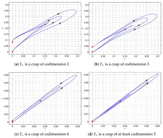
Figure 1. (a) When $q=2$, $m={\displaystyle \frac{3}{5}}$, $s={\displaystyle \frac{1}{2}}$, $h={\displaystyle \frac{12943}{78800}}$, $n={\displaystyle \frac{3}{100}}$ and $k={\displaystyle \frac{1617}{19700}}$, $E_{*}$ is a cusp of codimension 2. (b) When $q={\displaystyle \frac{3}{10}}$, $m={\displaystyle \frac{7}{20}}$, $s={\displaystyle \frac{7}{30}}$, $h={\displaystyle \frac{99}{400}}$, $n={\displaystyle \frac{3}{40}}$, and $k={\displaystyle \frac{3}{70}}$, $E_{*}$ is a cusp of codimension 3. (c) When $q\approx 0.6782414404$, $m\approx 0.5200915684$, $s={\displaystyle \frac{1}{2}}$, $h\approx 0.3128535566$, $n\approx 0.001028793414$, and $k\approx 0.001531275454$, $E_{*}$ is a cusp of codimension 4. (d) When $q\approx 0.5012295808$, $m\approx 0.5084479544$, $s={\displaystyle \frac{1}{2}}$, $h\approx 0.2438096618$, $n\approx 0.0004325794618$, and $k\approx 0.0005946513878$, $E_{*}$ is a cusp of at least codimension 5.

When $m\ne m_3$ and $m=m_4$, we have $d_{20}\ne 0$ and $d_{11}=0$. According to Lemma 2.4 in [42], the system (15) becomes

$$\begin{array}{c}{\displaystyle \dot{x_3}=y_3,}\hfill \\ {\displaystyle \dot{y_3}=x_3^2+\overline{M}{x}_3^3{y}_3+\overline{N}{x}_3^4{y}_3+o\left({|x_3,y_3|}^5\right),}\hfill \end{array}$$

where

$$\overline{M}=-{\displaystyle \frac{s^5{f}_1}{x_{*}{(q+x_{*})}^2(2x_{*}^2+x_{*}q+x_{*}s+qs-x_{*}){(4x_{*}^2+2x_{*}q+x_{*}s+qs-2x_{*})}^3}},$$

$$\overline{N}={\displaystyle \frac{s^8{f}_2}{x_{*}^2{(q+x_{*})}^3{(2x_{*}^2+x_{*}q+x_{*}s+qs-x_{*})}^2{(4x_{*}^2+2x_{*}q+x_{*}s+qs-2x_{*})}^5}},$$

where

$$\begin{array}{c}{f}_1=96x_{*}^9+96x_{*}^{8}q+384x_{*}^{8}s+24x_{*}^7{q}^2+480x_{*}^{7}qs+396x_{*}^7{s}^2+184x_{*}^6{q}^{2}s+424x_{*}^{6}q{s}^2\hfill \\ +132x_{*}^6{s}^3+28x_{*}^5{q}^{3}s-20x_{*}^5{q}^2{s}^2+166x_{*}^{5}q{s}^3-2x_{*}^5{s}^4+4x_{*}^4{q}^{4}s-116x_{*}^4{q}^3{s}^2\hfill \\ +90x_{*}^4{q}^2{s}^3+46x_{*}^{4}q{s}^4-8x_{*}^4{s}^5-32x_{*}^3{q}^4{s}^2+128x_{*}^3{q}^3{s}^3+138x_{*}^3{q}^2{s}^4+10x_{*}^{3}q{s}^5\hfill \\ -x_{*}^3{s}^6-4x_{*}^2{q}^5{s}^2+92x_{*}^2{q}^4{s}^3+140x_{*}^2{q}^3{s}^4+48x_{*}^2{q}^2{s}^5+x_{*}^{2}q{s}^6+22x_{*}{q}^5{s}^3\hfill \\ +54x_{*}{q}^4{s}^4+37x_{*}{q}^3{s}^5+5x_{*}{q}^2{s}^6+2q^6{s}^3+6q^5{s}^4+7q^4{s}^5+3q^3{s}^6-96x_{*}^8\hfill \\ -48x_{*}^{7}q-384x_{*}^{7}s-304x_{*}^{6}qs-348x_{*}^6{s}^2-68x_{*}^5{q}^{2}s-242x_{*}^{5}q{s}^2-80x_{*}^5{s}^3-12x_{*}^4{q}^{3}s\hfill \\ +66x_{*}^4{q}^2{s}^2-112x_{*}^{4}q{s}^3+8x_{*}^4{s}^4+50x_{*}^3{q}^3{s}^2-122x_{*}^3{q}^2{s}^3-37x_{*}^{3}q{s}^4+3x_{*}^3{s}^5\hfill \\ +10x_{*}^2{q}^4{s}^2-138x_{*}^2{q}^3{s}^3-99x_{*}^2{q}^2{s}^4-5x_{*}^{2}q{s}^5-50x_{*}{q}^4{s}^3-71x_{*}{q}^3{s}^4-16x_{*}{q}^2{s}^5\hfill \\ -6q^5{s}^3-13q^4{s}^4-8q^3{s}^5+24x_{*}^7+120x_{*}^{6}s+52x_{*}^{5}qs+94x_{*}^5{s}^2+12x_{*}^4{q}^{2}s+58x_{*}^{4}q{s}^2\hfill \\ +8x_{*}^4{s}^3-4x_{*}^3{q}^2{s}^2+41x_{*}^{3}q{s}^3-3x_{*}^3{s}^4-6x_{*}^2{q}^3{s}^2+53x_{*}^2{q}^2{s}^3+9x_{*}^{2}q{s}^4+34x_{*}{q}^3{s}^3\hfill \\ +17x_{*}{q}^2{s}^4+6q^4{s}^3+7q^3{s}^4-12x_{*}^{5}s-4x_{*}^{4}qs-8x_{*}^4{s}^2-14x_{*}^{3}q{s}^2+x_{*}^3{s}^3-2x_{*}^2{q}^2{s}^2\hfill \\ -7x_{*}^{2}q{s}^3-6x_{*}{q}^2{s}^3-2q^3{s}^3+2x_{*}^{2}q{s}^2,\hfill \end{array}$$

and the expression of $f_2$ is omitted for simplicity.

According to $(m,q,x_{*},s)\in \mathsf{\Omega }$ and $y_{*}=x_{*}+k_{*}$, we obtain

$$y_{*}=-{\displaystyle \frac{x_{*}m(2x_{*}^2+x_{*}q+s{x}_{*}+qs-x_{*})}{s(m{x}_{*}-s{x}_{*}-qs)}},$$

note that $m_4>0$ and $y_{*}>0$, which implies that $4x_{*}^2+2x_{*}q+x_{*}s+qs-2x_{*}\ne 0$ and $2x_{*}^2+x_{*}q+s{x}_{*}+qs-x_{*}\ne 0$. Therefore, whether $\overline{M}$ and $\overline{N}$ are equal to 0 is determined by $f_1$ and $f_2$, respectively.

According to Lemma 2.4 in [42], when $m=m_4$, $E_{*}$ is a cusp of codimension 3 if $f_1\ne 0$ (see Figure 1b), a cusp of codimension 4 if $f_1=0$, $f_2\ne 0$, or a cusp of codimension at least 5 if $f_1=0$, $f_2=0$. □

Because the conditions of Theorem 1 are very complex, the following remark gives two examples to show that the existence of the cusp of codimension 4 and at least 5.

Studying cusps with a codimension of at least 5 helps to more accurately predict the future development trends of ecosystems. By analyzing the system behavior near the cusp, we can identify under what circumstances the ecosystem may undergo abrupt changes, such as an increased risk of extinction for predator or prey populations. This is of great significance for early warning of the dynamic risks of ecosystems. Meanwhile, researching such cusps can help us uncover the complex dynamic behaviors of predator–prey systems with the interaction of multiple parameters, such as sudden changes in population sizes and alterations in system stability.

When the equilibrium point of the system is cusp-type, it depicts a sudden and irreversible drastic transformation of the population state in the ecosystem with minor changes in key parameters. The research results can be used to warn of the critical risk of the ecosystem and optimize ecological restoration strategies.

Remark 1.

(1) When $q\approx 0.6782414404$, $m\approx 0.5200915684$, $s={\displaystyle \frac{1}{2}}$, $h\approx 0.3128535566$, $n\approx 0.001028793414$, and $k\approx 0.001531275454$, $E_{*}$ is a cusp of codimension 4 (see Figure 1c).

(2) When $q\approx 0.5012295808$, $m\approx 0.5084479544$, $s={\displaystyle \frac{1}{2}}$, $h\approx 0.2438096618$, $n\approx 0.0004325794618$, and $k\approx 0.0005946513878$, $E_{*}$ is a cusp of codimension 5 (see Figure 1d).

Proof. 

Substituting $s={\displaystyle \frac{1}{2}}$ into $f_1$ and $f_2$, we obtain

$$\begin{array}{c}{f}_1=96x_{*}^{8}q+24x_{*}^7{q}^2+192x_{*}^{7}q+92x_{*}^6{q}^2+14x_{*}^5{q}^3+2x_{*}^4{q}^4-46x_{*}^{6}q-39x_{*}^5{q}^2-35x_{*}^4{q}^3\hfill \\ -8x_{*}^3{q}^4-x_{*}^2{q}^5-{\displaystyle \frac{55}{4}}{x}_{*}^{5}q+{\displaystyle \frac{135}{4}}{x}_{*}^4{q}^2+{\displaystyle \frac{57}{2}}{x}_{*}^3{q}^3+14x_{*}^2{q}^4+{\displaystyle \frac{11}{4}}{x}_{*}{q}^5+{\displaystyle \frac{11}{8}}{x}_{*}^{4}q-{\displaystyle \frac{61}{8}}{x}_{*}^3{q}^2\hfill \\ -10x_{*}^2{q}^3-{\displaystyle \frac{23}{8}}{x}_{*}{q}^4-{\displaystyle \frac{3}{8}}{x}_{*}^{3}q+{\displaystyle \frac{23}{16}}{x}_{*}^2{q}^2+{\displaystyle \frac{31}{32}}{x}_{*}{q}^3+{\displaystyle \frac{3}{64}}{x}_{*}^{2}q-{\displaystyle \frac{7}{64}}{x}_{*}{q}^2+96x_{*}^9+96x_{*}^8\hfill \\ -69x_{*}^7-{\displaystyle \frac{21}{2}}{x}_{*}^6+{\displaystyle \frac{1}{4}}{q}^6+{\displaystyle \frac{59}{8}}{x}_{*}^5-{\displaystyle \frac{3}{8}}{q}^5-{\displaystyle \frac{3}{4}}{x}_{*}^4+{\displaystyle \frac{5}{32}}{q}^4+{\displaystyle \frac{1}{64}}{x}_{*}^3-{\displaystyle \frac{1}{64}}{q}^3,\hfill \end{array}$$

and the expression of $f_2$ is given in Appendix A.

Computation with Maple yields the following resultant

$$\begin{array}{c}\mathrm{res}(f_1,f_2,q)=-{\displaystyle \frac{9x_{*}^{21}\left(48x_{*}^2+32x_{*}-5\right)\left(96x_{*}^4+208x_{*}^3+116x_{*}^2-16x_{*}+1\right){\left(4x_{*}^2+6x_{*}-1\right)}^3{\left(x_{*}-1\right)}^8{\left(8x_{*}^2+8x_{*}-1\right)}^{20}{g}_1}{75557863725914323419136}},\hfill \end{array}$$

where

$$\begin{array}{c}{g}_1=521838526464x_{*}^{20}+6729542664192x_{*}^{19}+29965852606464x_{*}^{18}+68080977838080x_{*}^{17}\hfill \\ +88935480950784x_{*}^{16}+65008176201728x_{*}^{15}+18813971595264x_{*}^{14}-6688124600320x_{*}^{13}\hfill \\ -6070966534144x_{*}^{12}-495059662848x_{*}^{11}+585921032192x_{*}^{10}+74417978624x_{*}^9\hfill \\ -27388345088x_{*}^8-986444992x_{*}^7+410979040x_{*}^6-5557496x_{*}^5+645360x_{*}^4-363533x_{*}^3\hfill \\ +24277x_{*}^2-552x_{*}+4.\hfill \end{array}$$

Next, the root isolation algorithm for multivariate polynomial systems [42,44] is applied to find a root of $f_1$ in $\mathsf{\Omega }$ and a common root of $f_1$ and $f_2$ in $\mathsf{\Omega }$, respectively. Let $f^{+}(x,y)$ denote the sum of the positive terms in $f(x,y)$ and $f^{-}(x,y)$ denote the sum of the negative terms in $f(x,y)$ [44].

Using “realroot$(g_1,{\displaystyle \frac{1}{{10}^{30}}})$” in Maple, $g_1\left(x_{*}\right)$ has four real roots in $x_{*}\in \mathsf{\Omega }$, where we only consider the second root as follows

$$\begin{array}{c}{x}_{*2}\in [{\underline{x}}_{*2},{\overline{x}}_{*2}],\hfill \end{array}$$

where

$$\begin{array}{c}{\underline{x}}_{*2}={\displaystyle \frac{292330194765549465342566325589729106869070581}{11417981541647679048466287755595961091061972992}},\hfill \\ \\ {\overline{x}}_{*2}={\displaystyle \frac{146165097382774732671283162794864553434535331}{5708990770823839524233143877797980545530986496}}.\hfill \end{array}$$

For $[{\underline{x}}_{*2},{\overline{x}}_{*2}]$ of $g_1\left(x_{*}\right)$, we obtain four positive real roots isolation intervals of $\{g_1\left(x_{*}\right),f_1(x_{*},q)\}$ in $\mathsf{\Omega }$. For brevity, we only consider the third and fourth roots as follows

$$\begin{array}{c}{q}_3\in [{\underline{q}}_3,{\overline{q}}_3],q_4\in [{\underline{q}}_4,{\overline{q}}_4],\hfill \end{array}$$

where

$$\begin{array}{c}{\underline{q}}_3={\displaystyle \frac{5860382824675954844838246562870260500501964693271}{11692013098647223345629478661730264157247460343808}},\hfill \\ \\ {\overline{q}}_3={\displaystyle \frac{2930191412337977422419123281435130250250984941349}{5846006549323611672814739330865132078623730171904}};\hfill \\ \\ {\underline{q}}_4={\displaystyle \frac{121002316357540282464105336352156349020927205}{178405961588244985132285746181186892047843328}},\hfill \\ \\ {\overline{q}}_4={\displaystyle \frac{242004632715080564928210672704312698041854653}{356811923176489970264571492362373784095686656}},\hfill \end{array}$$

by direct calculation, we have $f_2(x_{*2},q_3)<f_2^{-}({\underline{x}}_{*2},{\underline{q}}_3)+f_2^{+}({\overline{x}}_{*2},{\overline{q}}_3)\approx 3.043410947\times {10}^{-45}$, $f_2(x_{*2},q_3)>f_2^{-}({\overline{x}}_{*2},{\overline{q}}_3)+f_2^{+}({\underline{x}}_{*2},{\underline{q}}_3)\approx -3.043405037\times {10}^{-45}$, and $f_2(x_{*2},q_4)<f_2^{-}({\underline{x}}_{*2},{\underline{q}}_4)+f_2^{+}({\overline{x}}_{*2},{\overline{q}}_3)\approx -0.00004745918613$. Hence, $(x_{*2},q_3)$ is the common root of $f_1$ and $f_2$. $(x_{*2},q_4)$ is the root of $f_1$ but not the root of $f_2$.

Therefore, when $q\approx 0.6782414404$, $m\approx 0.5200915684$, $s={\displaystyle \frac{1}{2}}$, $h\approx 0.3128535566$, $n\approx 0.001028793414$, and $k\approx 0.001531275454$, that is, $f_1=0,f_2\ne 0$, $E_{*}$ is a cusp of codimension 4. When $q\approx 0.5012295808$, $m\approx 0.5084479544$, $s={\displaystyle \frac{1}{2}}$, $h\approx 0.2438096618$, $n\approx 0.0004325794618$, and $k\approx 0.0005946513878$, that is, $f_1=f_2=0$, $E_{*}$ is a cusp of codimension at least 5. □

3.2. A Triple Positive Equilibrium

For convenience, let the triple positive equilibrium $E_{123}$ be denoted by $E_{*}(x_{*},y_{*})$, where $y_{*}=x_{*}+k$. From the analysis in Section 3.1 and by simple computation, when $(h,n,k,m)=(h_{*},n_{*},k_{*},m_3)$ and $(m_3,q,x_{*},s)\in \mathsf{\Omega }$, which implies that $F\left(x_{*}\right)=F^{\prime }\left(x_{*}\right)=F^{″}\left(x_{*}\right)=Tr{J}_{E_{*}}=0$ and $F^{‴}\left(x_{*}\right)=6\ne 0$, it is obvious that $E_{*}(x_{*},y_{*})$ is a triple positive equilibrium.

Define

$$\begin{array}{c}{f}_3=16x_{*}^4+8x_{*}^{3}q+25x_{*}^{3}s+23x_{*}^{2}qs+6x_{*}^2{s}^2+7x_{*}{q}^{2}s+8x_{*}q{s}^2+x_{*}{s}^3+q^{3}s+2q^2{s}^2\hfill \\ +q{s}^3-8x_{*}^3-14x_{*}^{2}s-8x_{*}qs-2x_{*}{s}^2-2s{q}^2-2q{s}^2+x_{*}s+sq,\hfill \\ G_0=60x_{*}^6+60x_{*}^{5}q+120x_{*}^{5}s+15x_{*}^4{q}^2+130x_{*}^{4}qs+64x_{*}^4{s}^2+23x_{*}^3{q}^{2}s+85x_{*}^{3}q{s}^2\hfill \\ +14x_{*}^3{s}^3-10x_{*}^2{q}^{3}s+17x_{*}^2{q}^2{s}^2+23x_{*}^{2}q{s}^3+2x_{*}^2{s}^4-2x_{*}{q}^{4}s-9x_{*}{q}^3{s}^2+9x_{*}{q}^2{s}^3\hfill \\ +4x_{*}q{s}^4-2q^4{s}^2+2q^2{s}^4-60x_{*}^5-30x_{*}^{4}q-106x_{*}^{4}s-48x_{*}^{3}qs-39x_{*}^3{s}^2+19x_{*}^2{q}^{2}s\hfill \\ -27x_{*}^{2}q{s}^2-5x_{*}^2{s}^3+6x_{*}{q}^{3}s+10x_{*}{q}^2{s}^2-5x_{*}q{s}^3+4q^3{s}^2+15x_{*}^4+25x_{*}^{3}s-8x_{*}^{2}qs\hfill \\ +4x_{*}^2{s}^2-6x_{*}{q}^{2}s-x_{*}q{s}^2-2q^2{s}^2-x_{*}^{2}s+2x_{*}qs.\hfill \end{array}$$

Next, according to the method in [42], our goal is to determine the type of the triple positive equilibrium $E_{*}(x_{*},y_{*})$.

Theorem 2.

When $(h,n,k,m)=(h_{*},n_{*},k_{*},m_3)$, $(m_3,q,x_{*},s)\in \mathsf{\Omega }$, and $G_0\ne 0$, the triple positive equilibrium $E_{*}(x_{*},y_{*})$ is

(1)

A nilpotent focus of codimension 3 if $f_3<0$;

(2)

A nilpotent elliptic equilibrium of codimension 3 if $f_3>0$;

(3)

A nilpotent elliptic equilibrium of codimension at least 4 if $f_3=0$.

Proof. 

When $(h,n,k,m)=(h_{*},n_{*},k_{*},m_3)$ and $(m_3,q,x_{*},s)\in \mathsf{\Omega }$, using the transformations (11) and (13) in the proof of Theorem 1, system (6) becomes

$$\begin{array}{c}{\displaystyle {\dot{x}}_3=y_3+\sum _{3\le i+j\le 5}{c}_{ij}{x}_3^i{y}_3^j+o\left({|x_3,y_3|}^5\right),}\hfill \\ {\displaystyle {\dot{y}}_3=d_{20}{x}_3^2+d_{11}{x}_3{y}_3+\sum _{3\le i+j\le 5}{d}_{ij}{x}_2^i{y}_2^j+o\left({|x_3,y_3|}^5\right),}\hfill \end{array}$$

(15)

where

$$\begin{array}{c}{\displaystyle d_{20}=0,d_{11}=-\frac{s^2{n}_{*}}{x_{*}^2{m}_3},d_{30}=-\frac{s^4}{m_3(q+x_{*})},}\hfill \\ {\displaystyle 3c_{30}(d_{11}^2+5d_{30})+5d_{21}{d}_{30}-3d_{11}{d}_{40}=-\frac{s^6(x_{*}+q)G_0}{x_{*}{y}_{*}{h}_{*}{m}_3^2},}\hfill \\ {\displaystyle d_{11}^2+8d_{30}=\frac{s^5{f}_3}{x_{*}^2{(x_{*}+s)}^2{m}_3^2(q+x_{*})}.}\hfill \end{array}$$

When $(h,n,k,m)=(h_{*},n_{*},k_{*},m_3)$, $(m_3,q,x_{*},s)\in \mathsf{\Omega }$ and $G_0\ne 0$, it is easy to see that $d_{11}<0,d_{30}<0$ and $3c_{30}(d_{11}^2+5d_{30})+5d_{21}{d}_{30}-3d_{11}{d}_{40}\ne 0$. Obviously, the sign of $d_{11}^2+8d_{30}$ is determined by $f_3$. According to Lemma $2.5$ in [42], we obtain

(1) If $f_3<0$, $E_{*}$ is a nilpotent focus of codimension 3 (see Figure 2a);

(2) If $f_3>0$, $E_{*}$ is a nilpotent elliptic equilibrium of codimension 3 (see Figure 2b);

(3) If $f_3=0$, $E_{*}$ is a nilpotent elliptic equilibrium of codimension at least 4 (see Figure 2c).

□

Figure 2. (a) When $q={\displaystyle \frac{1}{4}}$, $m={\displaystyle \frac{11}{26}}$, $s={\displaystyle \frac{1}{3}}$, $h={\displaystyle \frac{4459}{23200}}$, $n={\displaystyle \frac{7}{260}}$, and $k={\displaystyle \frac{61}{11600}}$, $E_{*}$ is a nilpotent focus of codimension 3. (b) When $q={\displaystyle \frac{1}{5}}$, $m={\displaystyle \frac{14}{23}}$, $s={\displaystyle \frac{1}{3}}$, $h={\displaystyle \frac{115}{1168}}$, $n={\displaystyle \frac{19}{460}}$, and $k={\displaystyle \frac{61}{1825}}$, $E_{*}$ is a nilpotent elliptic equilibrium of codimension 3. (c) When $q={\displaystyle \frac{1}{5}}$, $m={\displaystyle \frac{8}{15}}$, $s={\displaystyle \frac{4}{15}}$, $h={\displaystyle \frac{32}{225}}$, $n={\displaystyle \frac{1}{15}}$, and $k={\displaystyle \frac{1}{30}}$, $E_{*}$ is a nilpotent elliptic equilibrium of codimension at least 4.

Figure 2. (a) When $q={\displaystyle \frac{1}{4}}$, $m={\displaystyle \frac{11}{26}}$, $s={\displaystyle \frac{1}{3}}$, $h={\displaystyle \frac{4459}{23200}}$, $n={\displaystyle \frac{7}{260}}$, and $k={\displaystyle \frac{61}{11600}}$, $E_{*}$ is a nilpotent focus of codimension 3. (b) When $q={\displaystyle \frac{1}{5}}$, $m={\displaystyle \frac{14}{23}}$, $s={\displaystyle \frac{1}{3}}$, $h={\displaystyle \frac{115}{1168}}$, $n={\displaystyle \frac{19}{460}}$, and $k={\displaystyle \frac{61}{1825}}$, $E_{*}$ is a nilpotent elliptic equilibrium of codimension 3. (c) When $q={\displaystyle \frac{1}{5}}$, $m={\displaystyle \frac{8}{15}}$, $s={\displaystyle \frac{4}{15}}$, $h={\displaystyle \frac{32}{225}}$, $n={\displaystyle \frac{1}{15}}$, and $k={\displaystyle \frac{1}{30}}$, $E_{*}$ is a nilpotent elliptic equilibrium of codimension at least 4.

4. Bifurcation

The study of high-codimension bifurcations in predator–prey systems not only reveals the underlying laws of ecosystems with the interaction of multiple factors but also provides quantitative support for solving “practical multi-objective and multi-constraint ecological management problems” and thus holds considerable practical significance for ecosystem conservation. Hence, this section analyzes the codimension-3 cusp-type degenerate Bogdanov–Takens bifurcation and the Hopf bifurcation in system (6).

4.1. Degenerate Bogdanov–Takens Bifurcation of Codimension 3

Theorem 1 (2) implies that the double positive equilibrium $E_{*}$ is a cusp of codimension 3. Consequently, a codimension-3 cusp-type degenerate Bogdanov–Takens bifurcation occurs near $E_{*}$. By selecting three parameters, the ecological mechanism of the system (6) can be quantified as the critical point of the dynamic system, and the vulnerability of the ecosystem under multiple pressures can be revealed through nonlinear dynamics. Hence, choosing m, n, and h as the bifurcation parameters, system (6) becomes

$$\begin{array}{c}{\displaystyle \dot{x}=x(1-x)-\frac{(m+{\lambda }_1)xy}{n_{*}+{\lambda }_2+x}-\frac{(h_{*}+{\lambda }_3)x}{q+x},}\hfill \\ {\displaystyle \dot{y}=sy\left(1-\frac{y}{x+k_{*}}\right).}\hfill \end{array}$$

(16)

where $\lambda =({\lambda }_1,{\lambda }_2,{\lambda }_3)$ is a parameter vector in a small neighborhood of the origin. Now, by a series of near-identity transformations, we will transform system (16) into the following universal unfolding:

$$\begin{array}{c}{\displaystyle \dot{x}=y,}\hfill \\ {\displaystyle \dot{y}={\mu }_1+{\mu }_{2}y+{\mu }_{3}xy+x^2\pm x^{3}y+\mathsf{\Phi }(x,y,\mu ),}\hfill \end{array}$$

(17)

where

$$\mathsf{\Phi }(x,y,\mu )=y^{2}o\left({|x,y|}^2\right)+o\left({|x,y|}^5\right)+o\left(\left|\mu \right|\right)o\left({\left|y\right|}^2\right)+o\left({|x,y|}^3\right)+o\left({\left|\mu \right|}^2\right)o\left(|x,y|\right),$$

and check ${\left|{\displaystyle \frac{\partial ({\mu }_1,{\mu }_2,{\mu }_3)}{\partial ({\lambda }_1,{\lambda }_2,{\lambda }_3)}}\right|}_{\lambda =0}$≠ 0.

Define

$$\begin{array}{c}\widehat{f}=24x_{*}^4+24x_{*}^{3}q+18x_{*}^{3}s+4x_{*}^2{q}^2+7x_{*}^{2}qs+3x_{*}^2{s}^2-12x_{*}{q}^{2}s-3s{q}^3-3q^2{s}^2\hfill \\ -12x_{*}^3-6x_{*}^{2}q-5x_{*}^{2}s+3q^{2}s+2x_{*}^2.\hfill \end{array}$$

Theorem 3.

System (6) undergoes a cusp-type degenerate Bogdanov–Takens bifurcation of codimension 3 around $E_{*}$ if $\widehat{f}\ne 0$ and the condition of Theorem 1 (2) holds.

Proof. 

Firstly, using the following transformation

$$x=X+x_{*},y=Y+x_{*}+k,$$

system (16) takes the form

$$\begin{array}{c}{\displaystyle \dot{X}=a_{00}+a_{10}X+a_{01}Y+a_{20}{X}^2+a_{11}XY+a_{30}{X}^3+a_{21}{X}^{2}Y}\hfill \\ +a_{40}{X}^4+a_{31}{X}^{3}Y+o\left({|X,Y|}^4\right),\hfill \\ {\displaystyle \dot{Y}=b_{00}+b_{10}X+b_{01}Y+b_{20}{X}^2+b_{11}XY+b_{02}{Y}^2+b_{30}{X}^3+B_{21}{X}^{2}Y}\hfill \\ +b_{12}X{Y}^2+b_{40}{X}^4+b_{31}{X}^{3}Y+b_{22}{X}^2{Y}^2+o\left({|X,Y|}^4\right),\hfill \end{array}$$

(18)

with the coefficients omitted. In the following proof, the coefficients are also omitted.

Secondly, letting $x=X$ and $y=\dot{X}$, system (18) becomes

$$\begin{array}{c}{\displaystyle \dot{x}=y,}\hfill \\ {\displaystyle \dot{y}=c_{00}+c_{10}x+c_{01}y+c_{20}{x}^2+c_{11}xy+c_{02}{y}^2+c_{30}{x}^3+c_{21}{x}^{2}y}\hfill \\ +c_{12}x{y}^2+c_{40}{x}^4+c_{31}{x}^{3}y+c_{22}{x}^2{y}^2+o\left({|x,y|}^4\right).\hfill \end{array}$$

(19)

Next, inspired by [26], we transform system (19) into system (17) through the following six steps.

(1) Eliminating the $y^2$-term in system (19), we let $x=X+{\displaystyle \frac{c_{02}}{2}}{X}^2$ and $y=Y+c_{02}XY$, and system (19) transforms into

$$\begin{array}{c}{\displaystyle \dot{X}=Y,}\hfill \\ {\displaystyle \dot{Y}=d_{00}+d_{10}X+d_{01}Y+d_{20}{X}^2+d_{11}XY+d_{30}{X}^3+d_{21}{X}^{2}Y}\hfill \\ +d_{12}X{Y}^2+d_{40}{X}^4+d_{31}{X}^{3}Y+d_{22}{X}^2{Y}^2+o\left({|X,Y|}^4\right).\hfill \end{array}$$

(20)

(2) To eliminate the $X{Y}^2$-term in system (20), we let $X=x+{\displaystyle \frac{d_{12}}{6}}{x}^3$ and $Y=y+{\displaystyle \frac{d_{12}}{2}}{x}^{2}y$, and system (20) becomes

$$\begin{array}{c}{\displaystyle \dot{x}=y,}\hfill \\ {\displaystyle \dot{y}=e_{00}+e_{10}x+e_{01}y+e_{20}{x}^2+e_{11}xy+e_{30}{x}^3+e_{21}{x}^{2}y}\hfill \\ +e_{40}{x}^4+e_{31}{x}^{3}y+e_{22}{x}^2{y}^2+o\left({|x,y|}^4\right).\hfill \end{array}$$

(21)

(3) When $\lambda =0$, it is easy to see that $e_{20}{|}_{\lambda =0}=-{\displaystyle \frac{s^3{n}_{*}}{2m_4{x}_{*}^2}}\ne 0$. To eliminate the $x^3$-term and $x^4$-term in system (21), let

$$\begin{array}{c}x=X-{\displaystyle \frac{e_{30}}{4e_{20}}}{X}^2+{\displaystyle \frac{15e_{30}^2-16e_{20}{e}_{40}}{80e_{20}^2}}{X}^3,y=Y,t=(1-{\displaystyle \frac{e_{30}}{2e_{20}}}X+{\displaystyle \frac{45e_{30}^2-48e_{20}{e}_{40}}{80e_{20}^2}}{X}^2)\tau ,\hfill \end{array}$$

then system (21) becomes

$$\begin{array}{c}{\displaystyle \dot{X}=Y,}\hfill \\ {\displaystyle \dot{Y}=f_{00}+f_{10}X+f_{01}Y+f_{20}{X}^2+f_{11}XY+f_{30}{X}^3+f_{21}{X}^{2}Y}\hfill \\ +f_{40}{X}^4+f_{31}{X}^{3}Y+p_1(X,Y,\lambda ),\hfill \end{array}$$

(22)

where $p_1(X,Y,\lambda )$ has the property of $\mathsf{\Phi }(x,y,\mu )$ and $f_{30}=f_{40}=0$ if $\lambda =0$.

(4) Clearly $f_{20}{|}_{\lambda =0}=-{\displaystyle \frac{s^3{n}_{*}}{2m_4{x}_{*}^2}}\ne 0$. To eliminate the $X^{2}Y$-term in system (22), we let

$$\begin{array}{c}X=x,Y=y+{\displaystyle \frac{f_{21}}{3f_{20}}}{y}^2+{\displaystyle \frac{f_{21}^2}{36f_{20}^2}}{y}^3,t=(1+{\displaystyle \frac{f_{21}}{3f_{20}}}y+{\displaystyle \frac{f_{21}^2}{36f_{20}^2}}{y}^2)\tau ,\hfill \end{array}$$

then system (22) becomes

$$\begin{array}{c}{\displaystyle \dot{x}=y,}\hfill \\ {\displaystyle \dot{y}=g_{00}+g_{10}x+g_{01}y+g_{20}{x}^2+g_{11}xy+g_{31}{x}^{3}y+p_2(x,y,\lambda ),}\hfill \end{array}$$

(23)

where $p_2(X,Y,\lambda )$ has the property of $\mathsf{\Phi }(x,y,\mu )$.

(5) From system (23), $n_{*}>0,m_4>0$ and $y_{*}>0$, we have

$$\begin{array}{c}{g}_{20}{|}_{\lambda =0}=-{\displaystyle \frac{s^3{n}_{*}}{2m_4{x}_{*}^2}}\ne 0,\hfill \\ g_{31}{|}_{\lambda =0}={\displaystyle \frac{f_1}{\left(3x_{*}+q+s-1\right)s{\left(4x_{*}^2+2x_{*}q+s{x}_{*}+qs-2x_{*}\right)}^2\left(2x_{*}^2+x_{*}q+s{x}_{*}+qs-x_{*}\right){\left(q+x_{*}\right)}^2{x}_{*}}}\ne 0.\hfill \end{array}$$

Reducing the coefficients of $x_2$ and $x^{3}y$ to 1 and $-1$ in system (23), respectively, let

$$\begin{array}{c}x=g_{20}^{{\displaystyle \frac{1}{5}}}{g}_{31}^{-{\displaystyle \frac{2}{5}}}X,y=-g_{20}^{{\displaystyle \frac{4}{5}}}{g}_{31}^{-{\displaystyle \frac{3}{5}}}Y,t=-g_{20}^{-{\displaystyle \frac{3}{5}}}{g}_{31}^{{\displaystyle \frac{1}{5}}}\tau ,\hfill \end{array}$$

then system (23) becomes

$$\begin{array}{c}{\displaystyle \dot{X}=Y,}\hfill \\ {\displaystyle \dot{Y}=h_{00}+h_{10}X+h_{01}Y+X^2+h_{11}XY-X^{3}Y+p_3(X,Y,\lambda ),}\hfill \end{array}$$

(24)

where $p_3(X,Y,\lambda )$ has the property of $\mathsf{\Phi }(x,y,\mu )$.

(6) To eliminate the X-term in system (24), let $x=X+{\displaystyle \frac{h_{10}}{2}}$ and $y=Y$, then system (24) becomes

$$\begin{array}{c}{\displaystyle \dot{x}=y,}\hfill \\ {\displaystyle \dot{y}={\mu }_1+{\mu }_{2}y+x^2+{\mu }_{3}xy-x^{3}y+p_4(X,Y,\lambda ),}\hfill \end{array}$$

(25)

where $p_4(x,y,\lambda )$ has the property of $\mathsf{\Phi }(x,y,\mu )$.

Note that $\widehat{f}\ne 0,m_4>0,n_{*}>0,h_{*}>0$. Finally, by Maple software 2024.2, we obtain that

$$\begin{array}{c}{\left|{\displaystyle \frac{\partial ({\mu }_1,{\mu }_2,{\mu }_3)}{\partial ({\lambda }_1,{\lambda }_2,{\lambda }_3)}}\right|}_{\lambda =0}\hfill \\ ={\displaystyle \frac{{(2x_{*}^2+x_{*}s-qs)}^{\frac{16}{5}}\widehat{f}{f}_1^{\frac{4}{5}}}{x_{*}^{\frac{9}{5}}{s}^{\frac{28}{5}}{(4x_{*}^2+2x_{*}q+s{x}_{*}+qs-2x_{*})}^{\frac{6}{5}}{(3x_{*}+s+q-1)}^{\frac{21}{5}}{(q+x_{*})}^{\frac{23}{5}}(6x_{*}^3+4x_{*}^{2}q+2x_{*}^{2}s+x_{*}qs-q^{2}s-2x_{*}^2)}}\ne 0.\hfill \end{array}$$

Since system (25) is the versal unfolding of the codimension-3 Bogdanov–Takens singularity [45], it follows that system (16) undergoes a codimension-3 cusp-type degenerate Bogdanov–Takens bifurcation. The proof is completed. □

4.2. Hopf Bifurcation

According to Lemma 3, we know that $Det{J}_{E_i}>0$$(i=1,3)$. System (6) may undergo Hopf bifurcation around $E_i$ if $Tr{J}_{E_i}=0$$(i=1,3)$. For the sake of simplicity, we denote $E_i(x_i,x_i+k)$$(i=1,3)$ by $E_z(z,z+k)$. Next, we prove that Hopf bifurcation will occur around $E_z$.

From $F\left(z\right)=Tr{J}_{E_z}=0$, we have

$$\begin{array}{c}{\displaystyle h=\overline{h}=\frac{{\left(q+z\right)}^2((n+z)s-z(1-n-2z))}{\left(n-q\right)z},}\hfill \\ {\displaystyle m=\overline{m}=\frac{{\left(n+z\right)}^2(z(1-q-2z)-(q+z)s)}{z\left(n-q\right)\left(z+k\right)}.}\hfill \end{array}$$

The Jacobian matrix of system (6) at $E_z$ is

$$J_{E_z}=\left(\begin{array}{cc}s& {\displaystyle -\frac{(n+z)\left(z\right(1-q-2z)-(q+z\left)s\right)}{(n-q)(z+k)}}\\ s& -s\end{array}\right),$$

which implies that $Det{J}_{E_z}$ is

$${\displaystyle Det{J}_{E_z}=\frac{s^2}{z+k}\left(\frac{(n+z)\left(z\right(1-q-2z)-(q+z\left)s\right)-zs(n-q)}{s\left(n-q\right)}-k\right).}$$

Define

$$\begin{array}{c}{\displaystyle {\widehat{s}}_1=\frac{z\left(1-n-2z\right)}{n+z},{\widehat{s}}_2=\frac{z\left(1-q-2z\right)}{q+z},}\hfill \\ {\displaystyle {\widehat{k}}_1=\frac{(n+z)\left(z\right(1-q-2z)-(q+z\left)s\right)-zs(n-q)}{s\left(n-q\right)},}\hfill \\ \mathsf{\Pi }:={\mathsf{\Pi }}_1\cup {\mathsf{\Pi }}_2,\hfill \end{array}$$

where

$$\begin{array}{c}{\mathsf{\Pi }}_1:=\{(n,q,s,k,z)\mid 0<q<n,\max \{{\widehat{s}}_1,0\}<s<{\widehat{s}}_2,0<k<{\widehat{k}}_1\},\hfill \\ {\mathsf{\Pi }}_2:=\{(n,q,s,k,z)\mid 0<n<q,\max \{{\widehat{s}}_2,0\}<s<{\widehat{s}}_1,0<k<{\widehat{k}}_1\}.\hfill \end{array}$$

To ensure that $\overline{m}>0$, $\overline{h}>0$ and $Det{J}_{E_z}>0$, we obtain $(n,q,s,k,z)\in \mathsf{\Pi }$.

Next, our objective is to compute the focal values of the equilibrium point $E_z$. First, using:

$$\begin{array}{c}x=x_1+z,y=y_1+z+k;\hfill \\ {\displaystyle x_1=-\frac{a_{10}{a}_{01}}{a_{10}^2+d}{x}_2-\frac{a_{01}\sqrt{d}}{a_{10}^2+d}{y}_2,y_1=x_2,\tau =\sqrt{d}t,}\hfill \end{array}$$

where

$$\begin{array}{c}{\displaystyle a_{10}=s,a_{01}=-\frac{\left(n+z\right)(z(1-q-2z)-(q+z)s)}{\left(n-q\right)\left(z+k\right)},b_{10}=s,b_{01}=-s,}\hfill \\ d=a_{10}{b}_{01}-a_{01}{b}_{10}=Det{J}_{E_z},\hfill \end{array}$$

system (6) becomes

$$\begin{array}{c}{\dot{x}}_2=y_2+c_{02}{y}_2^2+c_{12}{x}_2{y}_2^2+c_{03}{y}_2^3+o\left({|x_2,y_2|}^3\right),\hfill \\ {\dot{y}}_2=-x_2+d_{20}{x}_2^2+d_{11}{x}_2{y}_2+d_{02}{y}_2^2+d_{30}{x}_2^3+d_{21}{x}_2^2{y}_2\hfill \\ +d_{12}{x}_2{y}_2^2+d_{03}{y}_2^3+o\left({|x_2,y_2|}^3\right),\hfill \end{array}$$

where the coefficients are omitted for brevity.

From [41] and by Maple, we obtain the first two Lyapunov coefficients as follows:

$$\begin{array}{c}{\displaystyle L_1=\frac{(z(1-q-2z)-(q+z)s)l_1}{4z{\left(n-q\right)}^2{\left(z+k\right)}^3\left(n+z\right){\left(q+z\right)}^2{d}^{\frac{3}{2}}},}\hfill \\ {\displaystyle L_2=\frac{(z(1-q-2z)-(q+z)s)l_2}{24z^3{\left(n-q\right)}^4{\left(z+k\right)}^7{\left(n+z\right)}^3{\left(q+z\right)}^4{d}^{\frac{5}{2}}},}\hfill \end{array}$$

where the expression of $l_1$ is given in Appendix A and the expression of $l_2$ is omitted for simplicity. When $(n,q,s,k,z)\in \mathsf{\Pi }$, we obtain that all variables in $L_i(i=1,2)$ are non-zero except for $l_i(i=1,2)$. Then, we have the following theorem.

Theorem 4.

Assume that $m=\overline{m}$, $h=\overline{h}$ and $(n,q,s,k,z)\in \mathsf{\Pi }$.

(1) If $L_1<0$, $E_z$ is a stable weak focus with a multiplicity of one, and system (6) undergoes a supercritical Hopf bifurcation;

(2) If $L_1>0$, $E_z$ is an unstable weak focus with a multiplicity of one, and system (6) undergoes a subcritical Hopf bifurcation;

(3) If $L_1=0$, $E_z$ is a weak focus with a multiplicity of at least two, and system (6) undergoes a degenerate Hopf bifurcation.

Given the highly complex expressions for the focal values of system (6), its exact codimension is analytically intractable. Consequently, numerical calculations indicate that this system possesses a weak focus of multiplicity two or higher.

Firstly, we give an example to show that $E_z$ is a weak focus with a multiplicity of two, that is, $L_1=0$ and $L_2\ne 0$. When $q={\displaystyle \frac{1}{5}}$, $n={\displaystyle \frac{1}{4}}$, $s={\displaystyle \frac{8}{45}}$, $k={\displaystyle \frac{-10529+81\sqrt{115105}}{113890}}$, $h={\displaystyle \frac{4}{25}}$, and $m={\displaystyle \frac{-1361+9\sqrt{115105}}{3280}}$, by calculation, we can obtain $L_1=0$ and $L_2\approx 82.24634710>0$. Then $E_z({\displaystyle \frac{1}{5}},{\displaystyle \frac{12249+81\sqrt{115105}}{113890}})$ is an unstable weak focus with a multiplicity of two.

Next, we show that $E_z$ is a weak focus with a multiplicity of at least three, that is, $L_1=L_2=0$. When $q=0.2$, $n=0.4$, $s\approx 0.10398454$, $k\approx 0.49178075$, $h\approx 0.08956291$, and $m\approx 0.49966068$, by calculation, we can obtain $L_1=L_2=0$. Then $E_z(0.2,0.69178075)$ is a weak focus with a multiplicity of at least three.

From ref. [39], for system (3) with constant-yield harvesting, that is, system (5), the authors showed that the system has a weak focus with a multiplicity of at most two. However, with the influence of Michaelis–Menten-type harvesting, we show that system (6) has a weak focus with a multiplicity of at least three. Therefore, compared with the system (5), the Michaelis–Menten-type harvesting leads to more complex dynamics for the system (6).

5. Numerical Simulations

This section provides numerical simulations to corroborate our central results, specifically the codimension-3 cusp-type degenerate Bogdanov–Takens bifurcation established for system (6) in Theorem 3. Letting

$$(n,s,k,h)=\left({\displaystyle \frac{1}{4}},{\displaystyle \frac{8}{45}},{\displaystyle \frac{-10529+81\sqrt{115105}}{113890}},{\displaystyle \frac{4}{25}}\right),$$

Figure 3 presents the two-parameter bifurcation diagram constructed with the Matcont 7.1 software.

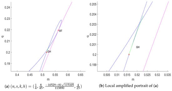
Figure 3. Bifurcation diagram of cusp-type degenerate Bogdanov–Takens bifurcation for system (6) in the $(m,q)$ plane with $(n,s,k,h)=({\displaystyle \frac{1}{4}},{\displaystyle \frac{8}{45}},{\displaystyle \frac{-10529+81\sqrt{115105}}{113890}},{\displaystyle \frac{4}{25}})$. The solid blue, green, and magenta lines depict the Hopf bifurcation, degenerate Hopf bifurcation, and saddle-node bifurcation, respectively.

Based on Figure 3, we plotted the phase portraits of system (6) for different values of parameter q, with the parameter $m=0.518$. The detailed dynamic behaviors corresponding to these phase portraits are summarized in Table 1. As shown in Table 1, with the increase in parameter q, system (6) successively undergoes a sequence of bifurcations: saddle-node bifurcation, saddle-node bifurcation of limit cycle, supercritical Hopf bifurcation, and homoclinic bifurcation. Hence, with the influence of Michaelis–Menten-type prey harvesting, some complex phenomena occur in system (6).

Table 1. Dynamical behaviors of system (6) in Figure 3 with $(n,s,k,h)=({\displaystyle \frac{1}{4}},{\displaystyle \frac{8}{45}},{\displaystyle \frac{-10529+81\sqrt{115105}}{113890}},{\displaystyle \frac{4}{25}})$ (The phase portraits are shown in Figure 4).

q	${\mathit{E}}_2$	${\mathit{E}}_3$	Limit Cycle and Homoclinic Loop
0.15	No	No	No (Figure 4a)
0.2	Saddle	Unstable focus	No (Figure 4b)
0.201197	Saddle	Unstable focus	An stable limit cycle (inner)
			An unstable limit cycle (outer) (see Figure 4c)
0.201218	Saddle	Stable focus	An unstable limit cycle (see Figure 4d)
0.201229	Saddle	Stable focus	A homoclinic loop (Figure 4e)
0.202	Saddle	Stable focus	No (Figure 4f)
0.24	No	Stable focus	No (Figure 4g)

Figure 4. Phase portraits are shown for system (6) for the parameter values $(n,s,k,h)=({\displaystyle \frac{1}{4}},{\displaystyle \frac{8}{45}},{\displaystyle \frac{-10529+81\sqrt{115105}}{113890}},{\displaystyle \frac{4}{25}})$. The detailed dynamic behavior is described in Table 1. The red curve in (c) represents the stable limit cycle, while the green curves in (c,d) represent the unstable limit cycle.

Figure 4. Phase portraits are shown for system (6) for the parameter values $(n,s,k,h)=({\displaystyle \frac{1}{4}},{\displaystyle \frac{8}{45}},{\displaystyle \frac{-10529+81\sqrt{115105}}{113890}},{\displaystyle \frac{4}{25}})$. The detailed dynamic behavior is described in Table 1. The red curve in (c) represents the stable limit cycle, while the green curves in (c,d) represent the unstable limit cycle.

6. Conclusions

This study presents a comprehensive analysis of a Holling–Tanner predator–prey model with a generalist predator and Michaelis–Menten-type prey harvesting. Our findings indicate that system (6) can possess up to three positive equilibria and four boundary equilibria, with the latter potentially being saddle-nodes, degenerate stable nodes, or degenerate saddles.

Considering system (6) with constant-yield harvesting, which is referred to as system (4), the authors of [39] demonstrated that this system possesses a cusp of codimension 4 and a weak focus of order 2. They further established that it undergoes a codimension-2 degenerate Hopf bifurcation, giving rise to two limit cycles. Gupta and Chandra [46] studied the stability and bifurcation of the system when $b=k_1$ in system (5). However, they did not obtain the codimension of the cusp and Bogdanov–Takens bifurcation. Moreover, both the systems in [39,46] have at most two positive equilibria. Compared with [39,46], system (6) has at most three positive equilibria. It is proven that the double positive equilibrium is a cusp with a codimension of at least 5 and that system (6) has a weak focus with a multiplicity of at least 3. This indicates that, due to the influence of nonlinear harvesting, we obtain the cusp and weak focus with higher codimensions than those in [39,46]. From Theorem 2, the triple positive equilibrium is a nilpotent focus (or elliptic) of codimension 3 or a nilpotent elliptic equilibrium of codimension at least 4, which is not presented in [39,46]. Additionally, we prove that system (6) undergoes several bifurcations, including a codimension-3 cusp-type degenerate Bogdanov–Takens bifurcation and a Hopf bifurcation. Finally, we employed numerical simulations to confirm our main theoretical results and demonstrate the existence of two limit cycles in the system. In the research on system (6), we find the Michaelis–Menten-type harvesting leads to more complex dynamics. Based on the research on this system presented in this paper, we know that in reality, when predators prey on prey species, there exists a critical conservation threshold. When the population size falls below this threshold, predation must be suspended to prevent extinction. We can use this to predict the dynamic risks of the ecosystem, intervene in advance, and formulate flexible multi-objective management strategies.

Appendix A.1. The Expression of l₁

$$\begin{array}{c}{l}_1=k^2{n}^{3}q{s}^2+k^2{n}^{3}qsz+2k^2{n}^{3}s{z}^2+2k^2{n}^3{z}^3+3k^2{n}^{2}q{s}^{2}z+6k^2{n}^{2}qs{z}^2+2k^2{n}^{2}q{z}^3\hfill \\ +10k^2{n}^{2}s{z}^3+12k^2{n}^2{z}^4-k^{2}n{q}^3{s}^2-k^{2}n{q}^{3}sz-3k^{2}n{q}^2{s}^{2}z-8k^{2}n{q}^{2}s{z}^2-2k^{2}n{q}^2{z}^3\hfill \\ -6k^{2}nqs{z}^3-k^{2}n{s}^2{z}^3+6k^{2}ns{z}^4+18k^{2}n{z}^5-2k^2{q}^3{z}^3-4k^2{q}^{2}s{z}^3-12k^2{q}^2{z}^4\hfill \\ +k^{2}q{s}^2{z}^3-6k^{2}qs{z}^4-18k^{2}q{z}^5+k{n}^3{q}^2{s}^2+4k{n}^3{q}^{2}sz+2k{n}^3{q}^2{z}^2+3k{n}^{3}q{s}^{2}z\hfill \\ +8k{n}^{3}qs{z}^2+3k{n}^{3}q{z}^3+3k{n}^{3}s{z}^3+2k{n}^3{z}^4+2k{n}^2{q}^3{s}^2+3k{n}^2{q}^{3}sz+2k{n}^2{q}^3{z}^2\hfill \\ +6k{n}^2{q}^2{s}^{2}z+20k{n}^2{q}^{2}s{z}^2+14k{n}^2{q}^2{z}^3+9k{n}^{2}q{s}^2{z}^2+34k{n}^{2}qs{z}^3+20k{n}^{2}q{z}^4\hfill \\ -k{n}^2{s}^2{z}^3+16k{n}^{2}s{z}^4+16k{n}^2{z}^5-kn{q}^{3}s{z}^2+2kn{q}^3{z}^3-3kn{q}^2{s}^2{z}^2-8kn{q}^{2}s{z}^3\hfill \\ +8kn{q}^2{z}^4-3knq{s}^2{z}^3-11knqs{z}^4+7knq{z}^5-6kn{s}^2{z}^4-3kns{z}^5+18kn{z}^6\hfill \\ -2k{q}^{3}s{z}^3-4k{q}^3{z}^4-2k{q}^2{s}^2{z}^3-16k{q}^{2}s{z}^4-24k{q}^2{z}^5-3kq{s}^2{z}^4-27kqs{z}^5\hfill \\ -42kq{z}^6-3k{s}^2{z}^5-12ks{z}^6-12k{z}^7-n^3{q}^3{s}^2-n^3{q}^{3}sz+4n^3{q}^{2}s{z}^2+4n^3{q}^2{z}^3\hfill \\ +3n^{3}q{s}^2{z}^2+12n^{3}qs{z}^3+9n^{3}q{z}^4+n^3{s}^2{z}^3+5n^{3}s{z}^4+4n^3{z}^5+3n^2{q}^{3}s{z}^2+4n^2{q}^3{z}^3\hfill \\ +6n^2{q}^2{s}^2{z}^2+32n^2{q}^{2}s{z}^3+30n^2{q}^2{z}^4+12n^{2}q{s}^2{z}^3+58n^{2}qs{z}^4+52n^{2}q{z}^5+3n^2{s}^2{z}^4\hfill \\ +24n^{2}s{z}^5+24n^2{z}^6+3n{q}^{3}s{z}^3+6n{q}^3{z}^4+3n{q}^2{s}^2{z}^3+24n{q}^{2}s{z}^4+36n{q}^2{z}^5+6nq{s}^2{z}^4\hfill \\ +40nqs{z}^5+57nq{z}^6+15ns{z}^6+28n{z}^7-qs{z}^6-2q{z}^7-s^2{z}^6-2s{z}^7-k^2{n}^{2}qsz-2k^2{n}^{2}s{z}^2\hfill \\ -4k^2{n}^2{z}^3+k^{2}n{q}^{2}sz+2k^{2}nqs{z}^2-k^{2}ns{z}^3-12k^{2}n{z}^4+4k^2{q}^2{z}^3+k^{2}qs{z}^3+12k^{2}q{z}^4\hfill \\ -2k{n}^{3}qsz-2k{n}^{3}q{z}^2+k{n}^{3}s{z}^2+k{n}^3{z}^3-3k{n}^2{q}^{2}sz-4k{n}^2{q}^2{z}^2-11k{n}^{2}qs{z}^2\hfill \\ -13k{n}^{2}q{z}^3-k{n}^{2}s{z}^3-2k{n}^2{z}^4+kn{q}^{2}s{z}^2-4kn{q}^2{z}^3+2knqs{z}^3-8knq{z}^4+6kns{z}^4\hfill \\ -7kn{z}^5+2k{q}^{2}s{z}^3+8k{q}^2{z}^4+7kqs{z}^4+27kq{z}^5+6ks{z}^5+12k{z}^6+n^3{q}^{2}sz-2n^{3}qs{z}^2\hfill \\ -4n^{3}q{z}^3-n^3{z}^4-3n^2{q}^{2}s{z}^2-8n^2{q}^2{z}^3-16n^{2}qs{z}^3-31n^{2}q{z}^4-5n^{2}s{z}^4-12n^2{z}^5-3n{q}^{2}s{z}^3\hfill \\ -12n{q}^2{z}^4-12nqs{z}^4-38nq{z}^5-2ns{z}^5-17n{z}^6+q{z}^6+2s{z}^6+2z^7+2k^{2}n{z}^3-2k^{2}q{z}^3\hfill \\ +2k{n}^{2}q{z}^2-k{n}^2{z}^3+2knq{z}^3-4kq{z}^4-3k{z}^5+4n^{2}q{z}^3+n^2{z}^4+6nq{z}^4+2n{z}^5-z^6.\hfill \end{array}$$

Appendix A.2. The Expression of f₂

$$\begin{array}{c}{f}_2={\displaystyle \frac{1}{64}}{x}_{*}^2{q}^5-{\displaystyle \frac{19}{1024}}{x}_{*}^2{q}^4-{\displaystyle \frac{3}{512}}{q}^6-{\displaystyle \frac{5}{1024}}{x}_{*}^6-{\displaystyle \frac{4315}{32}}{x}_{*}^6{q}^3-{\displaystyle \frac{415}{512}}{x}_{*}^3{q}^4+{\displaystyle \frac{3605}{64}}{x}_{*}^7{q}^2+{\displaystyle \frac{361}{32}}{x}_{*}^{8}q-{\displaystyle \frac{1215}{4}}{x}_{*}^{11}\hfill \\ -{\displaystyle \frac{1}{16}}{q}^{10}+{\displaystyle \frac{1}{8}}{q}^9-{\displaystyle \frac{13}{128}}{q}^8+{\displaystyle \frac{5}{128}}{q}^7-{\displaystyle \frac{2263}{8}}{x}_{*}^{9}q+{\displaystyle \frac{27}{256}}{x}_{*}^3{q}^3+{\displaystyle \frac{245}{128}}{x}_{*}^{7}q+33856x_{*}^{13}{q}^2-2384x_{*}^{13}q\hfill \\ +480x_{*}^{12}{q}^4+17696x_{*}^{12}{q}^3+14004x_{*}^{12}{q}^2-23176x_{*}^{12}q+{\displaystyle \frac{121}{256}}{x}_{*}^7-{\displaystyle \frac{121}{256}}{x}_{*}^2{q}^6+3840x_{*}^{13}{q}^3\hfill \\ +15360x_{*}^{15}q+11520x_{*}^{14}{q}^2+28800x_{*}^{14}q+4294x_{*}^{12}-5400x_{*}^{13}-6768x_{*}^{14}-{\displaystyle \frac{1425}{128}}{x}_{*}^8+7680x_{*}^{15}\hfill \\ +7680x_{*}^{16}+{\displaystyle \frac{1663}{16}}{x}_{*}^9-{\displaystyle \frac{5715}{16}}{x}_{*}^{10}+{\displaystyle \frac{9}{1024}}{x}_{*}{q}^5+{\displaystyle \frac{35}{512}}{x}_{*}{q}^6+246x_{*}^8{q}^6+20x_{*}^7{q}^7+2x_{*}^6{q}^8-28588x_{*}^{11}{q}^2\hfill \\ -20833x_{*}^{10}{q}^3-12559x_{*}^9{q}^4-5337x_{*}^8{q}^5-1400x_{*}^7{q}^6-245x_{*}^6{q}^7-21x_{*}^5{q}^8-x_{*}^4{q}^9+8411x_{*}^{11}q\hfill \\ +{\displaystyle \frac{18127}{2}}{x}_{*}^{10}{q}^2+10336x_{*}^9{q}^3+{\displaystyle \frac{15359}{2}}{x}_{*}^8{q}^4+{\displaystyle \frac{7809}{2}}{x}_{*}^7{q}^5+{\displaystyle \frac{3109}{2}}{x}_{*}^6{q}^6+{\displaystyle \frac{811}{2}}{x}_{*}^5{q}^7+{\displaystyle \frac{289}{4}}{x}_{*}^4{q}^8+{\displaystyle \frac{13}{2}}{x}_{*}^3{q}^9\hfill \\ +{\displaystyle \frac{1}{4}}{x}_{*}^2{q}^{10}+{\displaystyle \frac{977}{8}}{x}_{*}^{10}q-{\displaystyle \frac{13865}{8}}{x}_{*}^9{q}^2-{\displaystyle \frac{23881}{8}}{x}_{*}^8{q}^3-{\displaystyle \frac{22331}{8}}{x}_{*}^7{q}^4-1868x_{*}^6{q}^5-{\displaystyle \frac{5521}{8}}{x}_{*}^5{q}^6-{\displaystyle \frac{335}{2}}{x}_{*}^4{q}^7\hfill \\ -{\displaystyle \frac{87}{4}}{x}_{*}^3{q}^8-{\displaystyle \frac{9}{4}}{x}_{*}^2{q}^9-{\displaystyle \frac{1}{8}}{x}_{*}{q}^{10}+{\displaystyle \frac{5527}{32}}{x}_{*}^8{q}^2+{\displaystyle \frac{8829}{16}}{x}_{*}^7{q}^3+{\displaystyle \frac{28601}{32}}{x}_{*}^6{q}^4+{\displaystyle \frac{7795}{16}}{x}_{*}^5{q}^5+{\displaystyle \frac{2325}{16}}{x}_{*}^4{q}^6+{\displaystyle \frac{111}{8}}{x}_{*}^3{q}^7\hfill \\ -{\displaystyle \frac{5}{16}}{x}_{*}^2{q}^8-{\displaystyle \frac{9}{16}}{x}_{*}{q}^9-{\displaystyle \frac{5393}{32}}{x}_{*}^5{q}^4-{\displaystyle \frac{2359}{32}}{x}_{*}^4{q}^5-{\displaystyle \frac{415}{64}}{x}_{*}^3{q}^6+{\displaystyle \frac{55}{32}}{x}_{*}^2{q}^7+{\displaystyle \frac{17}{16}}{x}_{*}{q}^8+{\displaystyle \frac{437}{128}}{x}_{*}^3{q}^5-{\displaystyle \frac{35}{64}}{x}_{*}{q}^7\hfill \\ +4560x_{*}^{11}{q}^4+656x_{*}^{10}{q}^5+64x_{*}^9{q}^6+14520x_{*}^{11}{q}^3+5700x_{*}^{10}{q}^4+1336x_{*}^9{q}^5-{\displaystyle \frac{25}{512}}{x}_{*}^4{q}^2-{\displaystyle \frac{1157}{512}}{x}_{*}^4{q}^3\hfill \\ +{\displaystyle \frac{4931}{256}}{x}_{*}^4{q}^4-{\displaystyle \frac{5}{1024}}{x}_{*}^{5}q+{\displaystyle \frac{327}{256}}{x}_{*}^5{q}^2+{\displaystyle \frac{2929}{128}}{x}_{*}^5{q}^3-{\displaystyle \frac{19}{512}}{x}_{*}^{6}q-{\displaystyle \frac{929}{64}}{x}_{*}^6{q}^2.\hfill \end{array}$$

References

- Dey, S.; Ghorai, S.; Banerjee, M. Analytical detection of stationary and dynamic patterns in a prey–predator model with reproductive Allee effect in prey growth. J. Math. Biol. 2023, 87, 21. [Google Scholar] [CrossRef]
- Li, S.; Yuan, S.; Jin, Z.; Wang, H. Bifurcation analysis in a diffusive predator-prey model with spatial memory of prey, Allee effect and maturation delay of predator. J. Differ. Equ. 2023, 357, 32–63. [Google Scholar] [CrossRef]
- Liu, Y.; Zhang, Z.; Li, Z. The impact of Allee effect on a Leslie-Gower predator-prey model with hunting cooperation. Qual. Theory Dyn. Syst. 2024, 23, 88. [Google Scholar] [CrossRef]
- Yuan, M.; Wang, N. Stability and bifurcation analysis for a predator-prey model with crowley-martin functional response. J. Nonlinear Model. Anal. 2025, 7, 1–19. [Google Scholar]
- Leslie, P. Some further notes on the use of matrices in population mathematics. Biometrika 1948, 35, 213–245. [Google Scholar] [CrossRef]
- Korobeinikov, A. A Lyapunov function for Leslie-Gower predator-prey models. Appl. Math. Lett. 2001, 14, 697–700. [Google Scholar] [CrossRef]
- Yin, W.; Li, Z.; Chen, F.; He, M. Modeling Allee effect in the Lesile-Gower predator-prey system incorporating a prey refuge. Int. J. Bifurc. Chaos 2022, 32, 2250086. [Google Scholar] [CrossRef]
- Arancibia-Ibarra, C.; Flores, J.; Pettet, G.; van Heijster, P. A Holling-Tanner predator-prey model with strong Allee effect. Int. J. Bifurc. Chaos 2019, 29, 1930032. [Google Scholar] [CrossRef]
- Dai, Y.; Zhao, Y.; Sang, B. Four limit cycles in a predator-prey system of Leslie type with generalized Holling type III functional response. Nonlinear Anal. Real World Appl. 2019, 50, 218–239. [Google Scholar] [CrossRef]
- Yang, Y.; Xu, Y.; Rong, L.; Ruan, S. Bifurcations and global dynamics of a predator-prey mite model of Leslie type. Stud. Appl. Math. 2024, 152, 1251–1304. [Google Scholar] [CrossRef]
- He, M.; Li, Z. Global dynamics of a Leslie-Gower predator-prey model with square root response function. Appl. Math. Lett. 2023, 140, 108561. [Google Scholar] [CrossRef]
- Chen, X.; Yang, W. Complex dynamical behaviors of a Leslie-Gower predator-prey model with herd behavior. J. Nonlinear Model. Anal. 2024, 6, 1064–1082. [Google Scholar]
- Li, Y.; He, M.; Li, Z. Dynamics of a ratio-dependent Leslie-Gower predator-prey model with Allee effect and fear effect. Math. Comput. Simul. 2022, 201, 417–439. [Google Scholar] [CrossRef]
- Ding, W.; Huang, W. Global dynamics of a ratio-dependent Holling-Tanner predator-prey system. J. Math. Anal. Appl. 2018, 460, 458–475. [Google Scholar] [CrossRef]
- Zhang, M.; Li, Z.; Chen, F.; Chen, L. Bifurcation analysis of a Leslie-Gower predator-prey model with Allee effect on predator and simplified Holling type IV functional response. Qual. Theory Dyn. Syst. 2025, 24, 131. [Google Scholar] [CrossRef]
- May, R. Stability and Complexity in Model Ecosystems; Princeton University Press: Princeton, NJ, USA, 1973. [Google Scholar]
- Hsu, S.; Huang, T. Global stability for a class of predator-prey systems. SIAM J. Appl. Math. 1995, 55, 763–783. [Google Scholar] [CrossRef]
- Sáez, E.; González-Olivares, E. Dynamics of a predator-prey model. SIAM J. Appl. Math. 1999, 59, 1867–1878. [Google Scholar] [CrossRef]
- Hanski, I.; Hansson, L.; Henttonen, H. Specialist predators, generalist predators, and the microtine rodent cycle. J. Anim. Ecol. 1991, 60, 353–367. [Google Scholar] [CrossRef]
- Sen, D.; Ghorai, S.; Sharma, S.; Banerjee, M. Allee effect in prey’s growth reduces the dynamical complexity in prey-predator model with generalist predator. Appl. Math. Model. 2021, 91, 768–790. [Google Scholar] [CrossRef]
- Zhang, Y.; Huang, J.; Wang, H. Bifurcations driven by generalist and specialist predation: Mathematical interpretation of Fennoscandia phenomenon. J. Math. Biol. 2023, 86, 94. [Google Scholar] [CrossRef]
- Xiang, C.; Huang, J.; Ruan, S.; Xiao, D. Bifurcation analysis in a host-generalist parasitoid model with Holling II functional response. J. Differ. Equ. 2020, 268, 4618–4662. [Google Scholar] [CrossRef]
- Zhang, M.; Li, Z. Bifurcation analysis of a modified Leslie-Gower predator-prey system with fear effect on prey. Discret. Contin. Dyn. Syst.-B 2025, 30, 3730–3760. [Google Scholar] [CrossRef]
- Aziz-Alaoui, M.; Okiye, M. Boundedness and global stability for a predator-prey model with modified Leslie-Gower and Holling-type II schemes. Appl. Math. Lett. 2003, 16, 1069–1075. [Google Scholar] [CrossRef]
- Nindjin, A.; Aziz-Alaoui, M.; Cadivel, M. Analysis of a predator-prey model with modified Leslie-Gower and Holling-type II schemes with time delay. Nonlinear Anal. Real World Appl. 2006, 7, 1104–1118. [Google Scholar] [CrossRef]
- Xiang, C.; Huang, J.; Wang, H. Linking bifurcation analysis of Holling-Tanner model with generalist predator to a changing environment. Stud. Appl. Math. 2022, 149, 124–163. [Google Scholar] [CrossRef]
- Chen, M.; Takeuchi, Y.; Zhang, J. Dynamic complexity of a modified Leslie-Gower predator-prey system with fear effect. Commun. Nonlinear Sci. Numer. Simul. 2023, 119, 107109. [Google Scholar] [CrossRef]
- Maiti, A.; Pathak, S. A modified Holling-Tanner model in stochastic environment. Nonlinear Anal. Model. Control 2009, 14, 51–71. [Google Scholar] [CrossRef]
- Tiwari, B.; Raw, S. Dynamics of Leslie-Gower model with double Allee effect on prey and mutual interference among predators. Nonlinear Dyn. 2021, 103, 1229–1257. [Google Scholar] [CrossRef]
- Cai, Y.; Zhao, C.; Wang, W.; Wang, J. Dynamics of a Leslie-Gower predator-prey model with additive Allee effect. Appl. Math. Model. 2015, 39, 2092–2106. [Google Scholar] [CrossRef]
- Xiang, C.; Huang, J.; Wang, H. Bifurcations in Holling-Tanner model with generalist predator and prey refuge. J. Differ. Equ. 2023, 343, 495–529. [Google Scholar] [CrossRef]
- Xu, Y.; Yang, Y.; Meng, F.; Ruan, S. Degenerate codimension-2 cusp of limit cycles in a Holling-Tanner model with harvesting and anti-predator behavior. Nonlinear Anal. Real World Appl. 2024, 76, 103995. [Google Scholar] [CrossRef]
- Huangfu, C.; Li, Z.; Chen, F.; Chen, L.; He, M. Dynamics of a harvested Leslie-Gower predator-prey model with simplified Holling type IV functional response. Int. J. Bifurc. Chaos 2025, 25, 550023. [Google Scholar] [CrossRef]
- Ma, Y.; Yang, R. Bifurcation analysis in a modified Leslie-Gower with nonlocal competition and Beddington-DeAngelis functional response. J. Appl. Anal. Comput. 2025, 15, 2152–2184. [Google Scholar] [CrossRef]
- Huang, J.; Gong, Y.; Chen, J. Multiple bifurcations in a predator-prey system of Holling and Leslie type with constant-yield prey harvesting. Int. J. Bifurc. Chaos 2013, 23, 1350164. [Google Scholar] [CrossRef]
- Zhu, C.; Lan, L. Phase portraits, Hopf bifurcations and limit cycles of Leslie-Gower predator-prey systems with harvesting rates. Discret. Contin. Dyn. Syst.-B 2010, 14, 289–306. [Google Scholar]
- Gupta, R.; Banerjee, M.; Chandra, P. Bifurcation analysis and control of Leslie-Gower predator-prey model with Michaelis-Menten type prey-harvesting. Differ. Equ. Dyn. Syst. 2012, 20, 339–366. [Google Scholar] [CrossRef]
- Yao, Y.; Liu, L. Dynamics of a Leslie-Gower predator-prey system with hunting cooperation and prey harvesting. Discret. Contin. Dyn. Syst.-B 2022, 27, 4787–4815. [Google Scholar] [CrossRef]
- Wu, H.; Li, Z.; He, M. Bifurcation analysis of a Holling-Tanner model with generalist predator and constant-yield harvesting. Int. J. Bifurc. Chaos 2024, 34, 2450076. [Google Scholar] [CrossRef]
- He, M.; Li, Z. Bifurcation of a Leslie-Gower predator-prey model with nonlinear harvesting and a generalist predator. Axioms 2024, 13, 704. [Google Scholar] [CrossRef]
- Zhang, Z.; Ding, T.; Huang, W.; Dong, Z. Qualitative Theory of Differential Equations; Translations of Mathematical Monographs; American Mathematical Society: Providence, RI, USA, 1992. [Google Scholar]
- Lu, M.; Huang, J.; Wang, H. An organizing center of codimension four in a predator-prey model with generalist predator: From tristability and quadristability to transients in a nonlinear environmental change. SIAM J. Appl. Dyn. Syst. 2023, 22, 694–729. [Google Scholar] [CrossRef]
- Perko, L. Differential Equations and Dynamical Systems; Springer: New York, NY, USA, 1996. [Google Scholar]
- Lu, Z.; He, B.; Luo, Y.; Pan, L. An algorithm of real root isolation for polynomial systems with applications to the construction of limit cycles. Symb.-Numer. Comput. 2007, 232, 131–147. [Google Scholar]
- Dumortier, F.; Roussarie, R.; Sotomayor, J. Generic 3-parameter families of vector fields on the plane, unfolding a singularity with nilpotent linear part. The cusp case of codimension 3. Ergod. Theory Dyn. Syst. 1987, 7, 375–413. [Google Scholar] [CrossRef]
- Gupta, R.; Chandra, P. Bifurcation analysis of modified Leslie-Gower predator-prey model with Michaelis-Menten type prey-harvesting. J. Math. Anal. Appl. 2013, 398, 278–295. [Google Scholar] [CrossRef]
Disclaimer/Publisher’s Note: The statements, opinions and data contained in all publications are solely those of the individual author(s) and contributor(s) and not of MDPI and/or the editor(s). MDPI and/or the editor(s) disclaim responsibility for any injury to people or property resulting from any ideas, methods, instructions or products referred to in the content. |
© 2025 by the authors. Licensee MDPI, Basel, Switzerland. This article is an open access article distributed under the terms and conditions of the Creative Commons Attribution (CC BY) license (https://creativecommons.org/licenses/by/4.0/).