Unit-Power Half-Normal Distribution Including Quantile Regression with Applications to Medical Data

Abstract

In this paper, we present the unit-power half-normal distribution, derived from the power half-normal distribution, for data analysis in the open unit interval. The statistical properties of the unit-power half-normal model are described in detail. Simulation studies are carried out to evaluate the performance of the parameter estimators. Additionally, we implement the quantile regression for this model, which is applied to two real healthcare data sets. Our findings suggest that the unit power half-normal distribution provides a robust and flexible alternative for existing models for proportion data.

1. Introduction

To study and interpret real events, new statistical models must continuously be built. In recent times, models limited to the interval $(0,1)$ have generated a lot of interest. This type of models is mainly used to study proportion data, such as survival rate data and product failure, among others. Different areas, such as health, actuarial and financial sciences, require this type of distributions. So, recently, several distributions with positive support have been transformed to distributions with unit support, such as the cases of Jones [1] in the Kumaraswamy distribution, Gómez-Déniz et al. [2] in the log-Lindley distribution, Mazucheli et al. [3], in the Lindley distribution, Abd El-Monsef et al. [4], who proposed a new two-parameter omega unitary distribution, Altun et al. [5], who studied a distribution called enhanced second-order Lindley distribution modeling data on the interval (0,1), and, recently, Ahmad et al. [6], who studied the exponential pareto distribution.

One of the distributions that is mainly used for this type of data is the Beta distribution. Interest in this type of model has been increasing, and many researchers have transformed known distributions with positive support into distributions with unitary support, an example of which can be found in articles such as Grassia [7], based on the Gamma distribution, Ghitany et al. [8], based on the Inverse Gamma distribution, Mazucheli et al. [9], based on the Birnbaum-Saunders distribution, Modi et al. [10], based on Burr distribution III, Korkmaz and Chesneau [11], based on Burr distribution XII, Haq et al. [12], based on the modified Burr III distribution, and, more recently, Bakouch et al. [13], based on half-normal distribution.

The aim of this paper is to introduce a new distribution with a bounded domain on (0,1). This distribution is originated by modifying the representation of the power half-normal (PHN) distribution proposed by Gómez et al. [14]. One of the motivations of this work is to generate alternatives to well-known distributions used in the statistical analysis of certain type of data. This work is based on the PHN distribution whose probability density function f (pdf), cumulative distribution function F (cdf), and quantile function Q are:

$$\begin{array}{ccc}\hfill f_Y(y;\sigma ,\alpha )& =& {\displaystyle \frac{2\alpha }{\sigma }}\varphi \left({\displaystyle \frac{y}{\sigma }}\right){\left(2\Phi \left({\displaystyle \frac{y}{\sigma }}-1\right)\right)}^{\alpha -1},y>0,\hfill \end{array}$$

(1)

$$\begin{array}{ccc}\hfill F_Y(y;\sigma ,\alpha )& =& {\left(2\Phi \left({\displaystyle \frac{y}{\sigma }}\right)-1\right)}^{\alpha },y>0,\hfill \end{array}$$

(2)

$$\begin{array}{ccc}\hfill Q(p;\sigma ,\alpha )& =& \sigma {\Phi }^{-1}\left({\displaystyle \frac{1+p^{1/\alpha }}{2}}\right),0<p<1,\hfill \end{array}$$

(3)

where the parameters are $\sigma >0$ and $\alpha >0$. $\varphi (·)$ and $\Phi (·)$ denote the pdf and cdf of the standard normal distribution, respectively.

At present, this model continues to be studied. For example, Barrios et al. [15] performed an extension of the distribution using the slash process, resulting in a model with higher kurtosis, i.e., with heavier tails. In addition, Pallini [16] introduced a discretized model based on the PHN distribution. The interest in further investigating models with support on the interval (0,1) is of great importance, since in many areas, such as finance, actuarial sciences, engineering, and health, databases that belong to this type of interval are handled. To consider a new model with unit support based on the PHN model is a promising alternative for more accurate inferential studies.

The rest of the paper is organized as follows. In Section 2, we introduce our proposal, the unit-power half-normal (UPHN) distribution. Several important properties of this new model are presented. In Section 3, inference is performed, and maximum likelihood (ML) estimators are obtained. In Section 4, the reparametrized model in terms of a quantile is presented. In Section 5, a simulation study is carried out to analyse the performance of ML estimators in finite samples for the proposed model without and with covariates. In Section 6, two real data applications are presented, and we are again dealing with cases without and with covariates. Finally, in Section 7, some concluding comments are presented.

2. Unit Power Half-Normal Distribution

In this section, we will discuss the stochastic representation of the UPHN model, including its pdf, cdf, and some properties of the model.

2.1. Stochastic Representation

Definition 1.

A random variable X follows a $UPHN$ distribution with parameters $\sigma >0$ and $\alpha >0$ if its stochastic representation is given by:

$$X={\displaystyle \frac{1}{1+Y}}$$

(4)

where $Y\sim PHN(\sigma ,\alpha )$. The notation $X\sim UPHN(\sigma ,\alpha )$ will be used.

2.2. Pdf, Cdf, Survival, and Hazard Functions

Proposition 1.

Let $X\sim UPHN(\sigma ,\alpha )$. Then, the pdf of X is given by:

$$\begin{array}{ccc}\hfill f_X(x;\sigma ,\alpha )& =& {\displaystyle \frac{2\alpha }{\sigma x^2}}\varphi \left({\displaystyle \frac{1-x}{\sigma x}}\right){\left(2\Phi \left({\displaystyle \frac{1-x}{\sigma x}}\right)-1\right)}^{\alpha -1},0<x<1,\sigma ,\alpha >0.\hfill \end{array}$$

(5)

Proof. 

By considering the stochastic representation given in (4), $x=g\left(y\right)=1/(1+y)$, we have that

$$f_X(x;\sigma ,\alpha )=f_Y(g^{-1}\left(x\right);\sigma ,\alpha )\left|{\displaystyle \frac{d{g}^{-1}\left(x\right)}{dx}}\right|={\displaystyle \frac{2\alpha }{\sigma }}\varphi \left({\displaystyle \frac{g^{-1}\left(x\right)}{\sigma }}\right){\left(2\Phi \left({\displaystyle \frac{g^{-1}\left(x\right)}{\sigma }}\right)-1\right)}^{\alpha -1}{\displaystyle \frac{1}{x^2}}.$$

Taking into account that $g^{-1}\left(x\right)=(1-x)/x$, (5) follows.    □

Proposition 2.

Let $X\sim UPHN(\sigma ,\alpha )$. Then, its cdf is given by:

$$F(x;\sigma ,\alpha )=\left\{\begin{array}{cc}0,\hfill & x\le 0,\hfill \\ 1-{\left(2\Phi \left({\displaystyle \frac{1-x}{\sigma x}}\right)-1\right)}^{\alpha },\hfill & 0<x<1,\hfill \\ 1,\hfill & x\ge 1.\hfill \end{array}\right.$$

(6)

Proof. 

• If $x\le 0$, then $f\left(x\right)=0$. Therefore, $F(x,\sigma ,\alpha )=0$.
• It follows from the fact that for $0<x<1$,

  $$F(x;\sigma ,\alpha )={\int }_0^x{\displaystyle \frac{2\alpha }{\sigma t^2}}\varphi \left({\displaystyle \frac{1-t}{\sigma t}}\right){\left(2\Phi \left({\displaystyle \frac{1-t}{\sigma t}}\right)-1\right)}^{\alpha -1}dt.$$
  Making $u=2\Phi \left({\displaystyle \frac{1-t}{\sigma t}}\right)-1$, we obtain the result.
• If $x\ge 1$, then:

  $$\begin{array}{ccc}\hfill F(x;\sigma ,\alpha )& =& {\int }_{-\infty }^{x}f\left(t\right)dt\hfill \\ & =& {\int }_{-\infty }^{0}0dt+{\int }_0^1{\displaystyle \frac{2\alpha }{\sigma t^2}}\varphi \left({\displaystyle \frac{1-t}{\sigma t}}\right){\left(2\Phi \left({\displaystyle \frac{1-t}{\sigma t}}\right)-1\right)}^{\alpha -1}dt+{\int }_1^{x}0dt=1.\hfill \end{array}$$

   □

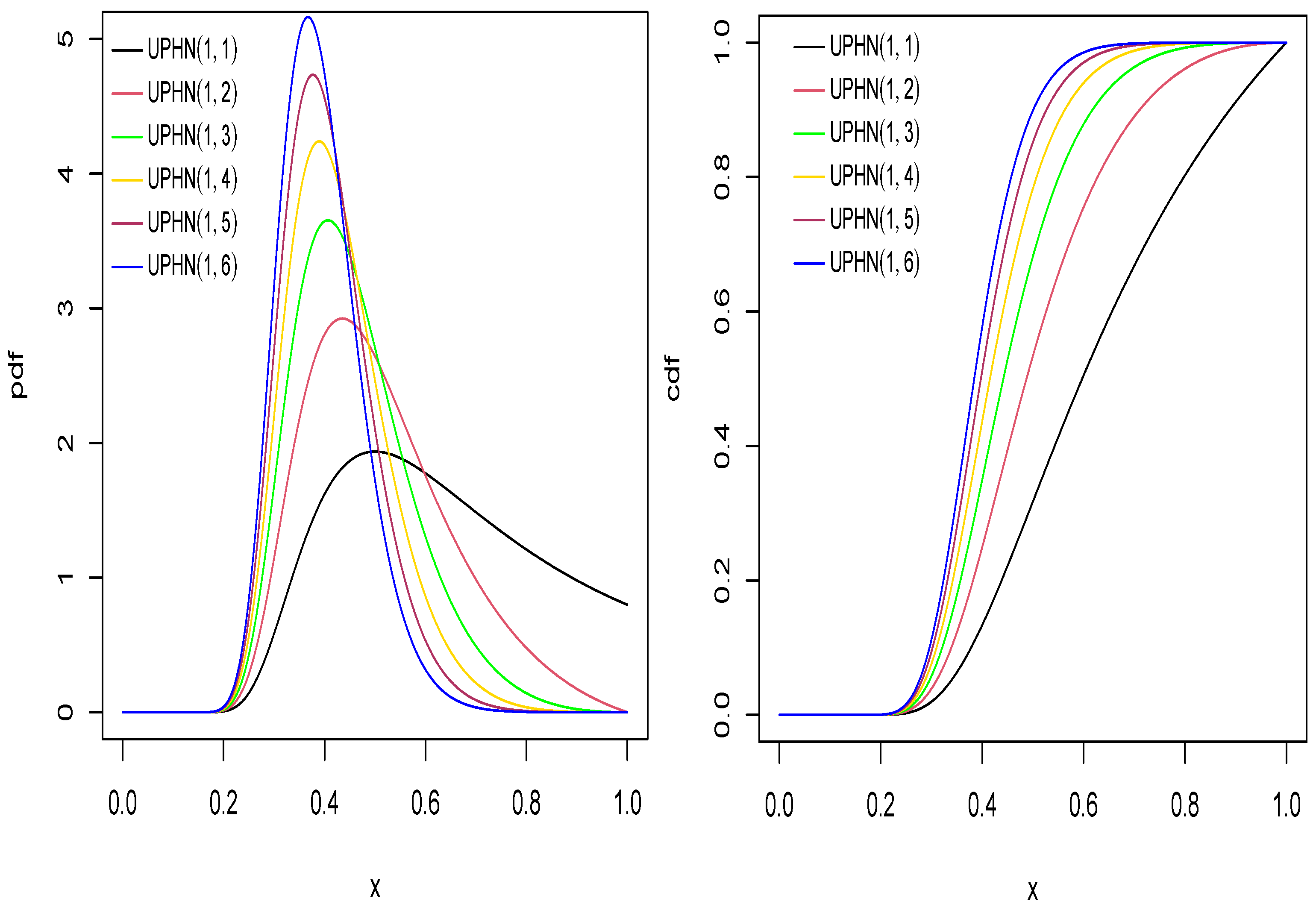
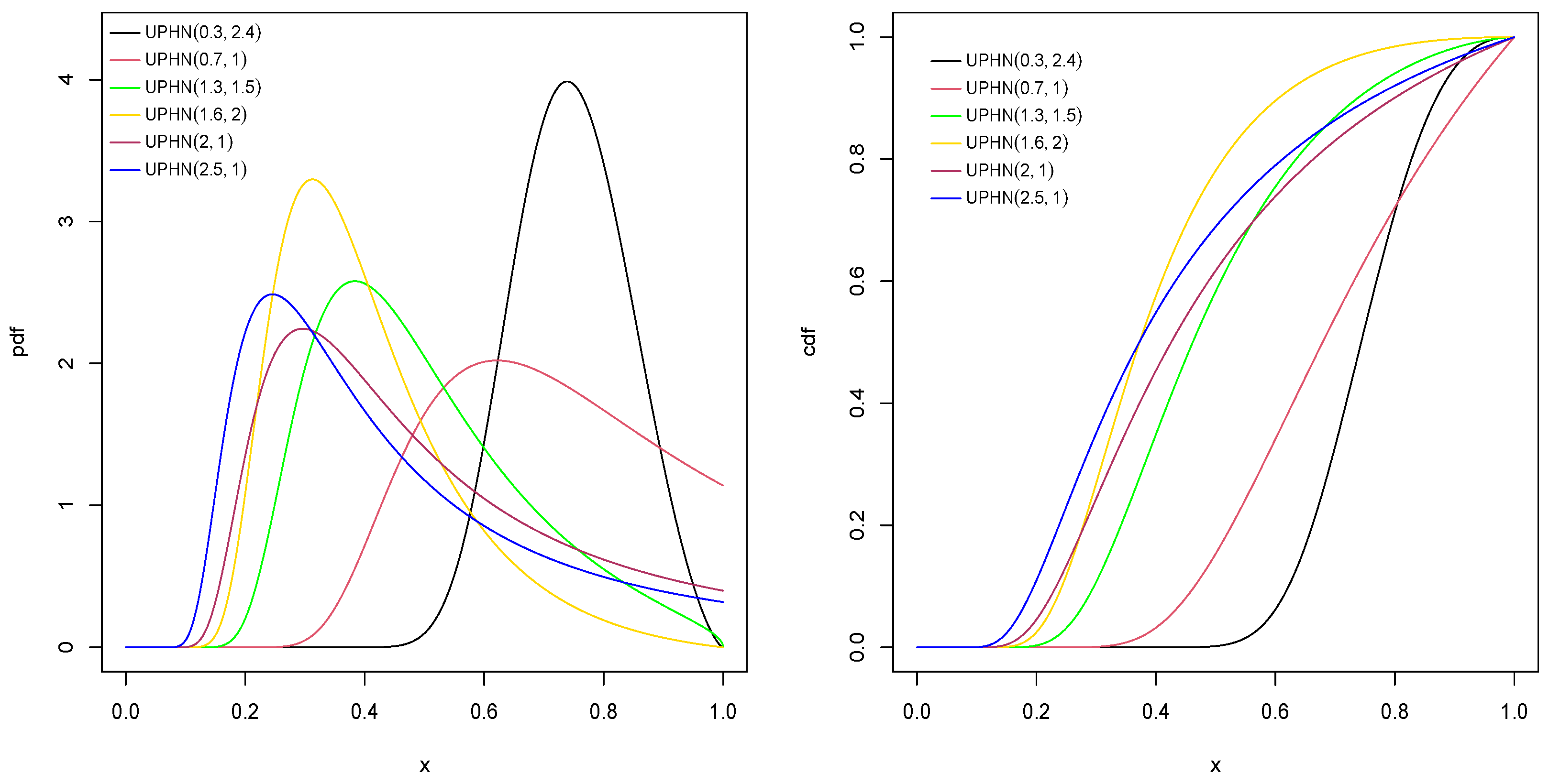
Figure 1 shows the pdf and cdf of the UPHN$(\sigma ,\alpha )$ model of $\sigma =1$ with different values for $\alpha$. Figure 2 shows the pdf and cdf of the UPHN$(\sigma ,\alpha )$ model, for different values of $(\sigma ,\alpha )$.

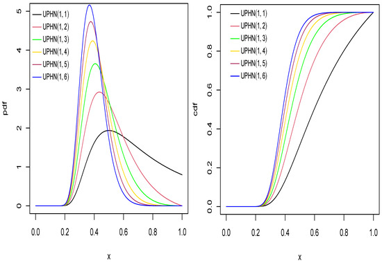
Figure 1. Pdf and cdf for UPHN$(\sigma =1,\alpha )$ model with different values of $\alpha$.

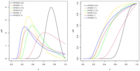
Figure 2. Pdf and cdf for UPHN$(\sigma ,\alpha )$ model for some values of parameters $\sigma$ and $\alpha$.

Proposition 3.

Let $X\sim UPHN(\sigma ,\alpha )$. Then, the survival and hazard function of X are given by:

$$\begin{array}{ccc}\hfill S(x;\sigma ,\alpha )={\left(2\Phi \left({\displaystyle \frac{1-x}{\sigma x}}\right)-1\right)}^{\alpha }andh(x;\sigma ,\alpha )& =& {\displaystyle \frac{2\alpha }{\sigma x^2}}\varphi \left({\displaystyle \frac{1-x}{\sigma x}}\right){\left(2\Phi \left({\displaystyle \frac{1-x}{\sigma x}}\right)-1\right)}^{-1},\hfill \end{array}$$

for $0<x<1$.

Proof. 

Both functions are immediately obtained from their definitions, since $S\left(x\right)=1-F\left(x\right)$ and $h\left(x\right)={\displaystyle \frac{f\left(x\right)}{1-F\left(x\right)}}$.    □

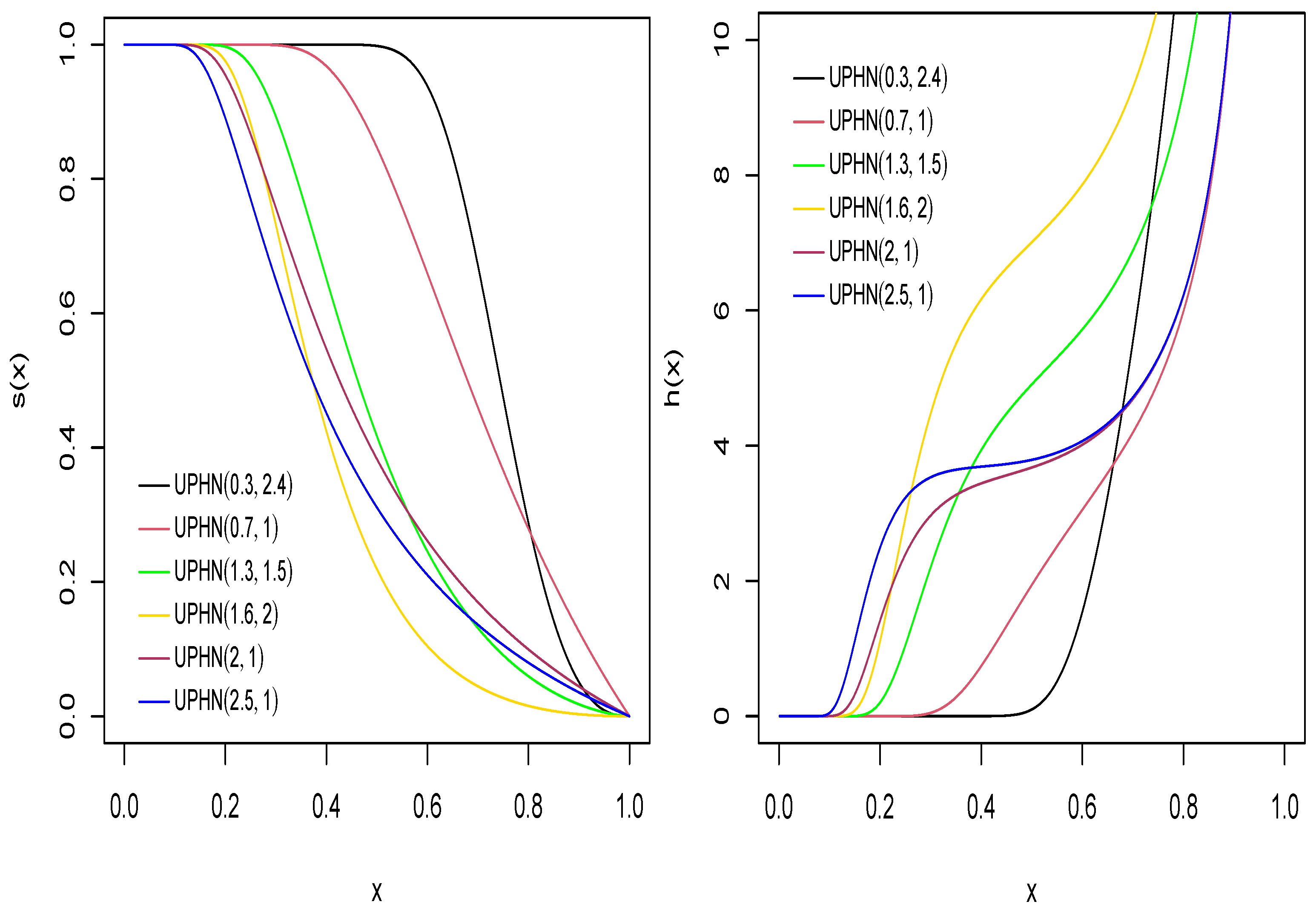
Figure 3 shows the survival and the hazard function for the UPHN$(\sigma ,\alpha )$ model, considering several values of $\sigma$ and $\alpha$. We highlight that the hazard function is increasing.

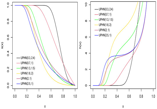
Figure 3. Survival and hazard functions for $\mathrm{U}\mathrm{P}\mathrm{H}\mathrm{N}(\sigma ,\alpha )$ model for some values of parameters $\sigma$ and $\alpha$.

2.3. Moments

Proposition 4.

Let $X\sim UPHN(\sigma ,\alpha )$. Then, the n-th moment of X, where n is a positive integer, is given by:

$${\mu }_X=\alpha b_n(\sigma ,\alpha ),$$

(7)

where ${\displaystyle b_n(\sigma ,\alpha )={\int }_0^1{\left(\sigma {\Phi }^{-1}\left(\frac{u+1}{2}\right)+1\right)}^{-n}{u}^{\alpha -1}du}$, are computed numerically.

Proof. 

The moments are immediately obtained from their definition.

$$\begin{array}{ccc}\hfill E\left[X^n\right]& =& {\displaystyle \frac{2\alpha }{\sigma }{\int }_0^1{x}^{n-2}\varphi \left(\frac{1-x}{\sigma x}\right){\left(2\Phi \left(\frac{1-x}{\sigma x}\right)-1\right)}^{\alpha -1}dx.}\hfill \end{array}$$

(8)

Making the change of variable ${\displaystyle u=2\Phi \left(\frac{1-x}{\sigma x}\right)-1}$, we have that:

$$\begin{array}{c}\hfill E\left[X^n\right]=\alpha {\int }_0^1{\left(\sigma {\Phi }^{-1}\left({\displaystyle \frac{u+1}{2}}\right)+1\right)}^{-n}{u}^{\alpha +1}du,\end{array}$$

and defining $b_n(\sigma ,\alpha )$ as the integral, the result is obtained.    □

Corollary 1.

Let $X\sim UPHN(\sigma ,\alpha )$. Then, the skewness $\left(\sqrt{{\mathit{\beta }}_1}\right)$ and kurtosis $\left({\mathit{\beta }}_2\right)$ coefficients are

$$\begin{array}{ccc}\hfill \sqrt{{\mathit{\beta }}_1}& =& {\displaystyle \frac{b_3-3b_1{b}_2+2b_1^3}{{(b_2-b_1^2)}^{3/2}}}and{\mathit{\beta }}_2={\displaystyle \frac{b_4-4b_1{b}_3+6b_1^2{b}_2-3b_1^4}{{(b_2-b_1^2)}^2}},\hfill \end{array}$$

where $b_n=b_n(\sigma ,\alpha )$.

Proof. 

It is immediately obtained from the definition of these coefficients.    □

Table 1 and Table 2 provide us $\left(\sqrt{{\mathit{\beta }}_1}\right)$ and $\left({\mathit{\beta }}_2\right)$ for several values of parameters $\sigma$ and $\alpha$. We can observe that for low values of $\sigma$ and $\alpha$, the skewness coefficient is negative and for high values, positive skewness is obtained. As for the kurtosis coefficient, the observed effect is more dispersed.

Table 1. Skewness coefficient of $\mathrm{U}\mathrm{P}\mathrm{H}\mathrm{N}(\sigma ,\alpha )$ model for different values of $\sigma$ and $\alpha$.

	$\mathit{\alpha }$
$\mathbf{\sigma }$	0.3	0.7	1.5	3	5
0.1	−1.7390	−0.9557	−0.5196	−0.3301	−0.2892
0.6	−1.1043	−0.3191	0.1764	0.3817	0.3805
1.4	−0.7097	0.1218	0.7115	0.9300	0.8517
2.5	−0.4381	0.4597	1.1669	1.3915	1.2040
5	−0.1228	0.9035	1.8445	2.0545	1.6279
10	0.1805	1.4033	2.7419	2.8675	2.0197

Table 2. Kurtosis coefficient of $\mathrm{U}\mathrm{P}\mathrm{H}\mathrm{N}(\sigma ,\alpha )$ model for different values of $\sigma$ and $\alpha$.

	$\mathit{\alpha }$
$\mathbf{\sigma }$	0.3	0.7	1.5	3	5
0.1	5.8356	3.4239	2.8539	2.8706	2.9599
0.6	3.1896	2.0788	2.3258	2.8454	3.0395
1.4	2.1877	1.8542	2.9189	4.0065	4.1003
2.5	1.7492	2.0303	4.0774	5.8378	5.5157
5	1.4777	2.6956	6.9298	10.0505	8.0999
10	1.4435	4.0179	12.8648	18.3334	11.6586

2.4. Incomplete Moments

The k-th incomplete moments of the UPHN distribution are given by:

$$\begin{array}{ccc}\hfill T_k\left(t\right)& =& E\left(X^k|x<t\right)\hfill \\ & =& {\displaystyle \frac{2\alpha }{\sigma }}{\int }_0^t{x}^{k-2}\varphi \left({\displaystyle \frac{1-x}{\sigma x}}\right){\left(2\Phi \left({\displaystyle \frac{1-x}{\sigma x}}\right)-1\right)}^{\alpha -1}dx,k=0,1,2,\dots \hfill \end{array}$$

This integral cannot be solved analytically. In particular, for $k=0,1,2$, we have:

$$\begin{array}{c}\hfill T_0\left(t\right)=F(t;\sigma ,\alpha ),T_1\left(t\right)=\alpha {\gamma }_1\left(a\left(t\right)\right),T_2\left(t\right)=\alpha {\gamma }_2\left(a\left(t\right)\right),\end{array}$$

where ${\displaystyle {\gamma }_j\left(a\left(t\right)\right)={\int }_{a\left(t\right)}^1{\left(\alpha {\Phi }^{-1}\left(\frac{u+1}{2}\right)+1\right)}^{-j}{u}^{\alpha -1}du}$ and $a\left(y\right)=2\Phi \left({\displaystyle \frac{1-y}{\sigma y}}\right)-1$. ${\gamma }_j\left(a\left(t\right)\right)$, are computed numerically.

2.5. The Lorenz Curve and the Gini Index

The standard definition of the Lorenz curve [17] is provided in terms of the first incomplete moment and the expected value of X. Specifically, for the UPHN model, the following closed form expression is obtained

$$\begin{array}{ccc}\hfill L\left(p\right)& =& {\displaystyle \frac{1}{{\mu }_X}}{\int }_0^{t}xf\left(x\right)dx={\displaystyle \frac{1}{{\mu }_X}}{T}_1\left(t\right);\hfill \\ & =& {\displaystyle \frac{\alpha }{{\mu }_X}}{\gamma }_1\left(a\left(t\right)\right).\hfill \end{array}$$

The Gini index, also known as the Gini coefficient (see [18,19]), is a statistical dispersion metric associated with the Lorenz curve, intended to represent income inequality, wealth inequality, or consumption inequality within a nation or social group. The Gini index is defined as:

$$\begin{array}{c}\hfill G(\sigma ,\alpha )=1-{\displaystyle \frac{1}{{\mu }_X}}{\int }_0^{\infty }{\left[1-T_0\left(t\right)\right]}^{2}dt.\end{array}$$

Proposition 5.

Let $X\sim UPHN(\sigma ,\alpha )$. Then, the Gini index is given by:

$$\begin{array}{ccc}\hfill G(\sigma ,\alpha )& =& 1-{\displaystyle \frac{4^{\alpha }}{{\mu }_X}}{\int }_0^{\infty }{\left[\Phi \left({\displaystyle \frac{1-t}{\sigma t}}\right)\right]}^{2\alpha }dt.\hfill \end{array}$$

Proof. 

By definition, the proof is direct.    □

Proposition 6.

Let $X\sim UPHN(\sigma ,\alpha )$; the Renyi entropy of order δ for X is given by:

$$\begin{array}{c}\hfill R_{\delta }\left(x\right)={\displaystyle \frac{1}{1-\delta }}\left(\delta log\left(\alpha \right)-log((\alpha -1)\delta +1)+log\left(1-{\left(1-2\Phi (1/\sigma )\right)}^{(\alpha -1)\delta +1}\right)\right),\end{array}$$

where $\delta >0$ and $\delta \ne 1$.

Proof. 

The Renyi entropy is defined as ${\displaystyle R_{\delta }\left(x\right)=\frac{1}{1-\delta }log\left({\int }_0^{\infty }f{\left(x\right)}^{\delta }dx\right)}$. Therefore, we have:

$$\begin{array}{c}\hfill R_{\delta }\left(y\right)={\displaystyle \frac{1}{1-\delta }}log\left({\int }_0^{\infty }{\left({\displaystyle \frac{2\alpha }{\sigma x^2}}\varphi \left({\displaystyle \frac{1-x}{\sigma x}}\right){\left(2\Phi \left({\displaystyle \frac{1-x}{\sigma x}}\right)-1\right)}^{\alpha -1}\right)}^{\delta }dx\right),\end{array}$$

Making the change of variable ${\displaystyle u=2\Phi \left(\frac{1-x}{\sigma x}\right)-1}$, the result is obtained.    □

2.6. Shannon Entropy

The entropy of a random variable X is a measure of its uncertainty. The Shannon entropy measure is defined by:

$$\begin{array}{c}\hfill {\mathbf{J}}_S=-E\left(log\left(f\right(x\left)\right)\right).\end{array}$$

If follows, after extensive algebraic manipulations, that the Shannon entropy for the UPHN model is:

$$\begin{array}{c}\hfill {\mathbf{J}}_S=log\left({\displaystyle \frac{\sigma \sqrt{2\pi }}{2\alpha }}\right)+2m_1+{\displaystyle \frac{1}{2{\sigma }^2}}\left(\alpha b_2(\sigma ,\alpha )-2\alpha b_1(\sigma ,\alpha )+1\right)+(\alpha +1)m_2.\end{array}$$

where $m_1=E(log\left(x\right))$, $m_2=E(log\left({\displaystyle 2\Phi \left(\frac{1-x}{\sigma x}\right)-1)}\right)$, and with $b_1(\sigma ,\alpha )$ and $b_2(\sigma ,\alpha )$ as given above.

2.7. Quantiles

Proposition 7.

Let $X\sim UPHN(\sigma ,\alpha )$. Then, the quantile function is given by:

$$Q(p;\sigma ,\alpha )={\left[\sigma {\Phi }^{-1}\left({\displaystyle \frac{{(1-p)}^{1/\alpha }}{2}}+{\displaystyle \frac{1}{2}}\right)+1\right]}^{-1},0<p<1.$$

(9)

Proof. 

It follows from a direct computation, by applying the definition of quantile function.    □

Corollary 2.

The quartiles for the $UPHN$ distribution are:

1. 

(First quartile) $Q(0.25;\sigma ,\alpha )={\left[\sigma {\Phi }^{-1}\left({\displaystyle \frac{0.{75}^{1/\alpha }}{2}+\frac{1}{2}}\right)+1\right]}^{-1}$.

2. 

(Median) $Q(0.5;\sigma ,\alpha )={\left[\sigma {\Phi }^{-1}\left({\displaystyle \frac{0.5^{1/\alpha }}{2}+\frac{1}{2}}\right)+1\right]}^{-1}$.

3. 

(Third quartile) $Q(0.75;\sigma ,\alpha )={\left[\sigma {\Phi }^{-1}\left({\displaystyle \frac{0.{25}^{1/\alpha }}{2}+\frac{1}{2}}\right)+1\right]}^{-1}$.

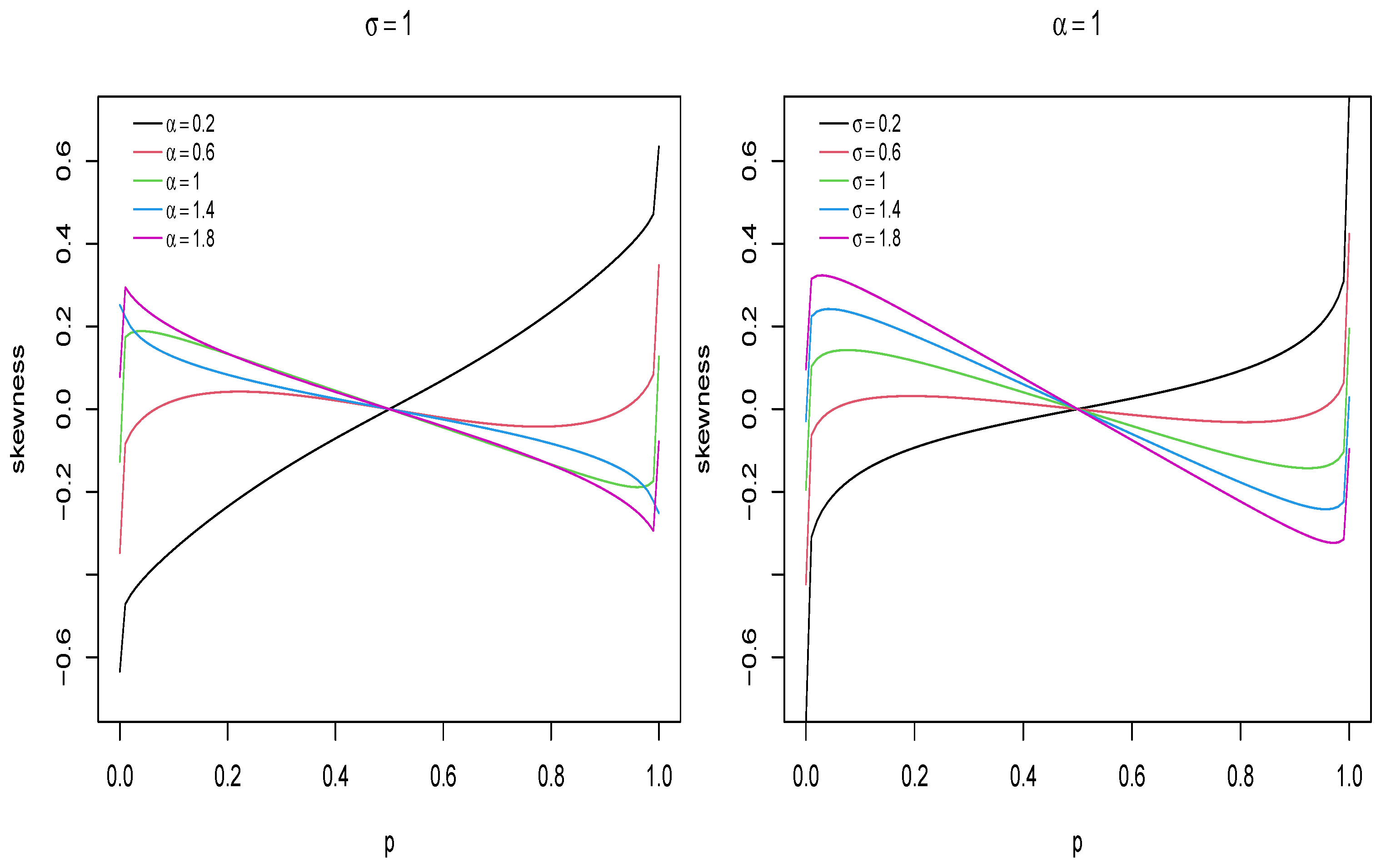
The quantile function can also be used to study the kurtosis and skewness in the UPHN model. A classical measurement for skewness was introduced by MacGillivray [20], which is given by:

$$\begin{array}{c}\hfill {\rho }_{X_i}\left(p\right)={\displaystyle \frac{Q_{X_i}(1-p;\sigma ,\alpha )+Q_{X_i}(p;\sigma ,\alpha )-2Q_{X_i}(0.5;\sigma ,\alpha )}{Q_{X_i}(1-p;\sigma ,\alpha )-Q_{X_i}(p;\sigma ,\alpha )}},p\in (0,1).\end{array}$$

(10)

In particular, the MacGuillevray skewness measurement can efficiently describe the effect of the parameters $(\sigma ,\alpha )$ on asymmetry. In Figure 4, the behavior of the asymmetry coefficient is plotted with respect to the values of the parameters.

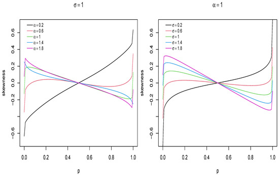
Figure 4. Plots of the MacGillivray skewness coefficient in UPHN model.

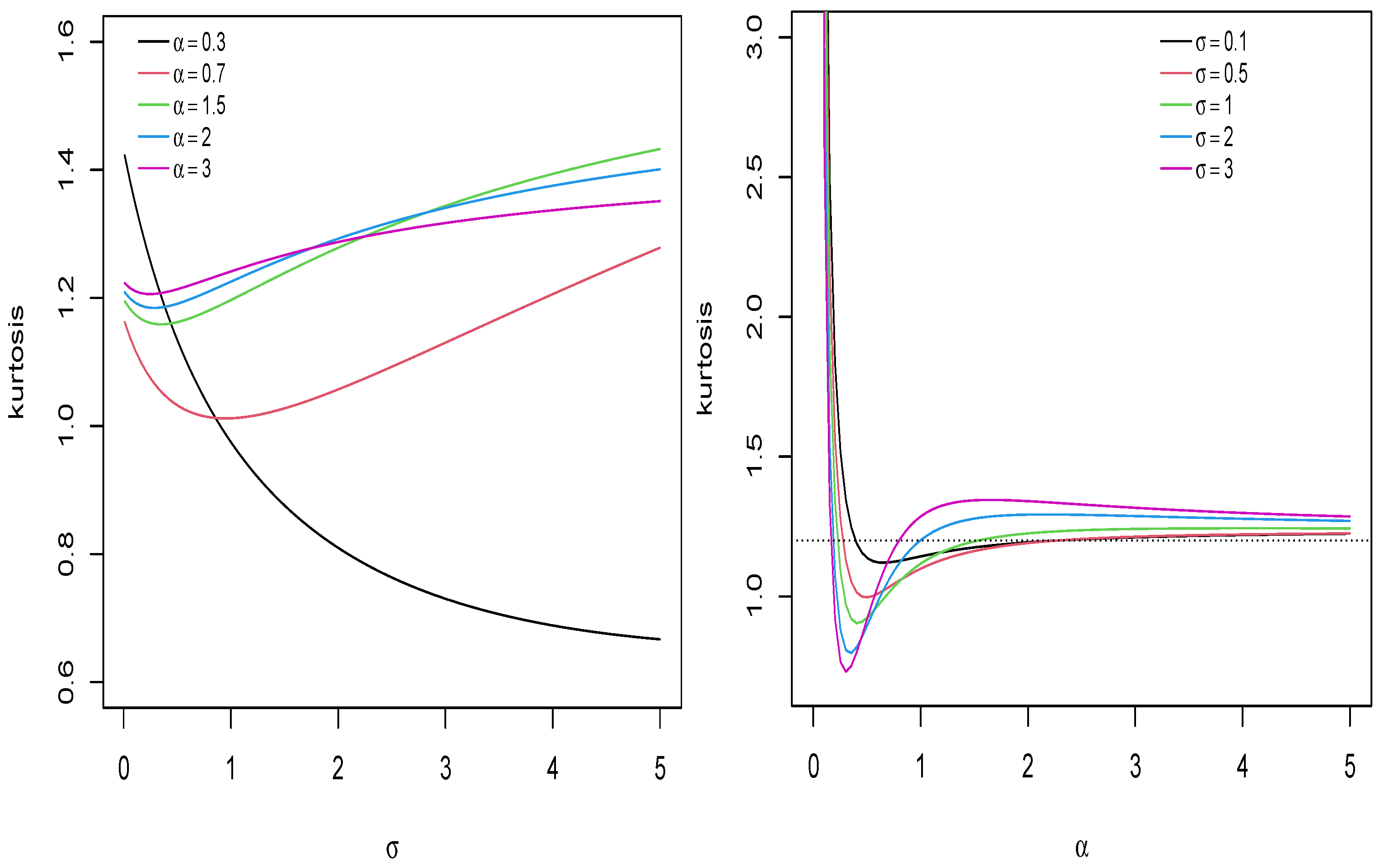
The kurtosis of the UPHN$(\sigma ,\alpha )$ distribution can also be studied using the Moors kurtosis coefficient [21], usually given by:

$$\begin{array}{c}\hfill K(\sigma ,\alpha )={\displaystyle \frac{Q(7/8;\sigma ,\alpha )-Q(5/8;\sigma ,\alpha )+Q(3/8;\sigma ,\alpha )-Q(1/8;\sigma ,\alpha )}{Q(3/4;\sigma ,\alpha )-Q(1/4;\sigma ,\alpha )}}.\end{array}$$

(11)

It can be seen in [21] that for large values of (11), the distribution has heavy tails and for small values, the model has lighter tails. Figure 5 shows the behavior of the Moors kurtosis coefficient for the UPHN distribution.

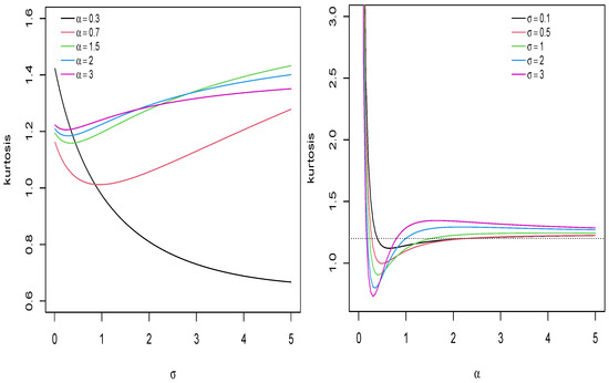
Figure 5. Plots of the Moors kurtosis coefficient for the $\mathrm{U}\mathrm{P}\mathrm{H}\mathrm{N}$ model.

2.8. Order Statistics

Order statistics have a wide range of applications in physical and life sciences (see, for instance, Balakrishnan and Cohen [22]). From a statistical perspective, they allow the computation of useful functions such as the sample range and the sample median. The following result states the pdf of k-th order statistic from a UPHN random sample of size n, which is arranged in a non-decreasing order.

Proposition 8.

Let $X_1,X_2,\dots ,X_n$ be independent and identically distributed $UPHN(\sigma ,\alpha )$ random variables. Then, the pdf of the k-th order statistic, $X_{k:n}$, is given by:

$$\begin{array}{c}\hfill {\displaystyle f_{X_{k:n}}\left(x\right)=\frac{2\alpha n!}{(k-1)!(n-k)!\sigma x^2}\varphi \left({\displaystyle \frac{1-x}{\sigma x}}\right){\left(2\Phi \left(\frac{1-x}{\sigma x}\right)-1\right)}^{\alpha (n-k+1)-1}{\left[1-{\left(2\Phi \left({\displaystyle \frac{1-x}{\sigma x}}\right)-1\right)}^{\alpha }\right]}^{k-1}.}\end{array}$$

Corollary 3.

Let $X_1,X_2,\dots ,X_n$ be a random sample from a $UPHN(\sigma ,\alpha )$ distribution. Then,

1. 

The pdf of the minimum, $X_{1:n}$, is

$$\begin{array}{ccc}\hfill f_{X_{1:n}}\left(x\right)& =& {\displaystyle \frac{2\alpha n}{\sigma x^2}\varphi \left({\displaystyle \frac{1-x}{\sigma x}}\right){\left(2\Phi \left(\frac{1-x}{\sigma x}\right)-1\right)}^{n\alpha -1},}\hfill \end{array}$$

2. 

The pdf of the maximum, $X_{n:n}$, is

$$\begin{array}{ccc}\hfill f_{X_{n:n}}\left(x\right)& =& {\displaystyle \frac{2\alpha n}{\sigma x^2}\varphi \left({\displaystyle \frac{1-x}{\sigma x}}\right){\left(2\Phi \left(\frac{1-x}{\sigma x}\right)-1\right)}^{\alpha -1}{\left[1-{\left(2\Phi \left({\displaystyle \frac{1-x}{\sigma x}}\right)-1\right)}^{\alpha }\right]}^{n-1}.}\hfill \end{array}$$

2.9. Bonferroni Curve

In various disciplines, such as socioeconomics and public health sciences, there is a need to compare and analyze inequality in distributions. Bonferroni curves are tools useful to reach this aim. It is worth mentioning that these curves have applications not only in economics to study income and poverty, but also in medicine or reliability. A detailed discussion can be seen in Bonferroni [23] or Arcagni and Porro [24]. The expressions of these curves for the UPHN model are presented below.

Proposition 9.

Let $X\sim UPHN(\sigma ,\alpha )$. Then, for $0<p<1,$ the Bonferroni curve, say $B\left(p\right)$, is given by:

$$\begin{array}{ccc}\hfill B\left(p\right)& =& {\displaystyle \frac{\alpha }{{\mu }_{X}p}}\sum _{j=0}^{\infty }{(-1)}^j{\sigma }^j{\gamma }_{a\left(q\right)}^j,\hfill \end{array}$$

where ${\mu }_X=E\left(X\right)$.

Proof. 

The expression above is obtained by using the definition of the Bonferroni curve, that is,

$${\displaystyle B\left(p\right)=\frac{1}{{\mu }_{X}p}{\int }_0^p{F}^{-1}\left(t\right)dt=\frac{1}{{\mu }_{X}p}{\int }_0^{q}xf\left(x\right)dx,0<p<1,}$$

where ${\mu }_X$ is the expected value of the corresponding non-negative random variable and $q=F^{-1}\left(p\right)$.    □

3. Inference

In this section, the inference about the parameters in the UPHN distribution is carried out from a classical point of view. Let us consider $X_1,X_2,\dots ,X_n$ a random sample of X∼$UPHN(\sigma ,\alpha )$. The maximum likelihood (ML) estimation method is discussed below. Given a random sample $x_1,x_2,\dots ,x_n$ of size n from $UPHN(\sigma ,\alpha )$, the log-likelihood function is given by:

$$\begin{array}{c}\hfill {\displaystyle \ell \left(\mathit{\theta }\right)=nlog\left(\frac{2\alpha }{\sigma }\right)-\frac{n}{2}log\left(2\pi \right)-2\sum _{i=1}^{n}log\left(x_i\right)-\frac{1}{2}\sum _{i=1}^n{v}_i^2+(\alpha -1)\sum _{i=1}^{n}log\left(2\Phi \left(v_i\right)-1\right),}\end{array}$$

(12)

where ${\displaystyle v_i=\frac{1-x_i}{\sigma x_i}}$. Therefore, the score assumes the form $S\left(\mathit{\theta }\right)=(S_{\sigma }\left(\mathit{\theta }\right),S_{\alpha }\left(\mathit{\theta }\right))$ where:

$$\begin{array}{ccc}\hfill S_{\sigma }\left(\mathit{\theta }\right)& =& {\displaystyle -\frac{n}{{\sigma }^2}+\frac{1}{\sigma }\sum _{i=1}^n{v}_i^2-\frac{2(\alpha -1)}{\sigma }\sum _{i=1}^n\frac{\varphi \left(v_i\right)v_i}{2\Phi \left(v_i\right)-1},}\hfill \end{array}$$

(13)

$$\begin{array}{ccc}\hfill S_{\alpha }\left(\mathit{\theta }\right)& =& {\displaystyle \frac{n}{\alpha }}+\sum _{i=1}^{n}log\left(2\Phi \left(v_i\right)-1\right).\hfill \end{array}$$

(14)

The ML estimators (MLEs) can be obtained by solving the likelihood Equations (13) and (14). Numerical methods, such as the Newton–Raphson procedure, must be used. Alternative maximization techniques could also be applied, for instance, those proposed in MacDonald [25].

The asymptotic variance of the MLEs, say $\widehat{\mathit{\theta }}=(\widehat{\sigma },\widehat{\alpha })$, can be estimated by the Fisher information matrix defined as $\mathcal{I}\left(\mathit{\theta }\right)=-\mathbb{E}\left[{\partial }^2\ell \left(\mathit{\theta }\right)/\partial \mathit{\theta }\partial {\mathit{\theta }}^{\top }\right]$, where $\ell \left(\mathit{\theta }\right)$ is the log-likelihood function of the UPHN model given in (12). Recall that, under the regularity conditions,

$$\mathcal{I}{\left(\mathit{\theta }\right)}^{-1/2}\left(\widehat{\mathit{\theta }}-\mathit{\theta }\right)\stackrel{\mathcal{D}}{\to }{N}_2({\mathbf{0}}_2,{\mathit{I}}_2),asn\to +\infty ,$$

where $\mathcal{D}$ stands for convergence in distribution and $N_2({\mathbf{0}}_2,{\mathit{I}}_2)$ denotes the standard bivariate normal distribution. The elements of the matrix $-{\partial }^2\ell \left(\mathit{\theta }\right)/\partial \mathit{\theta }\partial {\mathit{\theta }}^{\top }$ are given by $I_{\sigma \sigma }=-{\partial }^2\ell \left(\mathit{\theta }\right)/\partial {\sigma }^2$, $I_{\sigma \alpha }=-{\partial }^2\ell \left(\mathit{\theta }\right)/\partial \sigma \partial \alpha$ and $I_{\alpha \alpha }=-{\partial }^2\ell \left(\mathit{\theta }\right)/\partial {\alpha }^2$. Explicitly, we have:

$$\begin{array}{ccc}\hfill I_{\sigma \sigma }& =& -{\displaystyle \frac{n}{{\sigma }^2}}+{\displaystyle \frac{3}{{\sigma }^2}}\sum _{i=1}^n{v}_i^2-{\displaystyle \frac{4(\alpha -1)}{{\sigma }^2}}\sum _{i=1}^n{\displaystyle \frac{\varphi \left(v_i\right)v_i}{2\Phi \left(v_i\right)-1}}+{\displaystyle \frac{2(\alpha -1)}{{\sigma }^2}}\sum _{i=1}^n{\displaystyle \frac{v_i^2\varphi \left(v_i\right)\left[v_i(2\Phi \left(v_i\right)-1)+2\varphi \left(v_i\right)\right]}{{(2\varphi \left(v_i\right)-1)}^2}},\hfill \\ \hfill I_{\sigma \alpha }& =& -{\displaystyle \frac{2}{{\sigma }^2}}\sum _{i=1}^n{\displaystyle \frac{v_i\varphi \left(v_i\right)}{2\Phi \left(v_i\right)-1}},\hfill \\ \hfill I_{\alpha \alpha }& =& {\displaystyle \frac{n}{{\alpha }^2}}.\hfill \end{array}$$

In practice, it is not possible to obtain in a closed form the expected value of previous expressions. However, the covariance matrix of the MLEs, $\mathcal{I}{\left(\mathit{\theta }\right)}^{-1}$, can be estimated consistently by $I{\left(\widehat{\mathit{\theta }}\right)}^{-1}$, where $I\left(\widehat{\mathit{\theta }}\right)$ denotes the observed information matrix, which is obtained as

$$I\left(\widehat{\mathit{\theta }}\right)=-{\displaystyle \frac{{\partial }^2\ell \left(\mathit{\theta }\right)}{\partial \mathit{\theta }\partial {\mathit{\theta }}^{\top }}}{|}_{\mathit{\theta }=\widehat{\mathit{\theta }}}.$$

The asymptotic variances of $\widehat{\sigma }$ and $\widehat{\alpha }$ are estimated by the diagonal elements of $I{\left(\widehat{\mathit{\theta }}\right)}^{-1}$, and their standard errors by the square root of asymptotic variances.

4. Quantile Regression

We now introduce a regression study, in which a quantile regression model is proposed to describe the conditional quantile of the response variable. Given the quantile function of the $UPHN$ distribution, the pdf of the UPHN distribution can be reparameterized in terms of its $p^{th}$ quantile, denoted as $\rho =Q(p;\sigma ,\alpha )$.

Let ${\displaystyle \sigma =\frac{1-\rho }{\rho {\Phi }^{-1}\left(\frac{1}{2}\left({(1-p)}^{1/\alpha }+1\right)\right)}}$. Then, the reparameterized pdf for the UPHN model is:

$$\begin{array}{c}\hfill f_X(x;\rho ,\alpha ,p)={\displaystyle \frac{2\alpha }{(1-\alpha )x^2}}h(\alpha ,p)\varphi \left({\displaystyle \frac{(1-x)\rho }{(1-\rho )x}}h(\alpha ,p)\right){\left(2\Phi \left({\displaystyle \frac{(1-x)\rho }{(1-\rho )x}}h(\alpha ,p)\right)-1\right)}^{\alpha -1},\end{array}$$

(15)

where $h(\alpha ,p)={\Phi }^{-1}\left({\displaystyle \frac{1}{2}}\left({(1-p)}^{1/\alpha }+1\right)\right)$, $0<x<1$, $0<p<1$, $0<\rho <1$, and $\alpha >0$.

The cdf of the reparameterized UPHN distribution is:

$$F(x;\rho ,\alpha ,p)=1-{\left[2\Phi \left({\displaystyle \frac{(1-x)\rho {\Phi }^{-1}\left(\frac{1}{2}[{(1-p)}^{1/\alpha }+1]\right)}{(1-\rho )x}}\right)-1\right]}^{\alpha }.$$

4.1. Model Formulation

Let us suppose that $0<p<1$ is fixed and we have a random sample $x_i\left(p\right)$∼$\mathrm{U}\mathrm{P}\mathrm{H}\mathrm{N}({\rho }_i,\alpha )$, $i=1,2,\dots ,n$. Here, the parameters ${\rho }_i$ and $\alpha$ are unknown. As a result, the suggested quantile regression model can be defined as:

$$\begin{array}{c}\hfill g\left({\rho }_i\left(p\right)\right)={\mathit{z}}_{\mathit{i}}^{\top }\mathit{\beta }\left(\mathit{p}\right),\end{array}$$

(16)

where ${\mathit{\beta }}^{\top }\left(p\right)=({\beta }_0\left(p\right),{\beta }_1\left(p\right),\dots ,{\beta }_k\left(p\right))$ and ${\mathit{z}}_{\mathit{i}}^{\top }=(1,z_{i1},\dots ,z_{ik})$ act as the regression coefficient vector and the ith vector of covariate values, respectively. It is important to note that g is the link function that associates the covariates with the response variable. We can obtain a median quantile regression for a unit response variable when $p=0.5$. Taking into account that the UPHN distribution is a probability model with support on $(0,1)$, we use and define the logit-link function as:

$$\begin{array}{c}\hfill g\left({\rho }_i\left(p\right)\right)=log\left({\displaystyle \frac{{\rho }_i\left(p\right)}{1-{\rho }_i\left(p\right)}}\right),i=1,\dots ,n.\end{array}$$

(17)

4.2. ML Method for the Regression Coefficients

Now, our objective is to estimate the unknown parameters of the UPHN quantile regression model using the ML technique. For this purpose, the logit link function is considered:

$$\begin{array}{c}\hfill g\left({\rho }_i\left(p\right)\right)=log\left({\displaystyle \frac{{\rho }_i\left(p\right)}{1-{\rho }_i\left(p\right)}}\right)={\mathit{z}}_{\mathit{i}}^{\top }\mathit{\beta }.\end{array}$$

(18)

From the above formula, the inverse link function is:

$$\begin{array}{c}\hfill {\rho }_i\left(p\right)={\displaystyle \frac{exp\left({\mathit{z}}_{\mathit{i}}^{\top }\mathit{\beta }\left(p\right)\right)}{1+exp\left({\mathit{z}}_{\mathit{i}}^{\top }\mathit{\beta }\left(p\right)\right)}}.\end{array}$$

(19)

Let us now have a random sample $X_1,\dots ,X_n$ with $X_i\sim \mathrm{UPNH}({\rho }_i\left(p\right),\alpha )$, and observed values $x_1,\dots ,x_n$. Then, using the pdf introduced in (15), the associated log-likelihood function is:

$$\begin{array}{ccc}\hfill l\left(\mathbf{\Theta }\right(p\left)\right)& =& n\left[log\left(2\right)+log\left(\alpha \right)\right]+nlog\left[h(\alpha ,p)\right]+\sum _{i=1}^{n}log\left[\varphi \left({\displaystyle \frac{[1-x_i]{\rho }_i}{[1-{\rho }_i]x_i}h(\alpha ,p)}\right)\right]\hfill \\ & +& \sum _{i=1}^{n}log\left({\displaystyle \frac{{\rho }_i}{[1-{\rho }_i]x_i^2}}\right)+(\alpha -1)\sum _{i=1}^{n}log\left[2\Phi \left({\displaystyle \frac{[1-x_i]{\rho }_i}{[1-{\rho }_i]x_i}h(\alpha ,p)}\right)-1\right],\hfill \end{array}$$

(20)

where $\mathrm{\Theta }={(\alpha ,{\mathit{\beta }}^{\top })}^{\top }$ denotes the unknown vector of parameters. The ML estimators of $\mathrm{\Theta }$, denoted as $\widehat{\mathrm{\Theta }}={(\widehat{\alpha },{\widehat{\mathit{\beta }}}^{\top })}^{\top }$ is achieved by maximizing $l\left(\mathbf{\Theta }\right)$ with respect to $\mathrm{\Theta }$. The optim function of the R software, 4.3.1 version, [26] can be used to maximize $l\left(\mathbf{\Theta }\right)$.

4.3. Model Checking

Once we have fitted the model, it is crucial to assess whether the regression model is appropriate for the data. In this sense, the analysis of residuals is key to check or validate the fitted model. We focus on the Cox–Snell residuals (Cox and Snell 1968) [27], which are calculated for the $ith$ observation as:

$${\widehat{\eta }}_i=-log\left[1-F(x_i;{\rho }_i\left(p\right),\alpha )\right],i=1,\dots ,n.$$

Here, $F(x_i,{\rho }_i\left(p\right),\alpha )$ stands for the estimated cdf of the UPHN distribution reparameterized in terms of quantiles. If the fitted model provides a good fit for the data, the residual ${\widehat{\eta }}_i$ will be an observation of a random variable from an exponential distribution with a scale parameter of one.

5. Simulation

In this section, a simulation study is carried out to evaluate the performance of the ML estimators. We used R software 4.3.1 version, for our calculations, developing customized code that integrates the optim function from R package stats [28].

5.1. Simulation 1

Next, an algorithm to generate samples from the $\mathrm{UPHN}(\sigma ,\alpha )$ is provided. Algorithm 1 is based on the inverse transformation method, where the inverse of the cdf is used.

Algorithm 1 Simulating values from the $\mathrm{UPHN}(\sigma ,\alpha )$ distribution.

1: Simulate $U\sim U(0,1)$. 2: Calculate $X={\left[\sigma {\Phi }^{-1}\left({\displaystyle \frac{{(1-U)}^{1/\alpha }}{2}}+{\displaystyle \frac{1}{2}}\right)+1\right]}^{-1}$

As parameter values in our simulation, we consider $\sigma \in \left\{1,2\right\}$ and $\alpha \in \left\{0.8,1,2,3,5\right\}$. For the sample size, we consider $n\in \left\{150,300,600\right\}$. For each sample size and every combination of $\sigma$, $\alpha$, we perform 1000 repetitions and the corresponding ML estimates are calculated. The results are given in Table 3. As summaries, we provide the estimated bias (bias) for the ML estimators of $\sigma$ and $\alpha$, standard errors (SE), the root of the estimated mean square error (RMSE), and the empirical coverage probability (CP) for the asymptotic intervals based on MLEs to 95%. For the ML estimators of $\sigma$ and $\alpha$, it should be noted that, as the sample size increases, the bias, SE, and RMSE decrease. It should also be noted that as the sample size increases, the SE and RMSE are closer, which suggests that the standard errors of the ML estimators are well estimated. As for the CPs, we highlight that they are close to the nominal level 0.95.

Table 3. Estimated bias, SE, and RMSE for ML estimators in finite samples from the $UPHN$ model.

True Value			$\mathit{n}=150$				$\mathit{n}=300$				$\mathit{n}=600$
$\mathit{\sigma }$	$\mathit{\alpha }$	Estimator	Bias	se	RMSE	CP	Bias	se	RMSE	CP	Bias	se	RMSE	CP
1	0.8	$\sigma$	−0.0075	0.0734	0.0747	0.930	−0.0036	0.0522	0.0520	0.948	−0.0013	0.0370	0.0364	0.947
		$\alpha$	0.0160	0.0774	0.0793	0.953	0.0084	0.0541	0.0549	0.955	0.0037	0.0380	0.0375	0.954
	1	$\sigma$	−0.0084	0.0680	0.0690	0.932	−0.0048	0.0482	0.0479	0.944	−0.0012	0.0343	0.0335	0.956
		$\alpha$	0.0181	0.0993	0.1028	0.946	0.0127	0.0697	0.0724	0.946	0.0017	0.0487	0.0490	0.949
	2	$\sigma$	−0.0027	0.0558	0.0554	0.944	0.0012	0.0397	0.0403	0.948	0.0001	0.0280	0.0293	0.933
		$\alpha$	0.0441	0.2229	0.2312	0.953	0.0083	0.1542	0.1555	0.951	0.0080	0.1090	0.1135	0.944
	3	$\sigma$	−0.0038	0.0507	0.0506	0.951	−0.0022	0.0359	0.0360	0.940	−0.0012	0.0254	0.0263	0.931
		$\alpha$	0.0718	0.3630	0.3601	0.971	0.0230	0.2514	0.2451	0.953	0.0211	0.1776	0.1811	0.942
	5	$\sigma$	−0.0050	0.0459	0.0463	0.945	−0.0020	0.0326	0.0334	0.938	−0.0004	0.0231	0.0240	0.937
		$\alpha$	0.1446	0.6799	0.7206	0.958	0.0678	0.4715	0.4976	0.948	0.0285	0.3300	0.3399	0.948
2	0.8	$\sigma$	−0.0089	0.1474	0.1461	0.954	−0.0080	0.1044	0.1044	0.948	−0.0029	0.0741	0.0748	0.941
		$\alpha$	0.0124	0.0770	0.0773	0.952	0.0060	0.0539	0.0553	0.952	0.0020	0.0379	0.0367	0.956
	1	$\sigma$	−0.0194	0.1358	0.1320	0.949	−0.0061	0.0967	0.0989	0.946	−0.0011	0.0687	0.0689	0.944
		$\alpha$	0.0169	0.0991	0.1021	0.953	0.0109	0.0696	0.0733	0.947	0.0014	0.0487	0.0491	0.948
	2	$\sigma$	−0.0050	0.1117	0.1097	0.946	−0.0049	0.0789	0.0771	0.953	−0.0022	0.0559	0.0570	0.942
		$\alpha$	0.0335	0.2215	0.2244	0.957	0.0218	0.1554	0.1548	0.951	0.0092	0.1091	0.1121	0.949
	3	$\sigma$	−0.0125	0.1009	0.0997	0.946	−0.0015	0.0719	0.0760	0.934	0.0007	0.0509	0.0511	0.942
		$\alpha$	0.0789	0.3638	0.3705	0.955	0.0238	0.2514	0.2534	0.955	0.0098	0.1767	0.1741	0.949
	5	$\sigma$	−0.0059	0.0921	0.0929	0.949	−0.0022	0.0652	0.0667	0.942	−0.0002	0.0462	0.0467	0.945
		$\alpha$	0.1166	0.6755	0.7079	0.947	0.0580	0.4702	0.4761	0.958	0.0204	0.3293	0.3392	0.943

5.2. Simulation 2

In this section, data are generated from the quantile regression model with sample sizes $n\in \{100,200,300,400\}$ and quantile levels $p\in \{0.10,0.25,0.50,0.75,0.90\}$ under two different scenarios. In the first scenario, three covariates are considered, that is,

$$\begin{array}{c}\hfill logit\left({\rho }_i\left(p\right)\right)={\beta }_0\left(p\right)+{\beta }_1\left(p\right)z_{i1}+{\beta }_2\left(p\right)z_{i2}+{\beta }_3\left(p\right)z_{i3},i=1,2,\dots ,n,\end{array}$$

(21)

where ${\beta }_0\left(p\right)=0.275,{\beta }_1\left(p\right)=0.098,{\beta }_2\left(p\right)=0.015,{\beta }_3\left(p\right)=0.397$, $z_{i1},z_{i2},z_{i3}\stackrel{\mathrm{iid}}{\sim }\mathrm{N}(0,1)$, and $\alpha =1.285$, whereas in the second scenario, five covariates are proposed

$$\begin{array}{c}\hfill logit\left({\rho }_i\left(p\right)\right)={\beta }_0\left(p\right)+{\beta }_1\left(p\right)z_{i1}+{\beta }_2\left(p\right)z_{i2}+{\beta }_3\left(p\right)z_{i3}+{\beta }_4\left(p\right)z_{i4}+{\beta }_5\left(p\right)z_{i5},\end{array}$$

(22)

where ${\beta }_0\left(p\right)=-2.975$, ${\beta }_1\left(p\right)=0.005$, ${\beta }_2\left(p\right)=0.092$, ${\beta }_3\left(p\right)=-0.958$, ${\beta }_4\left(p\right)=-0.122$, ${\beta }_5\left(p\right)=-0.289$, $z_{i1},z_{i2},z_{i3},z_{i4},z_{i5}\stackrel{\mathrm{iid}}{\sim }\mathrm{N}(0,1)$, and $\alpha =7.425$.

For fixed values of n and p, the response variable is generated as

$$\begin{array}{c}\hfill x_i={\left[{\sigma }_i{\Phi }^{-1}\left({\displaystyle \frac{{(1-u_i)}^{1/\alpha }}{2}}+{\displaystyle \frac{1}{2}}\right)+1\right]}^{-1},\end{array}$$

(23)

where $u_i$ is an observation generated from a continuous uniform distribution on $(0,1)$, that is, $u_i\sim U(0,1)$ and ${\sigma }_i$ is calculated as

$$\begin{array}{c}\hfill {\sigma }_i={\displaystyle \frac{1-{\rho }_i}{{\rho }_i{\Phi }^{-1}\left(\frac{1}{2}[{(1-p)}^{1/\alpha }+1]\right)}}.\end{array}$$

(24)

For both scenarios, and fixed $(n,p,\alpha )$, $M=500$ Monte Carlo replicates were performed. Then, the empirical bias, RMSE, and CP are calculated by

$$\begin{array}{cc}\hfill \mathrm{Bias}\left(\widehat{\gamma }\right)& ={\displaystyle \frac{1}{M}}\sum _{i=1}^M({\widehat{\gamma }}_i-\gamma ),\hfill \\ \hfill \mathrm{RMSE}\left(\widehat{\gamma }\right)& ={\left[{\displaystyle \frac{1}{M}}\sum _{i=1}^M{({\widehat{\gamma }}_i-\gamma )}^2\right]}^{1/2},\hfill \\ \hfill {\mathrm{CP}}_{95\%}& ={\displaystyle \frac{1}{M}}\sum _{i=1}^M{1}_{[{\widehat{\gamma }}_i\pm 1.96\times \mathrm{SE}\left({\widehat{\gamma }}_i\right)]}\left(\gamma \right),\hfill \end{array}$$

respectively, where $\gamma =\alpha ,{\beta }_j\left(p\right)$, $j=1,\dots ,5$, $1_{[{\widehat{\gamma }}_i\pm 1.96\times \mathrm{SE}\left({\widehat{\gamma }}_i\right)]}\left(\gamma \right)$ is the indicator function defined by

$$1_{[{\widehat{\gamma }}_i\pm 1.96\times \mathrm{SE}\left({\widehat{\gamma }}_i\right)]}\left(\gamma \right)=\left\{\begin{array}{cc}1,\hfill & \gamma \in ({\widehat{\gamma }}_i\pm 1.96\times \mathrm{SE}\left({\widehat{\gamma }}_i\right))\hfill \\ 0,\hfill & \gamma \notin ({\widehat{\gamma }}_i\pm 1.96\times \mathrm{SE}\left({\widehat{\gamma }}_i\right))\hfill \end{array}\right.,$$

and $\mathrm{SE}\left({\widehat{\gamma }}_i\right)$ is the estimated standard error of ${\widehat{\gamma }}_i$.

These summaries are provided in Table 4 and Table 5. In both settings, the good performance of our estimators is observed.

Table 4. Empirical bias, RMSE, and ${\mathrm{CP}}_{95\%}$ for the true values ${\beta }_0\left(p\right)=0.275$, ${\beta }_1\left(p\right)=0.098,{\beta }_2\left(p\right)=0.015$, ${\beta }_3\left(p\right)=0.397$, and $\alpha =1.285$ with simulated data.

p	n	Bias					RMSE					CP95%
		${\mathit{\beta }}_{\mathbf{0}}\left(\mathit{p}\right)$	${\mathit{\beta }}_{\mathbf{1}}\left(\mathit{p}\right)$	${\mathit{\beta }}_{\mathbf{2}}\left(\mathit{p}\right)$	${\mathit{\beta }}_{\mathbf{3}}\left(\mathit{p}\right)$	$\mathit{\alpha }$	${\mathit{\beta }}_{\mathbf{0}}\left(\mathit{p}\right)$	${\mathit{\beta }}_{\mathbf{1}}\left(\mathit{p}\right)$	${\mathit{\beta }}_{\mathbf{2}}\left(\mathit{p}\right)$	${\mathit{\beta }}_{\mathbf{3}}\left(\mathit{p}\right)$	$\mathit{\alpha }$	${\mathit{\beta }}_{\mathbf{0}}\left(\mathit{p}\right)$	${\mathit{\beta }}_{\mathbf{1}}\left(\mathit{p}\right)$	${\mathit{\beta }}_{\mathbf{2}}\left(\mathit{p}\right)$	${\mathit{\beta }}_{\mathbf{3}}\left(\mathit{p}\right)$	$\mathit{\alpha }$
0.1	100	0.018	0.000	0.000	−0.005	0.070	0.069	0.072	0.064	0.067	0.184	0.940	0.950	0.956	0.948	0.960
	200	0.011	−0.003	0.001	0.002	0.022	0.048	0.046	0.043	0.043	0.116	0.924	0.932	0.942	0.954	0.952
	300	0.005	−0.002	0.003	−0.001	0.015	0.037	0.035	0.037	0.039	0.096	0.944	0.964	0.948	0.940	0.958
	400	0.005	0.000	0.000	−0.001	0.014	0.034	0.034	0.032	0.034	0.081	0.940	0.950	0.950	0.952	0.958
0.25	100	0.012	−0.003	−0.004	0.000	0.073	0.072	0.060	0.059	0.071	0.190	0.918	0.942	0.936	0.944	0.952
	200	0.006	−0.002	0.000	−0.001	0.026	0.046	0.046	0.044	0.044	0.118	0.938	0.946	0.956	0.948	0.956
	300	0.005	0.001	−0.001	0.002	0.016	0.037	0.040	0.036	0.039	0.090	0.938	0.956	0.954	0.944	0.962
	400	0.001	0.001	−0.001	0.002	0.021	0.032	0.033	0.034	0.031	0.084	0.944	0.942	0.940	0.960	0.956
0.5	100	0.010	−0.006	−0.002	−0.006	0.057	0.079	0.065	0.064	0.075	0.188	0.940	0.944	0.944	0.934	0.950
	200	0.004	−0.001	0.001	−0.003	0.038	0.051	0.048	0.048	0.046	0.118	0.956	0.946	0.930	0.940	0.962
	300	0.002	0.005	0.001	−0.002	0.019	0.046	0.037	0.035	0.036	0.097	0.926	0.956	0.948	0.956	0.952
	400	−0.001	−0.001	0.000	−0.001	0.022	0.035	0.03	0.034	0.031	0.081	0.956	0.960	0.940	0.954	0.954
0.75	100	−0.007	0.001	−0.002	0.002	0.059	0.117	0.068	0.068	0.064	0.183	0.940	0.946	0.942	0.940	0.954
	200	0.001	0.002	−0.001	−0.002	0.027	0.082	0.041	0.044	0.047	0.122	0.950	0.944	0.946	0.938	0.958
	300	−0.004	−0.001	0.000	−0.002	0.024	0.066	0.036	0.035	0.040	0.094	0.954	0.958	0.966	0.926	0.956
	400	0.002	0.001	0.001	0.001	0.014	0.053	0.033	0.032	0.031	0.079	0.966	0.936	0.958	0.950	0.964
0.9	100	−0.031	0.000	0.001	0.004	0.067	0.196	0.070	0.066	0.065	0.198	0.920	0.944	0.952	0.936	0.940
	200	−0.020	0.001	0.000	0.004	0.035	0.140	0.050	0.043	0.044	0.123	0.928	0.944	0.942	0.964	0.954
	300	−0.008	−0.001	−0.001	0.000	0.019	0.113	0.038	0.039	0.039	0.097	0.942	0.948	0.958	0.936	0.948
	400	−0.004	−0.001	0.000	0.002	0.013	0.095	0.034	0.031	0.033	0.083	0.952	0.942	0.944	0.948	0.942

Table 5. Empirical bias, RMSE, and ${\mathrm{CP}}_{95\%}$ for the true values ${\beta }_0\left(p\right)=-2.975$, ${\beta }_1\left(p\right)=0.005$, ${\beta }_2\left(p\right)=0.092$, ${\beta }_3\left(p\right)=-0.958$, ${\beta }_4\left(p\right)=-0.122$, ${\beta }_5\left(p\right)=-0.289$, and $\alpha =7.425$ with simulated data.

p	n				Bias							RMSE							CP95%
		${\mathit{\beta }}_{\mathbf{0}}\left(\mathit{p}\right)$	${\mathit{\beta }}_{\mathbf{1}}\left(\mathit{p}\right)$	${\mathit{\beta }}_{\mathbf{2}}\left(\mathit{p}\right)$	${\mathit{\beta }}_{\mathbf{3}}\left(\mathit{p}\right)$	${\mathit{\beta }}_{\mathbf{4}}\left(\mathit{p}\right)$	${\mathit{\beta }}_{\mathbf{5}}\left(\mathit{p}\right)$	$\mathit{\alpha }$	${\mathit{\beta }}_{\mathbf{0}}\left(\mathit{p}\right)$	${\mathit{\beta }}_{\mathbf{1}}\left(\mathit{p}\right)$	${\mathit{\beta }}_{\mathbf{2}}\left(\mathit{p}\right)$	${\mathit{\beta }}_{\mathbf{3}}\left(\mathit{p}\right)$	${\mathit{\beta }}_{\mathbf{4}}\left(\mathit{p}\right)$	${\mathit{\beta }}_{\mathbf{5}}\left(\mathit{p}\right)$	$\mathit{\alpha }$	${\mathit{\beta }}_{\mathbf{0}}\left(\mathit{p}\right)$	${\mathit{\beta }}_{\mathbf{1}}\left(\mathit{p}\right)$	${\mathit{\beta }}_{\mathbf{2}}\left(\mathit{p}\right)$	${\mathit{\beta }}_{\mathbf{3}}\left(\mathit{p}\right)$	${\mathit{\beta }}_{\mathbf{4}}\left(\mathit{p}\right)$	${\mathit{\beta }}_{\mathbf{5}}\left(\mathit{p}\right)$	$\mathit{\alpha }$
0.1	100	0.009	0.001	0.000	−0.003	−0.001	0.001	0.844	0.038	0.034	0.030	0.031	0.029	0.030	1.745	0.928	0.936	0.960	0.946	0.944	0.956	0.964
	200	0.006	0.001	0.000	0.001	0.000	0.001	0.344	0.027	0.020	0.021	0.021	0.020	0.022	1.069	0.926	0.944	0.948	0.950	0.968	0.938	0.952
	300	0.003	0.000	0.000	0.000	0.000	0.000	0.210	0.020	0.018	0.019	0.018	0.017	0.017	0.829	0.942	0.936	0.924	0.964	0.958	0.954	0.958
	400	0.003	0.001	0.001	0.000	−0.001	−0.001	0.187	0.018	0.015	0.015	0.015	0.014	0.017	0.699	0.952	0.952	0.962	0.930	0.960	0.926	0.952
0.25	100	0.006	0.002	0.002	0.002	0.001	0.000	0.851	0.035	0.035	0.032	0.03	0.031	0.032	1.806	0.926	0.930	0.952	0.958	0.938	0.948	0.956
	200	0.002	0.000	0.000	0.001	0.001	0.001	0.341	0.023	0.021	0.024	0.024	0.023	0.023	1.053	0.946	0.944	0.926	0.942	0.938	0.942	0.968
	300	0.003	0.000	−0.001	−0.001	0.001	0.000	0.239	0.019	0.018	0.017	0.018	0.018	0.017	0.793	0.940	0.948	0.942	0.946	0.942	0.948	0.956
	400	0.001	0.000	0.001	0.000	−0.001	0.001	0.223	0.016	0.015	0.016	0.016	0.016	0.015	0.701	0.950	0.95	0.938	0.932	0.950	0.956	0.96
0.5	100	0.003	0.001	0.000	0.000	0.000	−0.002	0.783	0.032	0.031	0.035	0.028	0.033	0.027	1.698	0.936	0.948	0.916	0.954	0.938	0.942	0.974
	200	0.001	0.001	−0.001	0.002	0.001	−0.001	0.441	0.022	0.021	0.020	0.020	0.021	0.020	1.065	0.950	0.944	0.940	0.954	0.928	0.950	0.964
	300	0.001	0.000	0.000	0.000	−0.001	0.002	0.249	0.018	0.017	0.017	0.018	0.018	0.018	0.84	0.936	0.946	0.952	0.940	0.946	0.940	0.964
	400	−0.001	0.000	0.001	0.000	0.000	0.000	0.238	0.015	0.015	0.016	0.015	0.015	0.015	0.688	0.962	0.950	0.962	0.942	0.952	0.948	0.95
0.750	100	−0.003	−0.001	0.001	0.002	0.004	0.000	0.730	0.037	0.030	0.031	0.029	0.033	0.030	1.741	0.930	0.942	0.946	0.956	0.926	0.930	0.956
	200	−0.002	0.000	−0.001	−0.001	0.000	0.000	0.415	0.026	0.022	0.022	0.022	0.022	0.021	1.088	0.948	0.954	0.944	0.964	0.942	0.942	0.956
	300	−0.002	0.000	−0.002	0.000	0.001	0.001	0.302	0.021	0.017	0.017	0.017	0.017	0.020	0.844	0.946	0.954	0.958	0.960	0.962	0.932	0.948
	400	0.000	0.002	−0.001	0.001	0.000	−0.001	0.212	0.017	0.015	0.016	0.016	0.015	0.015	0.695	0.960	0.948	0.930	0.956	0.942	0.952	0.964
0.9	100	−0.017	0.001	0.000	0.000	0.000	0.002	0.919	0.053	0.031	0.029	0.032	0.027	0.031	1.949	0.896	0.948	0.942	0.954	0.930	0.940	0.954
	200	−0.006	0.001	0.000	0.000	0.000	−0.001	0.348	0.036	0.023	0.022	0.021	0.024	0.022	1.012	0.944	0.960	0.926	0.950	0.948	0.952	0.968
	300	−0.005	−0.001	0.000	−0.001	0.000	0.000	0.250	0.028	0.019	0.016	0.018	0.019	0.018	0.830	0.956	0.936	0.944	0.942	0.940	0.934	0.942
	400	−0.003	0.000	0.001	0.000	−0.001	0.000	0.179	0.025	0.015	0.015	0.016	0.017	0.016	0.706	0.938	0.952	0.950	0.944	0.930	0.960	0.948

6. Applications

In this section, the unit-power half-normal quantile regression model is applied to two real-world health data sets. The first one involves patient health outcomes and the second one examines survival rates under a specific treatment. We compare the results with those obtained from the Kumaraswamy (kum), the unit-Birnbaum–Saunders (ubs) [9], the unit-generalized half-normal-X (ughnx) [13], the unit-Gompertz (ugompertz) [29], and the unit-Weibull (uweibull) [30] quantile regression models.

We performed our calculations by using the R software. To fit the unit-power half-normal quantile regression model, we implemented our own code, combining existing functions available in R packages. For the Kumaraswamy, the unit-Birnbaum–Saunders, the unit-generalized half-normal-X, the unit-Gompertz, and the unit-Weibull quantile regression models, we used the R package unitquantreg [31]. The codes are available in a public GitHub repository (https://github.com/DarlinSoto/UPHN (accessed on 12 August 2024)).

6.1. Application 1: Body Fat Data Set

This data set was reported and studied in [32] and consists of 298 observations about the body fat percentage of individuals treated at a public hospital in Curitiba, Paraná, Brazil. The data set includes the variables: fat percentage of arms, legs, body, android, gynecoid, the body mass index ($\mathrm{k}\mathrm{g}/{\mathrm{m}}^2$), age (years), gender (female or male), and level of physical activity (sedentary, insufficiently active, or active). The goal is to explore the functional relationship between the covariates gender, age, body mass index, and the level of physical activity, with the response variable body fat in arms. The assumed regression model for ${\rho }_i$ is

$$\begin{array}{ccc}\hfill logit\left({\rho }_i\left(p\right)\right)& =& {\beta }_0\left(p\right)+{\beta }_1\left(p\right){\mathrm{Age}}_i+{\beta }_2\left(p\right){\mathrm{BodyMassIndex}}_i+{\beta }_3\left(p\right){\mathrm{Gender\_M}}_i\hfill \\ & & +{\beta }_4\left(p\right)\mathrm{IPAQ\_suffactive}+{\beta }_5\left(p\right)\mathrm{IPAQ\_active},i=1,\dots ,298,\hfill \end{array}$$

where

$$\begin{array}{cc}\hfill {\mathrm{Gender\_M}}_i& =\left\{\begin{array}{cc}1,\hfill & \mathrm{if}\mathrm{the}\mathrm{person}i\mathrm{is}\mathrm{a}\mathrm{male}\hfill \\ 0,\hfill & \mathrm{if}\mathrm{the}\mathrm{person}i\mathrm{is}\mathrm{a}\mathrm{female}\hfill \end{array}\right.\hfill \end{array}$$

(25)

$$\begin{array}{cc}\hfill {\mathrm{IPAQ\_suffactive}}_i& =\left\{\begin{array}{cc}1,\hfill & \mathrm{if}\mathrm{the}\mathrm{physical}\mathrm{activity}\mathrm{of}\mathrm{the}\mathrm{person}i\mathrm{is}\mathrm{insufficiently}\mathrm{active}\hfill \\ 0,\hfill & \mathrm{if}\mathrm{the}\mathrm{physical}\mathrm{activity}\mathrm{of}\mathrm{the}\mathrm{person}i\mathrm{is}\mathrm{sedentary}\mathrm{or}\mathrm{active}\hfill \end{array}\right.\hfill \end{array}$$

(26)

$$\begin{array}{cc}\hfill {\mathrm{IPAQ\_active}}_i& =\left\{\begin{array}{cc}1,\hfill & \mathrm{if}\mathrm{the}\mathrm{physical}\mathrm{activity}\mathrm{of}\mathrm{the}\mathrm{person}i\mathrm{is}\mathrm{active}\hfill \\ 0,\hfill & \mathrm{if}\mathrm{the}\mathrm{physical}\mathrm{activity}\mathrm{of}\mathrm{the}\mathrm{person}i\mathrm{is}\mathrm{sedentary}\hfill \\ \hfill & \mathrm{or}\mathrm{insufficiently}\mathrm{active}.\hfill \end{array}\right.\hfill \end{array}$$

(27)

To explore the relationship between gender, age, body mass index, and the level of physical activity with the body fat in arms, the unit-power half-normal, the Kumaraswamy, the unit-generalized half-normal-X, the unit-Gompertz, and the unit-Weibull quantile regression models were fitted to the data and the fits were compared by using goodness-of-fit measurements. Table 6 presents the maximum likelihood estimates and their standard errors, Table 7 shows their p-values, and Table 8 shows the negative value of the log-likelihood, Akaike information criterion, Bayesian information criterion, and Hannan and Quinn information criterion given by

$$\begin{array}{cc}\hfill \mathrm{Neg}2\mathrm{LogLike}& =-2log\left(L\right)\hfill \end{array}$$

(28)

$$\begin{array}{cc}\hfill \mathrm{AIC}& =-2log\left(L\right)+2k\hfill \end{array}$$

(29)

$$\begin{array}{cc}\hfill \mathrm{BIC}& =-2log\left(L\right)+klog\left(n\right)\hfill \end{array}$$

(30)

$$\begin{array}{cc}\hfill \mathrm{HQIC}& =-2log\left(L\right)+2klog\left[log\right(n\left)\right]\hfill \end{array}$$

(31)

where n is the sample size, k is the number of parameters, and L is the likelihood function evaluated in the estimated parameters.

Table 6. Maximum likelihood estimates and their standard errors for different distributions (uphn, kum, ughnx, ugompertz, and uweibull) in body fat data.

p	Distribution	${\widehat{\mathit{\beta }}}_0\left(\mathit{p}\right)$	$\mathit{SE}\left({\widehat{\mathit{\beta }}}_0\left(\mathit{p}\right)\right)$	${\widehat{\mathit{\beta }}}_1\left(\mathit{p}\right)$	$\mathit{SE}\left({\widehat{\mathit{\beta }}}_1\left(\mathit{p}\right)\right)$	${\widehat{\mathit{\beta }}}_2\left(\mathit{p}\right)$	$\mathit{SE}\left({\widehat{\mathit{\beta }}}_2\left(\mathit{p}\right)\right)$	${\widehat{\mathit{\beta }}}_3\left(\mathit{p}\right)$	$\mathit{SE}\left({\widehat{\mathit{\beta }}}_3\left(\mathit{p}\right)\right)$	${\widehat{\mathit{\beta }}}_4\left(\mathit{p}\right)$	$\mathit{SE}\left({\widehat{\mathit{\beta }}}_4\left(\mathit{p}\right)\right)$	${\widehat{\mathit{\beta }}}_5\left(\mathit{p}\right)$	$\mathit{SE}\left({\widehat{\mathit{\beta }}}_5\left(\mathit{p}\right)\right)$	$\widehat{\mathit{\alpha }}$	$\mathit{SE}\left(\widehat{\mathit{\alpha }}\right)$	$\widehat{\mathit{\theta }}$	$\mathit{SE}\left(\widehat{\mathit{\theta }}\right)$
0.1	uphn	−3.315	0.143	0.005	0.001	0.091	0.006	−0.955	0.035	−0.118	0.052	−0.283	0.050	7.921	0.867
	kum	−3.070	0.137	0.004	0.001	0.073	0.006	−0.730	0.033	−0.073	0.048	−0.196	0.047			4.705	0.210
	ughnx	−3.294	0.155	0.004	0.001	0.080	0.006	−0.799	0.035	−0.099	0.049	−0.228	0.050			2.619	0.116
	ugompertz	−3.436	0.165	0.005	0.001	0.094	0.007	−0.967	0.041	−0.128	0.062	−0.352	0.06			3.657	0.155
	uweibull	−3.214	0.168	0.006	0.001	0.086	0.007	−0.966	0.042	−0.131	0.055	−0.355	0.055			5.976	0.243
0.25	uphn	−3.174	0.147	0.005	0.001	0.092	0.007	−0.958	0.036	−0.122	0.053	−0.289	0.051	7.425	0.789
	kum	−2.894	0.142	0.004	0.001	0.077	0.006	−0.771	0.035	−0.074	0.050	−0.206	0.050			4.715	0.210
	ughnx	−2.939	0.149	0.004	0.001	0.080	0.006	−0.799	0.035	−0.099	0.049	−0.228	0.050			2.619	0.116
	ugompertz	−3.327	0.169	0.006	0.001	0.098	0.007	−1.000	0.042	−0.136	0.064	−0.364	0.062			3.674	0.155
	uweibull	−2.960	0.159	0.005	0.001	0.082	0.007	−0.919	0.040	−0.127	0.053	−0.339	0.053			5.980	0.243
0.5	uphn	−2.975	0.146	0.005	0.001	0.092	0.007	−0.958	0.036	−0.122	0.053	−0.289	0.051	7.425	0.789
	kum	−2.754	0.149	0.004	0.001	0.082	0.006	−0.820	0.037	−0.076	0.054	−0.216	0.053			4.724	0.210
	ughnx	−2.653	0.146	0.004	0.001	0.080	0.006	−0.799	0.035	−0.099	0.049	−0.228	0.050			2.619	0.116
	ugompertz	−3.190	0.178	0.006	0.001	0.104	0.008	−1.057	0.044	−0.148	0.068	−0.385	0.066			3.700	0.155
	uweibull	−2.640	0.148	0.005	0.001	0.077	0.006	−0.863	0.037	−0.121	0.050	−0.319	0.050			5.985	0.243
0.75	uphn	−2.772	0.147	0.005	0.001	0.093	0.007	−0.958	0.036	−0.122	0.053	−0.287	0.051	7.440	0.791
	kum	−2.658	0.157	0.004	0.001	0.087	0.006	−0.870	0.039	−0.078	0.057	−0.227	0.057			4.731	0.210
	ughnx	−2.449	0.144	0.004	0.001	0.080	0.006	−0.799	0.034	−0.099	0.049	−0.228	0.050			2.619	0.116
	ugompertz	−3.040	0.191	0.006	0.002	0.113	0.008	−1.151	0.048	−0.167	0.074	−0.417	0.071			3.737	0.154
	uweibull	−2.272	0.138	0.005	0.001	0.072	0.006	−0.803	0.035	−0.115	0.047	−0.298	0.046			5.992	0.243
0.9	uphn	−2.538	0.148	0.005	0.001	0.091	0.007	−0.957	0.036	−0.121	0.053	−0.285	0.051	7.501	0.799
	kum	−2.599	0.165	0.005	0.001	0.092	0.007	−0.915	0.042	−0.078	0.06	−0.236	0.060			4.736	0.210
	ughnx	−2.312	0.143	0.004	0.001	0.08	0.006	−0.800	0.034	−0.099	0.049	−0.228	0.050			2.619	0.116
	ugompertz	−2.902	0.212	0.007	0.002	0.127	0.009	−1.296	0.054	−0.195	0.083	−0.466	0.079			3.789	0.153
	uweibull	−1.896	0.130	0.004	0.001	0.067	0.006	−0.746	0.032	−0.109	0.044	−0.278	0.043			6.000	0.243

Table 7. p-values of Wald test for ${\beta }_j\left(p\right),j=0,\dots ,5$, coefficients for different distributions (uphn, kum, ughnx, ugompertz, and uweibull) in body fat data.

p	Distribution				p-Value
		${\mathit{\beta }}_{\mathbf{0}}\left(\mathit{p}\right)$	${\mathit{\beta }}_{\mathbf{1}}\left(\mathit{p}\right)$	${\mathit{\beta }}_{\mathbf{2}}\left(\mathit{p}\right)$	${\mathit{\beta }}_{\mathbf{3}}\left(\mathit{p}\right)$	${\mathit{\beta }}_{\mathbf{4}}\left(\mathit{p}\right)$	${\mathit{\beta }}_{\mathbf{5}}\left(\mathit{p}\right)$
0.1	uphn	<${10}^{-3}$	<${10}^{-3}$	<${10}^{-3}$	<${10}^{-3}$	0.023	<${10}^{-3}$
	kum	<${10}^{-3}$	<${10}^{-3}$	<${10}^{-3}$	<${10}^{-3}$	0.127	<${10}^{-3}$
	ughnx	<${10}^{-3}$	<${10}^{-3}$	<${10}^{-3}$	<${10}^{-3}$	0.046	<${10}^{-3}$
	ugompertz	<${10}^{-3}$	<${10}^{-3}$	<${10}^{-3}$	<${10}^{-3}$	0.038	<${10}^{-3}$
	uweibull	<${10}^{-3}$	<${10}^{-3}$	<${10}^{-3}$	<${10}^{-3}$	0.017	<${10}^{-3}$
0.25	uphn	<${10}^{-3}$	<${10}^{-3}$	<${10}^{-3}$	<${10}^{-3}$	0.021	<${10}^{-3}$
	kum	<${10}^{-3}$	<${10}^{-3}$	<${10}^{-3}$	<${10}^{-3}$	0.139	<${10}^{-3}$
	ughnx	<${10}^{-3}$	<${10}^{-3}$	<${10}^{-3}$	<${10}^{-3}$	0.045	<${10}^{-3}$
	ugompertz	<${10}^{-3}$	<${10}^{-3}$	<${10}^{-3}$	<${10}^{-3}$	0.034	<${10}^{-3}$
	uweibull	<${10}^{-3}$	<${10}^{-3}$	<${10}^{-3}$	<${10}^{-3}$	0.016	<${10}^{-3}$
0.5	uphn	<${10}^{-3}$	<${10}^{-3}$	<${10}^{-3}$	<${10}^{-3}$	0.021	<${10}^{-3}$
	kum	<${10}^{-3}$	<${10}^{-3}$	<${10}^{-3}$	<${10}^{-3}$	0.154	<${10}^{-3}$
	ughnx	<${10}^{-3}$	<${10}^{-3}$	<${10}^{-3}$	<${10}^{-3}$	0.045	<${10}^{-3}$
	ugompertz	<${10}^{-3}$	<${10}^{-3}$	<${10}^{-3}$	<${10}^{-3}$	0.029	<${10}^{-3}$
	uweibull	<${10}^{-3}$	<${10}^{-3}$	<${10}^{-3}$	<${10}^{-3}$	0.015	<${10}^{-3}$
0.75	uphn	<${10}^{-3}$	<${10}^{-3}$	<${10}^{-3}$	<${10}^{-3}$	0.022	<${10}^{-3}$
	kum	<${10}^{-3}$	<${10}^{-3}$	<${10}^{-3}$	<${10}^{-3}$	0.173	<${10}^{-3}$
	ughnx	<${10}^{-3}$	<${10}^{-3}$	<${10}^{-3}$	<${10}^{-3}$	0.045	<${10}^{-3}$
	ugompertz	<${10}^{-3}$	<${10}^{-3}$	<${10}^{-3}$	<${10}^{-3}$	0.023	<${10}^{-3}$
	uweibull	<${10}^{-3}$	<${10}^{-3}$	<${10}^{-3}$	<${10}^{-3}$	0.014	<${10}^{-3}$
0.9	uphn	<${10}^{-3}$	<${10}^{-3}$	<${10}^{-3}$	<${10}^{-3}$	0.022	<${10}^{-3}$
	kum	<${10}^{-3}$	<${10}^{-3}$	<${10}^{-3}$	<${10}^{-3}$	0.193	<${10}^{-3}$
	ughnx	<${10}^{-3}$	<${10}^{-3}$	<${10}^{-3}$	<${10}^{-3}$	0.044	<${10}^{-3}$
	ugompertz	<${10}^{-3}$	<${10}^{-3}$	<${10}^{-3}$	<${10}^{-3}$	0.019	<${10}^{-3}$
	uweibull	<${10}^{-3}$	<${10}^{-3}$	<${10}^{-3}$	<${10}^{-3}$	0.012	<${10}^{-3}$

Table 8. Model selection criteria for different distributions (uphn, kum, ughnx, ugompertz, and uweibull) for body fat data.

p	Distribution	Neg2LogLike	AIC	BIC	HQIC
0.1	uphn	−876.795	−862.795	−836.916	−852.436
	kum	−853.660	−839.660	−813.781	−829.301
	ughnx	−858.131	−844.131	−818.251	−833.771
	ugompertz	−763.903	−749.903	−724.023	−739.544
	uweibull	−852.151	−838.151	−812.271	−827.791
0.25	uphn	−877.216	−863.216	−837.336	−852.856
	kum	−856.224	−842.224	−816.344	−831.865
	ughnx	−858.131	−844.131	−818.251	−833.771
	ugompertz	−766.845	−752.845	−726.965	−742.486
	uweibull	−853.364	−839.364	−813.484	−829.004
0.5	uphn	−877.215	−863.215	−837.336	−852.856
	kum	−859.03	−845.03	−819.151	−834.671
	ughnx	−858.131	−844.131	−818.251	−833.771
	ugompertz	−771.300	−757.300	−731.420	−746.941
	uweibull	−854.932	−840.932	−815.052	−830.573
0.75	uphn	−877.222	−863.222	−837.343	−852.863
	kum	−861.657	−847.657	−821.778	−837.298
	ughnx	−858.131	−844.131	−818.251	−833.771
	ugompertz	−777.425	−763.425	−737.546	−753.066
	uweibull	−856.757	−842.757	−816.877	−832.397
0.9	uphn	−877.185	−863.185	−837.306	−852.826
	kum	−863.813	−849.813	−823.933	−839.454
	ughnx	−858.131	−844.131	−818.251	−833.771
	ugompertz	−784.259	−770.259	−744.379	−759.899
	uweibull	−858.602	−844.602	−818.723	−834.243

According to the results presented in Table 6 and Table 7, and for all quantile levels p, the unit-power half-normal, the unit-generalized half-normal-X, the unit-Gompertz, and the unit-Weibull quantile regression models show that all covariates are statistically significant at the 0.05 level. On the other hand, the Kumaraswamy quantile regression model shows that all variables are significant except for the IPAQ_suffactive variable. Upon analyzing the signs of ${\widehat{\beta }}_j$, we observe that an increase in covariates such as Age and BodyMassIndex corresponds to an increase in arm fat percentage. Moreover, males exhibit lower arm fat percentages than females, and individuals with a sedentary lifestyle demonstrate an increase in arm fat percentages compared to those with insufficiently active or active lifestyles.

Based on the results given in Table 8, the unit-power half-normal quantile regression model consistently shows higher log-likelihood values across all quantile levels p compared to the Kumaraswamy, the unit-generalized half-normal-X, the unit-Gompertz, and the unit-Weibull quantile regression models. Consequently, all goodness-of-fit measurements indicate that the unit-power half-normal quantile regression model provides the best fit to these data, while the unit-Gompertz model provides the worst one.

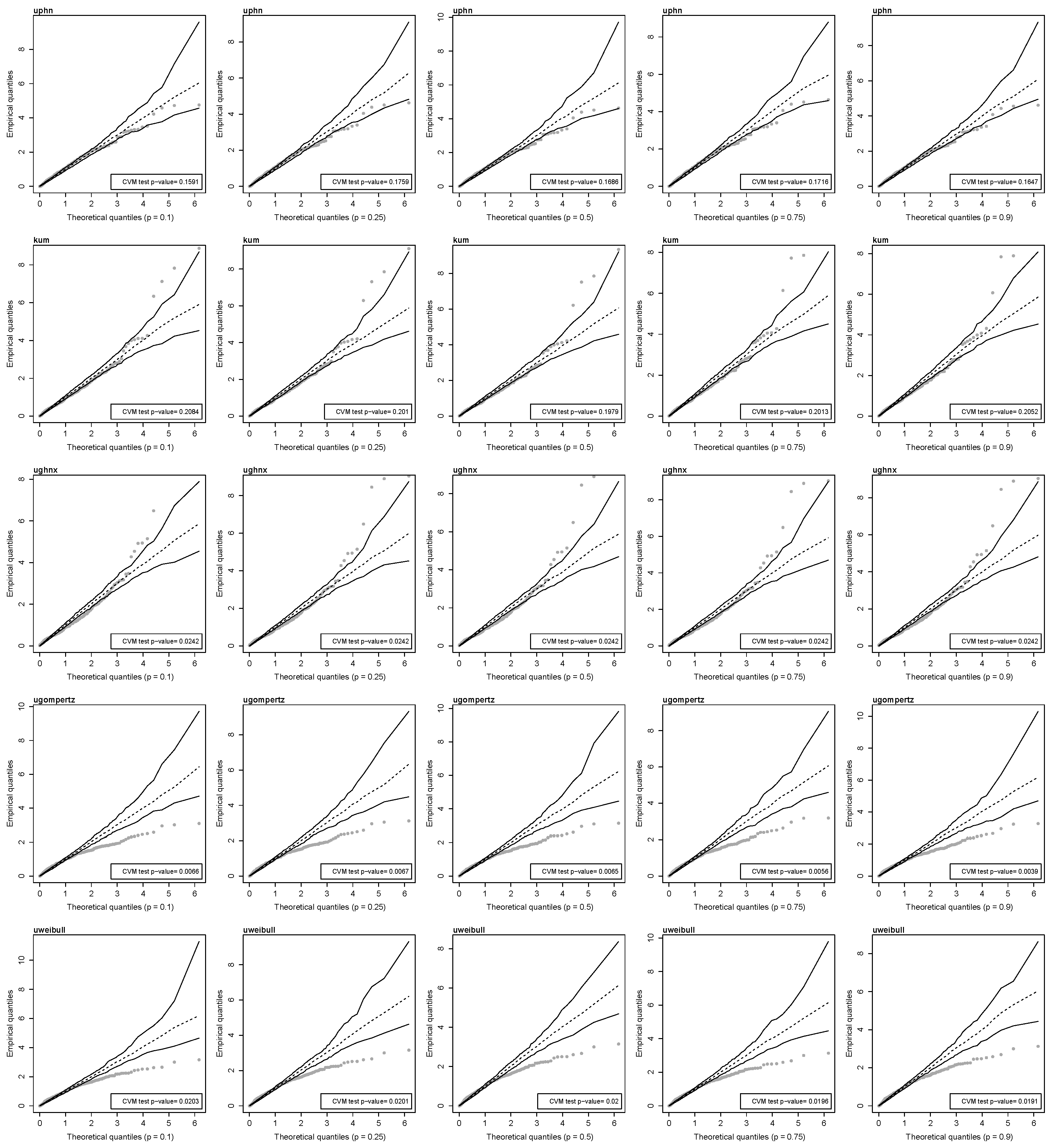
To validate these inferences, we conducted a diagnostic analysis for the fitted models. The Cox–Snell quantile residuals are considered, QQ plots are carried out by using their simulated envelopes. The Cramér–von Mises test is applied, where the null hypothesis is that the residuals come from an exponential distribution with a scale parameter of one. These plots are given in Figure 6. This figure suggests that the unit-power half-normal and Kumaraswamy quantile regression models provide a more substantial agreement with the data set compared to the unit-generalized half-normal-X, unit-Gompertz, and unit-Weibull quantile regression models, mainly because most of the residuals envelopes fail to cover the grey points, and the null hypothesis that the residuals come from an exponential distribution is rejected at the 5% significance level.

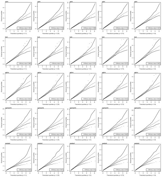
Figure 6. QQ plots with envelopes of Cox–Snell residuals for the indicated 100 p-th quantile level and Cramér-von Mises test p-value for residuals obtained from different distributions (uphn, kum, ughnx, ugompertz, and uweibull) with body fat data.

Therefore, the unit-power half-normal quantile regression model provides the best fit for the data, as it consistently shows the minimum goodness-of-fit measures, with all coefficients being statistically significant. The model’s assumptions are validated through diagnostic analyses, which confirm its reliability to describe the relationships between the covariates and arm fat percentage.

6.2. Application 2: Autologous Stem Cell Transplants Data Set

We consider another application linked to autologous peripheral blood stem cell (PBSC) transplants, which have been extensively utilized to accelerate hematologic recovery after myeloablative therapy for diverse malignant hematological disorders. The data set comprises a study involving 239 patients who agreed to undergo autologous PBSC transplant following myeloablative chemotherapy doses between 2003 and 2008 at the Edmonton Hematopoietic Stem Cell Lab within the Cross Cancer Institute of Alberta Health Services. This data set has been studied in [33] and contains information about the patients’ age, gender, and clinical characteristics. We aim to explain the response variable recovery rates for viable CD34+ cells (rcd) in terms of age, gender, and chemotherapy. The regression model assumed for ${\rho }_i$ is given by

$$\begin{array}{cc}\hfill logit\left({\rho }_i\left(p\right)\right)=& {\beta }_0\left(p\right)+{\beta }_1\left(p\right){\mathrm{Sexmale\_M}}_i+{\beta }_2\left(p\right){\mathrm{Age}}_i+{\beta }_3\left(p\right){\mathrm{Chemo}}_i,i=1,\dots ,239,\hfill \end{array}$$

(32)

where

$$\begin{array}{cc}\hfill {\mathrm{Sexmale\_M}}_i& =\left\{\begin{array}{cc}1,\hfill & \mathrm{if}\mathrm{the}\mathrm{gender}\mathrm{of}\mathrm{the}\mathrm{patient}i\mathrm{is}\mathrm{male}\hfill \\ 0,\hfill & \mathrm{if}\mathrm{the}\mathrm{gender}\mathrm{of}\mathrm{the}\mathrm{patient}i\mathrm{is}\mathrm{female}\hfill \end{array}\right.\hfill \end{array}$$

(33)

$$\begin{array}{cc}\hfill {\mathrm{Chemo}}_i& =\left\{\begin{array}{cc}1,\hfill & \mathrm{if}\mathrm{a}\mathrm{patient}i\mathrm{receives}\mathrm{a}\mathrm{chemotherapy}\mathrm{on}\mathrm{a}3-\mathrm{day}\mathrm{protocol}\hfill \\ 0,\hfill & \mathrm{if}\mathrm{a}\mathrm{patient}i\mathrm{receives}\mathrm{a}\mathrm{chemotherapy}\mathrm{on}\mathrm{a}1-\mathrm{day}\mathrm{protocol}.\hfill \end{array}\right.\hfill \end{array}$$

(34)

We examined the relationship between gender, age, chemotherapy, and the recovery rate for viable CD34+ cells by fitting the unit-power half-normal, the Kumaraswamy, the unit-generalized half-normal-X, the unit-Gompertz, and the unit-Birnbaum–Saunders quantile regression models, and evaluated the fits using goodness-of-fit measures.

Table 9 and Table 10 present the maximum likelihood estimates, their standard errors, and their p-values. For the unit-power half-normal and the unit-Gompertz quantile regression models, all quantile levels show statistically significant regression coefficients for the variables age and chemo at the 5% level. On the other hand, for the unit-generalized half-normal-X and the unit-Birnbaum–Saunders quantile regression models, the variable chemo is the only one statistically significant at the 5% level, while for the Kumaraswamy quantile regression, none of the three variables is statistically significant at the 5% level. Thus, based on the unit-power half-normal and the unit-Gompertz quantile regressions, we may conclude that the covariates Age and Chemo significantly affect the response variable recovery rate for viable CD34+ cells. Specifically, as Age increases, the recovery rate for viable CD34+ cells also increases. Additionally, patients receiving chemotherapy on a three-day protocol exhibit a higher recovery rate for viable CD34+ cells than those on a one-day protocol.

Table 9. Maximum likelihood estimates with their standard errors across different distributions (uphn, kum, ughnx, ugompertz, and ubs) with PBSC data.

p	Distribution	${\widehat{\mathit{\beta }}}_0$	$\mathit{SE}\left({\widehat{\mathit{\beta }}}_0\left(\mathit{p}\right)\right)$	${\widehat{\mathit{\beta }}}_1$	$\mathit{SE}\left({\widehat{\mathit{\beta }}}_1\left(\mathit{p}\right)\right)$	${\widehat{\mathit{\beta }}}_2$	$\mathit{SE}\left({\widehat{\mathit{\beta }}}_2\left(\mathit{p}\right)\right)$	${\widehat{\mathit{\beta }}}_3$	$\mathit{SE}\left({\widehat{\mathit{\beta }}}_3\left(\mathit{p}\right)\right)$	$\widehat{\mathit{\alpha }}$	$\mathit{SE}\left(\widehat{\mathit{\alpha }}\right)$	$\widehat{\mathit{\theta }}$	$\mathit{SE}\left(\widehat{\mathit{\theta }}\right)$
0.1	uphn	−0.498	0.211	0.097	0.090	0.015	0.003	0.397	0.094	1.284	0.104
	kum	0.281	0.156	0.023	0.055	0.003	0.002	0.085	0.065			6.707	0.454
	ughnx	−1.122	0.457	−0.152	0.167	0.001	0.007	0.380	0.192			0.645	0.028
	ugompertz	−0.456	0.231	0.094	0.098	0.014	0.004	0.337	0.106			2.789	0.342
	ubs	−0.150	0.350	−0.005	0.143	0.008	0.006	0.344	0.155			0.883	0.040
0.25	uphn	−0.180	0.210	0.097	0.090	0.015	0.003	0.397	0.094	1.285	0.104
	kum	0.653	0.191	0.029	0.071	0.004	0.003	0.113	0.085			6.708	0.454
	ughnx	0.320	0.422	−0.152	0.160	0.001	0.007	0.380	0.179			0.645	0.029
	ugompertz	−0.169	0.252	0.102	0.106	0.015	0.004	0.365	0.115			2.789	0.342
	ubs	0.491	0.314	−0.006	0.130	0.007	0.005	0.316	0.140			0.883	0.040
0.5	uphn	0.275	0.211	0.098	0.090	0.015	0.003	0.397	0.094	1.285	0.104
	kum	1.053	0.253	0.038	0.096	0.006	0.004	0.159	0.115			6.708	0.454
	ughnx	1.482	0.401	−0.152	0.158	0.001	0.006	0.38	0.174			0.645	0.029
	ugompertz	0.277	0.285	0.112	0.118	0.017	0.005	0.401	0.126			2.788	0.342
	ubs	1.179	0.291	−0.006	0.122	0.007	0.005	0.298	0.131			0.883	0.040
0.75	uphn	0.888	0.218	0.097	0.090	0.015	0.003	0.397	0.094	1.285	0.104
	kum	1.443	0.343	0.050	0.132	0.008	0.006	0.226	0.158			6.708	0.454
	ughnx	2.309	0.393	−0.152	0.157	0.001	0.006	0.380	0.172			0.645	0.029
	ugompertz	0.945	0.323	0.122	0.129	0.019	0.005	0.436	0.138			2.785	0.342
	ubs	1.820	0.282	−0.007	0.117	0.007	0.005	0.289	0.126			0.883	0.040
0.9	uphn	1.626	0.238	0.097	0.09	0.015	0.003	0.397	0.094	1.285	0.104
	kum	1.786	0.452	0.063	0.175	0.012	0.007	0.313	0.208			6.708	0.454
	ughnx	2.864	0.389	−0.152	0.157	0.001	0.006	0.380	0.171			0.645	0.029
	ugompertz	1.825	0.350	0.128	0.137	0.020	0.005	0.457	0.146			2.781	0.341
	ubs	2.338	0.279	−0.007	0.115	0.007	0.005	0.284	0.123			0.882	0.040

Table 10. p-values of Wald test for coefficients ${\beta }_j\left(p\right),j=0,1,2,3$, across different distributions (uphn, kum, ughnx, ugompertz, and ubs) for PBSC data.

p	Distribution			p-Value
		${\mathit{\beta }}_{\mathbf{0}}\left(\mathit{p}\right)$	${\mathit{\beta }}_{\mathbf{1}}\left(\mathit{p}\right)$	${\mathit{\beta }}_{\mathbf{2}}\left(\mathit{p}\right)$	${\mathit{\beta }}_{\mathbf{3}}\left(\mathit{p}\right)$
0.1	uphn	0.018	0.277	<${10}^{-3}$	<${10}^{-3}$
	kum	0.071	0.677	0.164	0.189
	ughnx	0.014	0.365	0.932	0.048
	ugompertz	0.048	0.338	<${10}^{-3}$	0.001
	ubs	0.669	0.974	0.165	0.027
0.25	uphn	0.392	0.277	<${10}^{-3}$	<${10}^{-3}$
	kum	<${10}^{-3}$	0.685	0.157	0.181
	ughnx	0.448	0.343	0.928	0.034
	ugompertz	0.502	0.338	<${10}^{-3}$	0.001
	ubs	0.118	0.965	0.156	0.024
0.5	uphn	0.193	0.276	<${10}^{-3}$	<${10}^{-3}$
	kum	<${10}^{-3}$	0.695	0.147	0.168
	ughnx	<${10}^{-3}$	0.337	0.926	0.028
	ugompertz	0.331	0.341	<${10}^{-3}$	0.001
	ubs	<${10}^{-3}$	0.958	0.15	0.023
0.75	uphn	<${10}^{-3}$	0.278	<${10}^{-3}$	<${10}^{-3}$
	kum	<${10}^{-3}$	0.706	0.134	0.151
	ughnx	<${10}^{-3}$	0.335	0.926	0.027
	ugompertz	0.003	0.346	<${10}^{-3}$	0.002
	ubs	<${10}^{-3}$	0.954	0.146	0.022
0.9	uphn	<${10}^{-3}$	0.277	<${10}^{-3}$	<${10}^{-3}$
	kum	<${10}^{-3}$	0.718	0.119	0.132
	ughnx	<${10}^{-3}$	0.335	0.925	0.026
	ugompertz	<${10}^{-3}$	0.350	<${10}^{-3}$	0.002
	ubs	<${10}^{-3}$	0.951	0.144	0.022

Table 11 displays the model selection criteria for the unit-power half-normal, the Kumaraswamy, the unit-generalized half-normal-X, the unit-Gompertz, and the unit-Birnbaum–Saunders quantile regressions. From this table, it can be said that the log-likelihood values of the unit-power half-normal quantile regression surpass those of the Kumaraswamy, the unit-generalized half-normal-X, the unit-Gompertz, and the unit-Birnbaum–Saunders quantile regressions. Therefore, based on these criteria, we may conclude that the unit-power half-normal model has a superior performance.

Table 11. Model selection criteria for different distributions (uphn, kum, ughnx, ugompertz, and ubs) for PBSC data.

p	Distribution	Neg2LogLike	AIC	BIC	HQIC
0.1	uphn	−384.643	−374.643	−357.26	−367.638
	kum	−384.207	−374.207	−356.824	−367.202
	ughnx	−190.055	−180.055	−162.673	−173.051
	ugompertz	−369.921	−359.921	−342.539	−352.916
	ubs	−313.824	−303.824	−286.442	−296.82
0.25	uphn	−384.643	−374.643	−357.26	−367.638
	kum	−384.234	−374.234	−356.851	−367.229
	ughnx	−190.055	−180.055	−162.673	−173.051
	ugompertz	−369.908	−359.908	−342.526	−352.904
	ubs	−313.861	−303.861	−286.479	−296.856
0.5	uphn	−384.643	−374.643	−357.26	−367.638
	kum	−384.271	−374.271	−356.889	−367.267
	ughnx	−190.055	−180.055	−162.673	−173.051
	ugompertz	−369.865	−359.865	−342.483	−352.861
	ubs	−313.889	−303.889	−286.507	−296.885
0.75	uphn	−384.643	−374.643	−357.26	−367.638
	kum	−384.318	−374.318	−356.936	−367.313
	ughnx	−190.055	−180.055	−162.673	−173.051
	ugompertz	−369.793	−359.793	−342.41	−352.788
	ubs	−313.906	−303.906	−286.524	−296.902
0.9	uphn	−384.643	−374.643	−357.26	−367.638
	kum	−384.367	−374.367	−356.985	−367.362
	ughnx	−190.055	−180.055	−162.673	−173.051
	ugompertz	−369.728	−359.728	−342.345	−352.723
	ubs	−313.915	−303.915	−286.532	−296.910

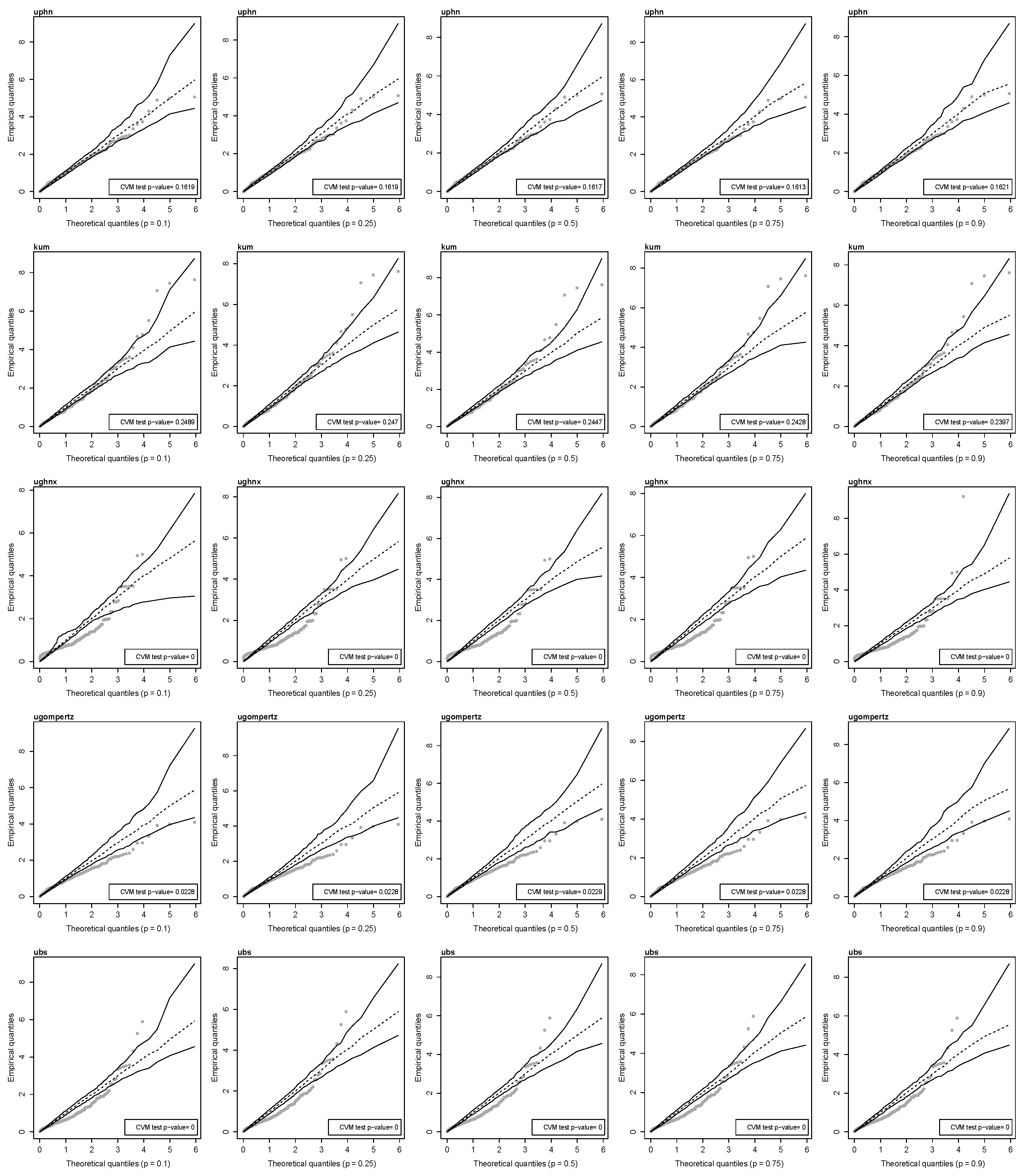
Finally, Figure 7 displays the QQ plots of the Cox–Snell quantile residuals and the p-value of the Cramér–von Mises test for the null hypothesis that the residuals come from an exponential distribution with a scale parameter of one. This figure indicates that most of the Cox–Snell quantile residuals obtained from the unit-power half-normal and the Kumaraswamy quantile regressions are inside the simulated envelopes. However, this is not the case for the Cox–Snell quantile residuals obtained from the unit-generalized half-normal-X, the unit-Gompertz, and the unit-Birnbaum–Saunders quantile regressions. These facts suggest that the assumption about Cox–Snell quantile residuals may not be right in those cases. This is validated by the p-value of the Cramér–von Mises test, where for the unit-generalized half-normal, the unit-Gompertz, and the unit-Birnbaum–Saunders quantile regressions, the p-value is less than 0.05, rejecting the null hypothesis that residuals come from an exponential distribution.

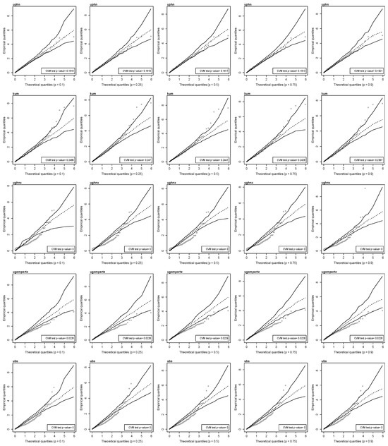
Figure 7. QQ plots with envelopes of Cox–Snell residuals for the proposed 100 p-th quantile level and Cramér–von Mises test p-value for residuals obtained from different distributions (uphn, kum, ughnx, ugompertz, and uweibull) with PBSC data.

Therefore, the unit-power half-normal quantile regression model is the best fit for the autologous stem cell transplants data. It consistently shows higher log-likelihood values and better model selection criteria compared to the other models. The significant coefficients for age and chemotherapy at the 5% level highlight their strong association with recovery rates for viable CD34+ cells. Furthermore, diagnostic analyses, including QQ plots and the Cramér–von Mises test, validate the model’s assumptions, confirming its superior performance.

7. Conclusions

In this paper, we have put forth a new quantile regression model. The predictor covariates were linked to the quantile of the dependent variable through the logit link function. We examined various aspects such as estimation, inference relying on the maximum likelihood method, and diagnoses via the quantile residual. We evaluated two real data sets drawn from medical data using our proposed quantile regression model and the previously introduced Kumaraswamy quantile regression models. The outcomes showed that our proposed quantile regression fitted well to the two real-world data sets. In the first one, the covariates age, body mass index, gender, and level of physical activity are statistically significant to evaluate the level of physical activity with the body fat in arms. For the second data set, the covariates age and chemo are statistically significant to explain the response variable recovery rates for viable CD34+ cells (rcd), using our proposed quantile regression model as an alternative to other rival models outlined in the related literature. We carried out a comparison based on different information criteria and the model’s goodness of fit, showing its suitability.

References

- Jones, M.C. Kumaraswamy’s Distribution: A Beta-Type Distribution with Some Tractability Advantages. Stat. Methodol. 2009, 6, 70–81. [Google Scholar] [CrossRef]
- Gómez-Déniz, E.; Sordo, M.A.; Calderín-Ojeda, E. The Log-Lindley distribution as an alternative to the beta regression model with applications in insurance. Insur. Math. Econ. 2014, 54, 49–57. [Google Scholar] [CrossRef]
- Mazucheli, J.; Bapat, S.R.; Menezes, A.F.B. A new one-parameter unit Lindley distribution. Chil. J. Stat. 2019, 1, 53–67. [Google Scholar]
- Abd El-Monsef, M.M.E.; El-Awady, M.M.; Seyam, M.M. A new quantile regression model for modelling child mortality. Int. J. Biomath. 2022, 10, 142–149. [Google Scholar]
- Altun, E.; Cordeiro, G.M. The unit-improved second-degree Lindley distribution: Inference and regression modelling. Comput. Stat. 2020, 35, 259–279. [Google Scholar] [CrossRef]
- Ahmad, H.H.; Almetwally, E.M.; Elgarhy, M.; Ramadan, D.A. On Unit Exponential Pareto Distribution for Modeling the Recovery Rate of COVID-19. Processes 2023, 11, 232. [Google Scholar] [CrossRef]
- Grassia, A. On a Family of Distributions with Argument between 0 and 1 Obtained by Transformation of the Gamma Distribution and Derived Compound Distributions. J. Stat. 1977, 19, 108–114. [Google Scholar] [CrossRef]
- Ghitany, M.; Mazucheli, J.; Menezes, A.; Alqallaf, F. The unit-inverse Gaussian distribution: A new alternative to two-parameter distributions on the unit interval. Commun. Stat. Theory Methods 2018, 48, 3423–3438. [Google Scholar] [CrossRef]
- Mazucheli, J.; Menezes, A.F.B.; Dey, S. The unit-Birnbaum-Saunders distribution with applications. Chil. J. Stat. 1977, 1, 47–57. [Google Scholar]
- Modi, K.; Gill, V. Unit Burr III distribution with application. J. Stat. Manag. Syst. 2019, 23, 579–592. [Google Scholar] [CrossRef]
- Korkmaz, M.; Chesneau, C. On the unit Burr-XII distribution with the quantile regression modeling and applications. Comput. Appl. Math. 2021, 40, 29. [Google Scholar] [CrossRef]
- Haq, M.; Hashmi, S.; Aidi, K.; Ramos, P.F.L. Unit Modified Burr-III Distribution: Estimation, Characterizations and Validation Test. Ann. Data Sci. 2023, 10, 415–449. [Google Scholar] [CrossRef]
- Bakouch, H.S.; Nikb, A.S.; Asgharzadehb, A.; Salinas, H.S. A flexible probability model for proportion data: Unit-half-normal distribution. Commun. Stat. Case Stud. Data Anal. 2021, 7, 271–288. [Google Scholar] [CrossRef]
- Gómez, Y.M.; Bolfarine, H. Likelihood-based inference for the power half-normal distribution. J. Stat. Theory Appl. 2015, 14, 383–398. [Google Scholar] [CrossRef]
- Barrios, L.; Gómez, Y.M.; Venegas, O.; Barranco-Chamorro, I.; Gómez, H.W. The Slashed Power Half-Normal Distribution with Applications. Mathematics 2022, 10, 1528. [Google Scholar] [CrossRef]
- Pallini, A. The discrete Powe Half-Normal Distribution. Statistica 2022, 82, 229–242. [Google Scholar]
- Lorenz, M.O. Methods of measuring the concentration of wealth. J. Am. Stat. Assoc. 1905, 9, 209–219. [Google Scholar] [CrossRef]
- Gini, C. On the measurement of concentration and variability of characters. Metron 2005, 1, 1–38. [Google Scholar]
- Gini, C. Measurement of inequality of incomes. Econ. J. 1921, 31, 124–126. [Google Scholar] [CrossRef]
- MacGillivray, H.L. Skewness and Asymmetry: Measures and Orderings. Ann. Stat. 1986, 14, 994–1011. [Google Scholar] [CrossRef]
- Moors, J.J. A quantile alternative for kurtosis. J. R. Stat. Soc. Ser. D 1988, 37, 25–32. [Google Scholar] [CrossRef]
- Balakrishnan, N.; Cohen, C.A. Order Statistics and Inference: Estimation Methods; Statistical Modeling and Decision Science; Elsevier Science: Amsterdam, The Netherlands, 1991. [Google Scholar]
- Bonferroni, C.E. Elementi di Statistica Generale; Libreria Seber: Firenze, Italy, 1930. [Google Scholar]
- Arcagni, A.; Porro, F. The Graphical Representation of Inequality. Rev. Colomb. Estad. 2014, 37, 419–436. [Google Scholar] [CrossRef]
- MacDonald, I.L. Does Newton-Raphson really fail? Stat. Methods Med Res. 2014, 23, 308–311. [Google Scholar] [CrossRef] [PubMed]
- R Core Team. R: A Language and Environment for Statistical Computing; R Foundation for Statistical Computing: Vienna, Austria, 2024; Available online: https://www.R-project.org/ (accessed on 31 July 2024).
- Cox, D.R.; Snell, E.J. A general definition of residuals. J. Royal Stat. Soc. Ser. B 1968, 30, 248–265. [Google Scholar] [CrossRef]
- Bolar, K. STAT: Interactive Document for Working with Basic Statistical Analysis. 2019. Available online: https://cran.r-project.org/web/packages/STAT/index.html (accessed on 1 April 2024).
- Mazucheli, J.; Menezes, A.F.; Dey, S. Unit-Gompertz Distribution with Applications. Statistica 2019, 79, 25–43. [Google Scholar]
- Mazucheli, J.; Menezes, A.F.B.; Alqallaf, F.; Ghitany, M.E. Bias-Corrected Maximum Likelihood Estimators of the Parameters of the Unit-Weibull Distribution. Austrian J. Stat. 2021, 50, 41–53. [Google Scholar]
- Menezes, A.F.B. unitquantreg: Parametric Quantile Regression Models for Bounded Data. 2023. Available online: https://cran.r-project.org/web/packages/unitquantreg/index.html (accessed on 15 April 2024).
- Petterle, R.; Bonat, W.; Scarpin, C.; Jonasson, T.; Borba, V. Multivariate quasi-beta regression models for continuous bounded data. Int. J. Biostat. 2021, 17, 39–53. [Google Scholar] [CrossRef]
- Yang, H.; Acker, J.P.; Cabuhat, M.; Letcher, B.; Larratt, L.; McGann, L.E. Association of post-thaw viable CD34+ cells and CFU-GM with time to hematopoietic engraftment. Bone Marrow Transplant. 2005, 35, 881–887. [Google Scholar] [CrossRef]
Disclaimer/Publisher’s Note: The statements, opinions and data contained in all publications are solely those of the individual author(s) and contributor(s) and not of MDPI and/or the editor(s). MDPI and/or the editor(s) disclaim responsibility for any injury to people or property resulting from any ideas, methods, instructions or products referred to in the content. |
© 2024 by the authors. Licensee MDPI, Basel, Switzerland. This article is an open access article distributed under the terms and conditions of the Creative Commons Attribution (CC BY) license (https://creativecommons.org/licenses/by/4.0/).