Numerical Computation of 2D Domain Integrals in Boundary Element Method by (α, β) Distance Transformation for Transient Heat Conduction Problems

Abstract

When the time-dependent boundary element method, also termed the pseudo-initial condition method, is employed for solving transient heat conduction problems, the numerical evaluation of domain integrals is necessitated. Consequently, the accurate calculation of the domain integrals is of crucial importance for analyzing transient heat conduction. However, as the time step decreases progressively and approaches zero, the integrand of the domain integrals is close to singular, resulting in large errors when employing standard Gaussian quadrature directly. To solve the problem and further improve the calculation accuracy of the domain integrals, an (α, β) distance transformation is presented. Distance transformation is a simple and efficient method for eliminating near-singularity, typically applied to nearly singular integrals. Firstly, the (α, β) coordinate transformation is introduced. Then, a new distance transformation for the domain integrals is constructed by replacing the shortest distance with the time step. With the new method, the integrand of the domain integrals is substantially smoothed, and the singularity arising from small time steps in the domain integrals is effectively eliminated. Thus, more accurate results can be obtained by the (α, β) distance transformation. Different sizes of time steps, positions of source point, and shapes of integration elements are considered in numerical examples. Comparative studies of the numerical results for the domain integrals using various methods demonstrate that higher accuracy and efficiency are achieved by the proposed method.

1. Introduction

Numerical methods are extensively employed across various engineering applications [1,2,3]. In many practical engineering scenarios, the problems are transient, which means that they are space- and time-dependent. Since it is usually very difficult to find an analytical solution, numerical methods are widely employed for these problems, such as the finite element method (FEM) [4], the finite difference method (FDM) [5,6,7], and the boundary element method (BEM) [8,9,10]. Compared to other methods, the BEM is identified as being a significantly simpler and more efficient tool for solving transient heat conduction problems. Yu et al. [11,12,13] introduced the isogeometric dual reciprocity boundary element method to solve the problems of transient heat conduction. Erhart et al. [14] adopted a parallel domain decomposition boundary element method approach to solve large-scale transient heat conduction problems. Feng et al. [15,16] proposed an analytically integrated radial integration BEM and a meshless interface integral BEM for solving transient heat conduction. Zhang et al. [17,18] developed the boundary face method for analyzing transient heat conduction.

In the analysis of transient heat conduction, the pseudo-initial method, based on the time-dependent fundamental solution, is prevalently employed within the BEM. The method employs the temperature calculated in the previous step as the initial condition for the current step, necessitating careful consideration of the domain integral associated with this pseudo-initial condition. Although the domain integrals typically exhibit regularity, the integrand (time-dependent fundamental solution) of these integrals may vary dramatically near the source point as the time step approaches zero, with the domain integrals exhibiting properties similar to singular integrals. The numerical integration of functions possessing the above characteristics leads to numerical instability in the BEM solution, as evidenced in references [19,20,21]. Such conditions render the Gaussian quadrature method inadequate for achieving accurate calculations. Therefore, eliminating the singularity caused by the time step is essential for accurately computing domain integrals, which is crucial for solving transient heat conduction problems using the pseudo-initial condition method.

Various strategies have been developed to counteract the adverse effects arising from the use of small time steps. Dong et al. [22,23] introduced a method combining a coordinate transformation with an element subdivision technique. However, this technique is time-consuming and requires more complex coding due to the need to divide the integration element into enough sub-elements. Gao et al. [24,25,26] proposed the radial integration method, which converted the domain integrals into equivalent boundary integrals, but its efficiency is compromised in large-scale problem applications. In recent work, Dong et al. expanded upon the sinh transformation [27] and the distance transformation [28], originally applied to the nearly singular integrals [29,30,31,32,33,34], to calculate the domain integrals. These transformations are implemented based on the polar coordinate transformation.

To improve calculation accuracy and simplify the implementation process, an (α, β) distance transformation is proposed to compute the 2D domain integrals in the BEM for transient heat conduction problems. The (α, β) coordinate transformation is initially introduced to smooth the integrand to some degree. The shortest distance in the nearly singular integral is replaced by the time step, and the new distance transformation is constructed in the α direction. In this paper, a new distance transformation is represented and combined with the (α, β) coordinate transformation. The singularity arising from small time steps in the domain integral is effectively eliminated by the Jacobian of the (α, β) distance transformation. Comparative analyses of the numerical examples demonstrated that the proposed method is simpler and more effective than the other four existing methods. Thus, the new method can be effectively applied to accurately compute the 2D domain integrals.

The structure of the paper is organized as follows. The boundary integral equation, the domain integral, and the element subdivision technique are discussed in Section 2. The implementation of the proposed method is detailed in Section 3. Several numerical examples are given to demonstrate the validity of the method in Section 4. The conclusion is provided in Section 5.

2. General Description

2.1. Boundary Integral Equation

Assuming the material is isotropic, the governing equation for transient heat conduction problems without heat sources is initially given as follows:

$${\nabla }^{2}u\left(\mathbf{X},t\right)-{\displaystyle \frac{1}{k}}{\displaystyle \frac{\partial u\left(\mathbf{X},t\right)}{\partial t}}=0,$$

(1)

where u (X, t) denotes the temperature in the coordinate X at the time t; and k is the diffusion coefficient.

The boundary integral equation [2,3] for transient heat conduction in an isotropic, homogeneous medium Ω bounded by Γ can be expressed as follows:

$$\begin{gathered} c\left(\mathbf{Y}\right)u\left(\mathbf{Y},t_F\right)+k{\displaystyle {\int }_{t_0}^{t_F}{\displaystyle {\int }_{\Gamma }u\left(\mathbf{X},t\right)}}{q}^{*}\left(\mathbf{Y},\mathbf{X},t_F,t\right)d\Gamma \left(\mathbf{X}\right)dt \\ =k{\displaystyle {\int }_{t_0}^{t_F}{\displaystyle {\int }_{\Gamma }q}}\left(\mathbf{X},t\right)u^{*}\left(\mathbf{Y},\mathbf{X},t_F,t\right)d\Gamma \left(\mathbf{X}\right)dt \\ +{\displaystyle {\int }_{\Omega }{u}_0}\left(\mathbf{X},t_0\right)u^{*}\left(\mathbf{Y},\mathbf{X},t_F,t_0\right)d\Omega \left(\mathbf{X}\right), \end{gathered}$$

(2)

where Y and X denote the source point and the field point, respectively. c(Y) is an internal angle function that varies according to the geometrical shape of the boundary at Y. u₀(X, t₀) is the initial temperature. t₀ and t_F represent the initial time and the end time of the time step, respectively. u* and q* denote the time-dependent fundamental solution and the normal derivative of u*, respectively.

The time-dependent fundamental solution u* [2,3] can be expressed as follows:

$$u^{*}={\displaystyle \frac{1}{4\pi k\tau }}\exp \left(-{\displaystyle \frac{r^2}{4k\tau }}\right),$$

(3)

where τ = t_F − t₀, which is the time step. The distance between the source Y and the field point X is denoted by r.

2.2. Domain Integral

The domain integral [22,23,28,29] of the boundary integral equation is obtained as follows:

$$I={\displaystyle {\int }_{\Omega }{u}_0}\left(\mathbf{X},t_0\right)u^{*}\left(\mathbf{Y},\mathbf{X},t_F,t_0\right)d\Omega \left(\mathbf{X}\right)={\displaystyle {\int }_{\Omega }\frac{u_0\left(\mathbf{X},t_0\right)}{4\pi k\tau }\exp \left(-\frac{r^2}{4k\tau }\right)d\Omega \left(\mathbf{X}\right)},$$

(4)

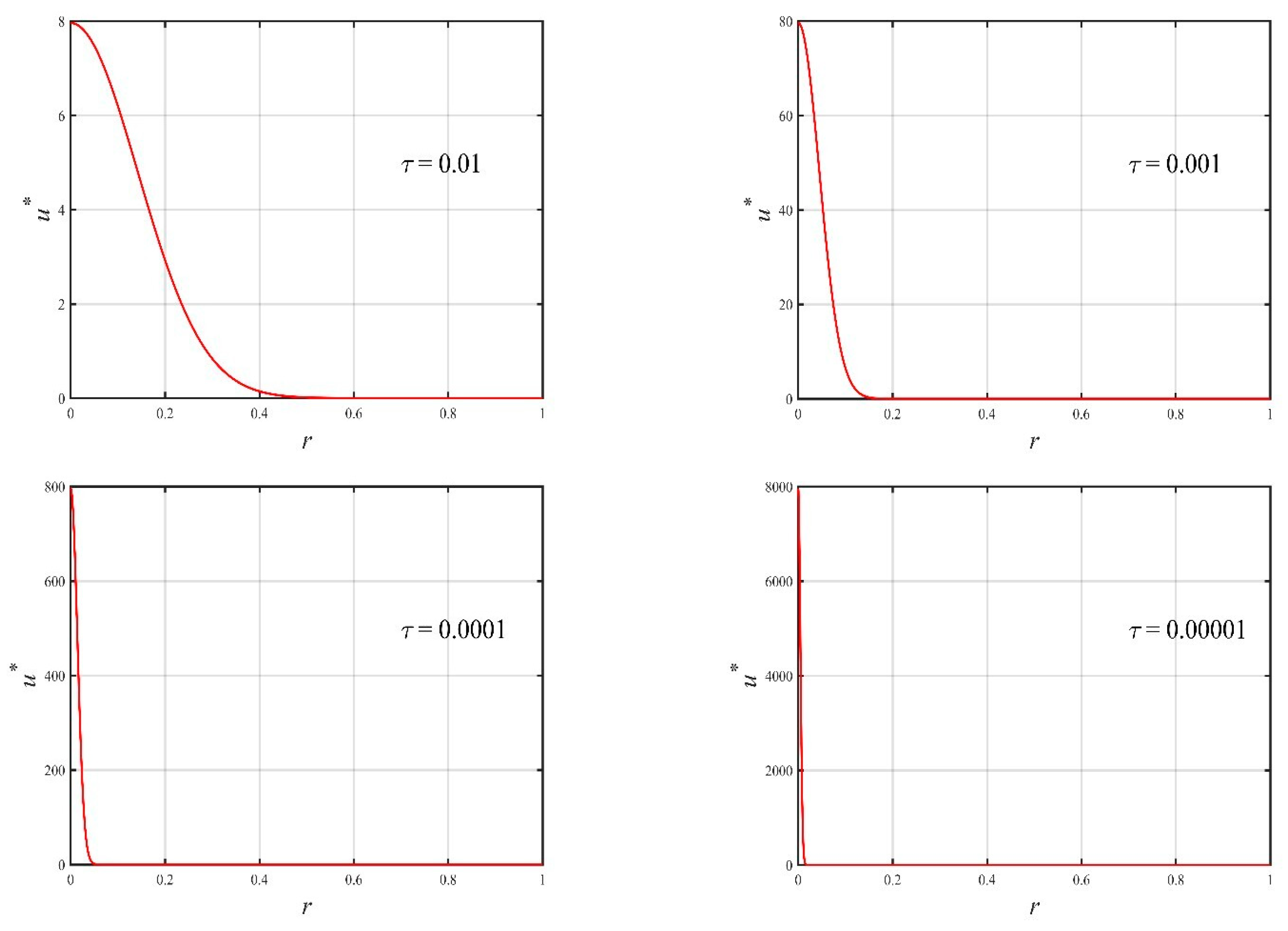
where u₀(X, t₀) is a regular function that can be calculated exactly by standard Gaussian quadrature. The influence of the time step size on the integral is evident from (4). As the time step τ approaches zero, the integrand tends to infinity, which consequently undermines the accuracy of calculating the integral I using standard Gaussian quadrature [22,23,29]. The variation of u* with respect to r for different time steps is depicted in Figure 1.

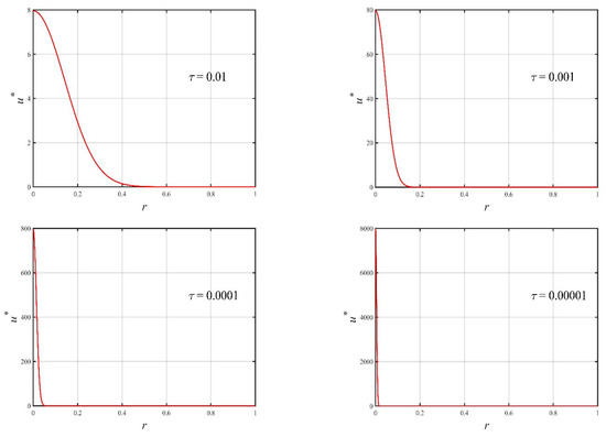
Figure 1. Variation of u* with respect to r for different time steps τ.

2.3. The Subdivision of the Integration Element

To improve the calculation accuracy of the domain integral, the subdivision of the quadrilateral integration element is employed prior to applying the proposed method, as depicted in Figure 2. Based on the position of the source point (x₀, y₀) on the quadrilateral, the integration element is subdivided into different numbers of sub-triangles by connecting the source to the vertices of the element, as illustrated in Figure 2a–c.

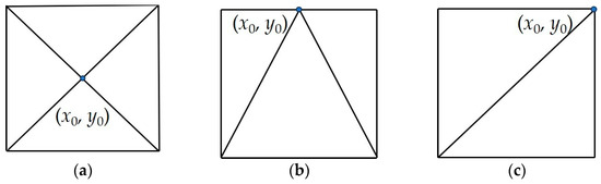
Figure 2. Subdivision of the integration element when the source point lies (a) inside the quadrilateral, (b) on an edge, or (c) on a vertex, respectively.

3. (α, β) Distance Transformation

In this section, the (α, β) coordinate transformation is first introduced. Then, to eliminate the adverse effect arising from the small time step in the calculation of the domain integrals, a new distance transformation is constructed.

3.1. The (α, β) Coordinate Transformation

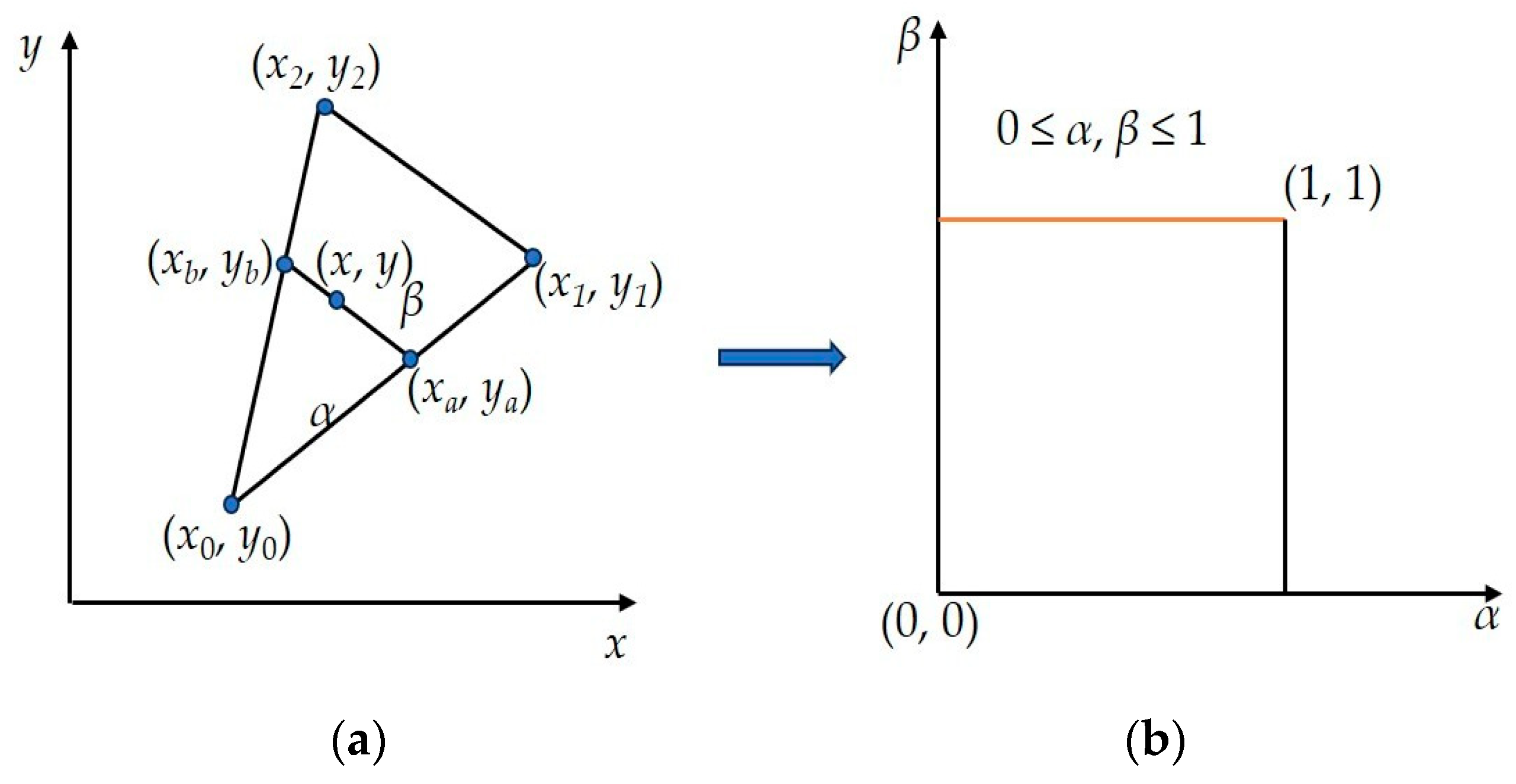
In this section, the (α, β) transformation proposed by Zhang et al. [35], akin to the polar coordinate transformation, is initially introduced. As illustrated in Figure 3, the sub-triangular element is mapped to a unit quadrilateral using the (α, β) transformation, wherein the source point (x₀, y₀) corresponds to the line where β = 1.

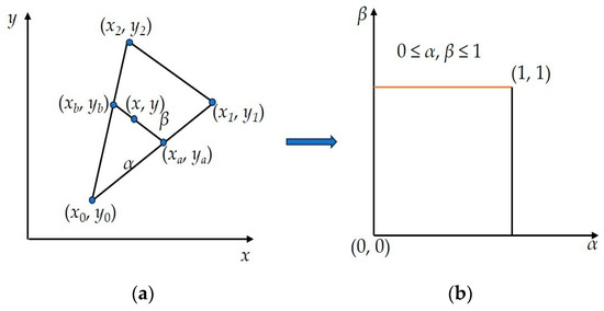
Figure 3. (α, β) transformation: (a) arbitrary sub-triangle in (x, y) coordinate system; (b) mapping the sub-triangle into a unit square in the (α, β) coordinate system.

To implement the mapping depicted in Figure 3, the following expressions can be employed:

$$\left\{\begin{array}{l}{x}_a=x_0+\left(x_1-x_0\right)\alpha \\ y_a=y_0+\left(y_1-y_0\right)\alpha \end{array}\right.$$

(5)

$$\left\{\begin{array}{l}{x}_b=x_0+\left(x_2-x_0\right)\alpha \\ y_b=y_0+\left(y_2-y_0\right)\alpha \end{array}\right.$$

(6)

$$\left\{\begin{array}{l}x=x_a+\left(x_b-x_a\right)\beta \\ y=y_a+\left(y_b-y_a\right)\beta \end{array}\right.,$$

(7)

where α and β are the two variables representing the proportions.

Combining (5)–(7), the coordinate of the arbitrary point (x, y) on the integration element can be obtained.

$$\left\{\begin{array}{l}x=x_0+\left(x_1-x_0\right)\alpha +\left(x_2-x_1\right)\alpha \beta \\ y=y_0+\left(y_1-y_0\right)\alpha +\left(y_2-y_1\right)\alpha \beta \end{array}\right..$$

(8)

Given that the initial temperature in (4), u₀(X, t₀), is a regular function, for simplicity, it is assumed to be 1 in this paper. Consequently, under the influence of the (α, β) transformation, (4) is written as follows:

$$I={\displaystyle {\int }_0^1{\displaystyle {\int }_0^1\frac{1}{4\pi k\tau }\exp \left(-\frac{r^2\left(\alpha ,\beta \right)}{4k\tau }\right)2\alpha S}}d\alpha d\beta ,$$

(9)

where the term 2αS is the Jacobian in the transformation from the (x, y) coordinate system to the (α, β) coordinate system and S is the area of the sub-triangular element. According to (9), the variables α and β in the (α, β) coordinate system are constrained to the interval [0, 1]. This constraint simplifies and facilitates the integral calculation. Additionally, the Jacobian of the transformation can enhance the smoothness of the integrand, thereby improving the accuracy of the domain integral.

3.2. New Distance Transformation

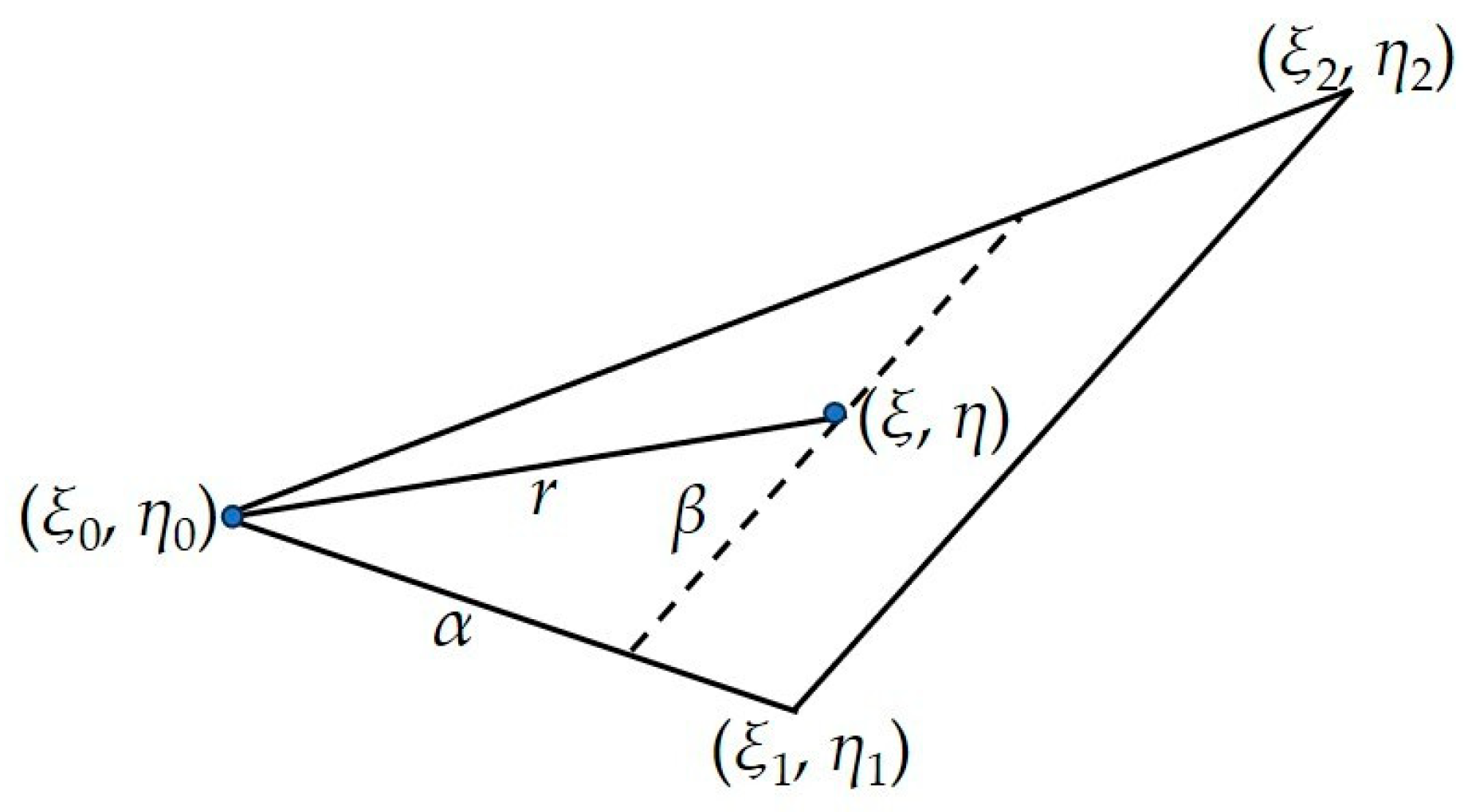
As shown in Figure 4, the distance between the source point and the field point is obtained by applying the Taylor expansion near the source point and the (α, β) transformation (Equation (8)).

$$\begin{gathered} x_k-y_k={\displaystyle \frac{\partial x_k}{\partial \xi }}{|}_{\begin{array}{l}\xi ={\xi }_0\\ \eta ={\eta }_0\end{array}}\left(\xi -{\xi }_0\right)+{\displaystyle \frac{\partial x_k}{\partial \eta }}{|}_{\begin{array}{l}\xi ={\xi }_0\\ \eta ={\eta }_0\end{array}}\left(\eta -{\eta }_0\right)+o\left({\left(\xi -{\xi }_0\right)}^2+{\left(\eta -{\eta }_0\right)}^2\right) \\ =\alpha A_k\left(\beta \right)+o\left({\alpha }^2\right),\hspace{1em}\hspace{1em}\hspace{1em}\hspace{1em}\hspace{1em}\hspace{1em}\hspace{1em}\hspace{1em}\hspace{1em}\hspace{1em}\hspace{1em}\hspace{1em}\hspace{1em}\hspace{1em}\hspace{1em}\hspace{1em}\hspace{1em}\hspace{1em}\hspace{1em}\hspace{1em}\hspace{1em} \end{gathered}$$

(10)

where x_k,k=1,2 and y_k,_k=1,2 represent the nodal coordinates of the field point and the source point, respectively. (ξ, η) and (ξ₀, η₀) denote the parametric coordinates of the field point X and the source point Y. The term $A_k(\beta )$ is ${\displaystyle \frac{\partial x_k}{\partial \xi }}{|}_{\begin{array}{l}\xi ={\xi }_0\\ \eta ={\eta }_0\end{array}}[({\xi }_1-{\xi }_0)+({\xi }_2-{\xi }_1)\beta ]$$+{\displaystyle \frac{\partial x_k}{\partial \eta }}{|}_{\begin{array}{l}\xi ={\xi }_0\\ \eta ={\eta }_0\end{array}}[({\eta }_1-{\eta }_0)+({\eta }_2-{\eta }_1)\beta ]$. The coordinates (ξ₁, η₁) and (ξ₂, η₂) correspond to the other vertices of the sub-triangle in the parametric space.

Figure 4. The distance between the source point and the field point in local space.

The square of the distance between the source point and the field point can be expressed as follows:

$$r^2=\left(x_k-y_k\right)\left(x_k-y_k\right)={\alpha }^{2}A\left(\beta \right)+o\left({\alpha }^3\right),$$

(11)

where $A\left(\beta \right)=\sqrt{A_k\left(\beta \right)A_k\left(\beta \right)}$.

When the time step involved in the integrand is very small, the numerical calculation of the domain integral is negatively impacted. To eliminate these effects, a new distance transformation is proposed that utilizes the time step as the shortest distance in the nearly singular integral.

$$\left\{\begin{array}{l}v\left(\alpha ,\beta \right)=\log \sqrt{{\alpha }^2+{\left({\displaystyle \frac{\sqrt{\tau }}{A_k\left(\beta \right)}}\right)}^2}\\ \alpha \left(v\right)=\sqrt{\exp \left(2v\right)-{\left({\displaystyle \frac{\sqrt{\tau }}{A_k\left(\beta \right)}}\right)}^2}\end{array}\right..$$

(12)

From (12), the Jacobian of the distance transformation can be obtained as follows:

$$J={\displaystyle \frac{d\alpha }{dv}}={\displaystyle \frac{\exp \left(2v\right)}{\sqrt{\exp \left(2v\right)-{\left(\frac{\sqrt{\tau }}{A_k\left(\beta \right)}\right)}^2}}}.$$

(13)

Based on (12) and (13), the integral in (9) can be transformed into the following:

$$\begin{gathered} I={\displaystyle {\int }_0^1{\displaystyle {\int }_0^1\frac{1}{4\pi k\tau }\exp \left(-\frac{r^2\left(\alpha ,\beta \right)}{4k\tau }\right)2\alpha S}}d\alpha d\beta \\ \hspace{1em}\hspace{1em}\hspace{1em}\hspace{1em}\hspace{1em}\hspace{1em}={\displaystyle {\int }_0^1{\displaystyle {\int }_{\log \frac{\sqrt{\tau }}{A_k\left(\beta \right)}}^{\sqrt{1+{\left(\frac{\sqrt{\tau }}{A_k\left(\beta \right)}\right)}^2}}\frac{1}{4\pi k\tau }\exp \left(-\frac{r^2\left(v,\beta \right)}{4k\tau }\right)\exp \left(2v\right)2S}}dvd\beta \end{gathered}$$

(14)

In Equation (12), $\alpha \left(v\right)=\sqrt{\exp \left(2v\right)-{\left(\sqrt{\tau }/A_k\left(\beta \right)\right)}^2}$ is provided. From (14), it can be observed that the term exp(2v) includes the time step τ, which can effectively eliminate the time step in the denominator of the integrand. As a result, the adverse effects of the small time step on the integral calculation are significantly eliminated.

4. Numerical Examples

In this section, numerical examples are presented to validate the proposed method. The following domain integral is considered:

$$I={\displaystyle {\int }_{\Omega }\frac{1}{4\pi k\tau }\exp \left(-\frac{r^2}{4k\tau }\right)}d\Omega ,$$

(15)

where the diffusion coefficient k is assumed to be 1 in all examples.

The calculation accuracy and stability of all methods are compared using the following definition of relative error:

$$\mathrm{Relative} \mathrm{Error}=\left|{\displaystyle \frac{I_{numerical}-I_{exact}}{I_{numerical}}}\right|,$$

(16)

where I_numerical and I_exact are the numerical solutions obtained by various methods of the considered integral and the exact solution, respectively. The exact solution is obtained by the element subdivision method [36] with enough sub-elements, which is considered stable and inefficient.

4.1. Example 1

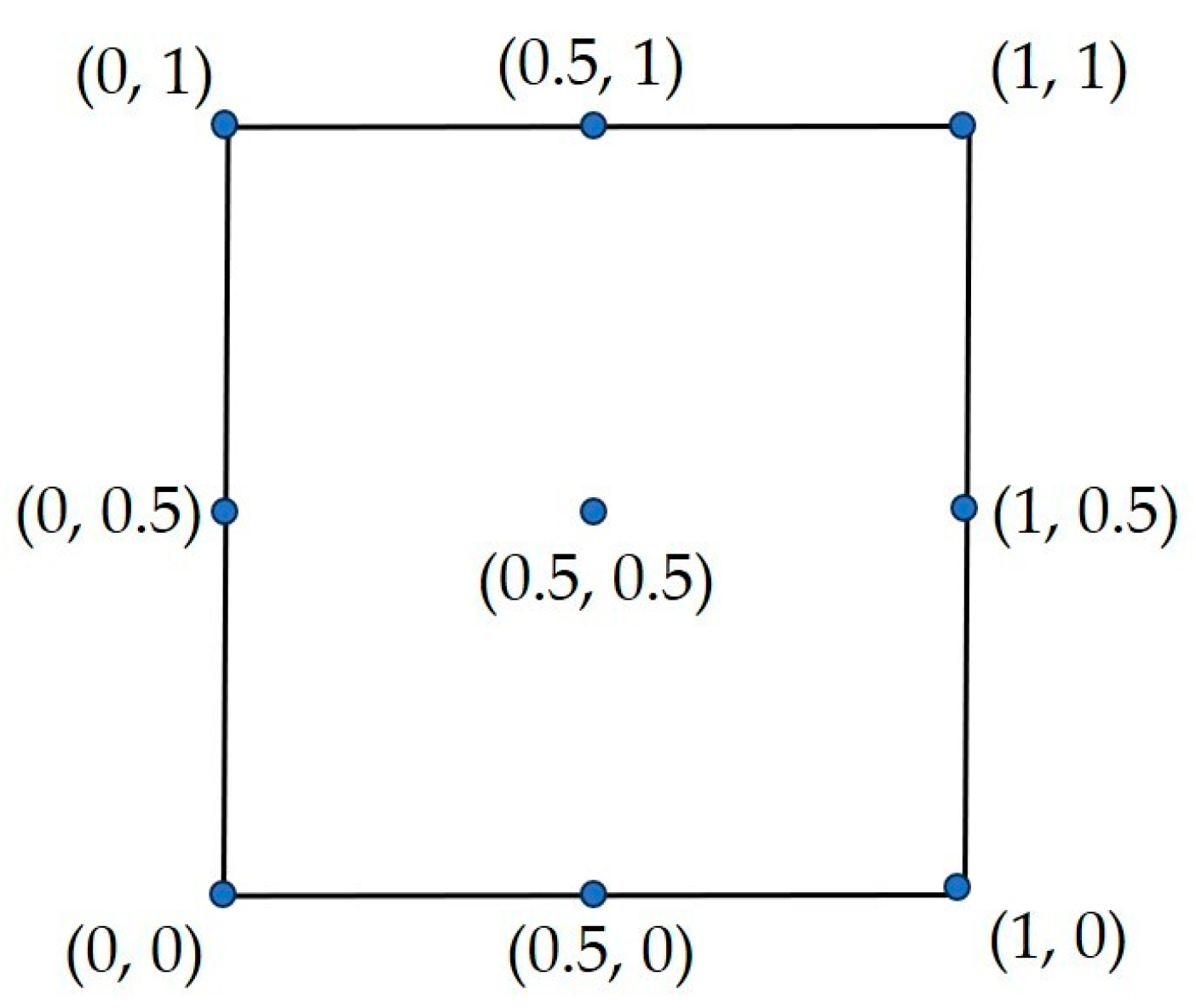
With different time step sizes and Gaussian points, the impact on Gaussian quadrature is considered in this example. The integration element, as shown in Figure 5, with vertex coordinates (1, 1), (0, 1), (0, 0), and (1, 0), is used. The relative errors for the domain integral in (15) are illustrated in Table 1. τ is the size of the time step. The equation 5 × 5 denotes the Gaussian points used in Gaussian quadrature.

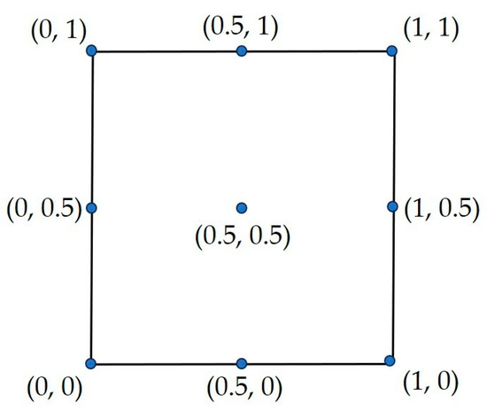
Figure 5. Nodal coordinates of the quadrilateral element.

Table 1. Relative errors of Gaussian quadrature for the domain integral in (15), with different numbers of Gaussian points. Errors greater than 1 are indicated as E.

τ	τ = 0.1	τ = 0.01	τ = 0.001	τ = 0.0001	τ = 0.00001
5 × 5	2.132 × 10−6	5.524 × 10−2	E	E	E
10 × 10	5.732 × 10−15	1.299 × 10−5	5.647 × 10−1	E	E
15 × 15	4.504 × 10−15	3.032 × 10−10	9.135 × 10−2	E	E
20 × 20	3.275 × 10−15	1.667 × 10−15	5.677 × 10−3	E	E
25 × 25	2.456 × 10−15	3.789 × 10−14	1.852 × 10−4	E	E
30 × 30	4.913 × 10−15	6.667 × 10−16	3.245 × 10−6	6.931 × 10−1	E
35 × 35	1.024 × 10−15	1.245 × 10−14	3.208 × 10−8	6.052 × 10−1	E
40 × 40	2.047 × 10−15	6.333 × 10−14	1.867 × 10−10	2.691 × 10−1	E
45 × 45	6.346 × 10−15	2.867 × 10−14	1.290 × 10−12	1.515 × 10−1	E
50 × 50	8.188 × 10−16	3.356 × 10−14	7.352 × 10−13	6.680 × 10−2	E

As shown in Table 1, even with the smaller number of Gaussian points, employing direct Gaussian quadrature can yield accurate results when the time step is large. However, when the time step is progressively decreased to less than 0.001, despite employing a large number of Gaussian points, the Gaussian quadrature method proves inadequate for accurate results.

4.2. Example 2

This example examines the situation where the source point is located at the center of the quadrilateral element, illustrating the impact of the time step on various methods. The integration element in Figure 5 is used. Relative errors for the domain integral in (15), calculated using various methods across different time step sizes, are listed in Table 2. ‘Direct’ denotes the direct Gaussian quadrature method. ‘Polar’ is the polar coordinate transformation. ‘Sinh’ and ‘Distance’ represent the sinh transformation and the distance transformation based on the (ρ, θ) coordinate system, respectively. The (α, β) distance transformation, our suggested method, is indicated by ‘αβDistance’. The 20 × 20 Gaussian points are used in all methods.

Table 2. Relative errors of various methods for the domain integral in Equation (15), with different time steps τ. Errors greater than 1 are indicated as E.

(0.5, 0.5)	τ = 0.1	τ = 0.01	τ = 0.001	τ = 0.0001	τ = 0.00001
Direct	3.275 × 10−15	1.667 × 10−15	5.677 × 10−3	E	E
Polar	6.755 × 10−15	4.333 × 10−15	3.238 × 10−9	2.253 × 10−4	1.078 × 10−1
Sinh	7.574 × 10−15	1.645 × 10−14	1.331 × 10−8	1.559 × 10−5	1.042 × 10−5
Distance	9.007 × 10−15	8.667 × 10−15	1.258 × 10−9	1.908 × 10−6	1.780 × 10−6
αβDistance	7.984 × 10−15	1.045 × 10−14	1.614 × 10−13	1.911 × 10−9	2.304 × 10−7

Table 2 demonstrates that all methods maintain high accuracy when the values of τ are large; however, significant errors are incurred with the use of direct Gaussian quadrature as the time step decreases. Superior accuracy and stability are consistently exhibited by the proposed method when compared to other methods.

4.3. Example 3

In this example, the (α, β) distance transformation is compared with the element subdivision technique incorporating the (α, β) coordinate transformation as described in reference [22]. The integration element, depicted in Figure 5, is utilized with the coordinate of the source point set to (0.5, 0.5). The relative errors of the two methods used for the domain integral calculation in Equation (15), as well as the computation time for 10000 iterations, are presented in Table 3 and Table 4, respectively. ‘(α, β)’ denotes the technique from reference [22] that is utilized. In this method, 20 × 20 Gaussian integration points are used for the subdivided sub-triangles, and 10 × 10 Gaussian integration points are employed for the subdivided sub-quadrilaterals. ‘αβDistance’ indicates the (α, β) distance transformation, our suggested method, where 20 × 20 Gaussian integration points are utilized for each of the four sub-triangles. Consequently, a smaller number of Gaussian points are employed by the proposed method.

Table 3. Relative errors for the domain integral in Equation (15) using the method in reference [22] and the (α, β) distance transformation.

(0.5, 0.5)	τ = 0.1	τ = 0.01	τ = 0.001	τ = 0.0001	τ = 0.00001
(α, β)	1.842 × 10−15	4.222 × 10−15	1.103 × 10−10	1.248 × 10−8	3.074× 10−8
αβDistance	7.984 × 10−15	1.045 × 10−14	1.614 × 10−13	1.911 × 10−9	2.304 × 10−7

Table 4. Computation time for the domain integral in Equation (15) using the technique in reference [22] and the (α, β) distance transformation running 10,000 times.

(0.5, 0.5)	τ = 0.1	τ = 0.01	τ = 0.001	τ = 0.0001	τ = 0.00001
(α, β)	25,775 ms	25,788 ms	35,453 ms	36,264 ms	36,586 ms
αβDistance	7420 ms	7523 ms	7336 ms	7684 ms	7643 ms

From the comparison in Table 3 and Table 4, the following conclusions can be drawn: The proposed method achieves similar accuracy to that of the method in reference [22] while requiring fewer Gaussian integration points. Additionally, significantly less time is consumed by the new method compared to the ‘(α, β)’ method for calculating the domain integral. The above results derived from the element subdivision method are attributed to the requirement of dividing the integration element into enough sub-elements, a process that is time-consuming and necessitates more complex code. However, the proposed method needs only the subdivision of the integration element by connecting the source point with the vertices of the element and employing the new distance transformation to eliminate the singularity in the domain integral. Thus, it can be concluded that the (α, β) distance transformation demonstrates higher efficiency.

4.4. Example 4

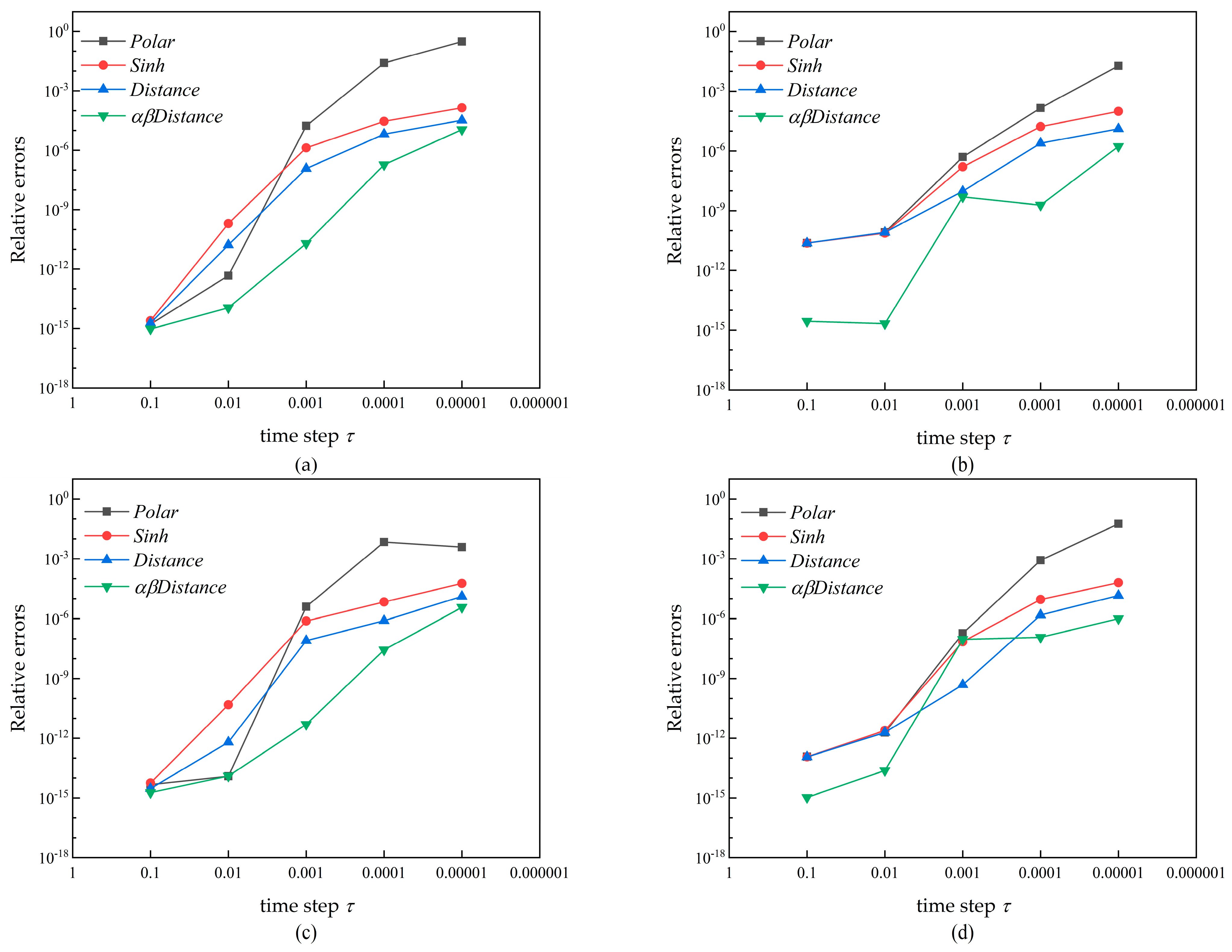
The effect of different source point locations on numerical calculations is considered in this example. To demonstrate the superior results achievable with the proposed method at different source points, particular attention is given to situations where the source point coincides with a vertex, is located on an edge of the integration element, or is close to a vertex or an edge, as depicted in Figure 6a–d. The results calculated by the various methods for the domain integral are presented in Table 5. In Figure 7a–d, the results of various methods at different source point positions are shown. ‘Polar’ denotes the polar coordinate transformation. ‘Sinh’ and ‘Distance’ refer to the sinh transformation and the new distance transformation, respectively. ‘αβDistance’ indicates the (α, β) distance method. The 20 × 20 Gaussian points are used in all methods.

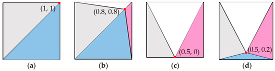
Figure 6. The subdivision of the quadrilateral element when the source point is located at (a) (1, 1), (b) (0.8, 0.8), (c) (0.5, 0), and (d) (0.5, 0.2), respectively.

Table 5. Relative errors for the domain integral in (15) on the quadrilateral element are obtained using various methods at different time steps, with the source points positioned at (1, 1), (0.8, 0.8), (0.5, 0), and (0.5, 0.2), respectively.

(1, 1)	τ = 0.1	τ = 0.01	τ = 0.001	τ = 0.0001	τ = 0.00001
Polar	1.636 × 10−15	4.597 × 10−13	1.699 × 10−5	2.525 × 10−2	3.068 × 10−1
Sinh	2.454 × 10−15	2.004 × 10−10	1.329 × 10−6	2.905 × 10−5	1.405 × 10−4
Distance	1.870 × 10−15	1.670 × 10−11	1.186 × 10−7	6.503 × 10−6	3.286 × 10−5
αβDistance	9.350 × 10−16	1.110 × 10−14	1.982 × 10−11	1.853 × 10−7	1.103 × 10−5
(0.8, 0.8)	τ = 0.1	τ = 0.01	τ = 0.001	τ = 0.0001	τ = 0.00001
Polar	2.389 × 10−11	8.217 × 10−11	5.030 × 10−7	1.441 × 10−4	1.873 × 10−2
Sinh	2.389 × 10−11	7.522 × 10−11	1.604 × 10−7	1.678 × 10−5	9.832 × 10−5
Distance	2.389 × 10−11	8.202 × 10−11	9.512 × 10−9	2.459 × 10−6	1.971 × 10−5
αβDistance	2.746 × 10−15	2.093 × 10−15	4.956 × 10−9	1.905 × 10−9	1.711 × 10−6
(0.5, 0)	τ = 0.1	τ = 0.01	τ = 0.001	τ = 0.0001	τ = 0.00001
Polar	4.640 × 10−15	1.222 × 10−14	3.940 × 10−6	6.908 × 10−3	3.832 × 10−3
Sinh	5.568 × 10−15	4.797 × 10−11	7.652 × 10−7	6.776 × 10−6	5.783 × 10−5
Distance	2.939 × 10−15	6.288 × 10−13	8.046 × 10−8	7.947 × 10−7	1.289 × 10−5
αβDistance	1.856 × 10−15	1.255 × 10−14	4.928 × 10−12	2.763 × 10−8	3.690 × 10−6
(0.5, 0.2)	τ = 0.1	τ = 0.01	τ = 0.001	τ = 0.0001	τ = 0.00001
Polar	1.178 × 10−13	1.932 × 10−12	1.829 × 10−7	8.361 × 10−4	5.638 × 10−2
Sinh	1.154 × 10−13	2.438 × 10−12	7.075 × 10−8	9.081 × 10−6	6.352 × 10−5
Distance	1.144 × 10−13	1.942 × 10−12	4.866 × 10−10	1.518 × 10−6	1.434 × 10−5
αβDistance	1.067 × 10−15	2.375 × 10−14	9.227 × 10−8	1.174 × 10−7	9. 991 × 10−7

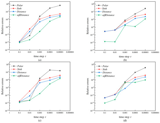
Figure 7. Relative errors for the domain integral using various methods at different time steps, with different point positions: (a) (1, 1), (b) (0.8, 0.8), (c) (0.5, 0), and (d) (0.5, 0.2).

As shown in Table 5 and Figure 7, the sinh transformation and the distance transformation, which are based on the (ρ, θ) coordinate system and the (α, β) coordinate system, respectively, significantly outperform the polar coordinate transformation in terms of accuracy. Moreover, the distance transformation yields superior results compared to the sinh transformation. As the source point approaches the vertex or edge of the quadrilateral element, progressively larger calculation errors are obtained. The issue arises from the formation of irregular sub-triangles during the subdivision of integration elements. Among all four methods, the (α, β) distance transformation exhibits optimal accuracy and stability.

4.5. Example 5

In this example, the calculation efficiency of different methods for computing the domain integral in (15) is considered. The integration element, source point positions, and other conditions are kept consistent with those in Example 4. The computation times for (15) using various methods running 10,000 times are exhibited in Table 6.

Table 6. The computation times for the domain integral in (15) using various methods running 10,000 times at different source point positions.

(1, 1)	τ = 0.1	τ = 0.01	τ = 0.001	τ = 0.0001	τ = 0.00001
Polar	3408 ms	3456 ms	3666 ms	3785 ms	3615 ms
Sinh	5365 ms	5423 ms	5650 ms	5629 ms	5574 ms
Distance	3939 ms	3920 ms	4067 ms	4105 ms	4122 ms
αβDistance	3324 ms	3337 ms	3488 ms	3622 ms	3532 ms
(0.8, 0.8)	τ = 0.1	τ = 0.01	τ = 0.001	τ = 0.0001	τ = 0.00001
Polar	6911 ms	6843 ms	6926 ms	7231 ms	7286 ms
Sinh	10,830 ms	10,729 ms	10,874 ms	11,150 ms	11,201 ms
Distance	8058 ms	10729 ms	8017 ms	8291 ms	8476 ms
αβDistance	9526 ms	6770 ms	6656 ms	6875 ms	7063 ms
(0.5, 0)	τ = 0.1	τ = 0.01	τ = 0.001	τ = 0.0001	τ = 0.00001
Polar	5269 ms	5246 ms	5663 ms	5380 ms	8236 ms
Sinh	8219 ms	8188 ms	8630 ms	8343 ms	8236 ms
Distance	6677 ms	5989 ms	6042 ms	6260 ms	5988 ms
αβDistance	5112 ms	5005 ms	5207 ms	7055 ms	5532 ms
(0.5, 0.2)	τ = 0.1	τ = 0.01	τ = 0.001	τ = 0.0001	τ = 0.00001
Polar	6808 ms	6863 ms	6937 ms	7204 ms	7117 ms
Sinh	10,666 ms	10,788 ms	10,953 ms	11,094 ms	11,090 ms
Distance	7738 ms	7745 ms	8115 ms	8096 ms	8133 ms
αβDistance	6649 ms	6597 ms	6853 ms	6830 ms	6926 ms

‘Polar’ denotes the polar coordinate transformation. ‘Sinh’ and ‘Distance’ refer to the sinh transformation and the new distance transformation, respectively. ‘αβDistance’ indicates the (α, β) distance method. The 20 × 20 Gaussian points are used in all methods. It is demonstrated in Table 6 that the computation efficiency of the (α, β) distance transformation is higher than that of the other three methods. Thus, higher computational accuracy is obtained by the proposed method with less calculation time.

4.6. Example 6

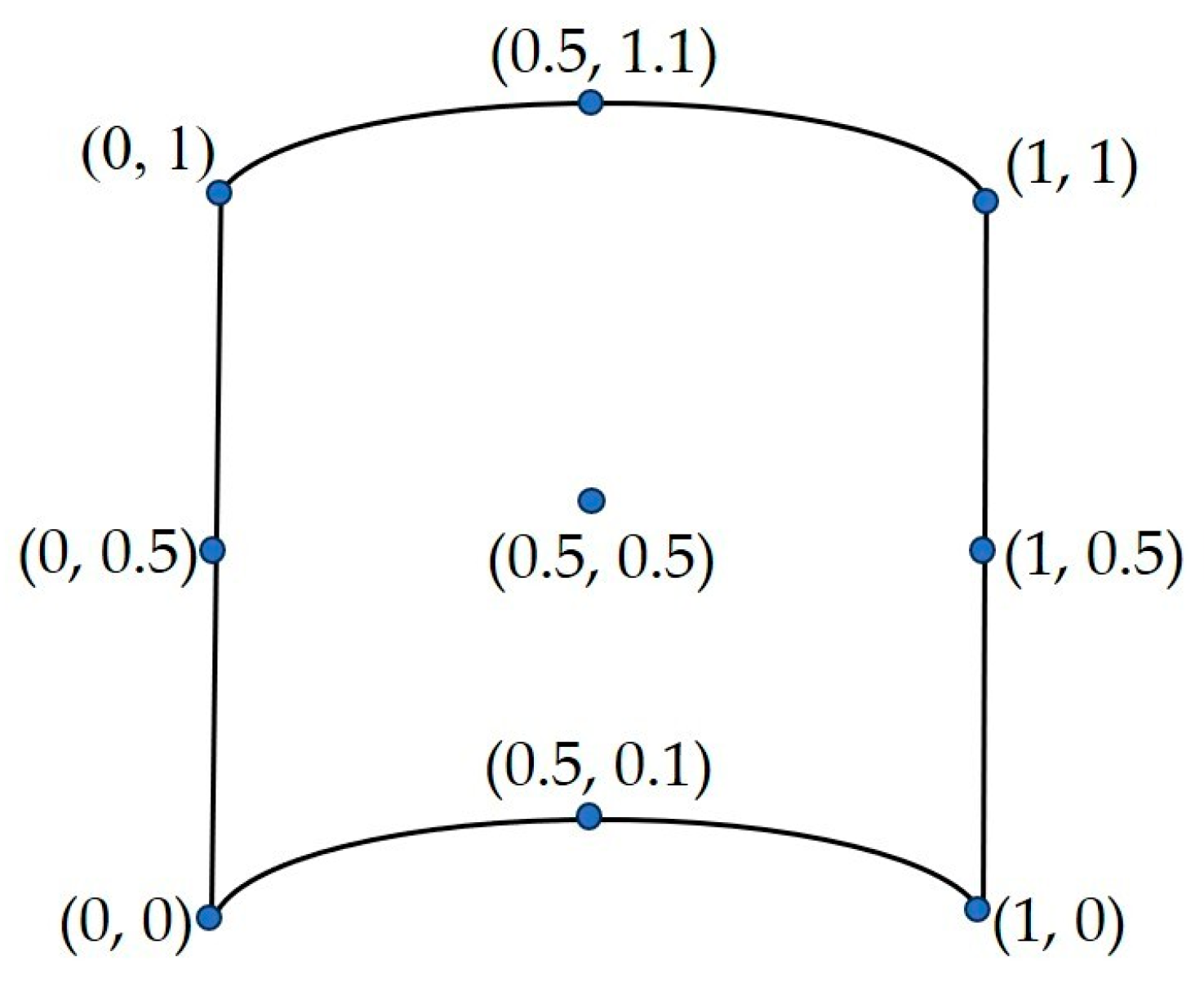
To further illustrate the advantages of the proposed method, a different quadrilateral integration element is employed. As shown in Figure 8, the curved quadrilateral element is characterized by nodal coordinates at (0, 0), (0, 1), (1, 1), (1, 0), (0, 0.5), (1, 0.5), (0.5, 0.1), (0.5, 1.1), and (0.5, 0.5) in this example. With the source point set at (0.5, 0.5) and various time step sizes, the results of the calculation are depicted in Table 7. ‘Direct’ indicates that Gaussian quadrature is applied directly. ‘Polar’ refers to the polar coordinate transformation. ‘Sinh’ and ‘Distance’ present the sinh transformation and the new distance transformation. ‘αβDistance’ denotes the (α, β) distance transformation. The 20 × 20 Gaussian points are used in all methods.

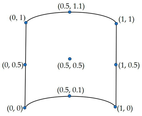
Figure 8. Coordinates for each node of the curved quadrilateral element.

Table 7. Relative errors for the integral in (15) on the curved element are obtained by various methods at different time steps, considering the source point positioned at (0.5, 0.5). Errors greater than 1 are indicated as E.

(0.5, 0.5)	τ = 0.1	τ = 0.01	τ = 0.001	τ = 0.0001	τ = 0.00001
Direct	3.100 × 10−15	2.126 × 10−14	5.385 × 10−3	E	E
Polar	2.067 × 10−16	1.814 × 10−14	3.769 × 10−9	2.283 × 10−4	1.078 × 10−1
Sinh	1.240 × 10−15	2.226 × 10−15	1.994 × 10−8	1.569 × 10−5	1.013 × 10−5
Distance	6.201 × 10−16	1.825 × 10−14	1.322 × 10−9	1.921 × 10−6	1.858 × 10−6
αβDistance	6.201 × 10−16	2.104 × 10−14	4.334 × 10−13	2.307 × 10−9	2.279 × 10−7

As revealed by the analysis in Table 7, significant calculation errors are produced by both the Gaussian quadrature method and the polar coordinate transformation when the value of τ is exceedingly small, making these methods unsuitable for such a condition. The analysis indicates that calculation accuracy is significantly improved by the sinh transformation and the new distance transformation. However, superior performance is demonstrated by the new distance transformation and the (α, β) distance transformation. Moreover, the proposed method achieves optimal results compared to all other methods.

4.7. Example 7

To underscore the broad applicability of the proposed method, the impact of interpolating the shape function on the results is evaluated in this example. The domain integral is considered as follows:

$$I_2={\displaystyle {\int }_{\Omega }\frac{N}{4\pi k\tau }\exp (-\frac{r^2}{4k\tau })}d\Omega$$

(17)

where N denotes the shape function of the curved quadrilateral element.

The integral is performed using the curved quadrilateral depicted in Figure 8, with the coordinate of the source point set at (0.5, 0.5). The relative errors of various methods at different time steps are compared in Table 8. ‘Direct’ indicates that Gaussian quadrature is applied directly. ‘Polar’ refers to the polar coordinate transformation. ‘Sinh’ and ‘Distance’ present the sinh transformation and the new distance transformation. ‘αβDistance’ denotes the (α, β) distance transformation. The 20 × 20 Gaussian points are used in all methods.

Table 8. Relative errors for the integral in (17) on the curved element are obtained using various methods at different time steps, with the source point located at (0.5, 0.5). Errors greater than 1 are indicated as E.

(0.5, 0.5)	τ = 0.1	τ = 0.01	τ = 0.001	τ = 0.0001	τ = 0.00001
Direct	4.383 × 10−15	4.699 × 10−14	5.954 × 10−3	E	E
Polar	2.789 × 10−15	2.238 × 10−15	5.021 × 10−9	2.253 × 10−4	1.079 × 10−1
Sinh	1.395 × 10−15	1.536 × 10−13	1.389 × 10−8	1.570 × 10−5	9.918 × 10−6
Distance	9.961 × 10−16	3.159 × 10−15	9.928 × 10−10	1.919 × 10−6	1.905 × 10−6
αβDistance	6.201 × 10−16	2.103 × 10−14	4.334 × 10−13	2.307 × 10−9	2.279 × 10−7

As can be observed from Table 8, the interpolation of the shape function into the domain integral slightly affects the calculation results. The calculation accuracy obtained using the proposed method is superior to that achieved with other methods. The results demonstrate that the (α, β) distance transformation achieves the highest level of accuracy, confirming its wide applicability.

5. Conclusions

An (α, β) distance transformation is proposed in this paper to compute 2D domain integrals that arise in the boundary element method for transient heat conduction problems. By employing the proposed method, the integrand is smoothed, and computational implementation is simplified. Furthermore, the singularity resulting from small time steps in the domain integral is effectively eliminated by the Jacobian of the (α, β) distance transformation. The numerical examples, which utilize different time step sizes, locations of source points, and element shapes, effectively validate the accuracy, stability, and broad applicability of the proposed method. The relative errors of the proposed method can be maintained at 10⁻⁵ until τ decreases to 10⁻⁵. Compared to the other four existing methods, the most accurate results are achieved by the new method, regardless of the time step size, the source point positions, and the shapes of the integration elements. Furthermore, the shortest calculation time for the domain integrals is required. Therefore, the (α, β) distance transformation can be efficiently applied to compute 2D domain integrals.

References

- Guo, Q.; Ye, P.X. Error analysis of moving least-squares method with non-identical sampling. Int. J. Comput. Math. 2019, 96, 767–781. [Google Scholar] [CrossRef]
- Gupta, A.; Sullivan, J.M., Jr.; Delgado, H.E. An efficient bem solution for three-dimensional transient heat conduction. Int. J. Numer. Methods Heat Fluid Flow 1995, 5, 327–340. [Google Scholar] [CrossRef]
- Goto, T.; Suzuki, M. A boundary integral equation method for nonlinear heat conduction problems with temperature-dependent material properties. Int. J. Heat Mass Transf. 1996, 39, 823–830. [Google Scholar] [CrossRef]
- Cui, X.Y.; Li, Z.C.; Feng, S.Z. Steady and transient heat transfer analysis using a stable node-based smoothed finite element method. Int. J. Therm. Sci. 2016, 110, 12–25. [Google Scholar] [CrossRef]
- AI-Khateeb, A. Efficient numerical solution for fuzzy time fractional convection diffusion equations using two explicit finite difference methods. Axioms 2024, 13, 221. [Google Scholar] [CrossRef]
- Ndou, N.; Dlamini, P.; Jacobs, B.A. Developing higher-order unconditionally positive finite difference methods for the advection diffusion reaction equations. Axioms 2024, 13, 247. [Google Scholar] [CrossRef]
- Gu, Y.; Hua, Q.S.; Zhang, C.Z. The generalized finite difference method for long-time transient heat conduction in 3D anisotropic composite materials. Appl. Math. Model. 2019, 71, 316–330. [Google Scholar] [CrossRef]
- Cheng, A.H.; Cheng, D.T. Heritage and early history of the boundary element method. Eng. Anal. Bound. Elem. 2005, 29, 268–302. [Google Scholar] [CrossRef]
- Liu, Y.J. Recent advances and emerging applications of the boundary element method. Appl. Mech. Rev. 2011, 64, 030802. [Google Scholar] [CrossRef]
- Yao, Z.H.; Wang, H.T. Large-scale thermal analysis of fiber composites using a line-inclusion model by the fast boundary element method. Eng. Anal. Bound. Elem. 2013, 37, 319–326. [Google Scholar]
- Yu, B.; Cao, G.Y.; Gong, Y.P.; Ren, S.H.; Dong, C.Y. IG-DRBEM of three-dimensional transient heat conduction problems. Eng. Anal. Bound. Elem. 2021, 128, 298–309. [Google Scholar] [CrossRef]
- Yu, B.; Cao, G.Y.; Huo, W.D.; Zhou, H.L.; Atroshchenko, E. Isogeometric dual reciprocity boundary element method for solving transient heat conduction problems with heat sources. J. Comput. Appl. Math. 2021, 385, 113197. [Google Scholar] [CrossRef]
- Yu, B.; Cao, G.Y.; Meng, Z.; Gong, Y.P.; Dong, C.Y. Three-dimensional transient heat conduction problems in FGMs via IG-DRBEM. Comput. Methods Appl. Mech. Eng. 2021, 384, 113958. [Google Scholar] [CrossRef]
- Erhart, K.; Divo, E.; Kassab, A.J. A parallel domain decomposition boundary element method approach for the solution of large-scale transient heat conduction problems. Eng. Anal. Bound. Elem. 2006, 30, 553–563. [Google Scholar] [CrossRef]
- Feng, W.Z.; Yang, K.; Cui, M.; Gao, X.W. Analytically-integrated radial integration BEM for solving transient heat conduction problems. Int. Commun. Heat Mass Transf. 2016, 79, 21–30. [Google Scholar] [CrossRef]
- Feng, W.Z.; Gao, L.F.; Du, J.M.; Qian, W.; Gao, X.W. A meshless interface integral BEM for solving heat conduction in multi-non-homogeneous media with multiple heat sources. Int. Commun. Heat Mass Transf. 2019, 104, 70–82. [Google Scholar] [CrossRef]
- Zhou, F.L.; Xie, G.Z.; Zhang, J.M.; Zheng, X.S. Transient heat conduction analysis of solids with small open-ended tubular cavities by boundary face method. Eng. Anal. Bound. Elem. 2013, 37, 542–550. [Google Scholar] [CrossRef]
- Li, G.Y.; Guo, S.P.; Zhang, J.M.; Li, Y.; Han, L. Transient heat conduction analysis of functionally graded materials by a multiple reciprocity boundary face method. Eng. Anal. Bound. Elem. 2015, 60, 81–88. [Google Scholar] [CrossRef]
- Sharp, S. Stability analysis for boundary element methods for the diffusion equation. Appl. Math. Model. 1986, 10, 41–48. [Google Scholar] [CrossRef]
- Piece, A.P.; Askar, A.; Rabitz, H. Convergence properties of a class of boundary element approximations to linear diffusion problems with localized nonlinear reactions. Numer. Methods Partial. Differ. Equ. 1990, 6, 75–108. [Google Scholar]
- Dargush, G.F.; Grigoriev, M.M. Higher-order boundary element methods for transient diffusion problems. Part II: Singular flux formulation. Int. J. Numer. Methods. Eng. 2002, 55, 41–54. [Google Scholar] [CrossRef]
- Dong, Y.Q.; Zhang, J.M.; Xie, G.Z.; Chen, C.J.; Li, Y.; Hu, X.; Li, G.Y. A general algorithm for evaluating domain integrals in 2D boundary element method for transient heat conduction. Int. J. Comput. Methods 2015, 12, 1550010. [Google Scholar] [CrossRef]
- Dong, Y.Q.; Zhang, J.M.; Xie, G.Z.; Lu, C.J.; Han, L.; Wang, P. A general algorithm for the numerical evaluation of domain integrals in 3D boundary element method for transient heat conduction. Eng. Anal. Bound. Elem. 2015, 51, 30–36. [Google Scholar] [CrossRef]
- Gao, X.W. The radial integration method for evaluation of domain integrals with boundary-only discretization. Eng. Anal. Bound. Elem. 2002, 26, 905–916. [Google Scholar] [CrossRef]
- Yang, K.; Gao, X.W. Radial integration BEM for transient heat conduction problems. Eng. Anal. Bound. Elem. 2010, 34, 557–563. [Google Scholar] [CrossRef]
- Yang, K.; Peng, H.F.; Wang, J.; Xing, C.H.; Gao, X.W. Radial integration BEM for solving transient nonlinear heat conduction with temperature-dependent conductivity. Int. J. Heat Mass Transf. 2017, 108, 1551–1559. [Google Scholar] [CrossRef]
- Dong, Y.Q. Evaluating 2D domain integrals by sinh transformation for transient heat conduction problem. J. Phys. Conf. Ser. 2019, 1300, 012095. [Google Scholar] [CrossRef]
- Dong, Y.Q.; Sun, H.B.; Tan, Z.X. A new distance transformation method of estimating domain integrals directly in boundary integral equation for transient heat conduction problems. Eng. Anal. Bound. Elem. 2024, 160, 45–51. [Google Scholar] [CrossRef]
- Johnston, P.R.; Elliott, D. A sinh transformation for evaluating nearly singular boundary element integrals. Int. Numer. Meth. Eng. 2005, 62, 564–578. [Google Scholar] [CrossRef]
- Gu, Y.; Chen, W.; Zhang, C.Z. The sinh transformation for evaluating nearly singular boundary element integrals over high-order geometry elements. Eng. Anal. Bound. Elem. 2013, 37, 301–308. [Google Scholar] [CrossRef]
- Zhang, Y.M.; Gong, Y.P.; Gao, X.W. Calculation of 2D nearly singular integrals over high-order geometry elements using the sinh transformation. Eng. Anal. Bound. Elem. 2015, 60, 144–153. [Google Scholar] [CrossRef]
- Ma, H.; Kamiya, N. Distance transformation for the numerical evaluation of near singular boundary integrals with various kernels in boundary element method. Eng. Anal. Bound. Elem. 2002, 26, 329–339. [Google Scholar] [CrossRef]
- Ma, H.; Kamiya, N. A general algorithm for the numerical evaluation of nearly singular boundary integrals of various orders for two- and three- dimensional elasticity. Comput. Mech. 2002, 29, 277–288. [Google Scholar] [CrossRef]
- Qin, X.Y.; Zhang, J.M.; Xie, G.Z.; Zhou, F.L.; Li, G.Y. A general algorithm for the numerical evaluation of nearly singular integrals on 3D boundary element. J. Comput. Appl. Math. 2011, 235, 4174–4186. [Google Scholar] [CrossRef]
- Zhang, J.M.; Qin, X.Y.; Han, X.; Li, G.Y. A boundary face method for potential problems in three dimensions. Int. J. Numer. Meth. Eng. 2009, 80, 320–337. [Google Scholar] [CrossRef]
- Gao, X.W.; Yang, K.; Wang, J. An adaptive element subdivision technique for evaluation of various 2D singular boundary integrals. Eng. Anal. Bound. Elem. 2008, 32, 692–696. [Google Scholar] [CrossRef]
Disclaimer/Publisher’s Note: The statements, opinions and data contained in all publications are solely those of the individual author(s) and contributor(s) and not of MDPI and/or the editor(s). MDPI and/or the editor(s) disclaim responsibility for any injury to people or property resulting from any ideas, methods, instructions or products referred to in the content. |
© 2024 by the authors. Licensee MDPI, Basel, Switzerland. This article is an open access article distributed under the terms and conditions of the Creative Commons Attribution (CC BY) license (https://creativecommons.org/licenses/by/4.0/).