Adding a Degree of Certainty to Deductions in a Fuzzy Temporal Constraint Prolog: FTCProlog

Abstract

The management of time is essential in most AI-related applications. In addition, we know that temporal information is often not precise. In fact, in most cases, it is necessary to deal with imprecision and/or uncertainty. On the other hand, there is the need to handle the implicit common-sense information present in many temporal statements. In this paper, we present FTCProlog, a logic programming language capable of handling fuzzy temporal constraints soundly and efficiently. The main difference of FTCProlog with respect to its predecessor, PROLogic, is its ability to associate a certainty index with deductions obtained through SLD-resolution. This resolution is based on a proposal within the theoretical logical framework FTCLogic. This model integrates a first-order logic based on possibilistic logic with the Fuzzy Temporal Constraint Networks (FTCNs) that allow efficient time management. The calculation of the certainty index can be useful in applications where one wants to verify the extent to which the times elapsed between certain events follow a given temporal pattern. In this paper, we demonstrate that the calculation of this index respects the properties of the theoretical model regarding its semantics. FTCProlog is implemented in Haskell.

1. Introduction

In the field of artificial intelligence and expert systems, there are multiple models for reasoning about the time of occurrence of events or the temporal constraints between them. Many proposals include the ability to handle uncertainty and/or imprecision in time-related facts. For example, Allen’s temporal relations [1] are extended in the temporal reasoning intelligent system Fuzz-time [2] to allow fuzzy time intervals to be compared. Furthermore, this system allows this type of reasoning to be incorporated in a database. The Possibility Theory [3] has also been applied in temporal reasoning in logical models such as Timed Possibilistic Logic [4] or algebraic models such as Fuzzy Temporal Constraint Networks or FTCNs [5,6,7], where possibility theory is used as a formalism to represent imprecision in metric constraints between temporal instants. The temporal reasoner Fuzzy Temporal Information Management Engine or FuzzyTIME [8] uses the FTCN model but adds a module that allows for the representation of points and intervals, quantitative and qualitative relations, and imprecision and uncertainty. FuzzyTIME is capable of determining temporal consistency, searching for solutions and resolving queries.

The FTCN model allows for very efficient management of fuzzy temporal reasoning. However, when the goal is to provide a framework that ensures soundness and completeness in reasoning, the use of formal logic and automated reasoning becomes of great interest. Numerous works can be found that provide variations of logical deduction with the ability to manipulate time [9], such as the temporal propositional logic included in the MTPL system [10], or the modal temporal logics PNL [11] or GTL [12]. On the other hand, in [13], a propositional temporal language based on fuzzy temporal constraints with consistent inference rules is proposed, while in [14], a first-order programming language based on possibilistic logic is proposed for reasoning in environments with uncertainty and lack of information, using a modus ponens-type rule. Another first-order language based on LTL [15] is also proposed, which improves the treatment of variables in temporal logic programming of the STeLP tool [16].

From our point of view, the combination of expressiveness and guarantees provided by a logical model, along with the efficiency in handling time that can be achieved with an algebraic model such as an FTCN, provides the most suitable framework for reasoning in contexts where knowledge of the domain is as important as the temporal constraints (often fuzzy or uncertain) between data or events associated with that domain.

The only model we know of that provides a reasoning mechanism (temporal resolution) that efficiently processes temporal constraints while making deductions associated with domain data is the first-order fuzzy temporal logic model FTCLogic [17]. FTCLogic is based on the FTCN model and possibilistic logic [18,19]. It has high expressiveness, is sufficiently general in the sense that it is adaptable to any application area, has an efficient inference rule (by combining the resolution principle with the minimization of FTCN networks), and is sound and complete, which guarantees correctness in deductions. These characteristics led to the implementation of the PROLogic language [20], which is an implementation of FTCLogic that looks like Prolog. Although there are other proposals for implementing a Temporal Prolog, such as [21,22,23,24], they do not include efficient, consistent, and homogeneous handling of temporal and non-temporal information, as proposed in PROLogic.

The resurgence of artificial intelligence has opened up new areas of significant interest, such as Machine Learning or Explainable Artificial Intelligence (XAI) [25], emphasizing the necessity of integrating models capable of effectively managing uncertainty [26] and temporal information. For instance, in [27], the researchers investigated a safe learning problem that satisfied linear temporal logic (LTL) constraints. On the other hand, in [28], the FTCN model was employed to detect inconsistencies within pre-trained language models in a specific application domain of a conversational agent. This agent is designed to provide users with natural and accurate explanations. In [29], a time-dependent explainable artificial intelligent system is introduced. It is based on novel temporal type-2 fuzzy sets to analyze real-life processes accounting for their time dependencies. On the other hand, in [30], the authors propose enhancing language models with temporal logical induction capability using a method they call LECTER, or Logic Induction Enhanced Contextualized Temporal Reasoning. Techniques from Inductive Logic Programming (ILP) are applied to learn logic rules by generalizing from both temporal and relational data in [31], where the authors propose what they term Temporal Inductive Logic Reasoning (TILR). Finally, in [32], we can find a comprehensive survey of research on temporal reasoning for automatic temporal information extraction from text.

In Figure 1, we present a PRISMA flow chart [33,34] to illustrate the process we have followed for selecting and evaluating studies on Fuzzy Logic applied to Temporal Reasoning, focusing on models capable of dealing with temporal constraints. As can be seen, we have been particularly interested in the use of these models in the context of new AI applications.

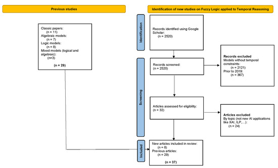
Figure 1. PRISMA flow diagram for literature search on fuzzy constraint logic applied to temporal reasoning for new applications in AI. Search conducted on Google Scholar.

In this work, we present the tool FTCProlog. The methodology followed for its implementation begins with the theoretical definition of the temporal reasoning model FTCLogic. This theoretical model makes deductions with clauses, each of which is associated with an FTCN. At each step of the refutation process, the fuzzy constraints of these networks intersect with each other, so that the information about the time elapsed between two events becomes increasingly precise. If an inconsistent network is obtained, the process stops, and no deduction is made. The PROLogic tool implements this process, as we mentioned earlier. It is a logic programming language based on FTCLogic and implemented in Haskell. However, in certain applications, it may be of interest to know to what extent the temporal constraints in a given temporal pattern resemble those that relate to the occurrence of specific events. In this context, we introduce a modified version of PROLogic, which we named FTCProlog, that allows a certainty index to be associated with each SLD-refutation. This measure is obtained by calculating the compatibility of the fuzzy constraints involved in the resolution process. We will demonstrate that this measure respects the soundness and completeness properties proven for FTCLogic. Additionally, we study the behavior of this index by introducing a simple example in FTCProlog.

This paper has been organized as follows. In Section 2, we explain, through the use of simple examples, the theoretical foundations of the tool we propose: FTCLogic. We will begin by presenting the main concepts of FTCN and summarizing the syntax and semantics of FTCLogic. A complete definition of FTCLogic can be found in [17]. The PROLogic language is the implementation of the resolution principle of this logic in Haskell. In Section 3, we will use some examples to address the main issues associated with the use of PROLogic programs. The complete description of the tool can be found in [20]. In Section 4, we will present the main features of FTCProlog, paying special attention to what sets this application apart from its predecessor PROLogic. In Section 4.1, we define a certainty measure associated with each deduction. In Section 4.2, we demonstrate the consistency of this measure and we outline how its calculation has been implemented, while in Section 4.3, we study the values obtained for different instances of an example in the context of marketing on an online sales page. Finally, Section 5 offers the main conclusions.

2. FTCLogic

We begin by summarizing some basic FTCLogic issues through a simple example. The full definitions of the syntax, semantics, and resolution principle of FTCLogic can be found in [17].

2.1. Basic Notions of FTCN

Since FTCNs are an essential part of FTCLogic clauses, we start by exposing the most basic concepts about them. A complete explanation can be found in [5,6,7].

Definition 1. 

A Fuzzy Temporal Constraint Network (FTCN) $\mathcal{N}=<X,L>$ is a pair made up of a finite set of $n+1$ temporal variables $X=\{X_0,X_1\dots X_n\}$ and a finite set of fuzzy temporal binary constraints among them $L=\left\{L_{ij}\right|i,j\le n\}$

The possible values of the difference between the variables $X_j$ and $X_i$ can be described by a binary constraint $L_{ij}$, defined by a possibility distribution ${\pi }_{ij}$ over the set of real values $\mathbb{R}$. In case the temporal constraint between the two variables $X_i$ and $X_j$ is not known, we assume that there exists a universal constraint given by ${\pi }_U\left(x\right)=1$, $\forall x$∈$\mathbb{R}$. To represent an FTCN, a directed graph is generally used. In this graph, each node corresponds to a variable while the arcs represent a binary constraint between two variables.

Definition 2. 

A $\sigma$-possible solution of FTCN $\mathcal{N}$ is defined as an n-tuple $s=(x_1,\dots x_n)\in {\mathbb{R}}^n$ which verifies ${\pi }_S\left(s\right)=\sigma$, where ${\pi }_S$ is:

$${\pi }_S\left(s\right)=\underset{i,j\le n}{min}{\pi }_{ij}(x_j-x_i).$$

If there is at least one absolutely possible solution, the FTCN is said to be consistent . This case occurs when the possibility distribution ${\pi }_S$ is normalized.

We say that two FTCNs are equivalent if they define the same n-ary fuzzy relation. Two equivalent networks can differ in some constraints $L_{ij}$. This is because there may be other constraints that act on the variables $X_i$ and $X_j$. That is, a more precise implicit constraint between these variables can be induced by the rest of the constraints. If, to obtain an induced constraint $M_{ij}$ between the variables $X_i$ and $X_j$, all the other constraints of FTCN have been used, this constraint is minimal with respect to inclusion. $M_{ij}$ contains all the information available on the network. Given an FTCN $\mathcal{N}$, we are interested in an equivalent FTCN $\mathcal{M}$, in which the minimal constraints are shown explicitly. This network is called the minimal network and its constraints $M_{ij}$ are obtained by exhaustive constraint propagation. The process of obtaining the minimal network can be implemented using a fuzzy version of the path-consistency algorithm [35]. This algorithm will also serve to detect temporal inconsistencies in the network.

We assume convex and normalized possibility distributions. This allows us to consider constraints as fuzzy numbers representable by means of trapezoidal distribution [36]. These can be defined by four parameters $(\alpha ,\beta ,\gamma ,\delta )$. In this way, arithmetic operations can be performed efficiently.

The following definitions are important for the definition of FTCLogic:

Definition 3. 

Given two FTCN networks ρ and ${\rho }^{\prime }$ defined on the same set of nodes, we can say that$\rho$ is included in ${\rho }^{\prime }$ , and we denote it as $\rho ◃{\rho }^{\prime }$ if, for each pair of nodes $n_i$ and $n_j$ belonging to both networks, it is fulfilled that ${\pi }_{ij}\subset {\pi }_{ij}^{\prime }$, where ${\pi }_{ij}$ is the possibility distribution between $n_i$ and $n_j$ in the network ρ and ${\pi }_{ij}^{\prime }$ is that corresponding to ${\rho }^{\prime }$ for the same nodes. This means that ${\pi }_{ij}\left(x\right)\le {\pi }_{ij}^{\prime }\left(x\right),\forall x\in \mathbb{R}$.

Definition 4. 

Given two FTCN networks ρ and ${\rho }^{\prime }$ defined on the same set of nodes, we use $\rho \cap {\rho }^{\prime }$ to denote a new network obtained by making the fuzzy intersection between ${\pi }_{ij}$ and ${\pi }_{ij}^{\prime }$ for each pair of nodes $n_i$ and $n_j$ belonging to both networks, with ${\pi }_{ij}$ being the possibility distribution between $n_i$ and $n_j$ in the network ρ and ${\pi }_{ij}^{\prime }$ is that corresponding to ${\rho }^{\prime }$ for the same nodes.

Definition 5. 

Given several networks ${\rho }_1$, …, ${\rho }_n$, defined on the same set of nodes, we give the name maximal network to a new network that obtains the ${\pi }_{ij}$ possibility distributions associated with each pair of nodes $n_i$ and $n_j$ as the fuzzy union of ${\pi }_{ij}^1$, ${\pi }_{ij}^2$, …and ${\pi }_{ij}^n$, where ${\pi }_{ij}^1$, ${\pi }_{ij}^2$, …and ${\pi }_{ij}^n$ are the possibility distributions between $n_i$ and $n_j$ in the ${\rho }_1$, …and ${\rho }_n$ networks, respectively.

The fuzzy union can be defined as follows:

$({\alpha }_1,{\beta }_1,{\gamma }_1,{\delta }_1)\bigcup ({\alpha }_2,{\beta }_2,{\gamma }_2,{\delta }_2)=(min\{{\alpha }_1,{\alpha }_2\},min\{{\beta }_1,{\beta }_2\},max\{{\gamma }_1,{\gamma }_2\},max\{{\delta }_1,{\delta }_2\}).$

In the following example, we can see how an FTCN is used to express the temporal relationship between three events related to the occurrence of close contact in a case of COVID-19 transmission.

Example 1. 

Let us suppose we want to use an FTCN to establish the temporal relationship between the occurrence of three events: the establishment of contact between two people (which occurred at a time we call @T_CONT), the onset of symptoms of COVID-19 infection in one of these two people (which occurred at time @T_SS), and the moment this person was considered a confirmed case of the disease (corresponding to time @T_CC).

To consider the contact between these two people as a close contact, based on [37], we could establish that the contact should occur between approximately 3 days before and approximately 7 days after the onset of symptoms for contagion to exist. On the other hand, this contact can occur before, at the same time as, or after one of them is considered a confirmed case of the disease.

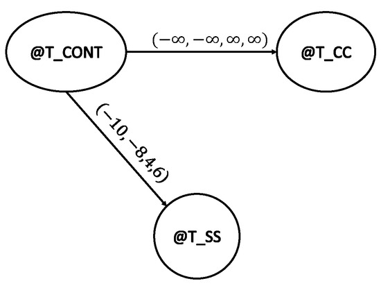
The network in Figure 2 establishes these temporal constraints, which could be considered as a kind of temporal pattern associated with the concept of close contact. If we consider the fuzzy number (−10, −8, 4, 6) as a possible translation of the quantity indicated by the expression “between approximately 3 days before and approximately 7 days after”, the constraint between @T_CONT and @T_SS establishes this amount of time as the approximate temporal distance between the occurrence of contact and the onset of symptoms. On the other hand, since the contact (@T_CONT) could occur before, at the same time as, or after the determination of a confirmed case (@T_CC), any amount of time between @T_CONT and @T_CC would be consistent. This corresponds to the constraint $(-\infty ,-\infty ,\infty ,\infty )$ that could be labeled with the expression “before or at the same time or after”.

Figure 2. Temporal constraints between temporal variables @T_CONT, @T_CC, and @T_SS.

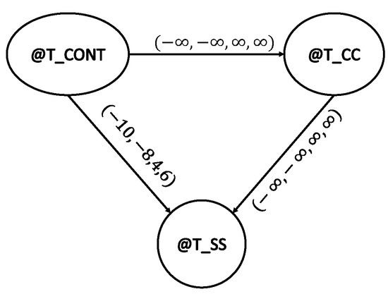
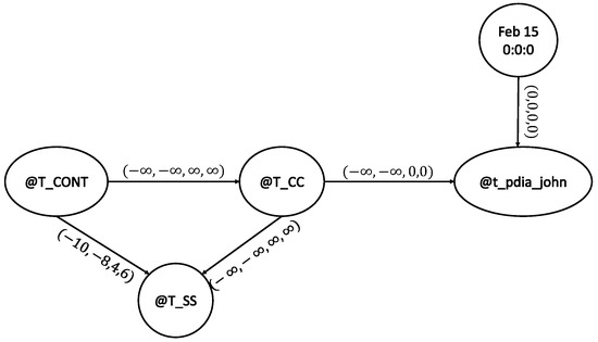
The FTCN in Figure 3 corresponds to the minimization of the FTCN in Figure 2.

Figure 3. ${\rho }_2$: Minimal FTCN equivalent to the network in Figure 2.

2.2. Syntax of FTCLogic

Let $\mathcal{L}$ represent a classic first-order language.

Definition 6. 

The set $\mathcal{C}$ of FTCClauses is as a set of tuples $(\varsigma ,\rho )$, where ς is a Horn clause of $\mathcal{L}$, in which k temporal variables appear, and ρ is the FTCN that relates them.

Each FTCClause has an associated Fuzzy Temporal Constraint Network or FTCN as a second component. We can write an FTCClause without non-temporal information as $(Time,\rho )$, where $Time$ is a special predicate. Furthermore, we can write a FTCClause without temporal information as $(\varsigma ,{\rho }_U)$, where ${\rho }_U$ corresponds to a network in which all constraints are ${\pi }_U$, that is, a network without significant temporal information (see Section 2.1).

We use the FTCLogic syntax in the following example.

Example 2. 

Let us suppose that on 15 November 2022, John tested positive for COVID-19 in an active infection diagnostic test (PDIA). John stated that he started experiencing symptoms compatible with the disease approximately 4 days prior to the positive test. The day before the onset of symptoms, John met with his friend Louis and they went out for dinner. Additionally, on 5 November, John went to the movies with Peter.

The syntax of FTCLogic allows us to express these events with the following fact clauses:

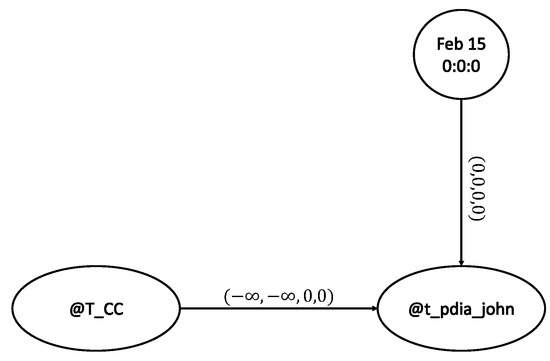
• A predicate indicating that John tested positive in an active infection diagnostic test (PDIA) for COVID-19 at the instant $@t\_pdia\_john$, associated with the network ${\rho }_1$ in Figure 4. This network specifies that the test was carried out on 15 November at 0:00 h. This is determined by the restriction labeled with the fuzzy number $(0,0,0,0)$ between the indicated date and the instant $@t\_pdia\_john$:
  

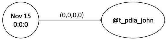  Figure 4. ${\rho }_1$.
  $(pdia(john,covid,positive,@t\_pdia\_john),{\rho }_1)$
• A predicate indicating that John started experiencing COVID-19 symptoms at the time $@t\_sym\_john$. The network ${\rho }_U$, associated with this fact, corresponds to the network in which all the constraints are ${\pi }_U$, that is, it is a network without information:
  $(start\_sym(john,covid,@t\_sym\_john),{\rho }_U)$
• A predicate indicating that Louis had a contact with John at the time $@t\_cont\_jl$. The associated network is ${\rho }_U$, as before:
  $(contact(john,louis,@t\_cont\_jl),{\rho }_U)$
• A predicate indicating that Peter had contact with John at the time $@t\_cont\_jp$:
  $(contact(john,peter,@t\_cont\_jp),{\rho }_U)$

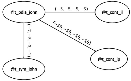
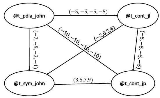
In FTCLogic, the temporal information contained in the example can be expressed with a clause whose non-temporal component consists simply of the $Time$ predicate, while the temporal part is a network, the network ${\rho }_{T1}$, which includes all the temporal constraints between the previous facts:

$(Time,{\rho }_{T1})$

We can see the network ${\rho }_{T1}$ in Figure 5 before minimization and in Figure 6 after minimization.

Figure 5. ${\rho }_{T1}$ not minimized.

Figure 6. ${\rho }_{T1}$ minimized.

Suppose the fuzzy number (−7, −5, −3, −1) corresponds to the fuzzy temporal constraint “approximately 4 days after”. (−5,−5,−5,−5) and (−10,−10,−10,−10) correspond to the precise constraints “5 days after” and “10 days after”, respectively.

On the other hand, a possible pattern to confirm the existence of close contact of a person P2 with a confirmed case P1 of COVID-19 infection at the time $@T\_CC$ could be expressed with the following rule clause:

$(close\_contact(P1,P2,covid,@T\_CONT)\vee$

$\neg confirmed\_case(P1,covid,@T\_CC)\vee$

$\neg start\_sym(P1,covid,@T\_SS)\vee$

$\neg contact(P1,P2,@T\_CONT),{\rho }_2)$

where ${\rho }_2$ corresponds to the FTCN in Figure 3.

As we indicated in Example 1, we understand that a COVID-19 patient can transmit the disease between approximately 3 days before the onset of symptoms and approximately 7 days after this fact [37].

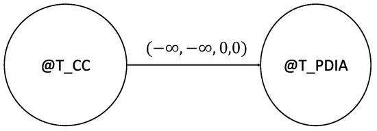
The start_sym and contact predicates correspond to basic facts. However, the predicate confirmed_case associated with a patient P depends on the existence of a positive pdia . This is expressed through the following clause:

$(confirmed\_case(P,covid,@T\_CC)\vee$

$\neg pdia(P,covid,positive,@T\_PDIA),{\rho }_3)$

where ${\rho }_3$ corresponds to the FTCN in Figure 7.

Figure 7. ${\rho }_3$.

The constraint in this network indicates that a disease case becomes a confirmed case upon obtaining a positive pdia , that is, the constraint between a confirmed case and pdia is simultaneous or subsequent.

2.3. Semantics of FTCLogic

As we know, in an FTCLogic-clause, $(\varsigma ,\rho )$, the component $\rho$ is an FTCN. Therefore, as we saw in Section 2.1, we can use the constraints of $\rho$ to obtain the possibility distribution ${\pi }_S$, which assigns a degree of possibility to each resolved tuple $s=(x_1,\dots ,x_n)$. On the other hand, each of the $x_i$ could also represent the value of a term in one of the predicates of $\varsigma$. Hence, it is reasonable to inquire to what extent the temporal knowledge contained in $\rho$ implies the certainty of the clause $\varsigma$.

In [17], we can find a detailed exposition of the semantics of FTCLogic. Here, we retrieve some definitions that we will need later:

Definition 7. 

Let Ω be the set of possible interpretations for the language $\mathcal{L}$. We define an interpretation for a FTCClause $(\varsigma ,\rho )$ as a pair $\tau =(\omega ,s)$, where $\omega \in \mathrm{\Omega }$, and $s=(x_1,\dots ,x_n)$ is a possible tuple solution of ρ.

Definition 8. 

An interpretation for a FTCClause $(\varsigma ,\rho )$, $\tau =(\omega ,s)$, where $\omega \in \mathrm{\Omega }$, and $s=(x_1,\dots ,x_n)$ is a possible tuple solution of ρ, is a model of $C=(\varsigma ,\rho )$ and is denoted with $\tau \vDash C$, if $\omega \vDash \varsigma$ (in the classic sense), and the values for each $x_i$ are compatible with ω.

By compatible, we understand that those values correspond to a node that appears in a predicate of ς which is certain under ω, or those values that correspond to a node that do not appear in any predicate of t ς.

Definition 9. 

We define the network possibility measure ${\mathrm{\Pi }}_{\mathcal{N}}$, induced by ${\pi }_S$, as a function from $\mathcal{C}$ to $[0,1]$, defined by

${\mathrm{\Pi }}_{\mathcal{N}}\left((\varsigma ,\rho )\right)=sup\{{\pi }_S\left(s\right),\tau =(\omega ,s),\tau \vDash (\varsigma ,\rho )\}$

${\pi }_S$ defines the fuzzy set S of possible solutions of ρ and $\omega \in \mathrm{\Omega }$.

${\mathrm{\Pi }}_{\mathcal{N}}$ indicates the degree to which the knowledge of the fuzzy temporal constraints among the temporal variables of $\rho$ is compatible with $\varsigma$.

Definition 10. 

We define the network necessity measure $N_{\mathcal{N}}$, induced by ${\pi }_S$, as a function from $\mathcal{C}$ to $[0,1]$, defined by

$N_{\mathcal{N}}\left((\varsigma ,\rho )\right)=inf\{1-{\pi }_S\left(s\right),\tau =(\omega ,s),\tau \vDash (\neg \varsigma ,\rho )\}$

${\pi }_S$ defines the fuzzy set S of possible solutions of ρ and $\omega \in \mathrm{\Omega }$.

$N_{\mathcal{N}}$ indicates the degree to which the knowledge of the fuzzy temporal constraints among the temporal variables of $\rho$ implies that $\varsigma$ is certain.

We will base the definition of the semantics on this last measure:

Definition 11. 

A clause $C=(\varsigma ,\rho )$ is γ- certain if ς is certain in the classic sense and $N_{\mathcal{N}}\left(C\right)=\gamma$.

Definition 12. 

Given a set of FTCClauses $\mathcal{C}=\{C_1,C_2,...,C_n\}$, and an FTCClause C, we will say that C is a logical consequence of $\mathcal{C}$, and it is denoted as $\mathcal{C}\vDash C$ if, for each interpretation τ that makes ${\gamma }_i$-certain to every $C_i$ and γ-certain to C, it is fulfilled that $\gamma \ge max\{{\gamma }_1,...,{\gamma }_n\}$.

The deduction problem consists in finding, given a set of classic clauses ${\mathcal{C}}^{*}$ and the clause $\varsigma$, the maximal FTCN network (see Definition 5) associated with $\varsigma$. We therefore define $Val(\varsigma ,\mathcal{C})$ as follows:

Definition 13. 

$Val\left((\varsigma ,\mathcal{C})\right)=N_{\mathcal{N}}(\varsigma ,{\rho }_{max})$, such that ${\rho }_{max}$ is the maximal network obtained from all the ${\rho }_i$ such that $\mathcal{C}\vDash (\varsigma ,{\rho }_i)$.

Finally, when a set of $FTCClauses$ is partially inconsistent (i.e., not in the classic sense), it is in our interest to define the degree of inconsistency $Incons\left(\mathcal{C}\right)$, which we can achieve as follows:

Definition 14. 

$Incons\left(\mathcal{C}\right)=N_{\mathcal{N}}\left((\perp ,{\rho }_{max})\right)$.

2.4. Resolution Principle in FTCLogic

To apply the FTCLogic resolution principle, based on that of [38], we consider the $\mathcal{L}$ clauses as Horn clauses. That is, they correspond to one of the following types:

• Fact clauses : $(p(...),{\rho }_i)$;
• Rules clauses : $(p_1(...)\vee \neg p_2(...)\vee ...\vee \neg p_n,{\rho }_i)$;
• Goal clauses : $(\neg p_1(...)\vee \neg p_2(...)\vee ...\vee \neg p_n,{\rho }_i)$.

where ${\rho }_i$ is the FTCN associated with each $\mathcal{L}$-clause.

In the unification process, the following formula is applied:

$((p_1(...)\vee \neg p_2(...)\vee ...\vee \neg p_n(...))$, $\rho )$

$((\neg p_1(...)\vee \neg p_{n+1}(...)\vee ...\vee \neg p_m(...))$, ${\rho }^{\prime })$

$\overline{((\neg p_2(...)\vee ...\vee \neg p_n(...)\vee \neg p_{n+1}(...)\vee ...\vee \neg p_m(...))\sigma ,{\rho }^{″})}$

where $\sigma$ is the MGU (Most General Unifier) and ${\rho }^{″}$ is the FTCN network associated with the resolvent clause.

${\rho }^{″}$ is calculated as follows: we call ${\pi }_{ij}$ the possibility distribution between $n_i$ and $n_j$ in $\rho$, and ${\pi }_{ij}^{\prime }$ the possibility distribution in ${\rho }^{\prime }$ for the same nodes. So, ${\rho }^{″}$ will be a new network obtained by performing the fuzzy intersection between ${\pi }_{ij}$ and ${\pi }_{ij}^{\prime }$ for each pair of nodes $n_i$ and $n_j$ belonging to networks $\rho$ and ${\rho }^{\prime }$.

The resolution process will consist of seeking a refutation by applying the resolution rule repeatedly.

We use the special clause $(Time,{\rho }_T)$ to be able to handle temporal information without explicitly associating it with non-temporal information. For this clause to be taken into account in the refutation by the resolution process, it is necessary to add the literal $\neg Time$ to the goal clause.

We will also see this in the example below.

Example 3. 

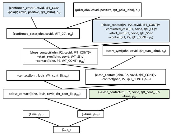
Continuing Example 2, we can deduce that Louis is John’s close contact using the resolution process we summarized in Figure 8.

Figure 8. Refutation by resolution to verify that Louis is John’s close contact.

We have colored the rules clauses in blue. On the other hand, we indicate the goal clause in green. The rest (blank) are fact clauses or resolvent clauses.

The ${\rho }_1$, ${\rho }_2$, ${\rho }_3$, and ${\rho }_{T1}$ networks are those of Figure 3, Figure 4, Figure 6, and Figure 7. We present the obtained networks ${\rho }_{31}$, ${\rho }_{312}$, and ${\rho }_{\lambda }$ in Figure 9, Figure 10 and Figure 11.

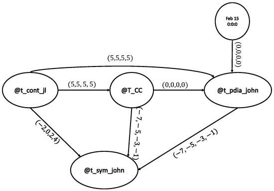
Figure 9. ${\rho }_{31}$.

Figure 10. ${\rho }_{312}$.

Figure 11. ${\rho }_{\lambda }$.

If we proceed in the same way with Peter, the resolution does not reach refutation. An inconsistency is detected in joining the information of the network ${\rho }_{312}$ with the network ${\rho }_{T1}$. This is because Peter contacted John before John was contagious (according to the pattern in Figure 3).

2.5. Soundness and Completeness in FTCLogic

In [17], we provide proof of the following results:

Lemma 1. 

Given two FTCClauses, $(\varsigma ,\rho )$ and $({\varsigma }^{\prime },{\rho }^{\prime })$, if each model of ${\varsigma }^{\prime }$ is also a model of ς and $\rho ◃{\rho }^{\prime }$, then $N_{\mathcal{N}}\left(({\varsigma }^{\prime },{\rho }^{\prime })\right)\le N_{\mathcal{N}}\left((\varsigma ,\rho )\right)$.

Theorem 1. 

(Soundness of the resolution rule)

Let $\mathcal{C}$ be a set of $FTCClauses$ and C an $FTCClause$ obtained from these by resolution. It is fulfilled that $\mathcal{C}\vDash C$, that is to say,

$$N_{\mathcal{N}}\left((R(\varsigma ,{\varsigma }^{\prime }),\rho \cap {\rho }^{\prime })\right)\ge max(N_{\mathcal{N}}\left((\varsigma ,\rho )\right),N_{\mathcal{N}}\left(({\varsigma }^{\prime },{\rho }^{\prime })\right))$$

Lemma 2. 

Given a clause $(\perp ,\rho )$, where ρ has been obtained from the intersection of the networks ${\rho }_1$, ..., ${\rho }_n$ (according to Definition 4) which are associated with clauses $({\varsigma }_1,{\rho }_1),...,({\varsigma }_n,{\rho }_n)$, it is fulfilled that

$$N_{\mathcal{N}}\left((\perp ,\rho )\right)=max\{N_{\mathcal{N}}({\varsigma }_1,{\rho }_1),...,N_{\mathcal{N}}({\varsigma }_n,{\rho }_n)\}$$

Theorem 2. 

(Completeness and soundness of the refutation by resolution)

Let $\mathcal{C}$ be a set of $FTCClauses$. Then, the valuation of the optimal refutation by resolution for $\mathcal{C}$ coincides with the degree of inconsistency.

3. PROLogic

The logical programming language PROLogic [20,39] is based on a logical model called FTCLogic (or Fuzzy Temporal Constraint Logic) [17], which has been reviewed in Section 2.

FTCLogic incorporates a temporal resolution module based on the model of Fuzzy Temporal Constraint Networks (FTCNs) [5,6], which allows for the efficient manipulation of temporal relationships. In fact, in FTCLogic, there are no temporal predicates that relate temporal variables to each other; instead, they are all expressed as constraints in an FTCN. To formalize this idea in syntax, it was considered that any clause would consist of a tuple composed of two components: the classic disjunction of literals and an FTCN associated with the temporal constraints existing between those literals. This avoids the need to work with temporal predicates, providing efficiency, quality in responses, and homogeneity in clauses. In terms of semantics, FTCLogic is based on possibilistic logic [18,19], which is useful for measuring the degree of necessity or certainty of the classic part of the clause, given the temporal network associated with it.

The fact that the implementation of PROLogic is based on a formal logical model (FTCLogic) guarantees, on the one hand, that no inconsistent deductions can be made, either in the classic sense or with respect to the compatibility of the times that relate the different predicates; on the other hand, it also guarantees that any result that can be obtained with classic Prolog and that involves temporal constraints that make that query true can also be deduced with PROLogic. This is because the consistency and completeness results for FTCLogic have been demonstrated.

PROLogic allows for temporal assertions and queries in the style of Prolog, compatible with FTCLogic, to manipulate and obtain information about facts related to each other through fuzzy temporal relationships.

Furthermore, PROLogic is a language based on Prolog, so its usage structure is similar: on the one hand, we have programs that serve as a basis for rules and facts, and on the other hand, an interpreter through which queries can be made on those programs.

Therefore, a program in PROLogic will consist of a set of rules and facts:

consequent :- antecedent1, antecedent2, ... antecedentN.

fact.

but in PROLogic, each rule or fact will be associated with an FTCN.

This FTCN will appear separated from the classical part of the clause by a semicolon, and it will be composed of a series of constraints, separated by commas and denoted in one of the following two ways:

(<nodeX1>,<nodeX2>,(<double>,<double>,<double>,<double>),<unit>)

(<nodeX1>,<nodeX2>,relation)

<unit> can be ‘seconds ’,‘ minutes’, ‘days ’,‘ weeks’, ‘months ’, or ‘years’.

On the other hand, a relation defines a constraint in pseudo-natural language. In PROLogic, a parser is utilized to convert these relations into an equivalent fuzzy number.

Example 4. 

We continue in the context of Examples 1, 2, and 3.

The following facts specify predicates associated with active infection diagnostic tests (PDIAs), symptoms, or contacts between patients:

pdia(john, covid, positive,t_pdia_john);

(origin, T_PDIA=t_pdia_john, ’equal seconds’).

 

start_sym(john,covid,t_sym_john);

(origin, T_SS=t_sym_john, ’approximately 4 days after’).

 

contact(john, louis, t_cont_jl);

(origin, T_CONT=t_cont_jl, ’5 days after’).

 

contact(john, peter, t_cont_jp);

(origin, T_CONT=t_cont_jp, ’10 days after’).

 

We preferred to include each of the facts with their relation to a time origin, which we consider to be the day of John’s diagnostic test.

As in FTCLogic, in PROLogic, both facts and rules have an FTCN associated with them, either explicitly (separated by a semicolon from the classic clause) or implicitly (FTCN in which all constraints are ${\pi }_U$).

The time origin (origin) is associated with the date 15 November 2022 in the network associated with the predicate  time:

time;

(origin, (’2022-11-15T00:00:00’,’2022-11-15T00:00:00’,

          ’2022-11-15T00:00:00’,’2022-11-15T00:00:00’)),

(origin, today, ’112 days before’). %% ’today’ is March 7th, 2023.

 

The following rules establish a pattern that defines when a patient is a confirmed case of COVID-19 and when a person is a close contact of another:

 

confirmed_case (P, VIRUS, T_CC):-

pdia(P, VIRUS, positive, T_PDIA),time;

(T_CC, T_PDIA, ’equal minutes or after’).

 

close_contact(P1, P2, VIRUS, T_CONT) :-

confirmed_case (P1, VIRUS, T_CC),

start_sym(P1,VIRUS,T_SS) ,

contact(P1, P2, T_CONT),time;

(T_CONT, T_CC, ’before or equal seconds or after’),

(T_CONT, T_SS,  ’approximately 3 days before or approximately 7 days after’).

 

As we have already mentioned, a constraint can be expressed with a fuzzy number (a trapezoidal distribution defined by the tuple $(\alpha ,\beta ,\gamma ,\delta )$) or by a relation written in a pseudo-natural language.

The PROLogic interpreter offers many possibilities. Next, we see some examples.

Example 5. 

The PROLogic interpreter allows us to make queries like the following:

• Check for an infected patient:
  ?-c:confirmed_case (P, VIRUS, T_CC).
  P = john
  VIRUS = covid
  T_CC = T_CC
   
  Temporal constraints:
  (T_CC,T_PDIA=t_pdia_john,(-infinite,-infinite,0sec,0sec))
  (T_CC,origin,(-infinite,-infinite,0sec,0sec))
  (T_PDIA=t_pdia_john,T_PDIA=t_pdia_john,(0sec,0sec,0sec,0sec))
  (T_PDIA=t_pdia_john,origin,(0sec,0sec,0sec,0sec))
  (origin,origin,(0sec,0sec,0sec,0sec))
  As we can see, each answer includes the temporal constraints of an associated FTCN.
• Check John’s close contacts:
  ?-c:close_contact(john, P2, VIRUS, T_CONT).
  P2 = louis
  VIRUS = covid
  T_CONT = t_cont_jl
   
  Temporal constraints:
  (T_CONT=t_cont_jl,T_CONT=t_cont_jl,(0sec,0sec,0sec,0sec))
  (T_CONT=t_cont_jl,T_CC,(5d,5d,infinite,infinite))
  (T_CONT=t_cont_jl,T_SS=t_sym_john,(-2d,0sec,2d,4d))
  (T_CONT=t_cont_jl,T_PDIA=t_pdia_john,(5d,5d,5d,5d))
  (T_CONT=t_cont_jl,origin,(5d,5d,5d,5d))
  (T_CONT=t_cont_jl,today,(3mo 3w 6d,3mo 3w 6d,3mo 3w 6d,3mo 3w 6d))
  (T_CC,T_SS=t_sym_john,(-infinite,-infinite,-3d,-1d))
  (T_CC,T_PDIA=t_pdia_john,(-infinite,-infinite,0sec,0sec))
  (T_CC,origin,(-infinite,-infinite,0sec,0sec))
  (T_CC,today,(-infinite,-infinite,3mo 3w 1d,3mo 3w 1d))
  (T_SS=t_sym_john,T_SS=t_sym_john,(-6d,-2d,2d,6d))
  (T_SS=t_sym_john,T_PDIA=t_pdia_john,(1d,3d,5d,1w))
  (T_SS=t_sym_john,origin,(1d,3d,5d,1w))
  (T_SS=t_sym_john,today,(3mo 3w 2d,3mo 3w 4d,3mo 3w 6d,3mo 4w 1d))
  (T_PDIA=t_pdia_john,T_PDIA=t_pdia_john,(0sec,0sec,0sec,0sec))
  (T_PDIA=t_pdia_john,origin,(0sec,0sec,0sec,0sec))
  (T_PDIA=t_pdia_john,today,(3mo 3w 1d,3mo 3w 1d,3mo 3w 1d,3mo 3w 1d))
  (origin,origin,(0sec,0sec,0sec,0sec))
  (origin,today,(3mo 3w 1d,3mo 3w 1d,3mo 3w 1d,3mo 3w 1d))
  (today,today,(0sec,0sec,0sec,0sec))
  We can verify that this network is the same as the one in Figure 11 associated with the refutation by resolution to check that Louis is John’s close contact.
• Is Peter a close contact of John?
  ?-c:close_contact(john, peter, AREA, covid, T_CONT).
  No answers.
  We can verify that if we ask if Peter is John’s close contact, the system detects the temporal inconsistency and responds accordingly.

Once a network is obtained, there are a series of commands to obtain additional information. For example, it is possible to determine the first or last nodes of the network, to know which node precedes or follows another, to assign an absolute time to each node from a certain origin, etc.

Similarly, once a network is obtained, it allows for posing hypothetical questions that enable understanding the compatibility between one of the network’s constraints and a relation established by the user. This relation can also be written in semi-natural language, and it returns a degree of possibility and another of necessity when comparing both constraints.

A summary of both the syntax of PROLogic programs and the interpreter commands (with an explanation of the possibilities it offers) can be found in [20]. An available version of PROLogic can be found at [39].

4. FTCProlog

FTCProlog is a language similar to Prolog but with the ability to handle fuzzy temporal constraints between variables. It is based on the theoretical model outlined in Section 2, namely, the first-order logic FTCLogic [17]. FTCProlog is implemented in Haskell and corresponds to the second version of the application PROLogic [20]. It is available at the link in [40].

The main difference between FTCProlog and its previous version is that a certainty index is added to each deduction. Recall that deductions obtained through the process of resolution refutation are associated with an FTCN (Fuzzy Temporal Constraint Network). This FTCN is obtained by intersecting the networks associated with each clause involved in the process according to Definition 4. It is important to note that this network is entirely consistent, as otherwise refutation would not be achieved. What the certainty index adds to each of the deductions is an evaluation of the extent to which the constraints that have been intersected to obtain the resulting FTCN resemble each other.

In Section 4.1, we will provide the definition of this index. On the other hand, we will test the correctness of this measure in Section 4.2 and study its behavior through a simple example in Section 4.3.

For a review of the syntax of FTCProlog programs, as well as the available commands in the interpreter, we can consult the reference [20]. In any case, in Appendix A, we find a summary of all this.

Finally, the pseudo-natural temporal language used in FTCProlog for expressing constraints in textual form has also been redefined. The grammar definition that generates this language can be found in Appendix B, following the syntax of the Alex [41] and Happy [42] tools used for its implementation.

4.1. Associating a Certainty Index with Each Deduction

As we have seen in Section 2.4, given the clauses $(\varsigma ,\rho )$ and $({\varsigma }^{\prime },{\rho }^{\prime })$, at each step of the resolution process, a fuzzy intersection is performed between the possibility distribution ${\pi }_{ij}$ for variables $x_i$ and $x_j$ in $\rho$, and the possibility distribution ${\pi }_{ij}^{\prime }$ in ${\rho }^{\prime }$ for the same variables, where $\rho$ and ${\rho }^{\prime }$ are the networks associated with the two clauses involved in the process.

The maximum value of this measure can be understood as a degree of compatibility between the constraint ${\pi }_{ij}$ and the network ${\rho }^{\prime }$ [43]. In the case of FTCLogic, this calculation is embodied in the formula:

$$Compatibility\left({\pi }_{ij}\right|{\rho }^{\prime })=max\left(\underset{n\in DU}{min}({\pi }_{ij}\left(n\right),{\pi }_{ij}^{\prime }\left(n\right))\right)$$

Similarly, a degree of entailment of ${\pi }_{ij}$ by ${\rho }^{\prime }$ can also be proposed as the dual definition of this degree [43]. It would correspond to the following measure:

$$Entailment\left({\pi }_{ij}\right|{\rho }^{\prime })=1-max\left(\underset{n\in DU}{min}((1-{\pi }_{ij}\left(n\right)),{\pi }_{ij}^{\prime }\left(n\right))\right)$$

In both cases, we understand $DU$ as any universal domain.

However, in our case, we must take into account that we have two networks, and therefore it will also be necessary to know and use the $Entailment\left({\pi }_{ij}^{\prime }\right|\rho )$ measure. For this reason, we propose a measure of dual entailment:

Definition 15. 

At each step of the resolution process in which the clauses $(\varsigma ,\rho )$ and $({\varsigma }^{\prime },{\rho }^{\prime })$ are involved, the following certainty index will be calculated for each constraint between the constraints ${\pi }_{ij}$ and ${\pi }_{ij}^{\prime }$ associated with the variables $x_i$ and $x_j$ in the networks ρ and ${\rho }^{\prime }$, respectively:

$$Certaint{y}_{ij}(\rho ,{\rho }^{\prime })=min(Entailment\left({\pi }_{ij}\right|{\rho }^{\prime }),Entailment\left({\pi }_{ij}^{\prime }\right|\rho ))$$

Let us consider the necessity for the distance between the variables $x_i$ and $x_j$ to be the one specified by ${\pi }_{ij}$ given ${\pi }_{ij}^{\prime }$, and on the other hand, let us consider the necessity for the distance between the variables $x_i$ and $x_j$ to be the one specified by ${\pi }_{ij}^{\prime }$ given ${\pi }_{ij}$. What this measure calculates is the minimum between both values.

Example 6. 

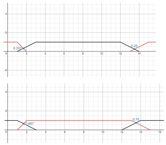
Let us suppose we want to calculate the $Certainty$ value for the constraints ${\pi }_{ij}=(1,2,13,15)$ and ${\pi }_{ij}^{\prime }=(1,3,12,14)$, interpreting each quadruple as a fuzzy number. In this case, by observing Figure 12, we can verify that $Certaint{y}_{ij}(\rho ,{\rho }^{\prime })=min(0.667,0.25)=0.25$.

Figure 12. Visualization of the values obtained for calculating the $Certaint{y}_{ij}(\rho ,{\rho }^{\prime })$ value assuming that the constraints ${\pi }_{ij}$ and ${\pi }_{ij}^{\prime }$ are, respectively, (1,2,13,15) and (1,3,12,14).

In general terms, if we consider the constraints as trapezoidal numbers represented by a quadruple $(\alpha ,\alpha ,\delta ,\delta )$, it is easy to verify that the result will be 1 in cases where both constraints are equal and there is no fuzziness in them, i.e., when all four components of the quadruple coincide. This is also the case when comparing two identical constraints of the type $(\alpha ,\alpha ,\delta ,\delta )$. In fact, the certainty index will measure, in a certain sense, the confidence we have that the distance indicated by the compared constraints coincides. However, this measure is not exempt from counterintuitive examples, as there may be cases where the certainty index is not 1 even though the two constraints are identical, as can be observed in the following example.

Example 7. 

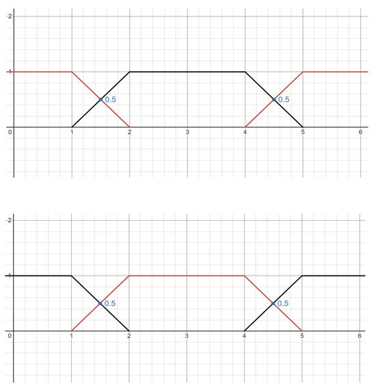
Let us suppose we want to calculate the $Certainty$ value for the constraints ${\pi }_{ij}=(1,2,4,5)$ and ${\pi }_{ij}^{\prime }=(1,2,4,5)$, interpreting each quadruple as a fuzzy number. In this case, by observing Figure 13, we can verify that $Certaint{y}_{ij}(\rho ,{\rho }^{\prime })=min(0.5,0.5)=0.5$.

Figure 13. Visualization of the values obtained for calculating the $Certaint{y}_{ij}(\rho ,{\rho }^{\prime })$ value assuming that the constraints ${\pi }_{ij}$ and ${\pi }_{ij}^{\prime }$ are, respectively, (1,2,4,5) and (1,2,4,5).

Indeed, the certainty index will be 0.5 in all cases where the ${\pi }_{ij}$ and ${\pi }_{ij}^{\prime }$ constraints are equal and trapezoidal. However, depending on the application, an exception could be added to Definition 15 so that in these cases the value would be 1. As we will see in Section 4.2, this will not affect the proof of Theorem 3.

Finally, we understand that the degree of certainty will be given by the maximum of the entailments for all the constraints of the network:

Definition 16. 

At each step of the resolution process in which the clauses $(\varsigma ,\rho )$ and $({\varsigma }^{\prime },{\rho }^{\prime })$ are involved, the following certainty index will be calculated and associated with each resolvent clause $(R(\varsigma ,{\varsigma }^{\prime }),\rho \cap {\rho }^{\prime })$:

$$Certainty(\rho ,{\rho }^{\prime })=\underset{i,j\le n}{max}\{min(Entailment\left({\pi }_{ij}\right|{\rho }^{\prime }),Entailment\left({\pi }_{ij}^{\prime }\right|\rho ))\}$$

It is interesting to note that the fact that this index is calculated for each pair of variables $x_i$ and $x_j$ independently allows for an efficient implementation, so that it can be performed locally while the intersection of constraints between $x_i$ and $x_j$ is being carried out. In other words, a new traversal in the network is not necessary; instead, the values can be stored in a list to then find the maximum of all of them. This means that the computational complexity of each action performed by FTCProlog does not change; that is, it remains as analyzed in [20]. Obtaining this list of certainty indices during the process has another advantage, as it allows for the manipulation of its values according to the interests of the application. It may be, for example, that calculating the average values of the certainty indices is of interest, rather than the maximum. In this case, additional studies would be necessary to verify the correctness of this new index. In Section 4.3, we present a small example in which we have used Definition 16.

4.2. Soundness of the Certainty Measure

In this section, we demonstrate that the proposed measure $Certainty(\rho ,{\rho }^{\prime })$ for calculating the degree of certainty in each deduction in which the clauses $(\varsigma ,\rho )$ and $({\varsigma }^{\prime },{\rho }^{\prime })$ are involved is correct, in the sense that it respects the consistency of FTCLogic.

As we have seen in Section 2.3, the semantics of FTCLogic are based on the measure of necessity given in Definition 11, where $N_{\mathcal{N}}\left(C\right)$ is calculated according to Definition 10.

Furthermore, let us remember that $\mathcal{C}\vDash C$, meaning, a clause C is a logical consequence of a set of FTCClauses $\mathcal{C}$ (according to Definition 12), if for each interpretation $\tau$ that makes ${\gamma }_i$ certain for every $C_i$ and $\gamma$ certain for C , it is fulfilled that $\gamma \ge max{\gamma }_1,...,{\gamma }_n$.

Therefore, what needs to be demonstrated is that, given two FTCClauses $(\varsigma ,\rho )$ and $({\varsigma }^{\prime },{\rho }^{\prime })$, the degree of certainty associated with the resolvent $(R(\varsigma ,{\varsigma }^{\prime }),\rho \cap {\rho }^{\prime })$, proposed in Definition 16, respects this semantic condition. We demonstrate this in Theorem 3, but first we need a definition:

Definition 17. 

We define the local network necessity measure $L{N}_{\mathcal{N}}$ as a function defined by

$L{N}_{\mathcal{N}}((\varsigma ,\rho ),i,j)=inf\{1-{\pi }_{ij}(x_j-x_i),\tau =(\omega ,s),\tau \vDash (\neg \varsigma ,\rho ),s=(x_1,...,x_n)\}$

Lemma 3. 

For each FTCClause $(\varsigma ,\rho )$, it holds that:

$$\underset{i,j\le n}{max}L{N}_{\mathcal{N}}((\varsigma ,\rho ),i,j)=N_{\mathcal{N}}\left((\varsigma ,\rho )\right)$$

Proof. 

This equality is obvious from Definition 2 and Definition 10.    □

Since $L{N}_{\mathcal{N}}((\varsigma ,\rho ),i,j)$ is the infimum of $1-{\pi }_{ij}(x_j-x_i)$ for all assignable values to variables $x_i$ and $x_j$, we call ${\pi }_{ij}^{max}(x_j-x_i)$ the value of ${\pi }_{ij}(x_j-x_i)$ that yields this minimum; that is to say,

$$L{N}_{\mathcal{N}}((\varsigma ,\rho ),i,j)=1-{\pi }_{ij}^{max}(x_j-x_i)$$

Thus, ${\pi }_{ij}^{max}(x_j-x_i)$ is the maximum possibility value among all assignable values to variables $x_i$ and $x_j$.

Lemma 4. 

For any possibility distribution ${\pi }_{ij}^{\prime }$ between two variables $x_i$ and $x_j$, it holds that:

$${\pi }_{ij}^{max}(x_j-x_i)\ge max\underset{n\in DU}{min}({\pi }_{ij}\left(n\right),1-{\pi }_{ij}^{\prime }\left(n\right))$$

Proof. 

Obvious.    □

Now we are in a position to state and prove the following theorem:

Theorem 3. 

Given two FTCClauses $(\varsigma ,\rho )$ and $({\varsigma }^{\prime },{\rho }^{\prime })$, it holds that:

$max(N_{\mathcal{N}}\left((\varsigma ,\rho )\right),N_{\mathcal{N}}\left(({\varsigma }^{\prime },{\rho }^{\prime })\right))\le Certainty(\rho ,{\rho }^{\prime })$

Proof. 

We consider the definition of the network necessity measure for the resolvent clause $(R(\varsigma ,{\varsigma }^{\prime }),\rho \cap {\rho }^{\prime })$:

$$N_{\mathcal{N}}\left((R(\varsigma ,{\varsigma }^{\prime }),\rho \cap {\rho }^{\prime })\right)=inf\{1-{\pi }_S\left(s\right),\tau =(\omega ,s),\tau \vDash (\neg R(\varsigma ,{\varsigma }^{\prime }),\rho \cap {\rho }^{\prime })\}$$

as well as the local network necessity measures for each $i,j\le n$:

$$L{N}_{\mathcal{N}}((R(\varsigma ,{\varsigma }^{\prime }),\rho \cap {\rho }^{\prime }),i,j)=inf\{1-{\pi }_{ij}(x_j-x_i),\tau =(\omega ,s),\tau \vDash (\neg R(\varsigma ,{\varsigma }^{\prime }),\rho \cap {\rho }^{\prime }),s=(x_1,...,x_n)\}.$$

By Lemma 4, it holds that:

$${\pi }_{ij}^{max}(x_j-x_i)\ge max\underset{n}{min}({\pi }_{ij}\left(n\right),1-{\pi }_{ij}^{\prime }\left(n\right))$$

$${\pi }_{ij}^{max}(x_j-x_i)\ge max\underset{n}{min}({\pi }_{ij}^{\prime }\left(n\right),1-{\pi }_{ij}\left(n\right))$$

where ${\pi }_{ij}$ is the possibility distribution between those two variables $x_i$ and $x_j$ in $\rho$, and ${\pi }_{ij}^{\prime }$ is the possibility distribution between those two variables $x_i$ and $x_j$ in ${\rho }^{\prime }$.

Therefore:

$$1-{\pi }_{ij}^{max}(x_j-x_i)\le 1-max\underset{n}{min}({\pi }_{ij}\left(n\right),1-{\pi }_{ij}^{\prime }\left(n\right))=Entailment\left({\pi }_{ij}\right|\rho )$$

$$1-{\pi }_{ij}^{max}(x_j-x_i)\le 1-max\underset{n}{min}({\pi }_{ij}^{\prime }\left(n\right),1-{\pi }_{ij}\left(n\right))=Entailment\left({\pi }_{ij}\right|{\rho }^{\prime })$$

Since $1-{\pi }_{ij}^{max}(x_j-x_i)$ is less than or equal to both values, we can ensure that it is less than or equal to their minimum, namely:

$$L{N}_{\mathcal{N}}((R(\varsigma ,{\varsigma }^{\prime }),\rho \cap {\rho }^{\prime }),i,j)\le min(Entailment\left({\pi }_{ij}\right|{\rho }^{\prime }),Entailment\left({\pi }_{ij}^{\prime }\right|\rho ))$$

or equivalently, for each $i,j\le n$:

$$L{N}_{\mathcal{N}}((R(\varsigma ,{\varsigma }^{\prime }),\rho \cap {\rho }^{\prime }),i,j)\le Certaint{y}_{ij}(\rho ,{\rho }^{\prime })$$

This implies that:

$$\underset{i,j\le n}{max}L{N}_{\mathcal{N}}((R(\varsigma ,{\varsigma }^{\prime }),\rho \cap {\rho }^{\prime }),i,j)\le \underset{i,j\le n}{max}Certaint{y}_{ij}(\rho ,{\rho }^{\prime })$$

By Lemma 3:

$$\underset{i,j\le n}{max}L{N}_{\mathcal{N}}((R(\varsigma ,{\varsigma }^{\prime }),\rho \cap {\rho }^{\prime }),i,j)=N_{\mathcal{N}}\left((R(\varsigma ,{\varsigma }^{\prime }),\rho \cap {\rho }^{\prime })\right)$$

Furthermore, we know from Theorem 1 that:

$$max(N_{\mathcal{N}}\left((\varsigma ,\rho )\right),N_{\mathcal{N}}\left((\varsigma ,{\rho }^{\prime })\right))\le N_{\mathcal{N}}\left((R(\varsigma ,{\varsigma }^{\prime }),\rho \cap {\rho }^{\prime })\right)$$

Summarizing:

$$max(N_{\mathcal{N}}\left((\varsigma ,\rho )\right),N_{\mathcal{N}}\left((\varsigma ,{\rho }^{\prime })\right))\le N_{\mathcal{N}}\left((R(\varsigma ,{\varsigma }^{\prime }),\rho \cap {\rho }^{\prime })\right)\le \underset{i,j\le n}{max}Certaint{y}_{ij}(\rho ,{\rho }^{\prime })$$

That is:

$$max(N_{\mathcal{N}}\left((\varsigma ,\rho )\right),N_{\mathcal{N}}\left((\varsigma ,{\rho }^{\prime })\right))\le Certainty(\rho ,{\rho }^{\prime })$$

which is what we wanted to prove.

   □

We can observe that, as mentioned in Section 4.1, since $Certainty(\rho ,{\rho }^{\prime })$ is an upper bound whose maximum value is 1, assigning an exceptional certainty index of 1 in situations like Example 7 does not affect the proof.

4.3. Study of the Certainty Index through an Example

In this section, we present a small example of the use of FTCProlog where the use of the certainty measure makes sense.

Example 8. 

Suppose in a specific online market study, we found it intriguing to examine the correlation between the number of individuals viewing a product within the first few hours after its publication on the web and the moment when that product reaches its peak visits.

This is compelling in terms of optimizing promotion results for the product, such as maximizing visibility for a potential discount offered some time after its publication.

Specifically, from the analysis of historical data on an online shopping website, a pattern emerges indicating that if, after 12 h following the publication of a product, there are more than a specific number of visits (let us say 1000 visits), then the peak of user visits to that product will occur approximately three days later.

This pattern can be expressed through the following FTCProlog rule:

standard_product(ID) :-

published(ID,PUB),

number_visits_reached(ID,yes,REACH),

peak(ID,PEAK),

time(ID) ;

(PUB,REACH, ’12 hours before’),

(PUB,PEAK, ’approximately 3 days before’).

Next, we create an FTCProgram containing that pattern and the facts corresponding to eight products. By making a query as simple as

c:standard_product(ID).

we can determine all those products whose temporal constraints match the pattern’s completely consistently (that is, the degree of possibility in the network is 1). What we are interested in in this example is analyzing the degree of certainty returned by FTCProlog for each of these products.

The full program can be found in Appendix C. The process of obtaining results using this program can be consulted in Appendix D. We summarize these results in Table 1.

Table 1. Summary of results from Example 8.

NAME	PUB → REACH	>1000 Visits	PUB → PEAK	Matches Pattern	Certainty
prod1	‘12 h before’	yes	‘approximately 3 days before’	yes	1
prod2	(12,12,12,12) h	yes	(0,2,4,6) days	yes	1
prod3	‘approximately 12 h before’	yes	(0,2,4,6) days	yes	0.5
prod4	(9,11,13,15) h	yes	(1,2,4,5) days	yes	0.36486
prod5	(1,2,20,30) h	yes	(1,2,4,5) days	yes	0.47945205
prod6	(1,2,20,30) h	yes	(2,2.5,3,3.5) days	yes	0
prod7	(10,11,12,13) h	yes	(5,6,7,8) days	no	-
prod8	(12,12,12,12) h	no	(0,2,4,6) days	no	-

As we already discussed in Section 4.1, the certainty index is only calculated for predicates that match the pattern with a degree of possibility of 1. What this index measures is the extent to which the temporal restrictions intersecting in the resolution process resemble each other. That is, it measures how similar the network associated with the pattern (or rule) is to the network linking the predicates or facts that are part of the program.

We must keep in mind that in certain applications, this measure would not be useful. There are situations where the temporal constraints between facts are much more precise than those of the pattern (being completely sound), and this is considered an advantage in deductions. In fact, the new constraints obtained as the intersection of the original constraints between the same variables could be considered as a contribution of information, in the sense that it reduces the uncertainty in the time elapsed between certain events.

In the case of the example at hand, what matters is that the temporal constraints are as similar as possible. In that sense, products  prod1  and   prod2  meet this expectation to the fullest, since the constraints from publication time to visit count (PUB to REACH) and from publication time to peak (PUB to PEAK) are exactly the same as those of the pattern. In the case of  prod1, they are expressed using the pseudo-natural language allowed in FTCProlog, while in  prod2, they are expressed with the explicit constraints to which those sentences are translated. For this reason, the certainty measure in the deduction is 1. We should note that this is also due to the fact that one of the constraints is not a fuzzy measure but precise. As we saw in Section 4.1, two identical fuzzy numbers could be evaluated with a certainty index different from 1.

In deductions where the product   prod3  is a standard product, the certainty index decreases to 0.5 because the visit count is not performed exactly at 12 h from publication, but approximately at 12 h after it was published.

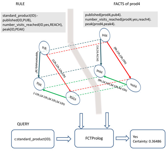
More interesting are the certainty indices obtained for products prod4 and prod5 . In this case, we observe that the PUB-to-PEAK constraint is the same. On the other hand, the comparison between the PUB-to-REACH constraint of each of these products with the corresponding constraint in the pattern necessarily returns 0 in both cases, as the pattern’s constraint is non-fuzzy. This means that the difference in the certainty index of  prod4  and  prod5  is due to a constraint that is not explicitly provided in the FTCProgram, which is the one relating the visit count (REACH) to the peak visits (PEAK). That is, the maximum value obtained in Definition 16 occurs when comparing the constraint between REACH and PEAK of the pattern with the same constraint in each of the products. This constraint, both in the pattern and in the eight products, is initialized to the universal constraint. However, at each step of the resolution process, the networks associated with each clause are minimized. This causes the values for the REACH-to-PEAK constraint to change, both in the pattern and in products prod4 and prod5.

The value associated with this constraint can be obtained by minimizing the network corresponding to each product. This minimization can be performed with a simple query, as reflected in Appendix E. Specifically, it can be observed that in the pattern, the REACH-to-PEAK constraint takes the value  (−12h, 1d 12h, 3d 12h, 5d 12h), in  prod4  the value would be  (9h, 1d 11h, 3d 13h, 4d 15h), and in  prod5  it would be  (−6h, 1d 4h, 3d 22h, 4d 23h). As we can see, the value of the constraint in  prod5  is closer to that of the pattern, which results in a higher certainty index.

In conclusion, we can affirm that this index is useful for comparing the similarity between temporal constraints among the occurrence of different events, but not in isolation, but rather taking into account the complete temporal context. This is because the resolution process incorporates FTCNs and step-by-step minimization processes.

In Figure 14, the deduction process applied to  prod4  is visualized. In the image, temporal constraints that are compared between the network associated with the rule and the one associated with prod4 are shown in similar colors.

Figure 14. Deduction process applied to prod4.

In the case of product  prod6, what happens is that, although its network is consistent with that of the pattern, the values of the constraints deviate enough for the certainty index to be 0.

Finally, products  prod7  and  prod8  do not appear as deductions; in the first case, due to inconsistency in the temporal constraints compared to those of the pattern, and in the second because the visit count does not reach 1000.

5. Discussion and Conclusions

In this work, we introduce FTCProlog, a language similar to Prolog but capable of handling fuzzy temporal constraints among variables. FTCProlog is a modified version of PROLogic. Both FTCProlog and PROLogic are based on FCTLogic, a logical model with two fundamental characteristics:

• Reasoning is complete and sound.
• Treatment of time is efficient.

The properties of soundness and completeness are demonstrated in the definition of FTCLogic, while efficient time management, including implicit common-sense temporal reasoning, is attributed to the incorporation of FTCNs (Fuzzy Temporal Constraint Networks) to manipulate time.

In FTCLogic, clauses consist of a pair comprising a clause in the classical sense and an FTCN that relates the temporal variables appearing in the former. At each step of resolution, the fuzzy intersection between the constraints relating the same variables in the two FTCClauses involved in the process is calculated, ensuring that only consistent networks ultimately form part of a deduction.

As a novelty compared to PROLogic, FTCProlog introduces the computation of a certainty index for each consistent deduction made. This certainty index measures the degree to which the intersected temporal constraints resemble each other. In other words, it quantifies how similar an FTCN associated with a logic rule is to the FTCNs associated with each of the facts involved in the refutation process.

This measure may be of interest in applications requiring the comparison of a temporal pattern with real observations among the same events. In this work, we have defined this certainty index, demonstrated its soundness with respect to the semantics of FTCLogic, and illustrated its utility with a small example.

Moreover, FTCProlog provides a language similar to natural language for expressing fuzzy temporal constraints among variables. This language, already incorporated in PROLogic, has been redefined, and we present its grammar in the form of an appendix. The Alex and Happy tools have been utilized for translating from this language to numerical temporal constraints. The entire tool is implemented in Haskell and can be found at the link in reference [40].

Appendix A.1. Program Syntax

<cons> [:- <ant1>, <ant2>, <ant3>, ..., <antN>]

[; [(<originNode>, <date>)],

constr1,

...

constrM].

constrX can be given as a fuzzy number or as a relation:

constrX =

(<nodeX1>,<nodeX2>,(<double>,<double>,<double>,<double>),

<unit>)

| (<nodeX1>,<nodeX2>,relation)

<unit> can be one of the following words: ‘seconds ’,‘ minutes’, ‘days ’,‘ weeks’, ‘months ’, or ‘years’.

A relation specifies a constraint using pseudo-natural language. PROLogic uses a parser to convert the relations into an equivalent fuzzy number.

<originNode> indicates the name of a node that is associated with <date>.

<date> can be a fuzzy date or an absolute date:

<date> = (<dateISO1>,<dateISO2>,<dateISO3>,<dateISO4>)

| <dateISO>

<dateISO> indicates a date in ISO 8601 format, i.e., YYYY-MM-DDTHH:MM.

If no origin node is specified, PROLogic assigns an unnamed origin node by default, dated 0:00 on January 1 of year 1.

It is possible to include comments in two different ways:

• Single-line comments. Start with % and continue until the end of the line.
  %Single-line comment
• Multi-line comments. Start with /* and end with */.
  /* Multi-
  line
  comment. */

Appendix A.2. Command and Query Syntax

<command> [-<opt1> -<opt2> ... -<optN>]

          [<arg1> <arg2> ... <argM>]

          [: <goal> [; <FTCN>]].

<optX> is a letter that corresponds to an option.

<argY> is an argument.

<goal> is <atom1>, <atom2>, ..., <atomN>

<FTCN> is described as specified in the previous section.

• Load a program

Use:

load <program_file>.

Description:

Load a PROLogic program from a file.

• Make a query

Use:

c [-d|-h|-i] [node1 node2..nodeN] : <goal> [; <FTCN>].

Description:

Normal query of a goal. If no specific nodes are indicated, all will be displayed. If nodes are indicated, only the temporal constraints between them will be written. By default, infinite constraints are omitted. If the goal FTCN is omitted, the universal network will be used by default. That is, an empty FTCN.

Options:

-d: Defuzzified constraints.

-h: Hide the FTCN in the answer.

-i: This shows the infinite constraints.

We can attain another answer, if any, with the n command.

Use:

n [-d|-h|-i] [node1 node2..nodeN].

Description:

Go to the next result of those obtained in the last query.

Options:

-d: Defuzzified constraints.

-h: Hide the FTCN in the answer.

-i: This shows the infinite constraints.

The command last allows us to obtain information about the last answer obtained.

Use:

last [-d|-h|-i] [node1 node2 .. nodeN].

Description:

Returns the current result.

Options:

-d: Defuzzified constraints.

-h: Hide the FTCN in the answer.

-i: This shows the infinite constraints.

• Basic information regarding networks

Commands that allow additional information about the network associated with the last response to be obtained.

firsts tells us which nodes occurred before all the others. There may be several.

Use:

firsts.

Description:

Returns the nodes that represent the initial events of the result network. Returns more than one if they occurred at approximately the same time.

lasts returns the end nodes in the network.

Use:

lasts.

Description:

Returns the nodes that represent the final events of the result network. Returns more than one if they occurred at approximately the same time.

The commands pred and succ return all the nodes that precede and succeed the indicated node, respectively.

Use:

pred <node>.

Description:

Returns the nodes that occurred approximately before <node> in the result network.

Use: succ <node>.

Description:

Returns the nodes that occurred approximately after <node> in the result network.

• Network resolution

The commands time and resolv place each node at an absolute time using an origin node:

Use:

time [-d] [<node1>...<nodeN>].

Description:

It returns an absolute time for each node in the answer network, taking into account the origin node of the network, if it exists.

Options:

-d: Defuzzified constraints.

We can indicate any origin node with the resolv command.

Use:

resolv [-d] <origin_node> <time> [<node1>...<nodeN>].

Description:

It returns an absolute time for each node in the answer network, taking into account the <origin_node> argument.

Options:

-d: Defuzzified constraints.

Arguments:

<origin_node>: node from which the network is resolved.

<time>: time assigned to <origin_node> in ISO-8601 format: YYYY-MM-DDTHH:MM:SS.

• Hypothetical queries

The command hypo allows you to determine the compatibility between a certain piece of information and existing information.

Use:

hypo <node1> <relation> <node2>.

Description:

Compare a hypothetical constraint between two nodes and their real constraint, returning the possibility and necessity values of the Possibilistic Logic.

Arguments:

<node1>: Initial node of the constraint.

<relation>: Relation between the nodes, written in a fuzzy temporal language similar to natural language. This is the same language as that permitted in the temporal relations of the programs.

<node2>: Final node of the constraint.

The possibility degree is a measure between 0 and 1. A 0-value indicates that the relation of the query is impossible, while a 1-value indicates that the relation is totally possible. With respect to necessity degree, it measures the certainty of a relation, signifying that a value greater than 0 would imply a possibility of 1, while a possibility value of 0 would imply a necessity of 0. A necessity value of 0 and a possibility of 1 mean that the relation is completely possible but the certainty is unknown. This implies total ignorance.

• Help command

The command help provides information regarding the syntax of all commands, along with their descriptions and the meaning of their options and arguments.

Use:

help <command1> [<command2>...<comamndN>].

Description: Describe how to use the commands and their arguments.

• End session

In order to close the application from the terminal, it is necessary to use the command q .

Use:

q.

Description: The running of the interpreter ends.

References

- Allen, J.F. Maintaining knowledge about temporal intervals. Commun. ACM 1983, 26, 832–843. [Google Scholar] [CrossRef]
- Gammoudi, A.; Hadjali, A.; Yaghlane, B. Fuzz-time: An intelligent system for managing fuzzy temporal information. Int. J. Intell. Comput. Cybern. 2017, 10, 200–222. [Google Scholar] [CrossRef]
- Dubois, D.; Prade, H. Possibility Theory and its Applications: Where Do we Stand? In Handbook Computational Intelligence; Kacprzuk, J., Pedrycz, W., Eds.; Springer: Berlin/Heidelberg, Germany, 2015; pp. 31–60. [Google Scholar]
- Dubois, D.; Lang, J.; Prade, H. Timed Possibilistic Logic. Fundam. Informaticae 1991, 15, 211–234. [Google Scholar] [CrossRef]
- Marín, R.; Cárdenas-Viedma, M.A.; Balsa, M.; Sánchez, J.L. Obtaining Solutions in Fuzzy Constraint Networks. Int. J. Approx. Reason. 1997, 16, 261–288. [Google Scholar] [CrossRef]
- Barro, S.; Marín, R.; Mira, J.; Patón, A.R. A model and a language for the fuzzy representation and handling of time. Fuzzy Sets Syst. 1994, 61, 153–175. [Google Scholar] [CrossRef]
- Marín, R.; Barro, S.; Bosch, A.; Mira, J. Modeling time representation from a fuzzy perspective. Cybernet Syst. 1994, 25, 207–215. [Google Scholar] [CrossRef]
- Campos, M.; Juarez, J.M.; Palma, J.; Marín, R.; Palacios, F. Avian influenza: Temporal modeling of a human transmission case. Expert Syst. Appl. 2011, 38, 8865–8885. [Google Scholar] [CrossRef]
- Augusto, J.C. The logical approach to temporal reasoning. Artif. Rev. 2001, 16, 301–333. [Google Scholar] [CrossRef]
- Lu, Z.; Augusto, J.; Liu, J.; Wang, H.; Aztiria, A. A system to reason about uncertain and dynamic environments. Int. J. Artif. Intell. Tools 2012, 21, 1250023. [Google Scholar] [CrossRef]
- Bresolin, D.; Goranko, V.; Montanari, A.; Sciavicco, G. Propositional interval neighborhood logics: Expressiveness, decidability, and undecidable extensions. Ann. Pure Appl. Log. 2009, 161, 289–304. [Google Scholar] [CrossRef]
- Aguilera, J.P.; Diéguez, M.; Fernández-Duque, D.; McLean, B. Time and Gödel: Fuzzy Temporal Reasoning in PSPACE. In Logic, Language, Information, and Computation; Springer: Cham, Switzerland, 2022. [Google Scholar] [CrossRef]
- Godo, L.; Vila, L. Possibilistic temporal reasoning based on fuzzy temporal constraints. In Proceedings of the IJCAI’95, Montreal, QC, Canada, 20–25 August 1995. [Google Scholar]
- Alsinet, T.; Godo, L. Towards an automated deduction system for First-order possibilistic logic programming with fuzzy constants. Int. J. Intell. Syst. 2002, 17, 887–924. [Google Scholar] [CrossRef]
- Pnueli, A. The temporal logics of programs. In Proceedings of the 18th Annual Symposium on Foundations of Computer Science (FOCS), Providence, RI, USA, 31 October–1 November 1977; pp. 46–57. [Google Scholar]
- Aguado, F.; Cabalar, P.; Pérez, G.; Vidal, C.; Diéguez, M. Temporal logic programs with variables. Theory Pract. Log. Program. 2017, 17, 226–243. [Google Scholar] [CrossRef]
- Cárdenas-Viedma, M.A.; Marín, R. FTCLogic: Fuzzy Temporal Constraint Logic. Fuzzy Set Syst. 2019, 363, 84–112. [Google Scholar] [CrossRef]
- Dubois, D.; Lang, J.; Prade, H. Possibilistic Logic. In Handbook of Logic in Artificial Intelligence and Logic Programming; Gabbay, D.M., Hogger, C.J., Robinson, J.A., Eds.; Oxford University Press: Oxford, UK, 1994; Volume 3, pp. 439–513. [Google Scholar]
- Dubois, D.; Prade, H. Possibilistic logic—An overview. In Handbook of the History of Logic; Volume 9: Siekmann J (vol. ed) Computational Logic; Gabbay, D.M., Woods, J., Eds.; Elsevier, North-Holland: Amsterdam, The Netherlands, 2015; pp. 283–342. [Google Scholar]
- Cárdenas-Viedma, M.A.; Galindo-Navarro, F.M. PROLogic: A Fuzzy Temporal Constraint Prolog. Int. J. Appl. Math. 2019, 32, 677–719. [Google Scholar] [CrossRef]
- Abadi, M.; Manna, Z. Temporal Logic Programming. J. Symb. Comput. 1989, 8, 277–295. [Google Scholar] [CrossRef]
- Hrycej, T. A Temporal extension of Prolog. J. Log. Program. 1993, 15, 113–145. [Google Scholar] [CrossRef][Green Version]
- Sakuragawa, T. Temporal Prolog. In RIMS Conference on Software Science and Engineering; Springer: Berlin/Heidelberg, Germany, 1987. [Google Scholar]
- Orgun, M.A.; Ashcroft, E.A. (Eds.) Tu Van Le, Fuzzy Temporal Prolog. In Intensional Programming I: Based on the Papers at Islip ’95; World Scientific: Singapore, 1996. [Google Scholar]
- Górriz, J.M.; Álvarez–Illán, I.; Álvarez–Marquina, A.; Arco, J.E.; Atzmueller, M.; Ballarini, F.; Barakova, E.; Bologna, G.; Bonomini, P.; Castellanos-Dominguez, G.; et al. Computational approaches to Explainable Artificial Intelligence: Advances in theory, applications and trends. Inf. Fusion 2023, 100, 101945. [Google Scholar] [CrossRef]
- Zheng, Y.; Xu, Z.; Wang, X. The Fusion of Deep Learning and Fuzzy Systems: A State-of-the-Art Survey. IEEE Trans. Fuzzy Syst. 2022, 30, 2783–2799. [Google Scholar] [CrossRef]
- Sun, C.; Vamvoudakis, K.G. Continuous-Time Safe Learning with Temporal Logic Constraints in Adversarial Environments. In Proceedings of the 2020 American Control Conference (ACC), Denver, CO, USA, 1–3 July 2020; pp. 4786–4791. [Google Scholar] [CrossRef]
- Canabal–Juanatey, M.; Alonso–Moral, J.M.; Catala, A.; Bugarín–Diz, A. Enriching interactive explanations with fuzzy temporal constraint networks. Int. J. Approx. Reason. 2024, 171, 109128. [Google Scholar] [CrossRef]
- Kiani, M.; Andreu-Perez, J.; Hagras, H. A Temporal Type-2 Fuzzy System for Time-Dependent Explainable Artificial Intelligence. IEEE Trans. Artif. Intell. 2023, 4, 573–586. [Google Scholar] [CrossRef]
- Cai, B.; Ding, X.; Sun, Z.; Qin, B.; Liu, T.; Wang, B.; Shang, L. Self-Supervised Logic Induction for Explainable Fuzzy Temporal Commonsense Reasoning. In Proceedings of the Thirty-Seventh AAAI Conference on Artificial Intelligence, Washington, DC, USA, 7–14 February 2023; Volume 37. [Google Scholar]
- Yang, Y.; Xiong, S.; Kerce, J.C.; Fekri, F. Temporal Inductive Logic Reasoning. arXiv 2022, arXiv:2206.05051. [Google Scholar] [CrossRef]
- Leeuwenberg, A.; Moens, M.-F. A Survey on Temporal Reasoning for Temporal Information Extraction from Text. J. Artif. Intell. Res. 2019, 66, 341–380. [Google Scholar] [CrossRef]
- Page, M.J.; McKenzie, J.E.; Bossuyt, P.M.; Boutron, I.; Hoffmann, T.C.; Mulrow, C.D.; Shamseer, L.; Tetzlaff, J.M.; Akl, E.A.; Brennan, S.E.; et al. The PRISMA 2020 statement: An updated guideline for reporting systematic reviews. Syst. Rev. 2021, 10, 89. [Google Scholar] [CrossRef] [PubMed]
- University Libraries, 2024, Creating a PRISMA Flow Diagram: PRISMA 2020. Available online: https://guides.lib.unc.edu/prisma (accessed on 6 June 2024).
- Dechter, R.; Meiri, I.; Pearl, J. Temporal constraint networks. Artif. Intell. 1991, 49, 61–65. [Google Scholar] [CrossRef]
- Kaufmann, A.; Gupta, M. Introduction to Fuzzy Arithmetic; Van Nostrand Reinhold: New York, NY, USA, 1985. [Google Scholar]
- García, L.; Portela, A. Transmisibilidad del COVID-19. Revista Española de Salud Pública. 2020. Available online: https://www.sanidad.gob.es/biblioPublic/publicaciones/recursos_propios/resp/revista_cdrom/Suplementos/Pildoras/pildora29_transmisibilidad_covid_19.pdf (accessed on 25 April 2023).
- Apt, K.R.; van Emden, M.H. Contributions to the Theory of Logic Programming. J. ACM 1982, 29, 841–862. [Google Scholar] [CrossRef]
- Galindo-Navarro, F.M.; Cárdenas-Viedma, M.A. PROLogic 2017. Available online: https://webs.um.es/mariancv/PROLogic/PROLogic.exe (accessed on 11 June 2024).
- Galindo-Navarro, F.M.; Cárdenas-Viedma, M.A. FTCProlog 2024. Available online: https://github.com/mariantocv/FTCProlog (accessed on 11 June 2024).
- Marlow, S. Alex: A Lexical Analyser Generator for Haskell. 2015. Available online: https://www.haskell.org/alex/ (accessed on 11 June 2024).
- Marlow, S. Happy: The Parser Generator for Haskell. 2015. Available online: https://www.haskell.org/happy/ (accessed on 11 June 2024).
- Vila, L.; Godo, L. On fuzzy temporal constraint networks. Mathw. Soft Comput. 1994, 1, 315–334. [Google Scholar]
Disclaimer/Publisher’s Note: The statements, opinions and data contained in all publications are solely those of the individual author(s) and contributor(s) and not of MDPI and/or the editor(s). MDPI and/or the editor(s) disclaim responsibility for any injury to people or property resulting from any ideas, methods, instructions or products referred to in the content. |
© 2024 by the author. Licensee MDPI, Basel, Switzerland. This article is an open access article distributed under the terms and conditions of the Creative Commons Attribution (CC BY) license (https://creativecommons.org/licenses/by/4.0/).