Enhanced Kepler Optimization Method for Nonlinear Multi-Dimensional Optimal Power Flow

Abstract

Multi-Dimensional Optimal Power Flow (MDOPF) is a fundamental task in power systems engineering aimed at optimizing the operation of electrical networks while considering various constraints such as power generation, transmission, and distribution. The mathematical model of MDOPF involves formulating it as a non-linear, non-convex optimization problem aimed at minimizing specific objective functions while adhering to equality and inequality constraints. The objective function typically includes terms representing the Fuel Cost (FC), Entire Network Losses (ENL), and Entire Emissions (EE), while the constraints encompass power balance equations, generator operating limits, and network constraints, such as line flow limits and voltage limits. This paper presents an innovative Improved Kepler Optimization Technique (IKOT) for solving MDOPF problems. The IKOT builds upon the traditional KOT and incorporates enhanced local escaping mechanisms to overcome local optima traps and improve convergence speed. The mathematical model of the IKOT algorithm involves defining a population of candidate solutions (individuals) represented as vectors in a high-dimensional search space. Each individual corresponds to a potential solution to the MDOPF problem, and the algorithm iteratively refines these solutions to converge towards the optimal solution. The key innovation of the IKOT lies in its enhanced local escaping mechanisms, which enable it to explore the search space more effectively and avoid premature convergence to suboptimal solutions. Experimental results on standard IEEE test systems demonstrate the effectiveness of the proposed IKOT in solving MDOPF problems. The proposed IKOT obtained the FC, EE, and ENL of USD 41,666.963/h, 1.039 Ton/h, and 9.087 MW, respectively, in comparison with the KOT, which achieved USD 41,677.349/h, 1.048 Ton/h, 11.277 MW, respectively. In comparison to the base scenario, the IKOT achieved a reduction percentage of 18.85%, 58.89%, and 64.13%, respectively, for the three scenarios. The IKOT consistently outperformed the original KOT and other state-of-the-art metaheuristic optimization algorithms in terms of solution quality, convergence speed, and robustness.

1. Introduction

In recent years, metaheuristic optimization algorithms have gained prominence for addressing Multi-Dimensional Optimal Power Flow (MDOPF) problems efficiently. MDOPF problem represents a non-convex optimization challenge that is difficult to tackle computationally. It seeks for lowering generation costs, decreasing losses, enhancing voltage stability, and reducing pollution reduction [1,2]. Through suitable control variable setting adjustments, MDOPF aims at optimizing the values of the pre-determined objective functions while maintaining compliance with the equality and inequality restrictions of the power system grids [3]. Reducing fuel costs is the most prevalent objective function in power systems. Nevertheless, secure, eco-friendly, and economical operations are crucial for strengthening the power system efficiency and technical considerations. With myriads of constraints, variables, and objective functions, MDOPF can commonly be non-linear and hard to solve.

Multiple extensive study works have been published in the past decades in an attempt to solve the MDOPF problem with traditional optimization approaches such as quadratic programming [4], semi-definite programming [5], nonlinear programming [6], gradient-based method [7], linear programming [8], sequential unconstrained minimization technique [9], Newton’s method [10,11], and interior point [12]. Compared to traditional methods, meta-heuristic algorithms have many advantages, including their ability to find nearly optimal solutions and ease of implementation. However, they contain random elements and are computationally expensive. The metaheuristic’s exploration and exploitation capabilities need to be reflected in order to guarantee effective global optimization and quick convergence. Therefore, it is critical to consider these aspects while considering the best method of action for a given issue.

Utilized across diverse engineering disciplines, the applications of contemporary evolutionary optimization algorithms have been effectively drawn for several renewable energy and power system tasks. In modeling of solar cells, an improved Archimedes Optimization Algorithm [13], dwarf mongoose [14], and Modified Rime-Ice Growth optimizer [15] have been performed for determining the accurate parameters of solar cells considering their different equivalent circuits. In addition, in the optimization of wind turbine, using a binary artificial bee colony algorithm with multi-dimensional updates [16], a binary artificial algae algorithm [17], and modified differential evolution algorithm [18] has been illustrated for wind turbine placement. Moreover, particle swarm optimization has been developed for designing an optimum wind farm layout with active control of turbine yaws [19], and wind power intermittency was demonstrated in [20] via genetic algorithm optimization. Further successful applications in this field include optimizing energy conversion [21], refining operational scheduling, demand side management [22], renewable energies integration [23], and power system optimization [24,25,26].

Moreover, in [27], the load frequency control (LFC) issue was discussed in a standalone micro-grid using a wild horse optimizer-assisted intelligent fuzzy tilt integral derivative with filter—one plus integral (FTIDF-(1 + I)) controller. The proposed system was applied on the IEEE 39-bus system, including solar PV, wind turbine, and diesel generator units. In [28], an autonomous diesel-wind microgrid was illustrated with a PID frequency controller and an integral-type sliding mode control (I-SMC) for effective load frequency control (LFC). Utilizing the artificial gorilla troops optimizer (GTO) for controller parameter tuning, the results showed minimal frequency deviations, faster settling times, and reduced integral errors compared to other methods. To address parameter uncertainty, vague loading behavior, and nonlinearities in interconnected power systems (IPS), a fractional order PID (FOPID) controller for automatic generation control in a two-area reheat thermal IPS was manifested in [29]. The controller parameters were optimized using the Artificial Gorilla Troops optimizer (GTO) with practical nonlinearities such as generation rate constraints and generation dead band.

Recently, several different optimization algorithms and enhanced versions have been applied to solve a wide range of challenging MDOPF problems. The application and its aiming within their respective domain are manifested in Table 1.

Table 1. The application and its aiming within their respective domain.

Algorithm	Application	Advantage	Disadvantage
A modified Rao-2 algorithm [30]	IEEE 30 and IEEE 118 MDOPF	The FC function with and without the renewable energy sources	The Entire Network Losses (ENL) and the Emissions (EE) have not been taken into consideration
krill herd algorithm (KHA) [31]	26-bus and IEEE 57-bus MDOPF	FC, ENL, and voltage deviation functions	EE has not taken into consideration
Opposition-based learning whale optimization algorithm [32]	IEEE 30 MDOPF	FC function	The large system and other objectives have not been considered
A biogeography-based optimizer [33]	IEEE 30-bus and IEEE 57-bus MDOPF		The FC function has been treated as quadratic not sinusoidal
An adaptive multi-team perturbation-guiding JAYA [34]	The IEEE 30 and IEEE 118 of the MDOPF	FC and ENL functions	The EE have not been taken into consideration
A differential-based harmony search algorithm [35]	The IEEE 57 and IEEE 118 of the MDOPF	FC and ENL functions	The EE have not been taken into consideration
Salp swarm algorithm [36]	Different IEEE systems	FC function	The ENL and EE have not been taken into consideration
Adaptive Differential Evolution [37]	A modified IEEE 30-bus test system	FC, ENL, and EE functions	The large systems have not been considered

Differential evolutionary-based optimization techniques have been established over the past few decades to effectively attain the best solution for complicated MDOPF issues [38]. To address the MDOPF problem with maintaining a balance between the exploration and exploitation search, an emended ABC method has emerged with orthogonal learning in [39] to produce Improved ABC (IABC). The IABC has been implemented on the EEE 30- and 118-bus MDOPF considering FC with valve point; however, the ENL and EE have not been taken into consideration. The best solution for MDOPF problems has been characterized using the TLBO in traditional Alternating Current (AC) power networks [40] and hybridized AC systems with advanced Voltage Source Converters (VSCs) technologies [41], respectively. In order to increase global convergence, pitch adjustment was utilized in place of the evolution algorithm’s operation in hybrid DE and Harmony Search (HS) techniques, which were manifested in [42]. This approach has been applied on different IEEE systems with and FC, the ENL, voltage stability; however, EE has not been taken into consideration

In [43], successive history-based adaptive Differential Evolution (DE) has been evaluated and amalgamated with the static penalty tactic to the MDOPF taking into consideration both equality and inequality limitations. This approach has implemented on the IEEE 30- and 118-bus MDOPF considering FC, the ENL, and EE; however, the FC with valve point has not been taken into consideration. To handle the MDOPF problem, the DE emerged with the grey wolf optimizer (GWO) in [44]. This approach has been implemented on the IEEE 30- and 118-bus MDOPF considering FC, the ENL; however, the EE and FC with valve point have not been taken into consideration.

In [45], the Aquila optimizer solver was merged with the arithmetic optimization algorithm and implemented on IEEE 30- and 118-bus MDOPF considering FC, the ENL and EE; however, the FC with valve point has not been taken into consideration. The gravitational search techniques were combined with PSO in [46] and applied on the IEEE 30- and 118-bus MDOPF considering FC with valve point and the ENL; however, EE has not been taken into consideration. Improved algorithmic exploration has been achieved by integrating a modified Sine–Cosine approach with a Lévy flight [47]. This approach has implemented on the IEEE 30- and 118-bus MDOPF considering FC, the ENL; however, the EE and FC with valve point have not been taken into consideration.

An improved colliding bodies optimization (ICBO) algorithm was manifested in [48] and applied on the IEEE 57- and 118-bus MDOPF considering FC with valve point and the ENL; however, EE has not been taken into consideration. Then, the moth swarm algorithm was combined with the gravitational search algorithm in [49] and applied on IEEE 30-, 57-, and 118-bus MDOPF considering only FC; however, FC with valve point, the ENL, and EE have not been taken into consideration. Gaussian barebones (GB) processes and Quasi-oppositional learning (QOL) emerged with social spider optimization in [50] and were applied on IEEE 30-, 57-, and 118-bus MDOPF considering FC with valve point and the ENL; however, and EE have not been taken into consideration.

1.1. Research Gap

Considerable research has been performed about study in the last few years where a wide range of analytical and metaheuristic methods has been employed to evaluate the MDOPF. Even though these approaches have shown some success, there are still a number of drawbacks. For example, certain algorithms have not been able to achieve a suitable processing time and reliability. The problem formulations in unconstrained optimization can result in the violation of constraints, and the algorithms’ increasing performance in solving the problem is insufficient. Additionally, some of these articles have not included the FC, ENL, and EE. Moreover, most of researchers have neglected the valve point impact which results from sinusoidal formulas because it is hard to implement.

1.2. Novelties and Contributions of the Article

Recently, inspired by Kepler’s equations of planetary motion, Mohamed Abdel-Basset et al. [51] presented a novel physics-based metaheuristic of Kepler Optimization Technique (KOT). In order to strike a balance between exploration and exploitation, KOT represents potential solutions as planets whose locations are arbitrarily changed throughout optimization. The motivation is to improve the original KOT stems from the need to enhance its ability to avoid local minima and thus improve the convergence speed and solution quality. The enhanced version, IKOT, addresses this by incorporating enhanced local escaping mechanisms. First, a powerful exploitation tactic is employed to motivate individuals to search for the best possible solution from their perspectives. Secondly, as the iterations progress and exploitation become more crucial, a configurable parameter is introduced to dynamically adjust the balance between exploration and exploitation, helping the algorithm to escape local minima more effectively. The IKOT is applied on the MDOPF with four objective functions, including FC, FC considering the valve point, ENL, and EE, while the constraints encompass power balance equations, generator operating limits, and network constraints such as line flow limits and voltage limits.

The following are the main benefits that this research indicates:

▪

The traditional KOT was integrated with enhanced local escaping mechanisms to improve convergence speed and solution quality.

▪

The enhancement of the KOT, called the proposed IKOT, was developed as an innovative approach to solving MDOPF problems.

▪

Several objective functions of quadratic FC, FC considering the valve point, ENL, and EE were addressed.

▪

Experimental validations of the IKOT algorithm on two standard IEEE 30- and 57-bus test systems demonstrate its superior performance compared to state-of-the-art algorithms in terms of solution quality, convergence speed, and robustness.

The remainder of article is structured as follows. The MDOPF issue associated with the network and a brief overview of the objective functions are presented mathematically in Section 2. Moreover, Section 3 explains the original KOT and the suggested IKOT. The results and comparison of the case studies are shown in Section 4. In Section 5, conclusions are offered.

2. Problem Formulation

Usually, the purpose of the MDOPF issue is to minimize certain objective functions while fulfil system limitations which can be mathematically modelled as follows:

$$\begin{gathered} {\mathit{Min} \mathit{Obj}}_n=\{N_1(\mathit{l},\mathit{m}),N_2(\mathit{l},\mathit{m})\mathrm{\dots },N_n(\mathit{l},\mathit{m})\} \\ \mathrm{Restricted} \mathrm{by}: \mathit{X}(\mathit{l},\mathit{m})=0 \\ \mathrm{and} \mathit{Y}(\mathit{l},\mathit{m})\le 0 \end{gathered}$$

(1)

where ${\mathit{Obj}}_n$ represents the objective function under consideration. The equality and inequality constrained function can be symbolized as X and Y, respectively, which are functions in the vectors of the state and control variables are determined by l and m.

2.1. Problem Objectives

2.1.1. Fuel Generation Costs (FC)

It can be represented in its quadratic form [52] as follows:

$$\mathit{FC}={\displaystyle \sum _{v=1}^{\mathit{Ngt}}{\mathit{c}}_v+{\mathit{b}}_v.{\mathit{Pg}}_v+}{\mathit{a}}_v{.\mathit{Pg}}_v{ }^2\hspace{0.17em}\hspace{0.17em}\mathsf{\$}/hr$$

(2)

where Pg₁, Pg₂, …, Pg_Ngt illustrates the generators output power in MW; c_v, b_v, and a_v define the generator v cost coefficients.

On the other side, Equation (3) is used to compute the generation FC (USD/h) of thermal generators taking the valve point impact into account. Thus, to obtain the FCs model, the quadratic formula is adjusted sinusoidally and incorporated as follows:

$$\mathit{VpEFC}={\displaystyle \sum _{v=1}^{\mathit{Ngt}}{\mathit{c}}_v+{\mathit{b}}_v\times {\mathit{Pgt}}_v+}{\mathit{a}}_v\times {\mathit{Pgt}}_v{ }^2+\left(\left|{\mathit{e}}_v\times (\mathit{sin}({\mathit{f}}_v\times (\mathit{P}\mathit{g}{t}_v^{\mathit{min}}-Pg{t}_v)))\right|\right)$$

(3)

where e_v and f_v manifest the sinusoidal cost parameters of generator v. $Pg{t}_v^{\min }$ and $Pg{t}_v^{ }$ clarify minimum limit and the output power of each generator v, respectively.

2.1.2. Entire Network Losses (ENL)

The ENL can be formulated as follows [53]:

$$ELN={\displaystyle \sum _{\mathit{v}=1}^{\mathit{Nbs}}{\displaystyle \sum _{\mathit{j}=1}^{\mathit{Nbs}}{\mathit{G}}_{\mathit{vj}}{(\mathit{V}}_v{ }^2{+\mathit{V}}_{\mathit{j}}{ }^2}{-2(\mathit{V}}_v{\mathit{V}}_{\mathit{j}}{\mathit{cos}\mathsf{\theta }}_{\mathit{vj}})}\hspace{1em}MW$$

(4)

where G_vj signifies conductance of each line between bus v and j; V and θ determine the Voltage and phase angle; N_bs illustrates the buses’ number.

2.1.3. Entire Emissions (EE)

Reducing the emissions released by the generating units is the third objective function target, which could be explained as follows [54].

$$\mathit{EE}={\displaystyle \sum _{v=1}^{\mathit{Ngt}}({\omega }_v{\mathit{Pgt}}_v{ }^2+{\mathsf{\beta }}_v{\mathit{Pgt}}_v+{\mathsf{\alpha }}_v})/100+{\mathsf{\zeta }}_v{\mathit{e}}^{{\mathsf{\lambda }}_v{\mathit{Pgt}}_v}\hspace{1em}ton/hr$$

(5)

where ${\omega }_v$, β_v, α_v, and ξ_v characterize the emission coefficients of generator v.

2.2. Equality Constraints

These restrictions are described by the load flow balance Formulas (6) and (7).

$${\mathit{Pg}}_{\mathit{k}}-{\mathit{PLD}}_{\mathit{k}}-{\mathit{V}}_{\mathit{k}}\times {\displaystyle \sum _{\mathit{j}=1}^{\mathit{Nbs}}{\mathit{V}}_{\mathit{j}}\times }{(\mathit{G}}_{\mathit{kj}}{\mathit{cos}\mathsf{\theta }}_{\mathit{ik}}+{\mathit{B}}_{\mathit{kj}}{\mathit{sin}\mathsf{\theta }}_{\mathit{kj}})=0, \mathit{k}=\mathsf{1}:\mathit{Nbs}$$

(6)

$${\mathit{Qgt}}_{\mathit{k}}-{\mathit{QLD}}_{\mathit{k}}+{\mathit{Qc}}_{\mathit{k}}-{\mathit{V}}_{\mathit{k}}{\displaystyle \sum _{\mathit{j}=1}^{\mathit{Nbs}}{\mathit{V}}_{\mathit{j}}}{(\mathit{G}}_{\mathit{kj}}{\mathit{sin}\mathsf{\theta }}_{\mathit{kj}}-{\mathit{B}}_{\mathit{kj}}{\mathit{cos}\mathsf{\theta }}_{\mathit{kj}})=0, \mathit{k}=\mathsf{1}:\mathit{Nbs}$$

(7)

where QLD and PLD signify the reactive and active power demand; Qc₁, Qc₂, …, Qc_Nq illustrate MVAr of switched capacitors/reactors; B_vj demonastrates mutual susceptance between buses v and j

2.3. Inequality Constraints

The following categories apply to the inequality restrictions of the MDOPF problem:

(i)

Generator Constraints

$${\mathit{Pgt}}_{{ }_v}^{\mathit{min}}\le {\mathit{Pgt}}_{{ }_v}\le {\mathit{Pgt}}_{{ }_v}^{\mathit{max}}, \mathit{v}=\mathsf{1}:\mathit{Ngt}$$

(8)

$${\mathit{Vgt}}_{{ }_v}^{\mathit{min}}\le {\mathit{Vgt}}_{{ }_v}\le {\mathit{Vgt}}_{{ }_v}^{\mathit{max}}, \mathit{v}=\mathsf{1}:\mathit{Ngt}$$

(9)

$${\mathit{Qgt}}_{{ }_{\mathit{i}}}^{\mathit{min}}\le {\mathit{Qgt}}_{{ }_{\mathit{i}}}\le {\mathit{Qgt}}_{{ }_{\mathit{i}}}^{\mathit{max}}, \mathit{i}=\mathsf{1}:\mathit{Ngt}$$

(10)

Ngt represents Number of generators; Qgt₁, Qgt₂, …, Qgt_Ngt illustrate generators reactive power in MVAr; Vgt₁, Vgt₂, …, Vgt_Ngt shows the generator voltages

(ii)

Transformer Constraints

$${\mathit{Tapc}}_{\mathit{k}}^{\mathit{min}}\le {\mathit{Tapc}}_{\mathit{k}}\le {\mathit{Tapc}}_{\mathit{k}}^{\mathit{max}}, \mathit{k}=1, 2, \dots , \mathit{Ntapc}$$

(11)

$\mathit{Ntapc}$ illustrates number of tap changing transformers; Tapc₁, Tapc₂, …, Tapc_Ntapc Transformer tap settings

(iii)

Security Constraints

$${\mathit{Qc}}_{\mathit{q}}^{\mathit{max}}\le {\mathit{Qc}}_{\mathit{q}}\le {\mathit{Qc}}_{\mathit{q}}^{\mathit{max}}, \mathit{q}=1, 2, \dots , \mathit{Nq}$$

(12)

$${\mathit{VL}}_v^{\mathit{min}}\le {\mathit{VL}}_v\le {\mathit{VL}}_v^{\mathit{max}}, \mathit{v}=\mathsf{1}:\mathit{NPQ}$$

(13)

$$\left|{\mathit{S}}_u\right|\le {\mathit{S}}_u^{\mathit{max}}, \mathit{u}=1, 2, \dots , \mathit{NF}$$

(14)

where VL_v, …, VL_NPQ manifest the Voltages at load buses; SF₁, …, SF_NF MVA characterize the loadings over transmission lines; Nq, denotes the number of VAr devices, NF illustrates Number of system lines.

3. Proposed IKOT for MDOPF Issue

3.1. Standard KOT

Based on Kepler’s formulas regarding the prediction of the planets position and velocity at a particular moment, KOT is a distinctive metaheuristic version in the category of physics-based inspiration [51]. In KOT, the position of each planet operates as a candidate solution that is arbitrarily adjusted during the optimization procedure in relation to the sun, which represents the best candidate solution.

As a result, during the initialization, a population size of N_p planets is going to be assigned at random in Dim dimensions, reflecting the decision variables of an optimization issue, according to the underlying equation:

$${\overrightarrow{X}}_{i,j}(0)={\overrightarrow{X}}_{j,low}+r_1\times \left({\overrightarrow{X}}_{j,up}-{\overrightarrow{X}}_{j,low}\right),i=1:N_p;j=1:Dim$$

(15)

where X_i,j is a solution vector representing each planet containing the control variables with dimension Dim, while r is a randomized produced integer that ranges from 0 to 1. The initialization of the KOT is executed in a random way like other metaheuristics [55]. The constraints of the optimization process is defined through X_j,low and X_j,up, which are the lower and upper limits of each control variable (j), accordingly.

The velocity of every object is then estimated based on its location respect to the sun. This pattern of motion can be mathematically formulated in Equation (16) [56].

$$V_{{ }_i}(t)=\left\{\begin{array}{cc}{r}_4\times H\times ({\overrightarrow{X}}_a-{\overrightarrow{X}}_i)+\left(1-R_{i-norm}(t)\right)\times F\times {\overrightarrow{U}}_2\times {\overrightarrow{r}}_5(r_3{\overrightarrow{X}}_{i,up}-{\overrightarrow{X}}_{i,low})& if R_{i-norm}(t)>0.5\\ \rho (2r_4{\overrightarrow{X}}_i-{\overrightarrow{X}}_b)-{\rho }^{\ast }({\overrightarrow{X}}_b-{\overrightarrow{X}}_a)+\left(1-R_{i-norm}(t)\right)\times F\times {\overrightarrow{U}}_1\times {\overrightarrow{r}}_5({\overrightarrow{X}}_{i,up}-{\overrightarrow{X}}_{i,low})& Else\end{array}\right.$$

(16)

where,

$$H={\left[\mu (t)\times (Ms+m_i)\left|\frac{2}{R_i(t)+\epsilon }-\frac{1}{a_i(t)+\epsilon }\right|\right]}^{0.5}$$

(17)

$$\rho =\overrightarrow{U}\times (r_3\times (1-r_4)+r_4)\times H$$

(18)

$${\rho }^{\ast }=(1-\overrightarrow{U})\times (r_3\times (1-r_5)+r_5)\times H$$

(19)

where V_i(t) describes the velocity of the i^th object at time t; X_i represents the i^th object position; the symbol → that appears on the head of any variable indicates a vector form; U, U₁, and U₂ tend to be integers that are selected at random from the set of numbers {0, 1}; F is an integer number randomly selected belongs to the set {−1, 1}; r₁, r₂, r₃, r₄, and r₅ are random uniformly distributed values within the bounds of [0, 1]; ε is a tiny number used for avoiding a divide-by-zero mistake; the masses of X_s and X_i are represented by Ms and m_i, respectively; X_a and X_b belong to options drawn at random from the entire population; μ(t) signifies the universal gravitational constant; R_i(t) reflects the distance at any time t between each object X_i and the sun X_s; and a_i denotes the semimajor axis of the object i elliptical orbit at time t, and it is determined by Kepler’s third law, which is described in Equation (20), in the following manner:

$$a_i(t)=r_3\times {\left[T_i{ }^2\times \frac{\mu (t)\times (Ms+m_i)}{4{\pi }^2}\right]}^{\frac{1}{3}}$$

(20)

where T_i illustrates the orbital interval of each i^th object i, which is represented by an absolute value. R_i−norm(t) denotes normalizing the Euclidian distance between X_s and X_i and can be described in the following way [51]:

$$R_{i-norm}(t)=\frac{R_i(t)-R_{\min }(t)}{R_{\max }(t)-R_{\min }(t)}$$

(21)

Objects travel closer in proximity to the sun for a period and then away from it throughout their revolution around the sun. KOT models this behavior in two primary stages: exploitation and exploration. KOT investigates objects distant from the sun in quest for creative solutions while employing solutions closer to the sun more precisely in search of new locations near the finest solutions. In line with the preceding procedures, every object distant from the sun’s location is modified as follows [51]:

$${\overrightarrow{X}}_i(t+1)={\overrightarrow{X}}_i(t)+F\times {\overrightarrow{V}}_i(t)+\left(F{g}_i(t)+\left|r\right|\right)\times \overrightarrow{U}\times ({\overrightarrow{X}}_s(t)-{\overrightarrow{X}}_i(t))$$

(22)

where X_i(t + 1) represents the newly discovered location at time t + 1 of for any planet i, X_s(t) provides the sun position regarding the determined best solution, and F acts as a flag employed to alter the searching directions. Fg_i denotes the attracting gravitation force between the sun X_s and any planet X_i, as follows:

$$F{g}_i(t)=e_i\times \mu (t)\times \frac{(\overrightarrow{M{n}_s}\times {\overrightarrow{mn}}_i)}{{\overrightarrow{Rn}}_i{ }^2+\epsilon }+r_4$$

(23)

where μ and ε symbolizes, respectively, gravitational constant and a tiny small value; e_i is a number between 0 and 1 and represents the eccentricity of an orbiting planet that was introduced to give KOT a stochastic quality; and Mn_s and mn_i signify the normalized values of Ms and m_i, that describe the masses of Xs and Xi, respectively, and are provided by Equations (24) and (25), correspondingly [56]:

$$M{n}_s=r_2\times \frac{fi{t}_s(t)-worst(t)}{{\displaystyle \sum _{k=1}^{N_p}\left(fi{t}_k(t)-worst(t)\right)}}$$

(24)

$$m{n}_i=\frac{fi{t}_i(t)-worst(t)}{{\displaystyle \sum _{k=1}^{N_p}\left(fi{t}_k(t)-worst(t)\right)}}$$

(25)

Also, Rn_i indicates the normalized value of R_i that reflects the Euclidian distance as follows [56]:

$$R{n}_i(t)={‖X_s(t)-X_i(t)‖}_2$$

(26)

where worst(t) denotes the solution option with the highest fitness score. where r₂ is a number chosen at random from 0 to 1 in order to diverge the masses of different planets. μ(t) is a function that, in order to regulate searching precision, exponentially declines with time (t) and is described in the following manner [56]:

$$\mu (t)={\mu }_o\times e^{-\gamma \frac{t}{T_{\max }}}$$

(27)

where γ denotes a constant, μ_o represents the starting value, t has become the present iteration number, and T_max belongs to the total iterations’ number.

KOT is going to concentrate on improving the exploitation operation whenever planets are near the sun and would improve the exploring operator if the sun is far away. To enhance both operators even more, the mathematical representation of this idea may be put into action as seen below [56]:

$${\overrightarrow{X}}_i(t+1)={\overrightarrow{U}}_1\times {\overrightarrow{X}}_i(t)+\left(\frac{{\overrightarrow{X}}_a(t)+{\overrightarrow{X}}_s+{\overrightarrow{X}}_i(t)}{3}+\frac{1}{e^{\left(r\times \left(1+(a_2-1)\times r_4\right)\right)}}\times \left(\frac{{\overrightarrow{X}}_i(t)+{\overrightarrow{X}}_s+{\overrightarrow{X}}_a(t)}{3}-{\overrightarrow{X}}_b(t)\right)\right)\times \left(1-{\overrightarrow{U}}_1\right)$$

(28)

where r denotes a random integer produced using the normal distribution, and a₂ represents a cyclical control parameter which slowly decreases from one to two for T cycles over the course of the optimization procedure, as specified as follows:

$$a_2=-1-1\times (\frac{t}{T_{\max }})$$

(29)

The last phase, elitism, ensures the optimal placements for the planets and the sun by implementing an elitist approach. Equation (30) provides a summary of this process [51]:

$${\overrightarrow{X}}_{i,new}(t+1)=\left\{\begin{array}{cc}{\overrightarrow{X}}_i(t+1)& if \mathrm{f}\left({\overrightarrow{X}}_i(t+1)\right)\le \mathrm{f}\left({\overrightarrow{X}}_i(t)\right)\\ {\overrightarrow{X}}_i(t)& Else\end{array}\right.$$

(30)

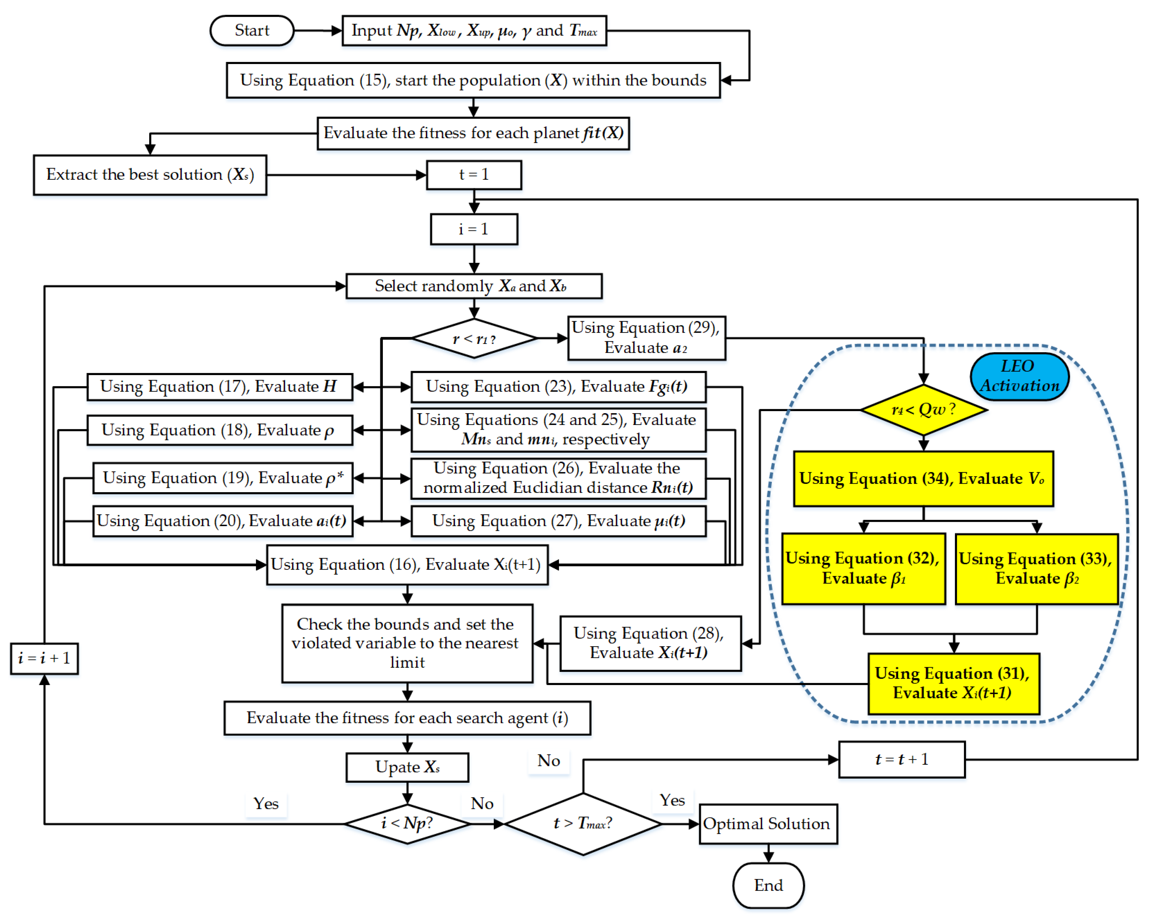
Based on the above-described model, Figure 1 reveals the key steps of the standard KOT.

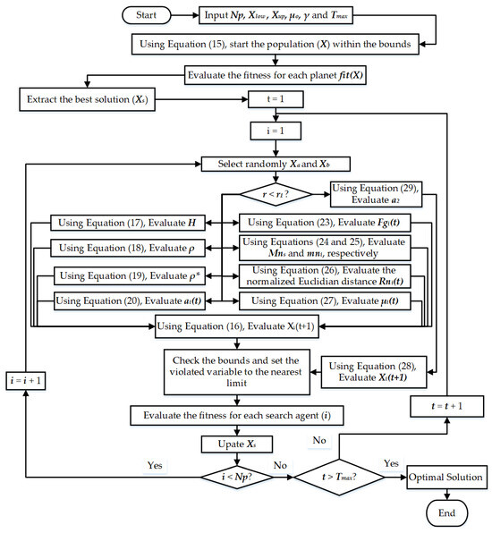
Figure 1. Standard KOT flowchart.

The explanation for Figure 1 is illustrated as follows:

• Initialization:

  ▪

  The algorithm begins by setting the initial population size (Np), which determines the number of candidate solutions to explore concurrently.

  ▪

  It also receives initial values for various parameters, including:

  ▪

  Xiou, Xop, Ho: These likely represent lower and upper bounds for the search space, along with a weighting factor (Ho) that might influence the exploration process.

  ▪

  y and T: The purpose of these variables is not explicitly defined in the figure.

• Fitness Evaluation:

For each solution (represented by a vector) in the initial population, the algorithm calculates its fitness using an unspecified function fit(X). This function likely evaluates how well a particular solution meets the optimization criteria, considering both economic and environmental objectives in a power system scenario.

• Identify the Best Solution:

  ▪

  An initial best solution is chosen, denoted by Xi(t = 1). This might be the solution with the fittest score from the initial population.

  ▪

  A variable i is set to 1, which serves as a counter for iterations.

• Selection and Random Vector Generation:

  ▪

  The algorithm selects two random solutions (Xa and Xb) from the current population.

  ▪

  It then generates a random vector using Equation (29), which is not provided in the image. This random vector might be injected into the population to introduce diversity and prevent stagnation.

• Evaluate Various Components:

  ▪

  Several calculations are performed to assess different aspects of the potential solutions:

  ▪

  Equations (17)–(19): These equations, not shown in the image, likely calculate terms related to the economic or environmental objectives being optimized. For instance, they might determine generation cost, emission levels, or a weighted combination of both.

  ▪

  Equation (23): This equation, also not shown, likely calculates a penalty function (Fg(t)) that might discourage solutions from violating certain constraints.

  ▪

  Equations (24) and (25): These equations, not shown, are likely used to compute quantities related to population diversity (Mn and mni, respectively).

  ▪

  Equation (26): This equation, not shown, calculates the normalized Euclidean distance (Rn(t)) of a solution, which might indicate how far it is from other solutions in the population.

• Update Using Weighted Mean:

Equation (16), not shown in the image, is used to update each solution’s position (Xi(t + 1)) within the search space. This update likely involves a weighted mean based on the fitness (fit(X)) of each solution and potentially other factors.

• Boundary Check:

The updated solution is checked against the lower and upper bounds (Xiou and Xop) using an unspecified function. If any variable in the solution violates the bounds, it is reset to the nearest bound value.

• Fitness Evaluation and Stopping Criteria:

  ▪

  After the update, the fitness of each solution in the population is re-evaluated using fit(X).

  ▪

  The iteration counter (t) is incremented by 1.

  ▪

  Two conditions are checked to determine if the algorithm should stop:

  ▪

  If i < Np (i is less than the population size), the algorithm has not evaluated all solutions in the current population and continues to the next iteration.

  ▪

  If an unspecified stopping criterion is met (likely a maximum number of iterations or a desired level of fitness improvement), the algorithm terminates.

• Update Best Solution:

  ▪

  If the stopping criteria are not met, the algorithm checks if the current best solution (Xi(t)) needs to be updated. It likely compares the fitness of the current best solution with the fittest solution found in the latest iteration.

  ▪

  If a new best solution is found, it is stored as Xi(t + 1).

• Update Xa and Repeat:

  ▪

  The algorithm updates the two selected solutions (Xa and Xb) for the next iteration. How these solutions are updated is not specified in the flowchart.

  ▪

  The process returns to step 4 and repeats until the stopping criteria are met.

• End:

Once the termination condition is satisfied, the algorithm outputs the best solution found (Xi), which represents the optimal operating point for the power system that minimizes the combined generation cost and emission levels.

As shown in Figure 1, the previously described KOT generally depends on two distinct updating strategies to determine and update the locations of the planets. First, Equation (13) represents the exploration strategy, which deals with far objects from the sun, and therefore their locations are updated based on their estimated velocities. Second, Equation (19) represents the exploitation strategy which deals with close objects from the sun. The transfer between both strategies is implemented based on the comparison between two random values {r,r₁}. This transfer mechanism represents approximately an equal way. Therefore, the exploitation strategy will start activation from the beginning of the iteration journey with approximately 50% of the solutions for each iteration. The equal probability of choosing the exploitation strategy from the start of the optimization process leads to premature exploitation. Premature exploitation can cause the algorithm to focus too early on local optima, hindering the thorough exploration of the search space. Effective optimization requires a balance between exploration (searching new areas) and exploitation (refining known good areas). An early and excessive focus on exploitation diminishes the algorithm’s ability to explore the search space adequately, potentially missing better solutions. The lack of a dynamic or adaptive mechanism to balance exploration and exploitation can result in suboptimal optimization performance. The algorithm may converge too quickly to suboptimal solutions due to insufficient exploration of the search space.

Given these issues, the motivation for proposing IKOT likely stems from the need to enhance the balance between exploration and exploitation, prevent premature convergence and improve overall optimization efficiency and effectiveness.

3.2. Proposed IKOT

In order to mitigate this obstacle, a Local Escaping Operator (LEO) was included in the normal KOT to generate an Improved KOT (IKOT), which results in an improved procedure of searching with escaping local optima. The LEO aids in preventing local optima in the program. Employing the associated mathematical model, the KOT approach adjusts the results after each iteration:

$${\overrightarrow{X}}_{i,new}(t+1)=\left\{\begin{array}{cc}{\varphi }_1\left({\beta }_1{\overrightarrow{X}}_s-{\beta }_2{\overrightarrow{X}}_{kv}\right)+\frac{{\sigma }_1{\varphi }_2{\beta }_2}{2}\left({\overrightarrow{X}}_{R1}-{\overrightarrow{X}}_{R2}\right)+{\overrightarrow{X}}_i(t+1)& if r_3<0.5\\ {\varphi }_1\left({\beta }_1{\overrightarrow{X}}_s-{\beta }_2{\overrightarrow{X}}_{kv}\right)+\frac{{\sigma }_1{\varphi }_2{\beta }_2}{2}\left({\overrightarrow{X}}_{R1}-{\overrightarrow{X}}_{R2}\right)+{\overrightarrow{X}}_s& Else\end{array}\right.if r_4<Q_w$$

(31)

where Q_w will be a probability factor which controls the LEO activation. In the range [0, 1], r₃ and r₄ signify randomized values; ϕ₁ and ϕ₂ imply two randomized values attained from a uniform distribution function within the set [−1; 1]; X_R1 and X_R2 are two picked solutions in a random way from the population.

Also, β₁ and β₂ are two randomized number generated via Equations (32) and (33):

$${\beta }_1=2\times r_5\times V_o-\left(V_o-1\right)$$

(32)

$${\beta }_2=r_5\times V_o-\left(V_o-1\right)$$

(33)

$$V_o=\left\{\begin{array}{cc}0& V_1>0.5\\ 1& Else\end{array}\right.$$

(34)

where V₁ denotes an integer generated at random from the range [0, 1].

Figure 2 exhibits the key steps of the proposed IKOT.

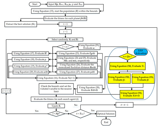
Figure 2. Proposed IKOT flowchart.

3.3. Theoretical Explanation of IKOT

The Local Escaping Operator (LEO) enhances KOT by introducing a mechanism to escape local optima, thereby improving the balance between exploration and exploitation dynamically throughout the optimization process. The LEO helps diversify the search process, especially in the later stages of optimization, preventing premature convergence and improving the overall solution quality.

• Dynamic Balance between Exploration and Exploitation:

  ▪

  In the original KOT, the balance between exploration and exploitation is static, leading to early dominance of exploitation.

  ▪

  IKOT adjusts this balance dynamically by introducing LEO, which activates based on a probability factor Qw, thus providing a more adaptive approach to switching between exploration and exploitation.

2.

Escaping Local Optima:

▪

By incorporating LEO, IKOT can perturb the positions of planets more effectively, helping them escape local optima and explore new regions of the search space.

3.

Key Steps of the Proposed IKOT

• Initialization: Randomly initialize the positions and velocities of planets.
• Exploration Phase: Utilize Equation (22) to update positions based on velocities.
• Exploitation Phase: Apply Equation (28) to refine positions near the best solution.
• Local Escaping Phase: Introduce LEO using Equation (31) to adjust positions and avoid local optima.
• Elitism: Ensure the best solutions are retained for the next iteration using Equation (30).

3.4. The Methodology of IKOT for MDOPF

When addressing the mentioned MDOPF problem, the equality and inequality constraints are taken into account. The Newton-Raphson technique is used to meet the equality requirements describing power flow balancing models. It satisfies the requirements of balance and illustrates how electric grids operate in a steady state. As a result, MATPOWER 6.0 uses the Newton-Raphson technique, which serves as a crucial framework for illustrating three-phase systems [57].

3.4.1. Enhancement of IKOT for Encompassing Operational Constraints of Independent Variables

Equations (8)–(12) manifest the operational boundaries of independent variables that could be adjusted as follows:

$${\mathit{Pg}}_{{ }_{\mathit{k}}}=\left\{\begin{array}{cc}{\mathit{Pgt}}_{{ }_v}^{\mathit{min}}& {\mathit{if} \mathit{Pgt}}_{{ }_v}\le {\mathit{Pgt}}_{\mathit{v}}^{\mathit{min}}\\ {\mathit{Pgt}}_{{ }_v}^{\mathit{max}}& {\mathit{if} \mathit{Pgt}}_{{ }_v}\ge {\mathit{Pgt}}_{{ }_v}^{\mathit{max}}\end{array}\right., \mathit{v}=1, 2, \dots , \mathit{Ngt}$$

(35)

$${\mathit{Vgt}}_{{ }_v}=\left\{\begin{array}{cc}{\mathit{Vgt}}_{{ }_v}^{\mathit{min}}& {\mathit{if} \mathit{Vgt}}_{\mathit{v}}\le {\mathit{Vgt}}_{{ }_v}^{\mathit{min}}\\ {\mathit{Vgt}}_{{ }_v}^{\mathit{max}}& {\mathit{if} \mathit{Vgt}}_{{ }_v}\ge {\mathit{Vgt}}_{\mathit{v}}^{\mathit{max}}\end{array}\right., \mathit{v}=1, 2, \dots , \mathit{Ngt}$$

(36)

$${\mathit{Qgt}}_{{ }_i}=\left\{\begin{array}{cc}{\mathit{Qgt}}_{{ }_i}^{\mathit{min}}& {\mathit{if} \mathit{Qgt}}_{{ }_i}\le {\mathit{Qgt}}_{{ }_i}^{\mathit{min}}\\ {\mathit{Qgt}}_{{ }_i}^{\mathit{max}}& {\mathit{if} \mathit{Qgt}}_{{ }_{\mathit{k}}}\ge {\mathit{Qgt}}_{{ }_i}^{\mathit{max}}\end{array}\right., \mathrm{i}=1, 2, \dots , \mathit{Ngt}$$

(37)

$${\mathit{Tapc}}_k=\left\{\begin{array}{cc}{\mathit{Tapc}}_k^{\mathit{min}}& {\mathit{if} \mathit{Tapc}}_k\le {\mathit{Tapc}}_k^{\mathit{min}}\\ {\mathit{Tapc}}_k^{\mathit{max}}& {\mathit{if} \mathit{Tapc}}_k\ge {\mathit{Tapc}}_k^{\mathit{max}}\end{array}\right., \mathit{k}=1, 2, \dots , \mathit{Ntapc}$$

(38)

$${\mathit{Qc}}_q=\left\{\begin{array}{cc}{\mathit{Qc}}_q^{\mathit{min}}& {\mathit{if} \mathit{Qc}}_q\le {\mathit{Qc}}_q^{\mathit{min}}\\ {\mathit{Qc}}_q^{\mathit{max}}& {\mathit{if} \mathit{Qc}}_q\ge {\mathit{Qc}}_q^{\mathit{max}}\end{array}\right., \mathit{q}=1, 2, \dots , \mathit{Nq}$$

(39)

The factors continue toward their limits as demonstrated, and if any of them exceeds ratings, they are reproduced at random within the relevant bounds.

3.4.2. Enhancement of IKOT for Encompassing Operational Constraints of Dependent Variables

Furthermore, the second category’s limits are penalized and expanded upon by the desired cost objective. As a result, the planet would be eliminated in the following round if its location exceeded any of the relevant restrictions. The considered objective (Obj) may be constructed using these ideas, as demonstrated by Equation (40).

Moreover, the target cost objective expands and penalizes the second category’s limitations. Therefore, if the planet’s location exceeds any of the appropriate constraints, it would be discarded in the next round. Such concepts may be used to construct the contemplated objective (Obj), as shown in Equation (40).

$${\mathit{Obj}=\mathit{Obj}}_{\mathit{j}}{+\mathit{Pe}}_{\mathsf{1}}{\displaystyle \sum _{\mathit{NPQ}}{\Delta \mathit{VL}}_{vv}^{\mathsf{2}}}{+\mathit{Pe}}_{\mathsf{2}}{\displaystyle \sum _{\mathit{Nq}}{\Delta \mathit{Qc}}_{qq}^{\mathsf{2}}}{+\mathit{Pe}}_{\mathsf{3}}{\displaystyle \sum _{\mathit{NF}}{\Delta \mathit{S}}_{uu}^{\mathsf{2}}}, \mathit{j}=\mathsf{1},\mathrm{\dots }\mathit{n}$$

(40)

where ${\Delta \mathit{VL}}_{vv}$, ${\Delta \mathit{Qc}}_{\mathit{qq}}$, and ${\Delta \mathit{S}}_{uu}$ are displayed as:

$${\mathsf{\Delta }\mathit{VL}}_{vv}=\left\{\begin{array}{c}{\mathit{VL}}_v^{\mathit{min}}-{\mathit{VL}}_v{ \hspace{1em}\mathit{if} \mathit{VL}}_v<{\mathit{VL}}_v^{\mathit{min}}\\ {\mathit{VL}}_v^{\mathit{max}}-{\mathit{VL}}_v{ \hspace{1em}\mathit{if} \mathit{VL}}_v>{\mathit{VL}}_v^{\mathit{max}}\end{array}\right.$$

(41)

$${\Delta \mathit{Qc}}_{\mathit{qq}}=\left\{\begin{array}{c}{\mathit{Qc}}_{\mathit{q}}^{\mathit{min}}-{\mathit{Qc}}_q{ \hspace{1em}\mathit{if} \mathit{Qc}}_q<{\mathit{Qc}}_q^{\mathit{min}}\\ {\mathit{Qc}}_q^{\mathit{max}}-{\mathit{Qc}}_q{ \hspace{1em}\mathit{if} \mathit{Qc}}_q>{\mathit{Qc}}_q^{\mathit{max}}\end{array}\right.$$

(42)

$${\Delta \mathit{S}}_{uu}={\mathrm{S}}_u^{\mathit{max}}-{\mathit{S}}_u{ \hspace{1em}\mathit{if} \mathit{S}}_u>{\mathit{S}}_u^{\mathit{max}}$$

(43)

4. Simulation Results

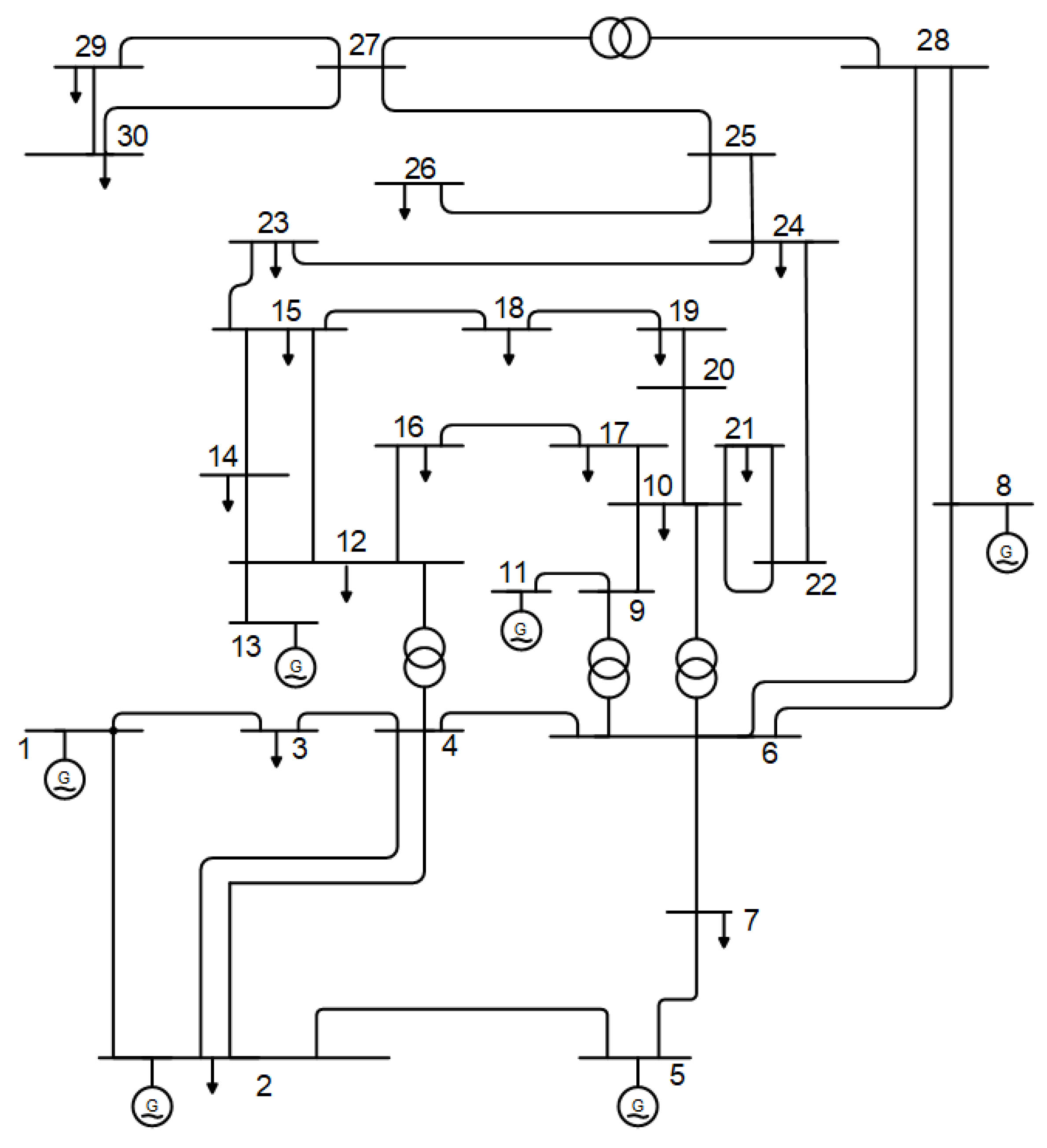
Two test systems of the standard IEEE 30-bus and 57-bus were employed to test the designed IKOT and KOT. Thirty simulation runs were accomplished with a population size of 50 and 300 iterations. As illustrated in Figure 3, the first system consisted of 30 buses, six generators, nine capacitive sources, 41 lines, and four on-load tap changing transformers. The lowest and highest limits for buses, transmission lines, and reactive power generators were drawn from [58]. The generator voltages were 1.1000 (p.u.) at maximum and 0.9500 (p.u.) at minimum. The 30 simulation runs accomplished with the proposed IKOT and KOT for the standard IEEE 57-bus were with a population size of 100 and a maximum number of iterations of 1000. Seven dedicated generators and 57 buses are used in this system. Additionally, three VAr injection devices were placed at buses 15, 25, and 53, as well as tapping changers on 17 transformers. These devices were surrounded by 30 MVAr. The 10% allowed limits must not be exceeded by the bus voltages or the transformer tap control. All the data for this system came from [57].

Figure 3. IEEE 30-bus schematic diagram [59].

4.1. Results of IEEE 30 Bus System

For the IEEE 30 bus system, four scenarios were considered:

▪

Scenario (Sc.) 1: Minimizing the FC

▪

Sc. 2: Minimizing the FC considering Valve Point Effect (VpEFC)

▪

Sc. 3: Minimizing the EE

▪

Sc. 4: Minimizing the ENL

4.1.1. Applications for Sc. 1

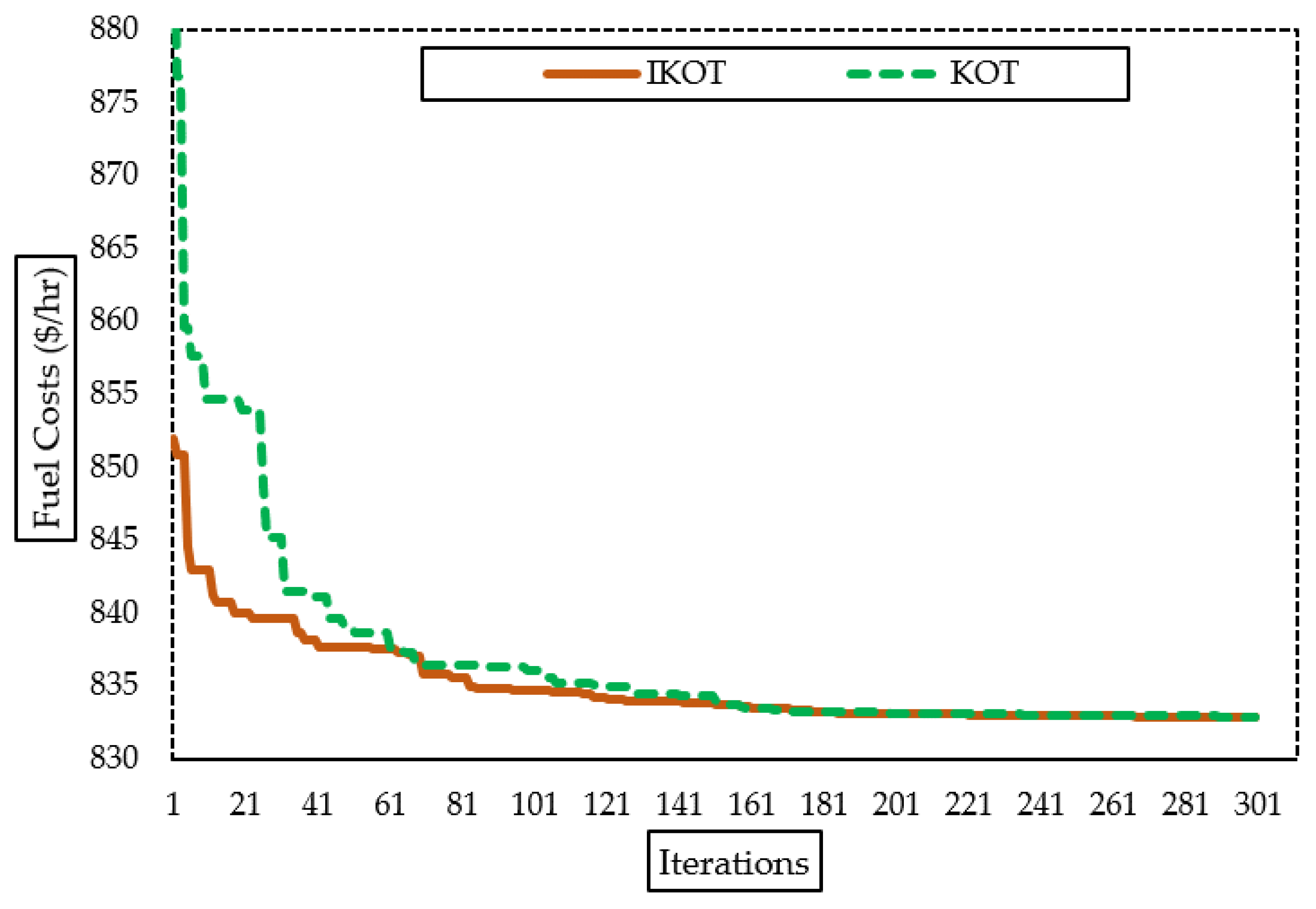
The proposed IKOT and the original KOT were implemented in this scenario. Table 2 presents the optimum outcomes for Sc. 1, comparing the results obtained using the original KOT and the proposed IKOT algorithms. The table provides numerical values for various variables and their corresponding values for the base scenario, KOT, and proposed IKOT. Also, Figure 4 illustrates the corresponding behavior of the IKOT and KOT algorithms in terms of the convergence characteristics for Sc. 1. The results indicate that the IKOT outperformed the KOT in terms of minimizing the FCs. The proposed IKOT performed better than the KOT in terms of minimizing the FCs, where the base scenario, KOT, and the proposed IKOT obtained FC values of USD 901.96/h, 799.09219, and USD 799.08771/h, respectively. This demonstrates the superior performance of the designed IKOT in optimizing the fuel costs. Additionally, the table includes variables related to voltage magnitudes (Vg), tap ratios (Tap), and reactive power generations (Qc) for specific buses, as well as active power generations (Pg) for different generators.

Table 2. Optimum outcomes for Sc. 1 of the IEEE 30-bus system.

Variables	Base	Sc. 1 (FC (USD/h))		Variables	Base	Sc. 1 (FC (USD/h))
		KOT	Proposed IKOT			KOT	Proposed IKOT
Vg 1	1.050	1.0999842	1.0999925	Qc 20	0.000	4.3512481	4.6076627
Vg 2	1.040	1.0875161	1.0874407	Qc 21	0.000	4.9641697	4.9763268
Vg 5	1.010	1.060882	1.0609243	Qc 23	0.000	2.9795945	2.9102967
Vg 8	1.010	1.0686429	1.0689624	Qc 24	0.000	4.9928187	4.9666918
Vg 11	1.050	1.0995761	1.0999881	Qc 29	0.000	2.4323656	2.7008637
Vg 13	1.050	1.0998924	1.0999718	Pg 1	99.240	177.0435773	176.9447176
Tap 6–9	1.078	1.0525044	1.0529859	Pg 2	80.000	48.637559	48.607984
Tap 6–10	1.069	0.9049149	0.901062	Pg 5	50.000	21.292769	21.391957
Tap 4–12	1.032	0.9921532	0.9900401	Pg 8	20.000	21.061161	21.003969
Tap 28–27	1.068	0.9654594	0.9656767	Pg 11	20.000	12.065562	11.975528
Qc 10	0.000	4.9330193	4.999515	Pg 13	20.000	12.018054	12
Qc 12	0.000	4.8984732	4.92006	Cost_Pg	901.9600	799.09219	799.08771
Qc 15	0.000	4.4012584	4.6575448	Losses	5.832400	8.6198222	8.623016
Qc 17	0.000	4.7869863	4.8852291

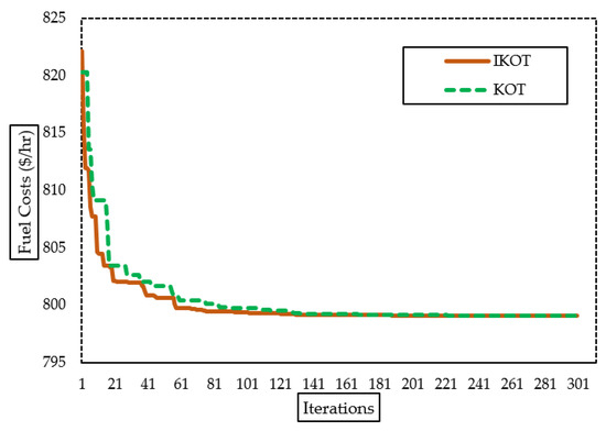
Figure 4. Convergence characteristics of the proposed IKOT and KOT for Sc. 1.

Table 3 presents a comparison of the outcomes obtained from minimizing the FC of Sc. 1 in relation to various other optimization approaches, which are the Black-Hole-Based Optimizing Method (BHBOM) [40], DE versions [52], Symbiotic Organisms Search (SOS) [60], Crow Search Optimization (CSO) [61], Modified CSO (MCSO) [62], Improved Moth-Flame Optimization (IMFO) [63], Developed Grey Wolf Optimization (GWO) [64], Improved Electromagnetism-like Optimization Algorithm (IEOA) [65], Moth Swarm Algorithm (MSA) [66], Ensemble Constraint Handling Technique with DE (ECHT-DE) [67], Evolutionary Algorithm (EA) [68], Grasshopper Optimizer (GO) [69], Genetic Algorithm (GA) [70], Differential Harmony Search Approach (DHSA) [71], Imperialist Competitive Approach (ICA) [72], Teaching-Learning Algorithm (TLA) [73], Novel Bat Optimization (NBO) [74], and adapted GA [75]. As can be illustrated from Table 3, the proposed IKOT obtained the minimum FC among the original KOT and other approaches. This table provides the FC values in USD/h for each method, allowing for a comparative analysis. The proposed IKOT algorithm achieved an FC of USD 799.0824/h, which was the lowest among the listed methods. This demonstrates the effectiveness of the proposed IKOT algorithm in minimizing fuel costs for Sc. 1. Comparing the proposed IKOT with other methods, it was observed that the IMFO achieved an FC of USD 800.3848/h, slightly higher than the proposed IKOT. The KOT algorithm achieved an FC of USD 799.0835/h, which was also close to the result obtained by the proposed IKOT. Several other optimization algorithms are listed in the table, such as TLA, MSA, Adaptive GO, NBO, CSO, GWO, SOS, GO, ICA, JFS, ECHT-DE, Improved EOA, MCSO, DHSA, BHBOA, GA, pbest-DE, Adaptive constraint DE, ensemble constraint handling-DE, self-adaptive penalty-DE, and self-adaptive feasibility-DE. The FC values achieved by these methods range from USD 799.0824/h to USD 802.2966/h. It is evident that the proposed IKOT algorithm performs competitively, as it achieved one of the lowest FC values among the listed methods, indicating its effectiveness in minimizing fuel costs.

Table 3. Comparison for Sc. 1 of the IEEE 30-bus system.

Method	FCs (USD/h)	Method	FCs (USD/h)
Proposed IKOT	799.0824	IMFO [63]	800.3848
KOT	799.0835	SOS [60]	801.5733
MSA [66]	800.5099	ICA [72]	801.843
NBO [74]	799.7516	CSO [61]	799.8266
Developed GWO [64]	800.433	TLA [73]	800.4212
GO [69]	800.9728	Adaptive GO [69]	800.0212
JFS [76]	799.1065	ECHT-DE [67]	800.4148
Improved EOA [65]	799.688	DHSA [40]	802.2966
MCSO [62]	799.3332	GA [70]	802.1962
BHBOA [40]	799.9217	Adaptive constraint DE [77]	800.4113
pbest-DE [52]	800.4115	Self-adaptive penalty-DE [52]	800.4293
Ensemble constraint handling-DE [52]	800.4148	Self-adaptive feasibility-DE [52]	800.4131

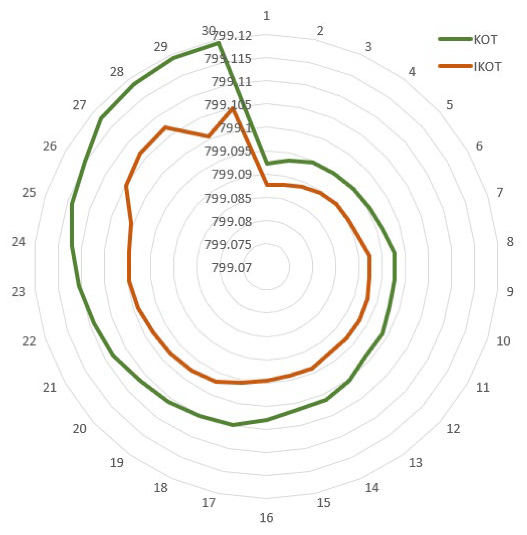
Figure 5 displays the FC outcomes for the 30 different runs for Sc. 1 using the proposed IKOT and KOT. In this regard, Table 4 presents a statistical analysis comparing the KOT algorithm and the proposed IKOT algorithm for Sc. 1 of the IEEE 30-bus system. The table includes numerical values for various statistical measures related to the FCs in USD/h. As shown, the KOT algorithm obtained a best FC of USD 799.09219/h, while the proposed IKOT algorithm achieved a slightly lower best FC of USD 799.08771 /h. This indicates that the proposed IKOT algorithm performs slightly better in terms of obtaining the lowest FC value. Also, the KOT algorithm had a mean FC of USD 799.09907/h, while the proposed IKOT algorithm had a slightly lower mean FC of USD 799.09261/h. Nevertheless, the KOT algorithm had a worst FC of USD 799.10668 /h, whereas the proposed IKOT algorithm achieved a significantly lower worst FC of USD 799.09787/h. This demonstrates the superior performance of the proposed IKOT algorithm in minimizing the worst-case FC. The “STD” column represents the standard deviation of the FC values obtained by each algorithm. The KOT algorithm had a standard deviation of USD 0.0043606/h, while the proposed IKOT algorithm had a lower standard deviation of USD 0.0029867/h. These measures indicate that the proposed IKOT algorithm provides slight improvements in terms of the best FC, mean FC, and worst FC compared to the KOT algorithm. However, the most significant improvement was observed in the standard deviation, where the proposed IKOT algorithm achievesd a substantial reduction of approximately 31.54%. Therefore, the significant reduction in the standard deviation suggests that the proposed IKOT algorithm provides more consistent and stable results across different iterations. The Wilcoxon signed rank test for this scenario is conducted in Table 4 to ensure that the IKOT is really significant compared to the KOT. It can be manifested from the table that the p-value was less than the significance level of 0.05, which means that the IKOT was really significant compared to the KOT.

Figure 5. Thirty runs for FC of Sc. 1 using the proposed IKOT and KOT.

Table 4. Statistical analysis between the KOT and IKOT for Sc. 1 of the IEEE 30-bus system.

Sc. 1 (FC (USD /h))
	KOT	Proposed IKOT
Best	799.09219	799.08771
Mean	799.09907	799.09261
Worst	799.10668	799.09787
STD	0.0043606	0.0029867
p-value	2.7016 × 10−5

4.1.2. VpEFC Minimizing (Sc. 2)

Considering the valve point effect, the IKOT and the KOT were implemented in this scenario to minimize the VpEFC of the IEEE 30-bus system, and Table 5 describes the results which were accomplished. Also, Figure 6 illustrates the corresponding behavior of the proposed IKOT and KOT algorithms in terms of the convergence characteristics for Sc. 2. The proposed IKOT performed better than the KOT in terms of minimizing the VpEFC, where the base scenario, KOT, and the proposed IKOT obtained VpEFC values of USD 901.96/h, 832.87384, and USD 832.81322/h, respectively. As shown, based on the suggested IKOT, the VpEFC was greatly reduced with 7.66% compared to the base scenario.

Table 5. Optimum outcomes for Sc. 2 of the IEEE 30-bus system.

Variables	Base	Sc. 2 (VpEFC (USD/h))		Variables	Base	Sc. 2 (VpEFC (USD/h))
		KOT	Proposed IKOT			KOT	Proposed IKOT
Vg 1	1.050	1.099708	1.099944	Qc 20	0.000	4.687403	5
Vg 2	1.040	1.07985	1.080144	Qc 21	0.000	4.997766	4.847008
Vg 5	1.010	1.054655	1.055772	Qc 23	0.000	3.008146	2.069356
Vg 8	1.010	1.06485	1.063306	Qc 24	0.000	4.325943	4.975328
Vg 11	1.050	1.095728	1.1	Qc 29	0.000	2.873662	3.367333
Vg 13	1.050	1.099848	1.098758	Pg 1	99.240	194.6822	194.6569
Tap 6–9	1.078	1.075327	1.098192	Pg 2	80.000	48.09089	48.25121
Tap 6–10	1.069	0.924231	0.900041	Pg 5	50.000	18.71153	18.61147
Tap 4–12	1.032	1.031119	1.024952	Pg 8	20.000	10	10.00315
Tap 28–27	1.068	0.983189	0.980161	Pg 11	20.000	10.02132	10
Qc 10	0.000	4.238553	2.315208	Pg 13	20.000	12.02861	12.00017
Qc 12	0.000	3.490664	5	VpEFC	901.9600	832.8738	832.8132
Qc 15	0.000	3.288624	4.973036	Losses	5.832400	1.892896	1.979894
Qc 17	0.000	2.893409	4.991811	EE	0.23909633	0.423181	0.423152

Figure 6. Convergence characteristics of IKOT and KOT for Sc. 2.

Moreover, 30 runs were conducted with the proposed IKOT and the original KOT, and the results are depicted in Figure 7. The results illustrate that the proposed IKOT provided VpEFC values which were lower than the original KOT in each run. Additionally, statistical comparisons were developed for both algorithms as manifested in Table 6. In this table, an average VpEFC value of USD 832.86706/h was achieved by the proposed IKOT, while an average VpEFC value of USD 832.94148/h was achieved by the KOT. The Wilcoxon signed rank test for this scenario is conducted in Table 6 to ensure that the IKOT is really significant compared to the KOT. It can be manifested from the table that the p-value was less than the significance level of 0.05, which means that the IKOT was really significant compared to the KOT.

Figure 7. Thirty runs for VpEFC of Sc. 2 using the proposed IKOT and KOT.

Table 6. Statistical analysis between the KOT and IKOT for SC. 2 of the IEEE 30-bus system.

Sc. 2 (VpEFC (USD/h))
	KOT	Proposed IKOT
Best	832.87384	832.81322
Mean	832.94148	832.86706
Worst	832.99096	832.915
STD	0.032684	0.0331139
p-value	1.8215 × 10−5

4.1.3. EE Minimizing (Sc. 3)

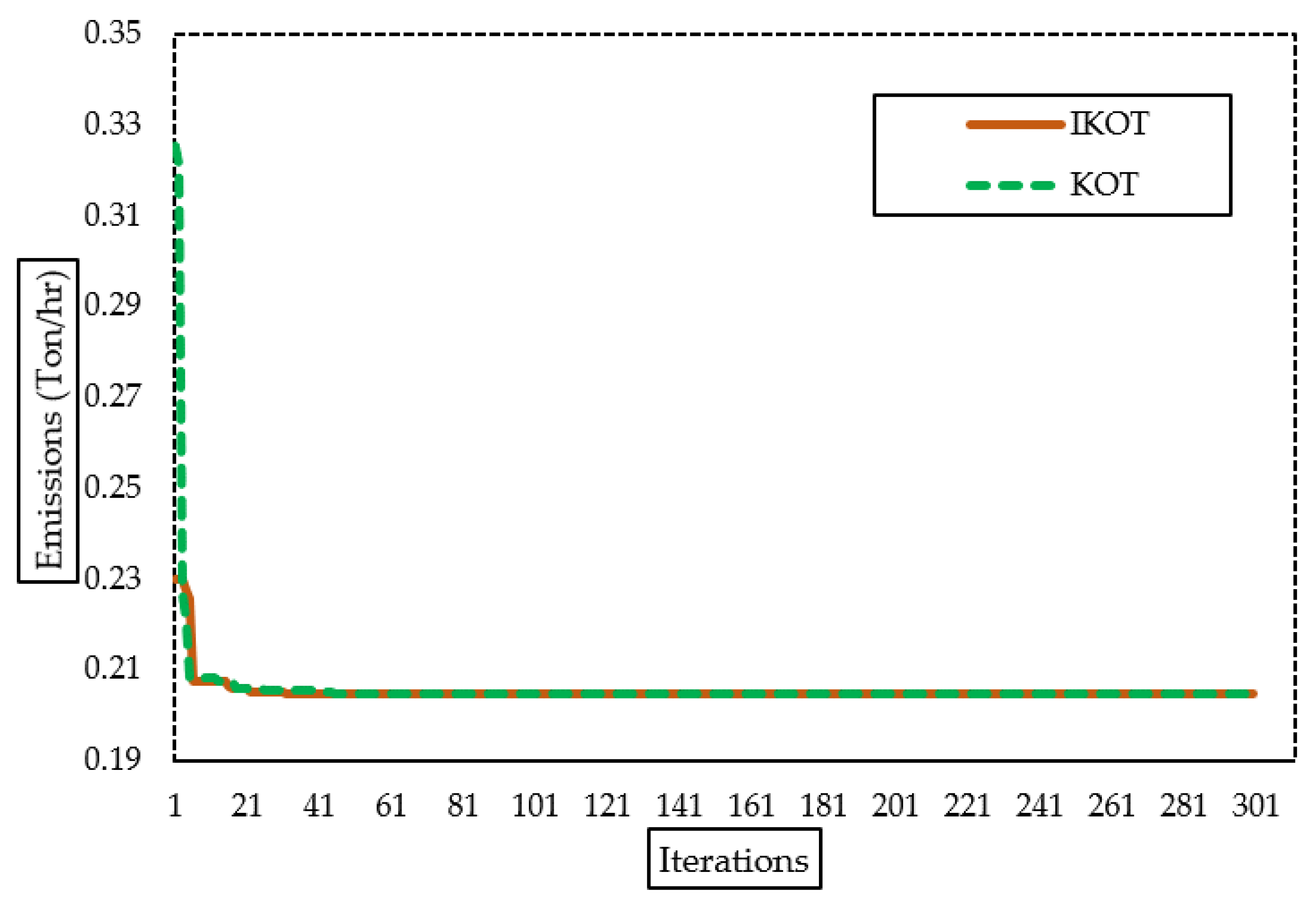
The IKOT and the KOT were implemented in this scenario to minimize the EE of the IEEE 30-bus system, and Table 7 describes the results which were accomplished. The proposed IKOT performed better than the KOT in terms of minimizing the EE, where the base scenario, KOT, and the proposed IKOT obtained EE values of 0.23909633 ton/hr, 0.2046835, and 0.2046825 ton/hr, respectively. Furthermore, Figure 8 exhibits the convergence characteristics of the proposed IKOT and KOT for Sc. 3. In this figure, the proposed IKOT demonstrates how the architecture might lower the total iterations’ number.

Table 7. Optimum outcomes for Sc. 3 of the IEEE 30-bus system.

Variables	Base	Sc. 3 (EE (tonCo2/h))
		KOT	Proposed IKOT
Vg 1	1.050	1.0997405	1.0999696
Vg 2	1.040	1.0949794	1.0964242
Vg 5	1.010	1.0783116	1.0785521
Vg 8	1.010	1.0849409	1.0859791
Vg 11	1.050	1.1	1.0998134
Vg 13	1.050	1.0998329	1.0998638
Tap 6–9	1.078	1.0522669	1.0623459
Tap 6–10	1.069	0.9084085	0.9034771
Tap 4–12	1.032	0.989808	0.9860308
Tap 28–27	1.068	0.9706455	0.9738471
Qc 10	0.000	5	4.9752018
Qc 12	0.000	5	4.9255699
Qc 15	0.000	4.2479758	4.2423648
Qc 17	0.000	5	4.990386
Qc 20	0.000	3.9529735	4.3113485
Qc 21	0.000	5	4.9913136
Qc 23	0.000	2.474512	3.0899092
Qc 24	0.000	4.975469	4.9414417
Qc 29	0.000	2.2314195	2.3724372
Pg 1	99.240	63.87452	63.93249
Pg 2	80.000	67.509343	67.449144
Pg 5	50.000	50	49.999916
Pg 8	20.000	34.999381	34.999844
Pg 11	20.000	30	29.999999
Pg 13	20.000	39.999781	39.999944
Cost_Pg	901.9600	943.6597	943.55787
Losses	5.832400	2.9830268	2.9813334
EE	0.23909633	0.2046835	0.2046825

Figure 8. Convergence characteristics of IKOT and KOT for Sc. 3.

Table 8 presents a comparison of the outcomes obtained from minimizing the EE in relation to various other optimization approaches, which are KHA, Stud KHA [78], GO [69], CSO [62], MCSO [62], modified TLA [79], Adaptive GO [69], Adaptive Real Coded Biogeography-based Technique (ARCBT) [33], MRFA [59], modified TLA [79], and NBA [62]. As can be illustrated from Table 8, the proposed IKOT algorithm achieved the minimum EE among the original KOT algorithm and other approaches. The table includes the algorithm names and their corresponding EE values. Comparing the EE values, we can see that the proposed IKOT algorithm achieved the lowest EE of 0.204681894. Among the other approaches, the closest EE value was obtained by the Adaptive GO algorithm with an EE of 0.20484. The KOT algorithm followed closely with an EE of 0.204682002. Other optimization approaches, such as MRFA, GO, modified TLA, ECHT-DE, ARCBT, JFS, Adaptive constraint DE, pbest-DE, ensemble constraint handling-DE, self-adaptive penalty-DE, and self-adaptive feasibility-DE, also had EE values, but they were higher than the EE achieved by the proposed IKOT algorithm. These results indicate that the proposed IKOT algorithm outperforms the original KOT algorithm and other optimization approaches in terms of minimizing the EE in Scenario 3 of the IEEE 30-bus system. It achieved the lowest EE value compared to the other algorithms, demonstrating its effectiveness in optimizing the trade-off between economic and environmental factors.

Table 8. Comparison for Sc. 3 of the IEEE 30-bus system.

Algorithm	EE	Algorithm	EE
Proposed IKOT	0.204681894	Adaptive GO [69]	0.20484
KOT	0.204682002	MRFA [59]	0.204754
NBO [62]	0.2052063	GO [69]	0.20492
Stud KHA [78]	0.2048	modified TLA [79]	0.20493
MCSO [62]	0.2048911	ECHT-DE [67]	0.20482
KHA [78]	0.2049	ARCBT [33]	0.2048
CSO [62]	0.2051355	JFS [76]	0.204688
pbest-DE [52]	0.2048	Adaptive constraint DE [77]	0.2048
ensemble constraint handling-DE [52]	0.2048	self-adaptive penalty-DE [52]	0.2048
self-adaptive feasibility-DE [52]	0.2048

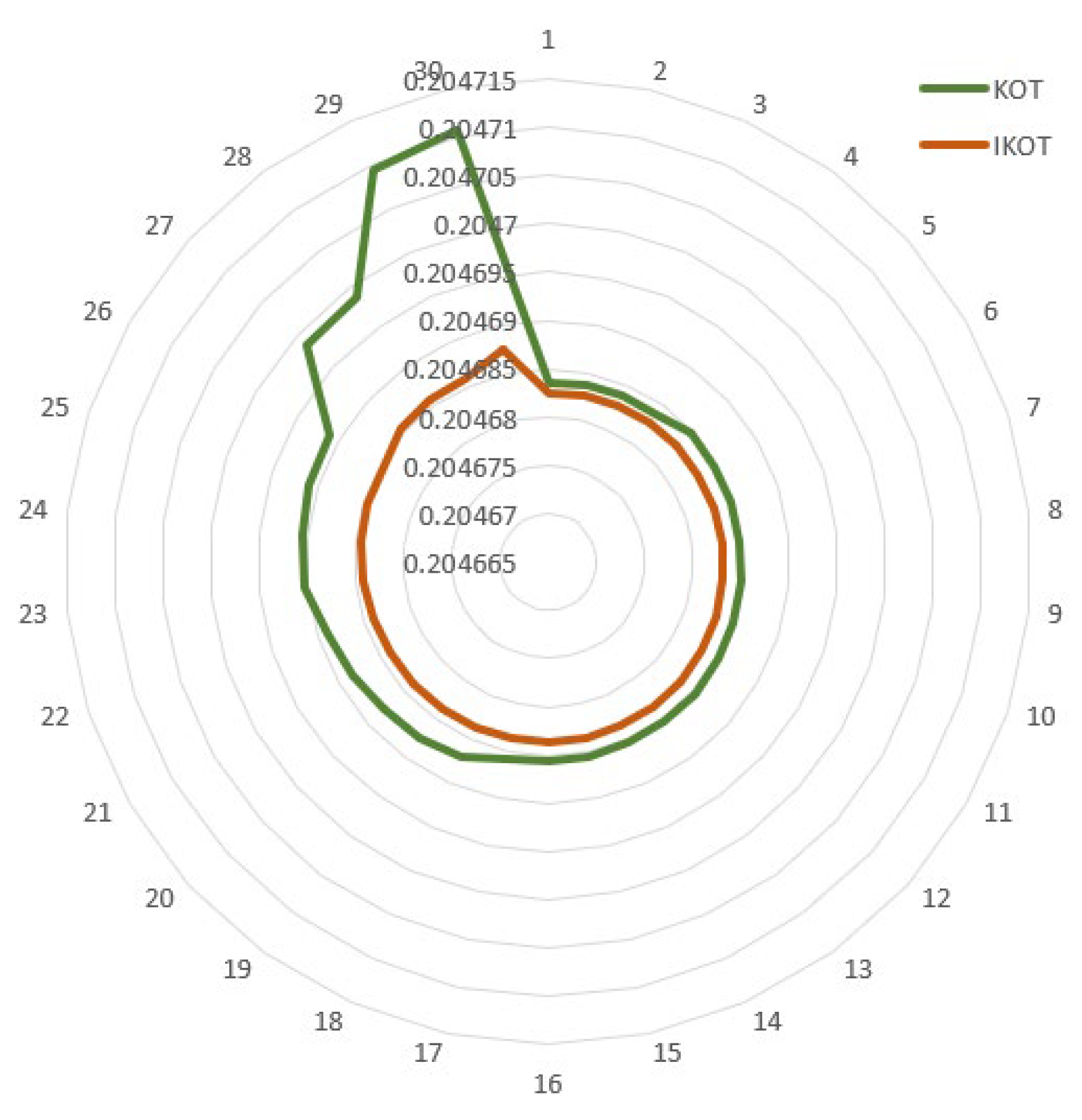
In this scenario, 30 runs were conducted with the proposed IKOT and the original KOT, and the results are depicted in Figure 9. The results illustrate that the proposed IKOT provided EE values which were lower than the original KOT in each run. Additionally, statistical comparisons were developed for both algorithms as manifested in Table 9. In this table, an average EE value of 0.2046832 tonCo₂/h was achieved by the proposed IKOT, while an average EE value of 0.2046853 tonCo₂/h was achieved by the KOT. Similar to the previous analysis, the proposed IKOT algorithm showed slight improvements in the best EE, mean EE, and worst EE compared to the KOT algorithm. However, the most significant improvement was observed in the standard deviation, where the proposed IKOT algorithm achieved a substantial reduction of approximately 64.96%. The Wilcoxon signed rank test for this scenario is conducted in Table 9 to ensure that the IKOT is really significant compared to the KOT. It can be manifested from the table that the p-value was less than the significance level of 0.05 which means that the IKOT was really significant compared to the KOT.

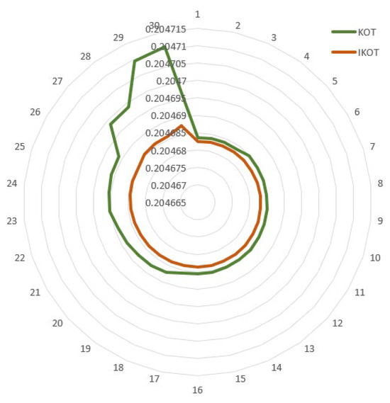
Figure 9. Thirty runs for EE of Sc. 3 using the proposed IKOT and KOT.

Table 9. Statistical analysis between the KOT and IKOT for Sc. 3 of the IEEE 30-bus system.

Sc. 3 (EE (USD/h))
	KOT	Proposed IKOT
Best	0.2046835	0.2046825
Mean	0.2046853	0.2046832
Worst	0.2046878	0.2046838
STD	1.175 × 10−6	4.115 × 10−7
p-value	1.2290 × 10−5

4.1.4. ENL Minimizing (Sc. 4)

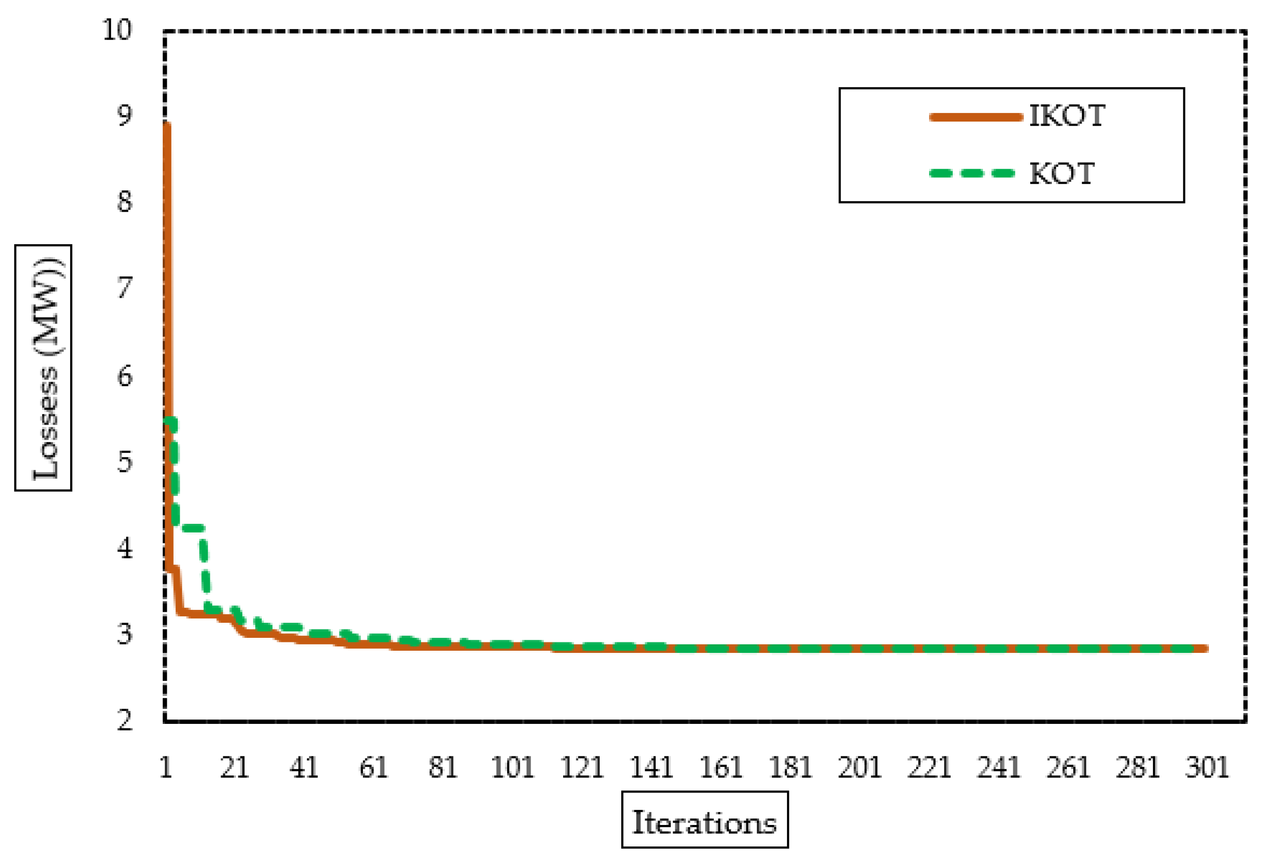
The IKOT and the KOT were implemented in this scenario to minimize the ENL of the IEEE 30-bus system, and Table 10 describes the results which were accomplished. The proposed IKOT performed better than the KOT in terms of minimizing the ENL, where the base scenario, KOT, and the proposed IKOT obtained ENL values of 5.832400 MW, 2.852124, and 2.851063 MW, respectively. Furthermore, Figure 10 exhibits the convergence characteristics of the proposed IKOT and KOT for Sc. 4. In this figure, the proposed IKOT demonstrates how the architecture might lower the total iterations’ number.

Table 10. Optimum outcomes for Sc. 4 of IEEE 30-bus system.

Variables	Base	Sc. 4 (ENL (MW))
		KOT	Proposed IKOT
Vg 1	1.050	1.099979	1.099997
Vg 2	1.040	1.097268	1.097853
Vg 5	1.010	1.07991	1.080156
Vg 8	1.010	1.08744	1.087058
Vg 11	1.050	1.099917	1.099964
Vg 13	1.050	1.099971	1.099975
Tap 6–9	1.078	1.067365	1.069314
Tap 6–10	1.069	0.900134	0.900322
Tap 4–12	1.032	0.987111	0.987483
Tap 28–27	1.068	0.974319	0.974083
Qc 10	0.000	5	4.994113
Qc 12	0.000	4.941765	4.999269
Qc 15	0.000	4.361995	4.690106
Qc 17	0.000	4.91106	4.991473
Qc 20	0.000	4.488789	4.314588
Qc 21	0.000	4.998338	4.99429
Qc 23	0.000	2.723986	2.655286
Qc 24	0.000	4.962214	4.993665
Qc 29	0.000	2.347776	2.305081
Pg 1	99.240	51.27529	51.25339
Pg 2	80.000	79.98773	79.99853
Pg 5	50.000	49.99908	49.99977
Pg 8	20.000	35	34.99976
Pg 11	20.000	29.99779	29.99967
Pg 13	20.000	39.99223	39.99993
FC	901.9600	967.0152	967.0631
ENL	5.832400	2.852124	2.851063
EE	0.23909633	2.612035	2.608253

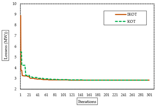
Figure 10. Convergence characteristics of the proposed IKOT and KOT for Sc. 4.

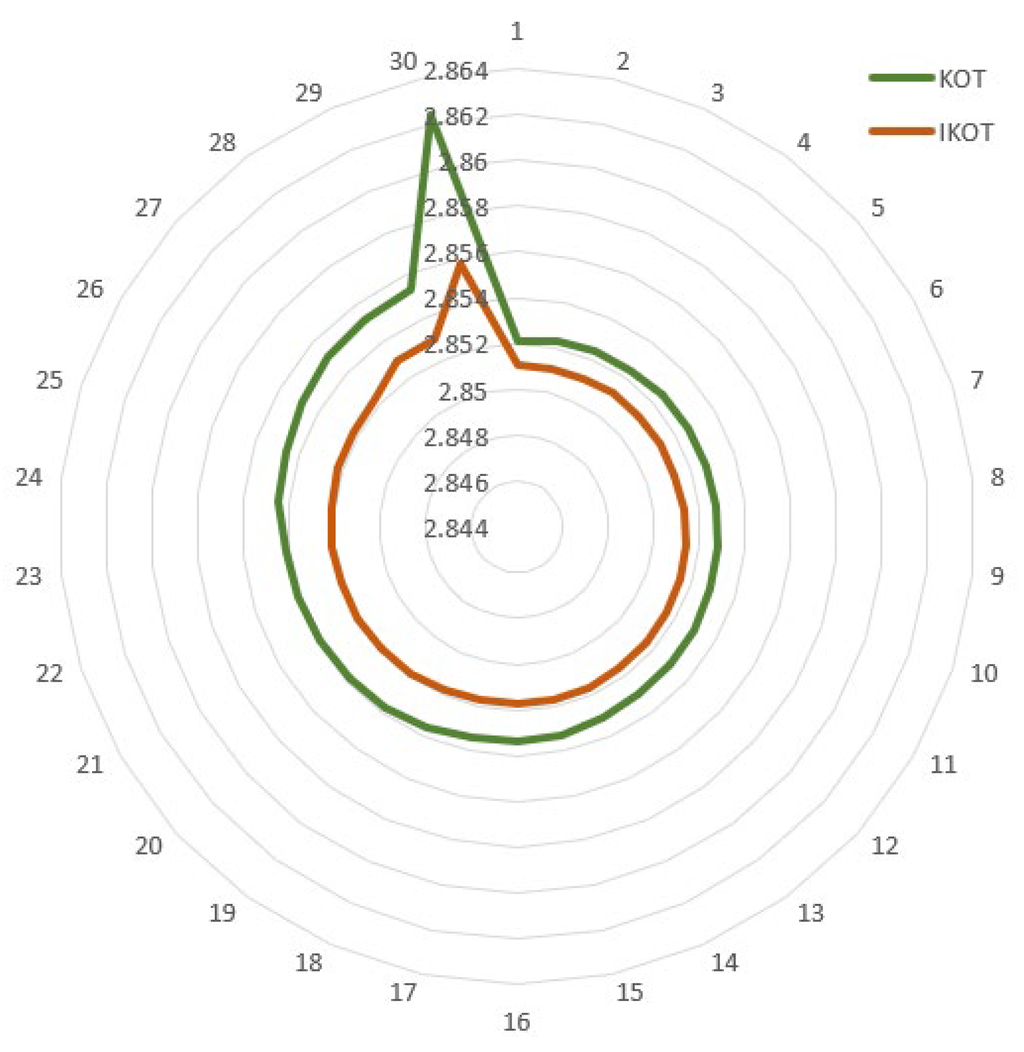
In this scenario, 30 runs were conducted with the proposed IKOT and the original KOT, and the results are depicted in Figure 11. The results illustrate that the proposed IKOT provided ENL values which were lower than the original KOT in each run. Additionally, statistical comparison was developed for both algorithms as manifested in Table 11. In this table, an average ENL value of 2.8514778 MW was achieved by the proposed IKOT, while an average ENL value of 2.8529505 MW was achieved by the KOT. By calculating the improvement percentages, the proposed IKOT algorithm achieved a percentage improvement of 0.0371%, 0.0516%, and 0.0673% compared to the KOT algorithm for the best, mean ENL, and worst ENL. Also, the proposed IKOT algorithm achieved a percentage improvement of (0.0004966 − 0.0002901)/0.0004966 × 100 ≈ 41.65% compared to the KOT algorithm. However, the most significant improvement was observed in the standard deviation, where the proposed IKOT algorithm achieved a substantial reduction of approximately 41.65%. These results indicate that the proposed IKOT algorithm performs slightly better than the KOT algorithm in terms of the ENL measures, with the most notable improvement seen in the standard deviation. The reduced standard deviation suggests that the proposed IKOT algorithm yields more consistent and stable ENL values. The Wilcoxon signed rank test for this scenario is conducted in Table 11 to ensure that the IKOT is really significant compared to the KOT. It can be manifested from the table that the p-value was less than the significance level of 0.05 which means that the IKOT was really significant compared to the KOT.

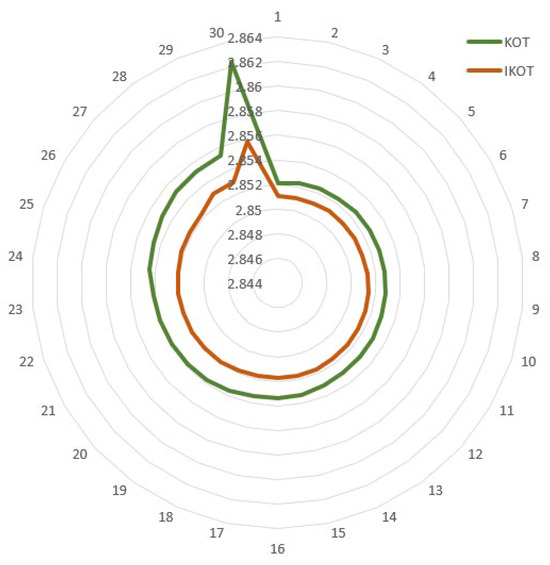
Figure 11. Thirty runs for ENL of Sc. 4 using the proposed IKOT and KOT.

Table 11. Statistical analysis between the KOT and IKOT for Sc. 4 of the IEEE 30-bus system.

Sc. 4 (ENL (USD/h))
	KOT	Proposed IKOT
Best	2.8521238	2.8510628
Mean	2.8529505	2.8514778
Worst	2.8539049	2.8519867
STD	0.0004966	0.0002901
p-value	8.2981 × 10−6

4.2. Results of IEEE 57 Bus System

Three scenarios for this system were examined as follows:

▪

Sc. 5: Minimizing the FC

▪

Sc. 6: Minimizing the EE

▪

Sc. 7: Minimizing the ENL

For this system, the IKOT and the KOT were implemented in three scenarios to minimize the FC, EE, and ENL, and Table 12 describes the results for these scenarios which were accomplished. The table includes the variables and their corresponding values for both algorithms. It also includes the values of different variables such as Vg (generator voltage), Tap (transformer tap ratio), Qc (reactive power injection), and Pg (active power generation) for both algorithms in each scenario. As manifested in this table, the proposed IKOT algorithm outperformed the KOT algorithm in terms of minimizing the FC, minimizing the EE, and maximizing the ENL in Scenarios 5, 6, and 7 of the IEEE 57-bus system. The IKOT algorithm achieved lower values for the FC and EE objectives and a higher value for the ENL objective, demonstrating its effectiveness in optimizing multiple objectives simultaneously.

Table 12. Optimum outcomes obtained via the proposed IKOT and KOT for Scs. 5, 6, and 7 of the IEEE 57-bus system.

Variables	Base	Sc. 5 (FC (USD/h))		Sc. 6 (EE (Ton/h))		Sc. 7 (ENL (MW))
		KOT	IKOT	KOT	IKOT	KOT	IKOT
Vg 1	1.010	1.0528589	1.0490981	1.0512586	1.06	1.0512314	1.0599683
Vg 2	1.010	1.0505598	1.0465119	1.0436187	1.056154	1.0446953	1.0566525
Vg 3	1.010	1.0476581	1.0408582	1.0486027	1.053503	1.0443166	1.06
Vg 6	1.010	1.057303	1.0526739	1.0415265	1.047782	1.0443103	1.06
Vg 8	1.010	1.0594182	1.0598524	1.0495426	1.059955	1.0491184	1.06
Vg 9	1.010	1.0359735	1.0334266	1.0336925	1.03923	1.0273124	1.0412399
Vg 12	1.010	1.0401997	1.0352904	1.0462459	1.044963	1.0349537	1.04861
Tap 4–18	0.970	1.071804	0.9660857	1.1	0.909915	0.9396409	1.0075575
Tap 4–18	0.978	1.0341457	1.0019481	0.9792202	1.00174	1.0477643	0.9752831
Tap 21–20	1.043	1.0415915	1.0145196	0.9813358	0.983893	0.9906537	0.981745
Tap 24–25	1.000	0.9793877	1.0713834	1.0045759	1.087896	1.0067073	1.0542884
Tap 24–25	1.000	1.0593901	0.9450148	1.0764719	1.023525	0.9733652	0.9612857
Tap 24–26	1.043	1.0092304	1.0131516	0.9982919	1.05058	1.0479778	1.014219
Tap 7–29	0.967	0.9564098	0.9497392	0.927779	1.048719	1.0423613	0.9752843
Tap 34–32	0.975	1.0263921	0.9704916	0.9382754	1.048395	0.9909048	0.955498
Tap 11–41	0.955	0.9400717	0.9	1.0131983	0.940488	0.931761	0.937831
Tap 15–45	0.955	0.941064	0.9354061	0.9512305	0.967193	0.9923906	0.9491786
Tap 14–46	0.900	0.952092	0.9248971	1.0823589	0.989219	0.9856068	0.9501329
Tap 10–51	0.930	0.9427316	0.9281249	1.0101604	1.013262	0.9876213	0.9570339
Tap 13–49	0.895	0.9145605	0.9108794	1.00109	0.984496	0.9557236	0.91698
Tap 11–43	0.958	0.9241284	0.9261256	0.975155	0.990354	0.9948324	0.9799994
Tap 40–56	0.958	1.0053302	1.0172206	0.9684819	1.06986	1.0445029	1.044269
Tap 39–57	0.980	0.9809085	0.9625971	1.0140668	1.035583	1.017883	1.0478388
Tap 9–55	0.940	0.969669	0.9431252	1.0408582	1.079417	1.0507726	0.9765349
Qc 18	10.000	19.588645	16.833535	24.273151	4.044177	9.6662115	19.372384
Qc 25	5.900	15.822386	13.469753	17.154082	16.24767	13.372862	9.937805
Qc 53	6.300	14.669189	10.478507	2.9450366	14.62376	13.726467	12.958884
Pg 1	478.635	142.3647278	144.2304109	328.6973467	336.0299972	185.9860937	165.2769025
Pg 2	0.000	90.880229	89.614122	100	100	29.03113	35.605772
Pg 3	40.000	44.99367	44.216258	140	139.9991	116.90941	140
Pg 6	0.000	78.532235	70.349615	100	100	94.841309	90.058955
Pg 8	450.000	455.1729	460.81591	249.12933	259.8651	326.41964	320.08809
Pg 9	0.000	91.893133	94.588597	100	99.9803	98.460077	100
Pg 12	310.000	361.90877	361.80614	257.74474	238.2888	410	409.75317
FC (USD/h)	51345	41677.349	41666.963	48615.481	48775.07	43765.77	44634.796
EE (Ton/h)	2.528	2.6117209	3.1226054	1.0484899	1.039368	1.5410877	2.683034
ENL (MW)	27.8346	14.945665	14.821043	24.771408	23.36324	10.847654	9.9828921

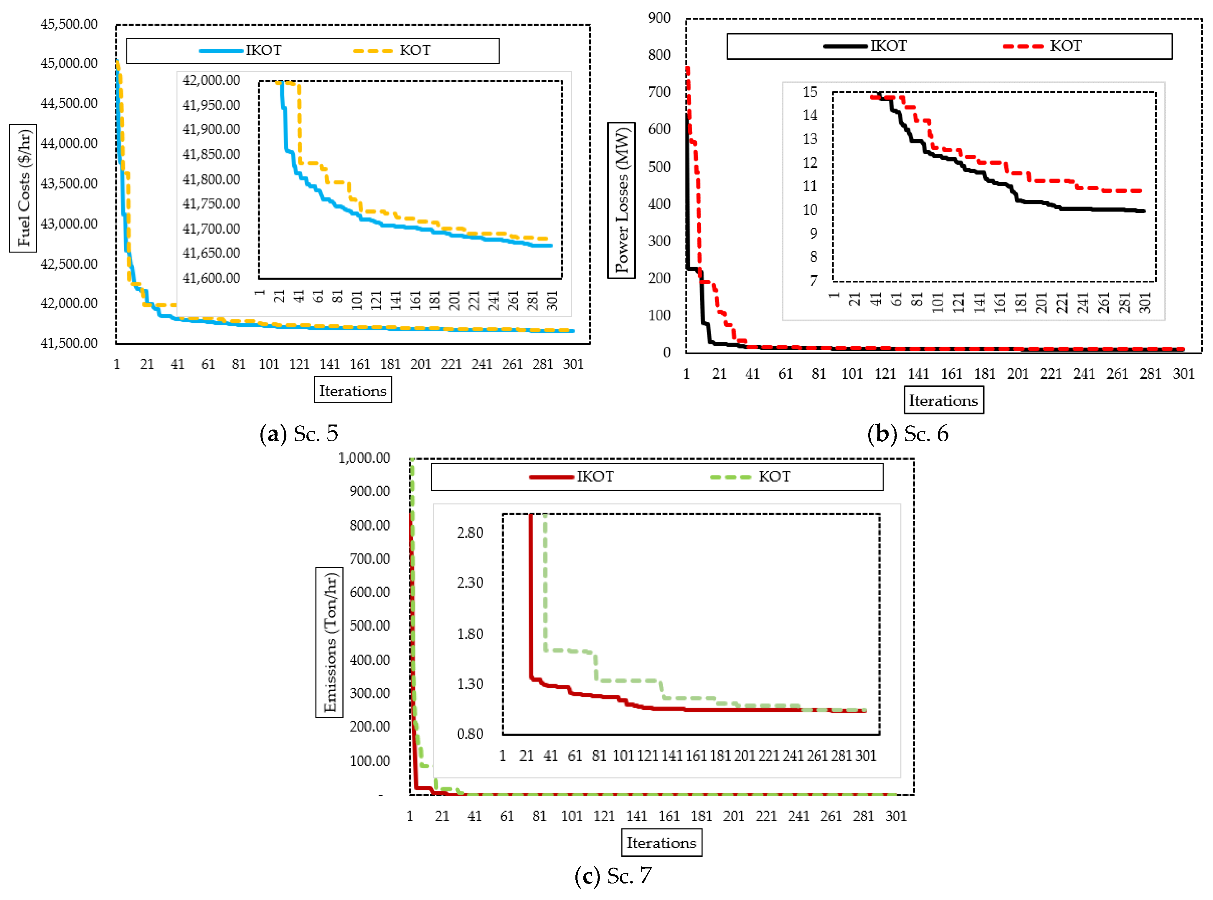
For Sc. 5, the proposed IKOT performed better than the KOT in terms of minimizing the FC, where the base scenario, KOT, and the proposed IKOT obtained FC values of USD 51,345/h, 41,677.349, and USD 41,666.963/h, respectively. In comparison to the base scenario, the IKOT in this scenario achieved a reduction percentage of 18.85%.

Additionally, for Sc. 6, the proposed IKOT performed better than the KOT in terms of minimizing the EE, where the base scenario, KOT, and the proposed IKOT obtained EE values of 2.528 Ton/h, 1.0484899, and 1.0393678 Ton/h, respectively. In comparison to the base scenario, the IKOT in this scenario achieved a reduction percentage of 58.89%.

Moreover, for Sc. 7, the proposed IKOT performed better than the KOT in terms of minimizing the ENL, where the base scenario, KOT, and the proposed IKOT obtained ENL values of 27.8346 MW, 11.277533, and 9.0879067 MW, respectively. In comparison to the base scenario, the IKOT in this scenario achieved a reduction percentage of 64.13%.

Furthermore, Figure 12 exhibits the convergence characteristics of the proposed IKOT and KOT for the three scenarios. In this figure, the proposed IKOT demonstrates how the architecture might lower the total iterations’ number.

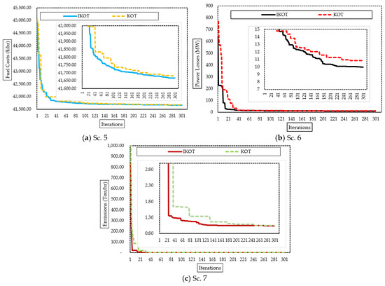
Figure 12. Convergence characteristics of the proposed IKOT and KOT for Scs. 5, 6, and 7 of the IEEE 57-bus system.

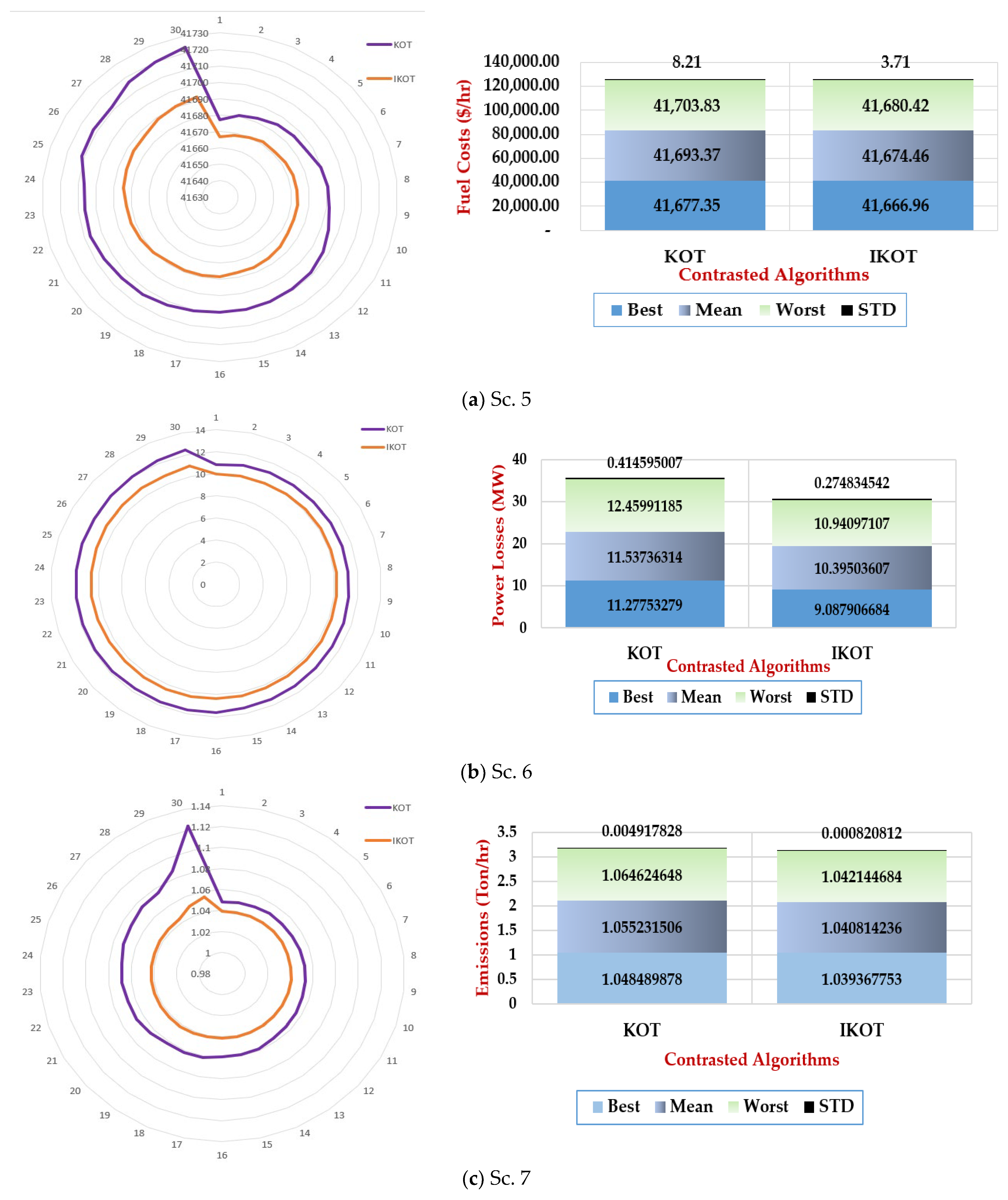
Moreover, in this scenario, 30 runs were conducted for the three scenarios of the IEEE 57-bus system using the proposed IKOT and the original KOT, and the results are depicted in Figure 13. The results illustrate that the proposed IKOT provided the FC, EE, and ENL which were lower than the original KOT in each run. Additionally, statistical comparison was developed for both algorithms as manifested in the mentioned figure. In this figure, the average values of USD 41,674.464/h, 1.0408142 Ton/h, and 10.395036 MW were achieved by the proposed IKOT for the FC, EE, and ENL, respectively, while the average values of USD 41,693.369/h, 1.0552315 Ton/h, and 11.537363MW were achieved by the KOT. Moreover, standard deviation (STD) values of 3.7127467, 0.0008208, and 0.2748345 were achieved by the proposed IKOT for the FC, EE, and ENL, respectively, while the average values of 8.2112032, 0.0049178, and 0.414595 were achieved by the KOT.

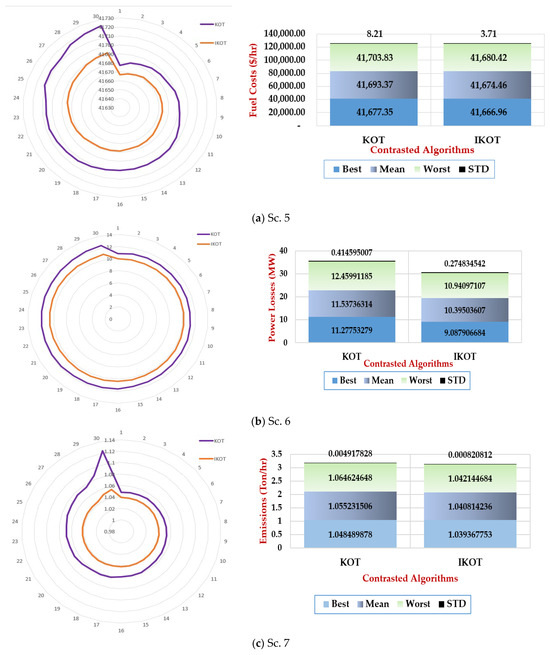
Figure 13. Thirty runs for FC, EE, and ENL of Scs. 6, 7, and 8 using the proposed IKOT and KOT.

The Wilcoxon signed rank test for the three scenarios of the IEEE 57 are conducted in Table 13 to ensure that the IKOT is really significant compared to the KOT. It can be manifested from Table 13 that the p-value for the three scenarios was less than the significance level of 0.05, which means that the IKOT was really significant compared to the KOT.

Table 13. The Wilcoxon signed rank test for the three scenarios of the IEEE 57.

	Sc. 5 (FC (USD/h))	Sc. 6 (ENL (MW))	Sc. 7 (EE (Ton/h))
p-value	3.7896 × 10−6	2.5631 × 10−6	1.7344 × 10−6

4.3. Implications

The findings of this study have several important implications for the operation and planning of power systems:

• Reduced operational costs: By achieving lower fuel costs, the IKOT algorithm can potentially lead to significant cost savings for power generation companies. These savings can be passed on to consumers or reinvested in improving the power grid infrastructure.
• Improved environmental performance: By minimizing emissions, IKOT can contribute to reducing the environmental impact of power generation. This is becoming increasingly important as concerns about climate change grow.
• Reduced energy losses: Lower energy losses translate to a more efficient power grid. This can help to improve the overall reliability of the power system and reduce the need for additional power generation capacity.
• Faster computation times: The faster convergence characteristics of IKOT suggest that it may be computationally more efficient than conventional methods. This can be beneficial for real-time applications where quick solutions are needed.

4.4. Discussion

The results of this study are promising and suggest that the IKOT algorithm has the potential to be a valuable tool for solving OPF problems in power systems. However, some additional discussion points need to be considered:

• Performance on larger systems: The study only investigates the performance of IKOT on the IEEE 30-bus and 57-bus test systems. It is important to evaluate how the algorithm scales to handle much larger power systems encountered in real-world applications.
• Integration with existing systems: Implementing a new optimization algorithm like IKOT may require modifications to existing power system control and management systems. Further research is needed to ensure smooth integration and compatibility.
• Comparison with other algorithms: While the study mentions comparisons with other optimization algorithms, a more comprehensive benchmark including popular methods would provide a clearer picture of IKOT’s relative strengths and weaknesses.
• Practical implementation challenges: The document focuses on the algorithmic aspects of IKOT. Further research is needed to explore the practical challenges of implementing IKOT in real-world power systems, such as data availability, handling uncertainties, and robustness to system disturbances.

5. Conclusions

This paper proposes an innovative approach called the Improved Kepler Optimization Technique (IKOT) to effectively solve the complex optimization problem of the Multi-Objective Optimal Power Flow (MDOPF). The IKOT algorithm was developed by incorporating enhanced local escaping mechanisms that improved the convergence speed and solution quality of the traditional Kepler Optimization Technique (KOT). Additionally, the IKOT algorithm addressed several objective functions, including fuel costs, emission levels, and network losses minimization, making it a versatile solution for power system operation optimization. Experimental validations were conducted on two standard IEEE test systems (30-bus and 57-bus) through seven different scenarios, demonstrating the superior performance of the IKOT algorithm. Compared to state-of-the-art algorithms, the IKOT algorithm exhibited superior solution quality, convergence speed, and robustness. These results highlight the effectiveness and efficiency of the IKOT algorithm in tackling the MDOPF problem. The statistical evidence provided by the results of IKOT’s best, worst, average, and standard deviation underscores its dependability and robustness. Further research is needed to combine the sophisticated IKOT approach variants with various constraint handling techniques to potentially speed up convergence and improve the quality of solutions, especially for large-scale and more complex power systems performance that have numerous and single objective functions to evaluate its performance. Moreover, adjusting the power system parameters that are subjected to uncertainty and variability, such as renewable energy integration and varying load demands, could provide insights into its robustness and flexibility.

References

- Risi, B.-G.; Riganti-Fulginei, F.; Laudani, A. Modern Techniques for the Optimal Power Flow Problem: State of the Art. Energies 2022, 15, 6387. [Google Scholar] [CrossRef]
- Skolfield, J.K.; Escobedo, A.R. Operations research in optimal power flow: A guide to recent and emerging methodologies and applications. Eur. J. Oper. Res. 2022, 300, 387–404. [Google Scholar] [CrossRef]
- Niknam, T.; Narimani, M.R.; Aghaei, J.; Azizipanah-Abarghooee, R. Improved particle swarm optimisation for multi-objective optimal power flow considering the cost, loss, emission and voltage stability index. IET Gener. Transm. Distrib. 2012, 6, 515–527. [Google Scholar] [CrossRef]
- Granelli, G.P.; Montagna, M. Security-constrained economic dispatch using dual quadratic programming. Electr. Power Syst. Res. 2000, 56, 71–80. [Google Scholar] [CrossRef]
- Bai, X.; Wei, H. A semidefinite programming method with graph partitioning technique for optimal power flow problems. Int. J. Electr. Power Energy Syst. 2011, 33, 1309–1314. [Google Scholar] [CrossRef]
- Dommel, H.W.; Tinney, W.F. Optimal Power Flow Solutions. IEEE Trans. Power Appar. Syst. 1968, PAS–87, 1866–1876. [Google Scholar] [CrossRef]
- Lee, K.Y.; Park, Y.M.; Ortiz, J.L. A United Approach to Optimal Real and Reactive Power Dispatch. IEEE Power Eng. Rev. 1985, PER–5, 42–43. [Google Scholar] [CrossRef]
- Zehar, K.; Sayah, S. Optimal power flow with environmental constraint using a fast successive linear programming algorithm: Application to the algerian power system. Energy Convers. Manag. 2008, 49, 3362–3366. [Google Scholar] [CrossRef]
- Rahli, M.; Pirotte, P. Optimal load flow using sequential unconstrained minimization technique (SUMT) method under power transmission losses minimization. Electr. Power Syst. Res. 1999, 52, 61–64. [Google Scholar] [CrossRef]
- Sun, D.I.; Ashley, B.; Brewer, B.; Hughes, A.; Tinney, W.F. Optimal power flow by Newton approach. IEEE Trans. Power Appar. Syst. 1984, PAS-103, 2864–2880. [Google Scholar] [CrossRef]
- Crisan, O.; Mohtadi, M.A. Efficient identification of binding inequality constraints in the optimal power flow Newton approach. IEE Proc. C Gener. Transm. Distrib. 1992, 139, 365–370. [Google Scholar] [CrossRef]
- Wei, H.; Sasaki, H.; Kubokawa, J.; Yokoyama, R. An interior point nonlinear programming for optimal power flow problems with a novel data structure. IEEE Power Eng. Rev. 1997, 17, 134–141. [Google Scholar] [CrossRef]
- Krishnan, H.; Islam, M.S.; Ahmad, M.A.; Rashid, M.I.M. Parameter identification of solar cells using improved Archimedes Optimization Algorithm. Optik 2023, 295, 171465. [Google Scholar] [CrossRef]
- Moustafa, G.; Smaili, I.H.; Almalawi, D.R.; Ginidi, A.R.; Shaheen, A.M.; Elshahed, M.; Mansour, H.S.E. Dwarf Mongoose Optimizer for Optimal Modeling of Solar PV Systems and Parameter Extraction. Electronics 2023, 12, 4990. [Google Scholar] [CrossRef]
- Hakmi, S.H.; Alnami, H.; Moustafa, G.; Ginidi, A.R.; Shaheen, A.M. Modified Rime-Ice Growth Optimizer with Polynomial Differential Learning Operator for Single- and Double-Diode PV Parameter Estimation Problem. Electronics 2024, 13, 1611. [Google Scholar] [CrossRef]
- Hakli, H. The optimization of wind turbine placement using a binary artificial bee colony algorithm with multi-dimensional updates. Electr. Power Syst. Res. 2023, 216, 109094. [Google Scholar] [CrossRef]
- Beşkirli, M.; Koç, İ.; Haklı, H.; Kodaz, H. A new optimization algorithm for solving wind turbine placement problem: Binary artificial algae algorithm. Renew. Energy 2018, 121, 301–308. [Google Scholar] [CrossRef]
- Hakli, H. A new approach for wind turbine placement problem using modified differential evolution algorithm. Turkish J. Electr. Eng. Comput. Sci. 2019, 27, 4659–4672. [Google Scholar] [CrossRef]
- Song, J.; Kim, T.; You, D. Particle swarm optimization of a wind farm layout with active control of turbine yaws. Renew. Energy 2023, 206, 738–747. [Google Scholar] [CrossRef]
- Kim, T.; Song, J.; You, D. Optimization of a wind farm layout to mitigate the wind power intermittency. Appl. Energy 2024, 367, 123383. [Google Scholar] [CrossRef]
- Boryseiko, O.; Laptiev, O.; Perehuda, O.; Ryzhov, A. Optimizing Energy Conversion in a Piezo Disk Using a Controlled Supply of Electrical Load. Axioms 2023, 12, 1074. [Google Scholar] [CrossRef]
- Jasim, A.M.; Jasim, B.H.; Neagu, B.-C.; Alhasnawi, B.N. Efficient Optimization Algorithm-Based Demand-Side Management Program for Smart Grid Residential Load. Axioms 2022, 12, 33. [Google Scholar] [CrossRef]
- Smaili, I.H.; Almalawi, D.R.; Shaheen, A.M.; Mansour, H.S.E. Optimizing PV Sources and Shunt Capacitors for Energy Efficiency Improvement in Distribution Systems Using Subtraction-Average Algorithm. Mathematics 2024, 12, 625. [Google Scholar] [CrossRef]
- Sarhan, S.; Shaheen, A.; El-Sehiemy, R.; Gafar, M. An Augmented Social Network Search Algorithm for Optimal Reactive Power Dispatch Problem. Mathematics 2023, 11, 1236. [Google Scholar] [CrossRef]
- Mahmoud, M.M.; Atia, B.S.; Esmail, Y.M.; Ardjoun, S.A.E.M.; Anwer, N.; Omar, A.I.; Alsaif, F.; Alsulamy, S.; Mohamed, S.A. Application of Whale Optimization Algorithm Based FOPI Controllers for STATCOM and UPQC to Mitigate Harmonics and Voltage Instability in Modern Distribution Power Grids. Axioms 2023, 12, 420. [Google Scholar] [CrossRef]
- Moustafa, G.; Ginidi, A.R.; Elshahed, M.; Shaheen, A.M. Economic environmental operation in bulk AC/DC hybrid interconnected systems via enhanced artificial hummingbird optimizer. Electr. Power Syst. Res. 2023, 222, 109503. [Google Scholar] [CrossRef]
- Pathak, P.K.; Yadav, A.K. Fuzzy assisted optimal tilt control approach for LFC of renewable dominated micro-grid: A step towards grid decarbonization. Sustain. Energy Technol. Assess. 2023, 60, 103551. [Google Scholar] [CrossRef]
- Ramesh, M.; Yadav, A.K.; Pathak, P.K. Artificial Gorilla Troops Optimizer for Frequency Regulation of Wind Contributed Microgrid System. J. Comput. Nonlinear Dyn. 2023, 18, 011005. [Google Scholar] [CrossRef]
- Sah, S.V.; Prakash, V.; Pathak, P.K.; Yadav, A.K. Fractional Order AGC Design for Power Systems via Artificial Gorilla Troops Optimizer. In Proceedings of the 10th IEEE International Conference on Power Electronics, Drives and Energy Systems, PEDES 2022, Jaipur, India, 14–17 December 2022. [Google Scholar] [CrossRef]
- Hassan, M.H.; Kamel, S.; Selim, A.; Khurshaid, T.; Domínguez-garcía, J.L. A modified rao-2 algorithm for optimal power flow incorporating renewable energy sources. Mathematics 2021, 9, 1532. [Google Scholar] [CrossRef]
- Roy, P.K.; Paul, C. Optimal power flow using krill herd algorithm. Int. Trans. Electr. Energy Syst. 2015, 25, 1397–1419. [Google Scholar] [CrossRef]
- Wang, F.; Feng, S.; Pan, Y.; Zhang, H.; Bi, S.; Zhang, J. Dynamic spiral updating whale optimization algorithm for solving optimal power flow problem. J. Supercomput. 2023, 79, 19959–20000. [Google Scholar] [CrossRef]
- Kumar, A.R.; Premalatha, L. Optimal power flow for a deregulated power system using adaptive real coded biogeography-based optimization. Int. J. Electr. Power Energy Syst. 2015, 73, 393–399. [Google Scholar] [CrossRef]
- Warid, W. Optimal power flow using the AMTPG-Jaya algorithm. Appl. Soft Comput. J. 2020, 91, 106252. [Google Scholar] [CrossRef]
- Abbasi, M.; Abbasi, E.; Mohammadi-Ivatloo, B. Single and multi-objective optimal power flow using a new differential-based harmony search algorithm. J. Ambient. Intell. Humaniz. Comput. 2020, 1, 3. [Google Scholar] [CrossRef]
- Abd El-sattar, S.; Kamel, S.; Ebeed, M.; Jurado, F. An improved version of salp swarm algorithm for solving optimal power flow problem. Soft Comput. 2021, 25, 4027–4052. [Google Scholar] [CrossRef]
- Li, S.; Gong, W.; Wang, L.; Yan, X.; Hu, C. Optimal power flow by means of improved adaptive differential evolution. Energy 2020, 198, 117314. [Google Scholar] [CrossRef]
- Reddy, S.S.; Bijwe, P.R. Differential evolution-based efficient multi-objective optimal power flow. Neural Comput. Appl. 2019, 31, 509–522. [Google Scholar] [CrossRef]
- Bai, W.; Eke, I.; Lee, K.Y. An improved artificial bee colony optimization algorithm based on orthogonal learning for optimal power flow problem. Control Eng. Pract. 2017, 61, 163–172. [Google Scholar] [CrossRef]
- Bouchekara, H.R.E.H. Optimal power flow using black-hole-based optimization approach. Appl. Soft Comput. J. 2014, 24, 879–888. [Google Scholar] [CrossRef]
- Sarhan, S.; Shaheen, A.M.; El-Sehiemy, R.A.; Gafar, M. Enhanced Teaching Learning-Based Algorithm for Fuel Costs and Losses Minimization in AC-DC Systems. Mathematics 2022, 10, 2337. [Google Scholar] [CrossRef]
- Reddy, S.S. Optimal power flow using hybrid differential evolution and harmony search algorithm. Int. J. Mach. Learn. Cybern. 2019, 10, 1077–1091. [Google Scholar] [CrossRef]
- Premkumar, M.; Kumar, C.; Raj, T.D.; Jebaseelan, S.D.T.S.; Jangir, P.; Alhelou, H.H. A reliable optimization framework using ensembled successive history adaptive differential evolutionary algorithm for optimal power flow problems. IET Gener. Transm. Distrib. 2023, 17, 1333–1357. [Google Scholar] [CrossRef]
- El-Fergany, A.A.; Hasanien, H.M. Single and Multi-objective Optimal Power Flow Using Grey Wolf Optimizer and Differential Evolution Algorithms. Electr. Power Compon. Syst. 2015, 43, 1548–1559. [Google Scholar] [CrossRef]
- Ahmadipour, M.; Othman, M.M.; Bo, R.; Javadi, M.S.; Ridha, H.M.; Alrifaey, M. Optimal power flow using a hybridization algorithm of arithmetic optimization and aquila optimizer. Expert Syst. Appl. 2024, 235, 121212. [Google Scholar] [CrossRef]
- Radosavljević, J.; Klimenta, D.; Jevtić, M.; Arsić, N. Optimal Power Flow Using a Hybrid Optimization Algorithm of Particle Swarm Optimization and Gravitational Search Algorithm. Electr. Power Compon. Syst. 2015, 43, 1958–1970. [Google Scholar] [CrossRef]
- Attia, A.F.; El Sehiemy, R.A.; Hasanien, H.M. Optimal power flow solution in power systems using a novel Sine-Cosine algorithm. Int. J. Electr. Power Energy Syst. 2018, 99, 331–343. [Google Scholar] [CrossRef]
- Bouchekara, H.R.E.H.; Chaib, A.E.; Abido, M.A.; El-Sehiemy, R.A. Optimal power flow using an Improved Colliding Bodies Optimization algorithm. Appl. Soft Comput. J. 2016, 42, 119–131. [Google Scholar] [CrossRef]
- Shilaja, C.; Arunprasath, T. Optimal power flow using Moth Swarm Algorithm with Gravitational Search Algorithm considering wind power. Futur. Gener. Comput. Syst. 2019, 98, 708–715. [Google Scholar] [CrossRef]
- Nguyen, T.T. A high performance social spider optimization algorithm for optimal power flow solution with single objective optimization. Energy 2019, 171, 218–240. [Google Scholar] [CrossRef]
- Abdel-Basset, M.; Mohamed, R.; Azeem, S.A.A.; Jameel, M.; Abouhawwash, M. Kepler optimization algorithm: A new metaheuristic algorithm inspired by Kepler’s laws of planetary motion. Knowl.-Based Syst. 2023, 268, 110454. [Google Scholar] [CrossRef]
- Yi, W.; Lin, Z.; Lin, Y.; Xiong, S.; Yu, Z.; Chen, Y. Solving Optimal Power Flow Problem via Improved Constrained Adaptive Differential Evolution. Mathematics 2023, 11, 1250. [Google Scholar] [CrossRef]
- Sarhana, S.; Shaheen, A.; El-Sehiemy, R.; Gafar, M. Optimal Multi-dimension Operation in Power Systems by an Improved Artificial Hummingbird Optimizer. Hum.-Centric Comput. Inf. Sci. 2023, 13, 13. [Google Scholar] [CrossRef]
- Bentouati, B.; Javaid, M.S.; Bouchekara, H.R.E.H.; El-Fergany, A.A. Optimizing performance attributes of electric power systems using chaotic salp swarm optimizer. Int. J. Manag. Sci. Eng. Manag. 2020, 15, 165–175. [Google Scholar] [CrossRef]
- El-Sehiemy, R.; Elsayed, A.; Shaheen, A.; Elattar, E.; Ginidi, A. Scheduling of Generation Stations, OLTC Substation Transformers and VAR Sources for Sustainable Power System Operation Using SNS Optimizer. Sustainability 2021, 13, 11947. [Google Scholar] [CrossRef]
- Hakmi, S.H.; Shaheen, A.M.; Alnami, H.; Moustafa, G.; Ginidi, A. Kepler Algorithm for Large-Scale Systems of Economic Dispatch with Heat Optimization. Biomimetics 2023, 8, 608. [Google Scholar] [CrossRef] [PubMed]
- Zimmerman, M.-S.C.R.D. Matpower [Software]. Available online: https://matpower.org (accessed on 10 May 2024).
- Liu, Y.; Gong, D.; Sun, J.; Jin, Y. A Many-Objective Evolutionary Algorithm Using A One-by-One Selection Strategy. IEEE Trans. Cybern. 2017, 47, 2689–2702. [Google Scholar] [CrossRef] [PubMed]
- Elattar, E.E.; Shaheen, A.M.; Elsayed, A.M.; El-Sehiemy, R.A. Optimal power flow with emerged technologies of voltage source converter stations in meshed power systems. IEEE Access 2020, 8, 166963–166979. [Google Scholar] [CrossRef]
- Duman, S. Symbiotic organisms search algorithm for optimal power flow problem based on valve-point effect and prohibited zones. Neural Comput. Appl. 2017, 28, 3571–3585. [Google Scholar] [CrossRef]
- Askarzadeh, A. A novel metaheuristic method for solving constrained engineering optimization problems: Crow search algorithm. Comput. Struct. 2016, 169, 1–12. [Google Scholar] [CrossRef]
- Shaheen, A.M.; El-sehiemy, R.A.; Elattar, E.E.; Abd-elrazek, A.S. A modified crow search optimizer for solving non-linear OPF problem with emissions. IEEE Access 2021, 9, 43107–43120. [Google Scholar] [CrossRef]
- Taher, M.A.; Kamel, S.; Jurado, F.; Ebeed, M. An improved moth-flame optimization algorithm for solving optimal power flow problem. Int. Trans. Electr. Energy Syst. 2019, 29, e2743. [Google Scholar] [CrossRef]
- Abdo, M.; Kamel, S.; Ebeed, M.; Yu, J.; Jurado, F. Solving non-smooth optimal power flow problems using a developed grey wolf optimizer. Energies 2018, 11, 1692. [Google Scholar] [CrossRef]
- Jeddi, B.; Einaddin, A.H.; Kazemzadeh, R. A novel multi-objective approach based on improved electromagnetism-like algorithm to solve optimal power flow problem considering the detailed model of thermal generators. Int. Trans. Electr. Energy Syst. 2017, 27, e2293. [Google Scholar] [CrossRef]
- Mohamed, A.A.A.; Mohamed, Y.S.; El-Gaafary, A.A.M.; Hemeida, A.M. Optimal power flow using moth swarm algorithm. Electr. Power Syst. Res. 2017, 142, 190–206. [Google Scholar] [CrossRef]
- Biswas, P.P.; Suganthan, P.N.; Mallipeddi, R.; Amaratunga, G.A.J. Optimal power flow solutions using differential evolution algorithm integrated with effective constraint handling techniques. Eng. Appl. Artif. Intell. 2018, 68, 81–100. [Google Scholar] [CrossRef]
- Reddy, S.S.; Bijwe, P.R.; Abhyankar, A.R. Faster evolutionary algorithm based optimal power flow using incremental variables. Int. J. Electr. Power Energy Syst. 2014, 54, 198–210. [Google Scholar] [CrossRef]
- Alhejji, A.; Hussein, M.E.; Kamel, S.; Alyami, S. Optimal Power Flow Solution with an Embedded Center-Node Unified Power Flow Controller Using an Adaptive Grasshopper Optimization Algorithm. IEEE Access 2020, 8, 119020–119037. [Google Scholar] [CrossRef]
- Zhang, J.; Wang, S.; Tang, Q.; Zhou, Y.; Zeng, T. An improved NSGA-III integrating adaptive elimination strategy to solution of many-objective optimal power flow problems. Energy 2019, 172, 945–957. [Google Scholar] [CrossRef]
- Arul, R.; Ravi, G.; Velusami, S. Solving optimal power flow problems using chaotic self-adaptive differential harmony search algorithm. Electr. Power Compon. Syst. 2013, 41, 782–805. [Google Scholar] [CrossRef]
- Ghanizadeh, A.J.; Mokhtari, M.; Abedi, M.; Gharehpetian, G.B. Optimal power flow based on imperialist competitive algorithm. Int. Review Electr. Eng. 2011, 6, 1847–1852. [Google Scholar]
- Ghasemi, M.; Ghavidel, S.; Gitizadeh, M.; Akbari, E. An improved teaching-learning-based optimization algorithm using Lévy mutation strategy for non-smooth optimal power flow. Int. J. Electr. Power Energy Syst. 2015, 65, 375–384. [Google Scholar] [CrossRef]
- Yang, X.S. Bat algorithm: Literature review and applications. Int. J. Bio-Inspired Comput. 2013, 5, 141–149. [Google Scholar] [CrossRef]
- Attia, A.F.; Al-Turki, Y.A.; Abusorrah, A.M. Optimal power flow using adapted genetic algorithm with adjusting population size. Electr. Power Compon. Syst. 2012, 40, 1285–1299. [Google Scholar] [CrossRef]
- Shaheen, A.M.; El-Sehiemy, R.A.; Alharthi, M.M.; Ghoneim, S.S.M.; Ginidi, A.R. Multi-objective jellyfish search optimizer for efficient power system operation based on multi-dimensional OPF framework. Energy 2021, 237, 121478. [Google Scholar] [CrossRef]
- Li, S.; Gong, W.; Hu, C.; Yan, X.; Wang, L.; Gu, Q. Adaptive constraint differential evolution for optimal power flow. Energy 2021, 235, 121362. [Google Scholar] [CrossRef]
- Pulluri, H.; Naresh, R.; Sharma, V. A solution network based on stud krill herd algorithm for optimal power flow problems. Soft Comput. 2018, 22, 159–176. [Google Scholar] [CrossRef]
- Shabanpour-Haghighi, A.; Seifi, A.R.; Niknam, T. A modified teaching-learning based optimization for multi-objective optimal power flow problem. Energy Convers. Manag. 2014, 77, 597–607. [Google Scholar] [CrossRef]
Disclaimer/Publisher’s Note: The statements, opinions and data contained in all publications are solely those of the individual author(s) and contributor(s) and not of MDPI and/or the editor(s). MDPI and/or the editor(s) disclaim responsibility for any injury to people or property resulting from any ideas, methods, instructions or products referred to in the content. |
© 2024 by the authors. Licensee MDPI, Basel, Switzerland. This article is an open access article distributed under the terms and conditions of the Creative Commons Attribution (CC BY) license (https://creativecommons.org/licenses/by/4.0/).