The Existence of Li–Yorke Chaos in a Discrete-Time Glycolytic Oscillator Model

Abstract

This paper investigates an autonomous discrete-time glycolytic oscillator model with a unique positive equilibrium point which exhibits chaos in the sense of Li–Yorke in a certain region of the parameters. We use Marotto’s theorem to prove the existence of chaos by finding a snap-back repeller. The illustration of the results is presented by using numerical simulations.

1. Introduction and Preliminaries

A first rigorous criterion for chaos in one-dimensional discrete dynamical systems, named period three implies chaos, was established by Li and Yorke in their seminal paper [1]. The definition of chaos given in that paper was the first rigorous description of chaos. A number of authors made attempts to extend this definition to multi-dimensional difference equations. One of the most used extensions of the definition of chaos to multi-dimensional cases was given by F. R. Marotto in [2,3,4], who observed that the crucial properties of chaos are the following: the existence of an infinite number of periodic solutions of various minimal periods; the existence of an uncountably infinite set of points which exhibit random behavior; and the presence of a high sensitivity to initial conditions. Marotto extended Li–Yorke’s notion of chaos from one-dimensional to multi-dimensional by introducing the notion of a snap-back repeller in their famous theorem in 1978 [2]. Also, see [5]. However, the original result in [2] has an error, which was noticed by several mathematicians, including P. Kloeden and Li [6,7]. The error was corrected by F. Marotto in [8], where he redefined a snap-back repeller in 2005 [8]. In this paper’s preliminary, we will give the corrected version of the definition for a snap-back repeller and then present Marotto’s corrected theorem [3,8].

Here is Marotto’s definition for “snap-back repeller” and then their theorem from [2,8].

Definition 1 

([4]). Let $\mathsf{\Phi }\in C^1$ in a neighborhood of a fixed point $\overline{\mathbf{w}}$ of Φ. We say that $\overline{\mathbf{w}}$ is a snap-back repeller if the following conditions are met:

(i) 

All the eigenvalues of $det{J}_{\mathsf{\Phi }}\left(\overline{\mathbf{w}}\right)$ have a modulus greater than one ($\overline{\mathbf{w}}$ is a repeller);

(ii) 

There exists a finite sequence ${\mathbf{w}}_0,{\mathbf{w}}_1,\dots ,{\mathbf{w}}_M$ such that ${\mathbf{w}}_{k+1}=\mathsf{\Phi }\left({\mathbf{w}}_k\right)$, ${\mathbf{w}}_M=\overline{\mathbf{w}}$, and ${\mathbf{w}}_0\ne$$\overline{\mathbf{w}}$, which belongs to a repelling neighborhood of $\overline{\mathbf{w}}$, and $|det{J}_{\mathsf{\Phi }}\left({\mathbf{w}}_k\right)|\ne 0$ for $0\le k\le M-1$.

Remark 1. 

It is clear that Definition 1 still implies that the sequence ${\left\{{\mathbf{w}}_k\right\}}_{k=-\infty }^M$, where ${\mathbf{w}}_{k+1}=\mathsf{\Phi }\left({\mathbf{w}}_k\right)$ for all $k<M$, satisfies ${\mathbf{w}}_M=\overline{\mathbf{w}}$ and ${\mathbf{w}}_k\to \overline{\mathbf{w}}$ as $k\to -\infty$, making this set of points a homoclinic orbit. Furthermore, since all ${\mathbf{w}}_k$ for $k\le 0$ lie within the local unstable manifold of the map Φ at the fixed point $\overline{\mathbf{w}}$, where Φ is $1-1$, and since $det{J}_{\mathsf{\Phi }}\left({\mathbf{w}}_k\right)\ne 0$ for $1\le k\le M$, then this homoclinic orbit is transversal in the sense that Φ is $1-1$ in a neighborhood of each ${\mathbf{w}}_k$ for all $k\le M$. See [4].

Theorem 1 

([2]). If a map Φ possesses a snap-back repeller, then Φ is chaotic in the sense of Li–Yorke. That is, the following exist:

1.

A positive integer N, such that Φ has a point of period p, for each integer $p\ge N$;

2.

A “scrambled set” of Φ , i.e., an uncountable set W containing no periodic points of Φ , such that

(a) 

$\mathsf{\Phi }\left(W\right)\subset W$;

(b) 

${\displaystyle \underset{n\to \infty }{lim\; sup}∥{\mathsf{\Phi }}^n\left(\mathbf{u}\right)-{\mathsf{\Phi }}^n\left(\mathbf{v}\right)∥>0}$ for all $\mathbf{u},\mathbf{v}\in W$, with $\mathbf{u}\ne \mathbf{v}$;

(c) 

${\displaystyle \underset{n\to \infty }{lim\; sup}∥{\mathsf{\Phi }}^n\left(\mathbf{u}\right)-{\mathsf{\Phi }}^n\left(\mathbf{v}\right)∥>0}$ for all $\mathbf{u}\in W$, with $\mathbf{u}\ne \mathbf{v}$ and periodic point $\mathbf{v}$ of Φ ;

3. 

An uncountable subset $W_0$ of W such that ${\displaystyle \underset{n\to \infty }{lim\; inf}∥{\mathsf{\Phi }}^n\left(\mathbf{u}\right)-{\mathsf{\Phi }}^n\left(\mathbf{v}\right)∥=0}$, for every $\mathbf{u},\mathbf{v}\in W_0$.

In this paper, we investigate the existence of Li–Yorke chaos for the following system of difference equations:

$$\left.\begin{array}{c}{x}_{n+1}=x_n+h\left(\alpha -\beta x_n-x_n{y}_n^2\right)\hfill \\ y_{n+1}=y_n+h\left(\beta x_n+x_n{y}_n^2-y_n\right)\hfill \end{array}\right\},$$

(1)

where the parameters $\alpha$ and $\beta$ are positive; $0<h<1$ is the step size of the numerical method in the process of transferring a continuous model into a discrete counterpart. System (1) was obtained by the explicit Euler finite discretization of the following system of differential equations [9]:

$$\left.\begin{array}{c}{x}^{\prime }=\alpha -\beta x-x{y}^2\hfill \\ y^{\prime }=\beta x+x{y}^2-y\hfill \end{array}\right\},$$

(2)

which was used as the model for glycolysis decomposition in [9]. In this model, glucose decomposes in the presence of various enzymes, including ten steps in which five are termed the preparatory phase, while the remaining five steps are called the pay-off phase.

In [9], the authors, using a non-standard finite discretization, obtained a different discrete analogon of the glycolytic oscillator model (2). They investigated the Neimark–Sacker bifurcation and hybrid control in their discrete model, but the local dynamics were not studied in detail. The reason is probably that the local dynamics were quite complicated and involved. See [10,11,12] for related results.

System (1) is a cubic polynomial system, which is well known to exhibit chaotic behavior. The global dynamics of such a system can be quite complicated, as we have shown in a series of papers [13,14]. An interesting problem is whether the local stability of System (1) implies the global stability of such a system and, in general, if System (1) is structurally stable. As we showed in [13,14] proving global stability requires different techniques and it might be more difficult to prove than a complicated, chaotic behavior. The case when the equilibrium of System (1) is a saddle point probably requires finding the stable and unstable manifolds or sets and using them to obtain the dynamics of that system (see [13]).

In this paper, we present the complete local dynamics of model (1) in Section 2. The local stability dynamics indicate the regions where Li–Yorke chaos is possible. Then, we prove the existence of Li–Yorke chaos in such a region by finding the snap-back repeller using a similar technique to that in [15]. One should mention that Li–Yorke chaos is common for many polynomial and rational systems of difference equations (see [16,17,18]), with the simplest and oldest being Hénon’s map and system (see [4]). The techniques of rigorous proofs of chaos in dimensions higher than one are often based on Theorem 1. The other less rigorous techniques are based on calculations of Lyapunov exponents and the fractal dimension. See [19,20,21,22] for many examples of chaotic two-dimensional systems.

2. Local Stability Analysis

System (1) has a unique (positive) equilibrium point $\overline{\mathbf{z}}=\left(\frac{\alpha }{\beta +{\alpha }^2},\alpha \right)$. The investigation of the nature of the local stability of equilibrium point $\overline{\mathbf{z}}$ is based on the well-known result of Theorem 2.12 in [19] or in [20,21,22].

The map T corresponding to System (1) is of the form

$$T\left(\genfrac{}{}{0pt}{}{x}{y}\right)=\left(\genfrac{}{}{0pt}{}{x+h\left(\alpha -\beta x-x{y}^2\right)}{y+h\left(\beta x+x{y}^2-y\right)}\right),$$

and the Jacobian matrix of the map T is of the form

$$J_T(x,y)=\left(\begin{array}{cc}-h{y}^2-h\beta +1& -2hxy\\ h\left(y^2+\beta \right)& 2hxy-h+1\end{array}\right),$$

(3)

from which we obtain

$$tr{J}_T(x,y)=-h{y}^2+2hxy-h\beta -h+2,$$

and

$$det{J}_T(x,y)=-h\left(1-h\right)y^2+2hxy+\left(1-h\right)\left(1-h\beta \right).$$

The corresponding characteristic equation has the form

$$\phi \left(\lambda \right)={\lambda }^2+\left(h{y}^2-2hxy+h\beta +h-2\right)\lambda -h\left(1-h\right)y^2+2hxy+\left(1-h\right)\left(1-h\beta \right)=0,$$

(4)

which in the equilibrium $\overline{\mathbf{z}}=\left(\frac{\alpha }{\beta + {\alpha }^2},\alpha \right)$ becomes

$$\phi \left(\lambda \right)={\lambda }^2+\frac{h{\beta }^2 + \beta \left(2h{\alpha }^2 + h-2\right) - {\alpha }^2\left(h - h{\alpha }^2 + 2\right)}{{\alpha }^2 + \beta }\lambda + \frac{ - h{\beta }^2\left(1 - h\right) - \left(1 - h\right)\left(2h{\alpha }^2 - 1\right)\beta + {\alpha }^2\left(h{\alpha }^2\left(h - 1\right) + h + 1\right)}{{\alpha }^2 + \beta } = 0.$$

Since $\phi \left(1\right)=h^2\left({\alpha }^2+\beta \right)>0$, by applying Theorem 2.12 in [19], we obtain the following result about the local dynamics of equilibrium point $\overline{\mathbf{z}}$:

Let $0<h<1$ be fixed. Then,

$$\phi \left(0\right)=1⟺\beta ={\beta }_0\left(\alpha \right)=\frac{-2{\alpha }^2\left(1-h\right)-1+\sqrt{1+8{\alpha }^2\left(1-h\right)}}{2\left(1-h\right)}$$

and

$$\phi \left(-1\right)=0⟺\beta ={\beta }_{-1}\left(\alpha \right)=\frac{1}{h}\left(1-{\alpha }^{2}h+\sqrt{\frac{4{\alpha }^2{h}^2+2-h}{2-h}}\right),$$

where ${\beta }_0\left(\alpha \right)$ and ${\beta }_{-1}\left(\alpha \right)$ are continuous functions such that ${\beta }_0\left(\alpha \right)>0$ for $0<\alpha <{\alpha }_1=\sqrt{\frac{1}{1-h}}$ and ${\beta }_{-1}\left(\alpha \right)>0$ for $0<\alpha <{\alpha }_2=\sqrt{\frac{2\left(h+2\right)}{(2-h)h}}$. Note that ${\alpha }_1$ and ${\alpha }_2$ are the abscissas of the intersection points of curves $\beta ={\beta }_0\left(\alpha \right)$ and $\beta ={\beta }_{-1}\left(\alpha \right)$ with the $O\alpha$-axis, respectively, and ${\beta }_1=0$ and ${\beta }_2=\frac{2}{h}$ are the abscissas of the intersection points of curves $\beta ={\beta }_0\left(\alpha \right)$ and $\beta ={\beta }_{-1}\left(\alpha \right)$ with the $O\beta$-axis, in the $\left(\alpha ,\beta \right)$-plane. Let ${\mathcal{C}}_0$ and ${\mathcal{C}}_{-1}$ be the graphs of the functions $\beta ={\beta }_0\left(\alpha \right)$ and $\beta ={\beta }_{-1}\left(\alpha \right)$ in the positive quadrant, respectively (excluding the points on the axes). It is easy to see that ${\mathcal{C}}_0\cap {\mathcal{C}}_{-1}=\varnothing$ if ${\alpha }_1\le {\alpha }_2$ (i.e., $0<h\le 2\left(\sqrt{2}-1\right)$) and ${\mathcal{C}}_0\cap {\mathcal{C}}_{-1}=\left\{\mathsf{\Gamma }\right\}$ if ${\alpha }_1>{\alpha }_2$ (i.e., $2\left(\sqrt{2}-1\right)<h<1$), where $\mathsf{\Gamma }=\left({\alpha }_{\mathsf{\Gamma }},{\beta }_{\mathsf{\Gamma }}\right)=\left(\frac{\sqrt{2}\left(2-h\right)}{h^2},\frac{2\left(h^2+4h-4\right)}{h^4}\right)$.

Now, assume that $\phi \left(0\right)=1$, $\alpha <{\alpha }_1$, and $\beta ={\beta }_0\left(\alpha \right)$. Then, we have that $det{J}_T\left(\overline{\mathbf{z}}\right)=1$ and

$$\begin{array}{cc}\hfill {\left(tr{J}_T\left(\overline{\mathbf{z}}\right)\right)}^2-4det{J}_T\left(\overline{\mathbf{z}}\right)& ={\left(\frac{h{\beta }^2+\beta \left(2h{\alpha }^2+h-2\right)-{\alpha }^2\left(h-h{\alpha }^2+2\right)}{{\alpha }^2+\beta }\right)}^2-4\hfill \\ \hfill & =\frac{h^2\left(4{\alpha }^2\left(1-h\right)+1-K\right)\left(4h^2{\alpha }^2\left(1-h\right)+{\left(2-h\right)}^2(1-K)\right)}{{\left(1-h\right)}^2{\left(1-K\right)}^2}<0,\hfill \end{array}$$

where $K=\sqrt{1+8{\alpha }^2\left(1-h\right)}$. Namely,

$$4{\alpha }^2\left(1-h\right)+1-K>0⟺{\left(4{\alpha }^2\left(1-h\right)+1\right)}^2>1+8{\alpha }^2\left(1-h\right)⟺16{\alpha }^4{\left(h-1\right)}^2>0,$$

which is true for every $h\in \left(0,1\right)$. On the other hand,

$$4h^2{\alpha }^2\left(1-h\right)+{\left(2-h\right)}^2(1-K)<0⟺16{\alpha }^2{\left(1-h\right)}^2\left(h^4{\alpha }^2-2{\left(2-h\right)}^2\right)<0.$$

(5)

For $\alpha <{\alpha }_1$ and $h\le 2\left(\sqrt{2}-1\right)$, inequality (5) is true because

$$\begin{array}{cc}\hfill h^4{\alpha }^2-2{\left(2-h\right)}^2<h^4\left(\frac{1}{1-h}\right)-2{\left(2-h\right)}^2& =\frac{\left(h^2-2h+2\right)\left(h^2+4h-4\right)}{1-h}\le 0.\hfill \end{array}$$

Also, for $2\left(\sqrt{2}-1\right)<h<1$ and $\alpha <{\alpha }_{\mathsf{\Gamma }}$, (5) is true because

$$h^4{\alpha }^2-2{\left(h-2\right)}^2<h^4\left(\frac{2{\left(2-h\right)}^2}{h^4}\right)-2{\left(h-2\right)}^2=0.$$

By using Theorem 2.12 in [19], we see that $\phi \left(0\right)=1$ and $\left(tr{J}_T\left(\overline{\mathbf{z}}\right)\right){)}^2-4det{J}_T\left(\overline{\mathbf{z}}\right))<0$ if $\beta ={\beta }_0\left(\alpha \right)$ and

$$\left.\begin{array}{c}0<h\le 2\left(\sqrt{2}-1\right),\alpha <{\alpha }_1\hfill \\ \multicolumn{1}{c}{\mathrm{or}}\\ 2\left(\sqrt{2}-1\right)<h<1,\alpha <{\alpha }_{\mathsf{\Gamma }},\hfill \end{array}\right\}$$

which means that ${\lambda }_1$ and ${\lambda }_2$ are conjugate complex, and $|{\lambda }_1|=|{\lambda }_2|=1$.

We will now prove that

$$tr{J}_T\left(\overline{\mathbf{z}}\right)\ne 0\mathrm{and}tr{J}_T\left(\overline{\mathbf{z}}\right)\ne 2,$$

when $\phi \left(-1\right)=0$.

First, note that $tr{J}_T=2$ if $2\left(\sqrt{2}-1\right)<h<1$, $\alpha ={\alpha }_{\mathsf{\Gamma }}$, and $\beta ={\beta }_{\mathsf{\Gamma }}$, where

$${\left.\phi \left(\lambda \right)\right|}_{\mathsf{\Gamma }}={\left(\lambda +1\right)}^2.$$

Also, if $\phi \left(-1\right)=0$, then $\beta ={\beta }_{-1}\left(\alpha \right)$. It implies that

$$\begin{array}{cc}\hfill tr{J}_T\left(\overline{\mathbf{z}}\right)=0& ⟺\frac{h{\beta }^2+\beta \left(2h{\alpha }^2+h-2\right)-{\alpha }^2\left(h-h{\alpha }^2+2\right)}{{\alpha }^2+\beta }=0\hfill \\ \hfill & ⟺\sqrt{\frac{4{\alpha }^2{h}^2+2-h}{2-h}}=\frac{-2h^2{\alpha }^2+h-2}{2-h}<0,\hfill \end{array}$$

which is impossible.

By Theorem 2.12 in [19], it means that ${\lambda }_1=-1$ and $|{\lambda }_2|\ne 1$ if $\beta ={\beta }_{-1}\left(\alpha \right)$ and

$$\begin{array}{c}0<h<2\left(\sqrt{2}-1\right),0<\alpha <{\alpha }_2\hfill \\ \multicolumn{1}{c}{\mathrm{or}}\\ 2\left(\sqrt{2}-1\right)<h<1,\alpha \in \left(0,{\alpha }_2\right),\alpha \ne {\alpha }_{\mathsf{\Gamma }}.\hfill \end{array}$$

Also, note that it can be easily verified that $\phi \left(0\right)>1$ is valid at all points below the curve ${\mathcal{C}}_0$, and $\phi \left(0\right)<1$ is valid at all points above that curve. Likewise, in all points below the curve ${\mathcal{C}}_{-1}$, $\phi \left(-1\right)>0$ is valid, and in all points above that curve, $\phi \left(-1\right)<0$ is valid. See Figure 1, Figure 2 and Figure 3.

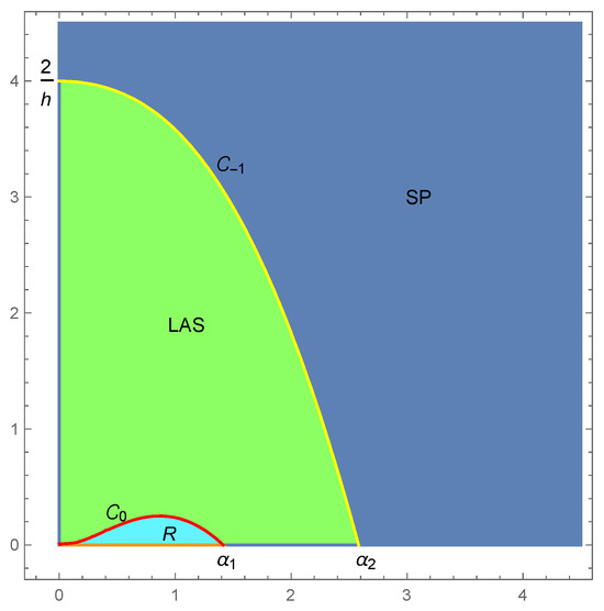
Figure 1. Parametric spaces of local dynamics in the $(\alpha ,\beta )$-plane for $h=0.5<2(\sqrt{2}-1)$, $C_0=\left\{\left(\alpha ,\beta \right):\phi \left(0\right)=1\right\}$, $C_{-1}=\left\{\left(\alpha ,\beta \right):\phi \left(-1\right)=0\right\}$.

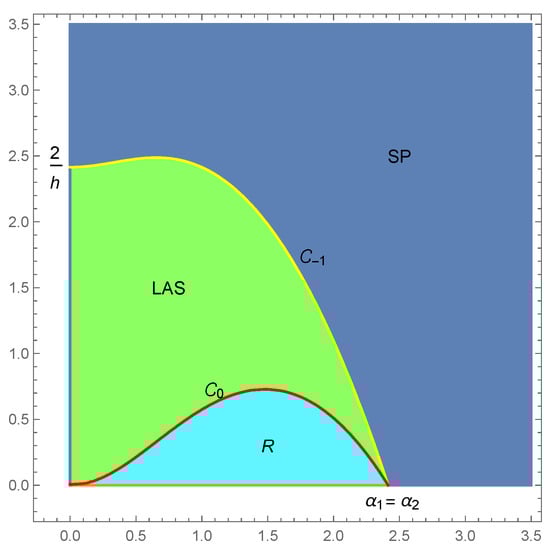
Figure 2. Parametric spaces of local dynamics in the $(\alpha ,\beta )$-plane for $h=2(\sqrt{2}-1)$, $C_0=\left\{\left(\alpha ,\beta \right):\phi \left(0\right)=1\right\}$, $C_{-1}=\left\{\left(\alpha ,\beta \right):\phi \left(-1\right)=0\right\}$.

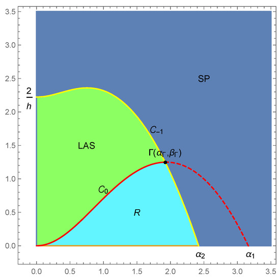
Figure 3. Parametric spaces of local dynamics in the $(\alpha ,\beta )$-plane for $h=0.9>2(\sqrt{2}-1)$, $C_0=\left\{\left(\alpha ,\beta \right):\phi \left(0\right)=1\right\}$, $C_{-1}=\left\{\left(\alpha ,\beta \right):\phi \left(-1\right)=0\right\}$.

Denoting

$$\begin{array}{cc}\hfill {\mathcal{L}}_1& =\left\{\left(\alpha ,\beta \right):0<\alpha <{\alpha }_1,{\beta }_0\left(\alpha \right)<\beta <{\beta }_{-1}\left(\alpha \right)\right\},\hfill \\ \hfill {\mathcal{L}}_2& =\left\{\left(\alpha ,\beta \right):{\alpha }_1\le \alpha \le {\alpha }_2,0<\beta <{\beta }_{-1}\left(\alpha \right)\right\},\hfill \\ \hfill {\mathcal{L}}_3& =\left\{\left(\alpha ,\beta \right):0<\alpha <{\alpha }_{\mathsf{\Gamma }},{\beta }_0\left(\alpha \right)<\beta <{\beta }_{-1}\left(\alpha \right)\right\},\hfill \\ \hfill {\mathcal{R}}_1& =\left\{\left(\alpha ,\beta \right):0<\alpha <{\alpha }_1,0<\beta <{\beta }_0\left(\alpha \right)\right\},\hfill \\ \hfill {\mathcal{R}}_2& =\left\{\left(\alpha ,\beta \right):0<\alpha \le {\alpha }_{\mathsf{\Gamma }},0<\beta <{\beta }_0\left(\alpha \right)\right\},\hfill \\ \hfill {\mathcal{R}}_3& =\left\{\left(\alpha ,\beta \right):{\alpha }_{\mathsf{\Gamma }}<\alpha <{\alpha }_2,0<\beta <{\beta }_{-1}\left(\alpha \right)\right\},\hfill \\ \hfill {\mathcal{S}}_1& =\left\{\left(\alpha ,\beta \right):0<\alpha \le {\alpha }_2,\beta >{\beta }_{-1}\left(\alpha \right)\right\},\hfill \\ \hfill {\mathcal{S}}_2& =\left\{\left(\alpha ,\beta \right):\alpha >{\alpha }_2,\beta >0\right\},\hfill \end{array}$$

we have thus completed the proofs of the following two lemmas.

Lemma 1. 

If $h\in \left(0,2\left(\sqrt{2}-1\right)\right)$, ${\alpha }_1=\sqrt{\frac{1}{1-h}}$, and ${\alpha }_2=\sqrt{\frac{2\left(h+2\right)}{(2-h)h}}$, then the unique equilibrium point $\overline{\mathbf{z}}=\left(\frac{\alpha }{\beta +{\alpha }^2},\alpha \right)$ of System (1) is as follows:

1.

Locally asymptotically stable if

$$0<h<2\left(\sqrt{2}-1\right)\mathit{and}\left(\alpha ,\beta \right)\in {\mathcal{L}}_1\cup {\mathcal{L}}_2$$

or 

$$h=2\left(\sqrt{2}-1\right)\mathit{and}\left(\alpha ,\beta \right)\in {\mathcal{L}}_1;$$

2.

A repeller if $\left(\alpha ,\beta \right)\in {\mathcal{R}}_1$;

3.

A saddle point if $\left(\alpha ,\beta \right)\in {\mathcal{S}}_1\cup {\mathcal{S}}_2$;

4.

A non-hyperbolic with

(a) 

${\lambda }_1$ and ${\lambda }_2$ being conjugated complex, and $|{\lambda }_1| = |{\lambda }_2| = 1$ if $\alpha \in \left(0,{\alpha }_1\right)$ and $\beta ={\beta }_0\left(\alpha \right)$;

(b) 

${\lambda }_1=-1$ and $|{\lambda }_2| \ne 1$ if $\alpha \in \left(0,{\alpha }_2\right)$ and $\beta ={\beta }_{-1}\left(\alpha \right)$.

Lemma 2. 

If $h\in \left(2\left(\sqrt{2}-1\right),1\right)$, ${\alpha }_1=\sqrt{\frac{1}{1-h}}$, ${\alpha }_2=\sqrt{\frac{2\left(h+2\right)}{(2-h)h}}$, ${\alpha }_{\mathsf{\Gamma }}=\frac{\sqrt{2}\left(2-h\right)}{h^2}$, and ${\beta }_{\mathsf{\Gamma }}=\frac{2\left(h^2+4h-4\right)}{h^4}$, then the equilibrium point $\overline{\mathbf{z}}=\left(\frac{\alpha }{\beta +{\alpha }^2},\alpha \right)$ of System (1) is as follows:

1.

Locally asymptotically stable if $\left(\alpha ,\beta \right)\in {\mathcal{L}}_3$;

2.

A repeller if $\left(\alpha ,\beta \right)\in {\mathcal{R}}_2\cup {\mathcal{R}}_3$;

3.

A saddle point if $\left(\alpha ,\beta \right)\in {\mathcal{S}}_1\cup {\mathcal{S}}_2$;

4.

A non-hyperbolic with

(a) 

${\lambda }_1$ and ${\lambda }_2$ being conjugated complex, and $|{\lambda }_1| = |{\lambda }_2| = 1$ if $\alpha \in \left(0,{\alpha }_{\mathsf{\Gamma }}\right)$ and $\beta ={\beta }_0\left(\alpha \right)$;

(b) 

${\lambda }_1=-1$ and $|{\lambda }_2| \ne 1$ if $\alpha \in \left(0,{\alpha }_2\right)$, $\alpha \ne {\alpha }_{\mathsf{\Gamma }}$, and $\beta ={\beta }_{-1}\left(\alpha \right)$;

(c) 

The characteristic polynomial of the form $\phi \left(\lambda \right)={\left(\lambda +1\right)}^2$ at the point $\mathsf{\Gamma }\left({\alpha }_{\mathsf{\Gamma }},{\beta }_{\mathsf{\Gamma }}\right)=\left(\frac{\sqrt{2}\left(2-h\right)}{h^2},\frac{2\left(h^2+4h-4\right)}{h^4}\right)$, so the eigenvalues are ${\lambda }_{1,2}=-1$.

See Figure 3.

3. Li–Yorke Chaos for $\mathit{h}=\frac{\mathbf{7}}{\mathbf{10}}<\mathbf{2}\left(\sqrt{\mathbf{2}}-\mathbf{1}\right)$

In order to prove the existence of Li–Yorke chaos, we will consider the corresponding eigenvalues with a modulus greater than one for $h<2\left(\sqrt{2}-1\right)$ and the set

$${\mathcal{R}}_1=\left\{\left(\alpha ,\beta \right):0<\alpha <{\alpha }_1,0<\beta <{\beta }_0\left(\alpha \right)\right\}=\left\{\left(\alpha ,\beta \right):\alpha \in \left(0,\frac{1}{\sqrt{1-h}}\right),\beta \in \left(0,{\beta }_h\right)\right\},$$

and

$${\beta }_h=\frac{-2{\alpha }^2\left(1-h\right)-1+\sqrt{8{\alpha }^2\left(1-h\right)+1}}{2\left(1-h\right)}.$$

(6)

We prove that the positive equilibrium point $\overline{\mathbf{z}}=\left(\frac{\alpha }{\beta +{\alpha }^2},\alpha \right)$ of System (1) is a snap-back repeller. The next step is to determine a neighborhood $U_{\overline{\mathbf{z}}}$ of $\overline{\mathbf{z}}=\left(\overline{x},\overline{y}\right)$ in which the norms of eigenvalues exceed one for all $\left(x,y\right)\in U_{\overline{\mathbf{z}}}$. It means that we need to solve the following system of inequalities, $\phi \left(1,x,y,\beta ,h\right)>0,$$\phi \left(-1,x,y,\beta ,h\right)>0$, and $\phi \left(0,x,y,\beta ,h\right)>1$, where

$$\phi \left(\lambda ,x,y,\beta ,h\right)={\lambda }^2+\left(h{y}^2-2hxy+h\beta +h-2\right)\lambda -h\left(1-h\right)y^2+2hxy+\left(1-h\right)\left(1-h\beta \right)$$

is the characteristic polynomial of (3), i.e., we will solve the following system of inequalities:

$$\left.\begin{array}{c}\phi \left(1,x,y,\beta ,h\right)=h^2\left(y^2+\beta \right)>0,\hfill \\ \phi \left(-1,x,y,\beta ,h\right)=-y^{2}h\left(2-h\right)+4hxy+\left(2-h\right)\left(2-h\beta \right)>0,\hfill \\ \phi \left(0,x,y,\beta ,h\right)-1=h\left[-\left(1-h\right)y^2+2xy+\left(h\beta -\beta -1\right)\right]>0.\hfill \end{array}\right\}$$

(7)

The first inequality in (7) is always satisfied. Curves ${\mathcal{C}}_1$ and ${\mathcal{C}}_2$, where

$${\mathcal{C}}_1=\left\{\left(x,y\right):\phi \left(-1,x,y,\beta ,h\right)=0\right\}\mathrm{and}{\mathcal{C}}_2=\left\{\left(x,y\right):\phi \left(0,x,y,\beta ,h\right)-1=0\right\}$$

are hyperbolas that intersect in the first quadrant at the point

$$P=\left(\frac{{\left(h-2\right)}^2}{2h\sqrt{4-h^2\beta }},\frac{\sqrt{4-h^2\beta }}{h}\right)$$

for $\beta <\frac{4}{h^2}$. The assumptions $0<h<2\left(\sqrt{2}-1\right)$ and $0<\alpha <\frac{1}{\sqrt{1-h}}$ imply that ${\beta }_h<\frac{4}{h^2}.$ Namely,

$$\frac{-2{\alpha }^2\left(1-h\right)-1+\sqrt{8{\alpha }^2\left(1-h\right)+1}}{2\left(1-h\right)}<\frac{4}{h^2}$$

is equivalent to

$$\frac{4\left(h-1\right)\left[h^4\left(h-1\right){\alpha }^4+h^2\left(h^2+8h-8\right){\alpha }^2-4{\left(h-2\right)}^2\right]}{h^4}>0$$

which is satisfied if

$$h^4\left(h-1\right){\alpha }^4+h^2\left(h^2+8h-8\right){\alpha }^2-4{\left(h-2\right)}^2<0.$$

(8)

Since $0<h<2\left(\sqrt{2}-1\right)$, it follows that $h^2+8h-8<0$, so inequality (8) is true.

Notice that

$$\phi \left(0,x,y,\beta ,h\right)-1=0⟹x=\frac{y^2\left(1-h\right)+\left(1-h\right)\beta +1}{2y},$$

and

$$\phi \left(-1,x,y,\beta ,h\right)=0⟹x=\frac{\left(2-h\right)\left(h{y}^2+h\beta -2\right)}{4hy},$$

so a neighborhood $U_{\overline{\mathbf{z}}}$ of $\overline{\mathbf{z}}=\left(\overline{x},\overline{y}\right)$, in which the norms of eigenvalues exceed one for all $\left(x,y\right)\in U_{\overline{\mathbf{z}}}$, is determined with $U_{\overline{\mathbf{z}}}={\left(U_{\overline{\mathbf{z}}}\right)}_1\cup {\left(U_{\overline{\mathbf{z}}}\right)}_2$, where

$${\left(U_{\overline{\mathbf{z}}}\right)}_1=\left\{\left(x,y\right):x\in \left(\frac{y^2\left(1-h\right)+\left(1-h\right)\beta +1}{2y},+\infty \right),y\in \left(0,\frac{\sqrt{4-h^2\beta }}{h}\right)\right\},$$

(9)

and

$${\left(U_{\overline{\mathbf{z}}}\right)}_2=\left\{\left(x,y\right):x\in \left(\frac{\left(2-h\right)\left(h{y}^2+h\beta -2\right)}{4hy},+\infty \right),y\in \left[\frac{\sqrt{4-h^2\beta }}{h},+\infty \right)\right\}$$

(10)

for $h<2\left(\sqrt{2}-1\right)$.

In this way, we obtained the following result.

Lemma 3. 

Let $0<h<2\left(\sqrt{2}-1\right),$$0<\alpha <\frac{1}{\sqrt{1-h}}$, and $0<\beta <{\beta }_h$, where ${\beta }_h$ is given by (6). Then, $U_{\overline{\mathbf{z}}}={\left(U_{\overline{\mathbf{z}}}\right)}_1\cup {\left(U_{\overline{\mathbf{z}}}\right)}_2$, where ${\left(U_{\overline{\mathbf{z}}}\right)}_{1,2}$ is defined by (9) and (10) is a repelling area of the equilibrium point $\overline{\mathbf{z}}$.

To continue investigating the conditions under which the equilibrium point $\overline{\mathbf{z}}$ will be a snap-back repeller, we will take a fixed value of the parameter h, for example, $h=\frac{7}{10}$.

Now, if $h=\frac{7}{10}$, then $\alpha <\frac{1}{\sqrt{1-\frac{7}{10}}}=\sqrt{\frac{10}{3}}\approx 1.8257$ and $\beta <{\beta }_{\frac{7}{10}}=\frac{1}{3}\sqrt{5(12{\alpha }^2+5)}-{\alpha }^2-\frac{5}{3}$. A repelling area of the equilibrium point $\overline{\mathbf{z}}$ is $U_{\overline{\mathbf{z}}}={\left(U_{\overline{\mathbf{z}}}\right)}_1\cup {\left(U_{\overline{\mathbf{z}}}\right)}_2$, where

$$\begin{array}{cc}\hfill {\left(U_{\overline{\mathbf{z}}}\right)}_1& =\left\{\left(x,y\right):x\in \left(\frac{3y^2+3\beta +10}{20y},+\infty \right),y\in \left(0,\frac{\sqrt{400-49\beta }}{7}\right)\right\},\hfill \\ \hfill {\left(U_{\overline{\mathbf{z}}}\right)}_2& =\left\{\left(x,y\right):x\in \left(\frac{91y^2+91\beta -260}{280y},+\infty \right),y\in \left[\frac{\sqrt{400-49\beta }}{7},+\infty \right)\right\}.\hfill \end{array}$$

To prove that the equilibrium point $\overline{\mathbf{z}}=\left(\overline{x},\overline{y}\right)$ is a snap-back repeller for $M=2$, we need to find points ${\mathbf{z}}_0=\left(x_0,y_0\right)\in U_{\overline{\mathbf{z}}}$ and ${\mathbf{z}}_1=\left(x_1,y_1\right)\notin U_{\overline{\mathbf{z}}}$ such that

$${\mathbf{z}}_1=T\left({\mathbf{z}}_0\right),{\mathbf{z}}_2=T\left({\mathbf{z}}_1\right)=T^2\left({\mathbf{z}}_0\right)=\overline{\mathbf{z}}\mathrm{and}det{J}_T\left({\mathbf{z}}_1\right)\ne 0.$$

By calculating the inverse iterations of the fixed point $\overline{\mathbf{z}}$ twice, we are looking for the point ${\mathbf{z}}_0=\left(x_0,y_0\right)$, $x_0>0$, $y_0>0$, as the solution of the following system:

$$\begin{array}{c}\hfill \left.\begin{array}{c}x+\frac{7}{10}\left(\alpha -\beta x-x{y}^2\right)=x_1\\ y+\frac{7}{10}\left(\beta x+x{y}^2-y\right)=y_1\end{array}\right\}\end{array}$$

(11)

for ${\mathbf{z}}_1=\left(x_1,y_1\right)$ which is the solution of the system

$$\left.\begin{array}{c}x+\frac{7}{10}\left(\alpha -\beta x-x{y}^2\right)=\frac{\alpha }{{\alpha }^2+\beta }\\ y+\frac{7}{10}\left(\beta x+x{y}^2-y\right)=\alpha \end{array}\right\}.$$

(12)

The solutions of System (12) are

$${\left({\mathbf{z}}_1\right)}_{\pm }=\left({\left(x_1\right)}_{\pm },{\left(y_1\right)}_{\pm }\right),$$

where

$${\left(x_1\right)}_{\pm }=\frac{-5\alpha \pm \frac{1}{7}Q}{10\left({\alpha }^2+\beta \right)}+\frac{10\alpha +3\alpha \left({\alpha }^2+\beta \right)}{10\left({\alpha }^2+\beta \right)},{\left(y_1\right)}_{\pm }=\frac{5\alpha \mp \frac{1}{7}Q}{3\left({\alpha }^2+\beta \right)},$$

and

$$Q=\sqrt{7Q_1}>0,Q_1=-3{\alpha }^4\left(21\beta -100\right)+{\alpha }^2\left(390\beta -126{\beta }^2+175\right)-9{\beta }^2\left(7\beta -10\right).$$

By using $\beta <{\beta }_{\frac{7}{10}}$, it is easy to see that $Q_1>0$.

Now, we prove that $detJ\left({\left({\mathbf{z}}_1\right)}_{\pm }\right)\ne 0$ considering that

$$detJ\left({\left({\mathbf{z}}_1\right)}_{+}\right)=\frac{Q\left(-Q-7\alpha \left(3\left({\alpha }^2+\beta \right)-5\right)\right)}{1050{\left({\alpha }^2+\beta \right)}^2},$$

$$detJ\left({\left({\mathbf{z}}_1\right)}_{-}\right)=\frac{Q\left(-Q+7\alpha \left(3\left({\alpha }^2+\beta \right)-5\right)\right)}{1050{\left({\alpha }^2+\beta \right)}^2}.$$

Suppose that $detJ\left({\left({\mathbf{z}}_1\right)}_{\pm }\right)=0$. Then,

$$detJ\left({\left({\mathbf{z}}_1\right)}_{\pm }\right)=0⟺Q=\mp 7\alpha \left(3\left({\alpha }^2+\beta \right)-5\right).$$

If $\alpha \left(3\left({\alpha }^2+\beta \right)-5\right)=0$, we have a contradiction with $Q>0$, such that $detJ\left({\left({\mathbf{z}}_1\right)}_{\pm }\right)\ne 0$. However, if $\alpha \left(3\left({\alpha }^2+\beta \right)-5\right)>0$, since $Q>0$, we have that

$$Q=7\alpha \left(3\left({\alpha }^2+\beta \right)-5\right)⟺21{\beta }^2+\beta \left(42{\alpha }^2-30\right)+{\alpha }^2\left(21{\alpha }^2-170\right)=0,$$

which for ${\alpha }^2<\frac{10}{3}$ has only one positive solution

$${\beta }_{+}=\frac{-\left(21{\alpha }^2-15\right)+\sqrt{15\left(196{\alpha }^2+15\right)}}{21}.$$

This implies that ${\beta }_{+}\notin \left(0,{\beta }_{\frac{7}{10}}\right)$, which is a contradiction. Therefore, it is true that $detJ\left({\left({\mathbf{z}}_1\right)}_{\pm }\right)\ne 0$ if $\alpha \left(3\left({\alpha }^2+\beta \right)-5\right)>0$.

Similarly, we conclude that $detJ\left({\left({\mathbf{z}}_1\right)}_{\pm }\right)\ne 0$ if $\alpha \left(3\left({\alpha }^2+\beta \right)-5\right)<0$.

Now, note the following fact: for $\beta <{\beta }_{\frac{7}{10}}$, we have

$$Q\ne \mp 7\alpha \left(3\left({\alpha }^2+\beta \right)-5\right).$$

(13)

In the next step, we will solve System (11) for ${\mathbf{z}}_1=\left(x_1,y_1\right)=\left({\left(x_1\right)}_{-},{\left(y_1\right)}_{-}\right)$. From the second equation in System (11), we obtain

$$x=\frac{-3y+10{\left(y_1\right)}_{-}}{7\left(\beta +y^2\right)}=\frac{10Q+350\alpha -63y\left(\beta +{\alpha }^2\right)}{147\left(y^2+\beta \right)\left({\alpha }^2+\beta \right)}.$$

This implies $-3y+10{\left(y_1\right)}_{-}>0⟺$ $y<\frac{10}{3}{\left(y_1\right)}_{-}$, i.e., $y<\frac{50\alpha +\frac{10}{7}Q}{9\left({\alpha }^2+\beta \right)}$. After substituting x in the first equation of System (11), we obtain

$$\frac{-3y+10{\left(y_1\right)}_{-}}{7\left(\beta +y^2\right)}+\frac{7}{10}\left(\alpha -\beta \left(\frac{-3y+10{\left(y_1\right)}_{-}}{7\left(\beta +y^2\right)}\right)-\left(\frac{-3y+10{\left(y_1\right)}_{-}}{7\left(\beta +y^2\right)}\right)y^2\right)-{\left(x_1\right)}_{-}=0.$$

Let

$$H\left(\beta ,y\right)=\frac{-3y+10{\left(y_1\right)}_{-}}{7\left(\beta +y^2\right)}+\frac{7}{10}\left(\alpha -\left(\frac{-3y+10{\left(y_1\right)}_{-}}{7\left(\beta +y^2\right)}\right)(\beta +y^2\right)-{\left(x_1\right)}_{-},$$

i.e.,

$$H\left(\beta ,y\right)=\frac{21y^3-7\left(10{\left(x_1\right)}_{-}+10{\left(y_1\right)}_{-}-7\alpha \right)y^2+3\left(7\beta -10\right)y+100{\left(y_1\right)}_{-}-7\beta \left(10{\left(x_1\right)}_{-}+10{\left(y_1\right)}_{-}-7\alpha \right)}{70\left(y^2+\beta \right)}.$$

(14)

By using the facts

$${\left(x_1\right)}_{-}=\frac{-5\alpha -\frac{1}{7}Q}{10\left({\alpha }^2+\beta \right)}+\frac{10\alpha +3\alpha \left({\alpha }^2+\beta \right)}{10\left({\alpha }^2+\beta \right)},{\left(y_1\right)}_{-}=\frac{5\alpha +\frac{1}{7}Q}{3\left({\alpha }^2+\beta \right)},$$

and $\overline{y}=\alpha$, we obtain

$$H\left(\beta ,\overline{y}\right)=0⟺\frac{\left(100-49\left({\alpha }^2+\beta \right)\right)\left(Q-7\alpha \left(3{\alpha }^2+3\beta -5\right)\right)}{1470{\left({\alpha }^2+\beta \right)}^2}=0.$$

(15)

Considering (13), Equation (15) is satisfied if $49\left({\alpha }^2+\beta \right)=100,$ or, equivalently,

$$\beta =\frac{100-49{\alpha }^2}{49}.$$

It implies that $100-49{\alpha }^2>0$, i.e., $\alpha <\frac{10}{7}\approx 1.4286$. On the other hand,

$$\beta <{\beta }_{\frac{7}{10}}⟺\frac{100-49{\alpha }^2}{49}<\frac{1}{3}\sqrt{5(12{\alpha }^2+5)}-{\alpha }^2-\frac{5}{3}$$

which implies $\alpha >\sqrt{\frac{3950}{2401}}\approx 1.2826$. If $\alpha \in \left(\sqrt{\frac{3950}{2401}},\frac{10}{7}\right)$, we denote

$${\beta }_{*}=\frac{100-49{\alpha }^2}{49}.$$

Now, from (14) we obtain

$$\frac{\partial H\left(\beta ,y\right)}{\partial y}=\frac{21{\left(\beta +y^2\right)}^2+30\left(y^2-\beta \right)-200y{\left(y_1\right)}_{-}}{70{\left(y^2+\beta \right)}^2}.$$

By using the fact that ${\left(y_1\right)}_{-}=\frac{5\alpha +\frac{1}{7}Q}{3\left({\alpha }^2+\beta \right)}$ and $\overline{y}=\alpha$, we have that

$$\frac{\partial H\left(\beta ,\alpha \right)}{\partial y}=\frac{7\left(63{\beta }^3+9\left(21{\alpha }^2-10\right){\beta }^2+{\alpha }^2\left(63{\alpha }^4+90{\alpha }^2+189{\alpha }^2\beta -1000\right)\right)-200\alpha Q}{1470{\left({\alpha }^2+\beta \right)}^3}.$$

Let us show that $\frac{\partial H\left({\beta }_{*},\overline{y}\right)}{\partial y}\ne 0$. Otherwise, if $\frac{\partial H\left({\beta }_{*},\overline{y}\right)}{\partial y}=0$, then

$$2700-10633{\alpha }^2=96040{\alpha }^2{Q}^2.$$

Since $\alpha \in \left(\sqrt{\frac{3950}{2401}},\frac{10}{7}\right)$, the left side of the past equality is negative, which is impossible. It means that $\frac{\partial H\left({\beta }_{*},\overline{y}\right)}{\partial y}\ne 0$ holds.

Therefore, under certain conditions on the parameters, we have that

$1^{\circ }$

${\beta }_{*}=\frac{100-49{\alpha }^2}{49}\in \left(0,\frac{950}{2401}\right)$ for $\alpha \in \left(\sqrt{\frac{3950}{2401}},\frac{10}{7}\right);$

$2^{\circ }$

$H\left({\beta }_{*},\overline{y}\right)=0;$

$3^{\circ }$

$H\left(\beta ,y\right)$ is continuous for $\beta <{\beta }_{*}$ and $y<\frac{50\alpha +\frac{10}{7}Q}{9\left({\alpha }^2+\beta \right)}$;

$4^{\circ }$

$\frac{\partial H\left({\beta }_{*},\overline{y}\right)}{\partial y}\ne 0$.

By the Implicit Function Theorem, there exists a unique function $y=y_0\left(\beta \right)$ and $\delta >0$ such that

(i)

$y_0\left({\beta }_{*}\right)=\overline{y}$.

(ii)

$H\left(\beta ,y_0\left(\beta \right)\right)=0$ for $\beta \in \left({\beta }_{*}-\delta ,{\beta }_{*}+\delta \right)$.

(iii)

$y=y_0\left(\beta \right)$ is continuous in $\beta \in \left({\beta }_{*}-\delta ,{\beta }_{*}+\delta \right)$.

Figure 4 shows the area of the parameters for which the equilibrium point is a repeller and the set $\mathcal{B}=\left\{\left(\alpha ,\beta \right):\alpha \in \left(\sqrt{\frac{3950}{2401}},\frac{10}{7}\right),\beta ={\beta }_{*}\right\}\subset {\mathcal{R}}_1$ in the $(\alpha ,\beta )$-plane.

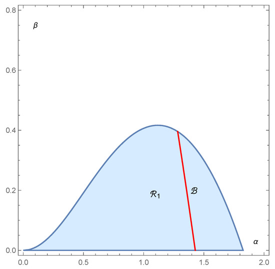
Figure 4. The area of the parameters for which the equilibrium point is a repeller and the set $\mathcal{B}$ (red) is shown (in the $(\alpha ,\beta )$-plane for $h=0.7$).

Let $M=2$ and ${\mathbf{z}}_0=\left(x_0,y_0\right)=\left(\frac{10Q+350\alpha -63y_0\left({\alpha }^2+\beta \right)}{147\left(\beta +y_0^2\right)\left({\alpha }^2+\beta \right)},y_0\right)$ for $y_0<\frac{50\alpha +\frac{10}{7}Q}{9\left({\alpha }^2+\beta \right)}$. Then, ${\mathbf{z}}_0$ belongs to $U_{\overline{\mathbf{z}}}$ for a small enough $\beta -{\beta }_{*}$. Assume that $ϵ>0$ is arbitrary and let

$$x^{*}=max\left\{\overline{x}+ϵ,x_0+ϵ\right\}.$$

Finally, let

$$U_{\overline{\mathbf{z}}}^{*}={\left(U_1\right)}^{*}\cup {\left(U_2\right)}^{*},$$

where

$${\left(U_1\right)}^{*}=\left\{\left(x,y\right):x\in \left(\frac{3y^2+3\beta +10}{20y},x^{*}\right),y\in \left(y_1^{*},\frac{\sqrt{400-49\beta }}{7}\right)\right\},$$

and

$${\left(U_2\right)}^{*}=\left\{\left(x,y\right):x\in \left(\frac{91y^2+91\beta -260}{280y},x^{*}\right),y\in \left[\frac{\sqrt{400-49\beta }}{7},y_2^{*}\right)\right\}.$$

Also, $y_1^{*}$ and $y_2^{*}$ are the second coordinates of the intersection points of the line given by the equation $x=x^{*}$ with the curves ${\mathcal{C}}_2$ and ${\mathcal{C}}_1$, respectively.

Theorem 2. 

Assume that $h=\frac{7}{10}$, $\alpha \in \left(\sqrt{\frac{3950}{2401}},\frac{10}{7}\right)$ and ${\beta }_{*}=\frac{100-49{\alpha }^2}{49}$. Then, there exists β near ${\beta }_{*}$ such that $\overline{z}=(\overline{x},\overline{y})=\left(\frac{\alpha }{{\alpha }^2+\beta },\alpha \right)$ is a snap-back repeller of System (1) and, consequently, System (1) is chaotic in the sense of Li–Yorke.

4. Numerical Simulations

In many articles, the appearance of chaos is established by the existence of positive Lyapunov coefficients (e.g., [15]). Although we proved the existence of chaos in the previous section using the Marotto method, we will make several corresponding numerical simulations by calculating the Lyapunov coefficients. Most of the experimentalists in dynamical systems theory take the existence of positive Lyapunov coefficients as enough evidence for the existence of chaos (see [23,24,25,26]). In that case, different software packages, such as Dynamica in [19] or Chaos in [25,26], are used to justify the use of the word chaos. Also, see the references in [23].

If $\alpha =\frac{7}{5}=1.4$, then

$${\beta }_{*}=\frac{100-49{\left(\frac{7}{5}\right)}^2}{49}=\frac{99}{1225}\approx 0.080816.$$

Let us choose $\beta =\frac{8}{100}$ close to ${\beta }_{*}=\frac{99}{1225}$. Now, $U_{\overline{\mathbf{z}}}={\left(U_{\overline{\mathbf{z}}}\right)}_1\cup {\left(U_{\overline{\mathbf{z}}}\right)}_2$, where

$${\left(U_{\overline{\mathbf{z}}}\right)}_1=\left\{\left(x,y\right):x\in \left(\frac{75y^2+256}{500y},+\infty \right),y\in \left(0,\frac{\sqrt{9902}}{35}\right)\right\},$$

and

$${\left(U_{\overline{\mathbf{z}}}\right)}_2=\left\{\left(x,y\right):x\in \left(\frac{2275y^2-6318}{7000y},+\infty \right),y\in \left[\frac{\sqrt{9902}}{35},+\infty \right)\right\}.$$

See Figure 5a.

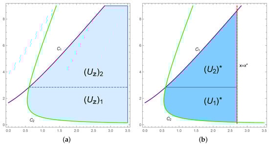
Figure 5. Repelling area $U_{\overline{\mathbf{z}}}$ (a) and neighborhood $U_{\overline{\mathbf{z}}}^{*}$ (b) of the snap-back repeller $\overline{\mathbf{z}}$ (for $\alpha =1.4$, $\beta =0.08$, and $h=0.7$).

The solutions of System (12) are the equilibrium point and

$${\left({\mathbf{z}}_1\right)}_{\pm }=\left({\left(x_1\right)}_{\pm },{\left(y_1\right)}_{\pm }\right),$$

where

$$\left({\left(x_1\right)}_{\pm },{\left(y_1\right)}_{\pm }\right)=\left(\frac{973}{1275}\pm \frac{\sqrt{7}\sqrt{24003649}}{17850},\frac{175}{153}\mp \frac{\sqrt{7}\sqrt{24003649}}{5355}\right).$$

The solution of System (11) for $\left(x_1,y_1\right)=\left({\left(x_1\right)}_{-},{\left(y_1\right)}_{-}\right)$ which belongs to $U_{\overline{\mathbf{z}}}$ is

$$\left(x_0,y_0\right)=\left(2.2013061560494975\prime ,1.400206800960196\prime \right).$$

Therefore,

$$\left.\begin{array}{c}{\mathbf{z}}_0=\left(x_0,y_0\right)=\left(2.2013061560494975\prime ,1.400206800960196\prime \right)\hfill \\ {\mathbf{z}}_1=\left(x_1,y_1\right)=T\left(x_0,y_0\right)=\left(\frac{973}{1275}-\frac{\sqrt{7}\sqrt{24003649}}{17850},\frac{175}{153}+\frac{\sqrt{7}\sqrt{24003649}}{5355}\right)\hfill \\ \overline{\mathbf{z}}=\left(\overline{x},\overline{y}\right)=T\left(x_1,y_1\right)=T^2\left(x_0,y_0\right)=\left(\frac{35}{51},\frac{7}{5}\right).\hfill \end{array}\right\}$$

(16)

The Jacobian matrix of T at the point $\overline{\mathbf{z}}=\left(\overline{x},\overline{y}\right)$ has an eigenvalue ${\lambda }_{\pm }=0.60855\mp 0.91998i$ with $\left|{\lambda }_{\pm }\right|=1.103$, at point $\left(x_0,y_0\right)$ has eigenvalues ${\lambda }_1=2.5357$ and ${\lambda }_2=1.6511$, and at point $\left(x_1,y_1\right)$ has eigenvalues ${\lambda }_1=-7.7491$ and ${\lambda }_2=0.28397$.

For $ϵ=0.5$, we have that

$$x^{*}=max\left\{\overline{x}+ϵ,x_0+ϵ\right\}\approx 2.7013.$$

Next, $y_1^{*}\approx 0.19158$ and $y_2^{*}\approx 8.6334$ are the second coordinates of the intersection points of the line given by the equation $x=2.7013$ with the curves ${\mathcal{C}}_2$ and ${\mathcal{C}}_1$, respectively. Then,

$$U_{\overline{\mathbf{z}}}^{*}=U_1\cup U_2,$$

where

$$U_1^{*}=\left\{\left(x,y\right):x\in \left(\frac{75y^2+256}{500y},2.7013\right),y\in \left(0.19158,\frac{\sqrt{9902}}{35}\right)\right\},$$

and

$$U_2^{*}=\left\{\left(x,y\right):x\in \left(\frac{2275y^2-6318}{7000y},2.7013\right),y\in \left[\frac{\sqrt{9902}}{35},8.6334\right)\right\}.$$

See Figure 5b.

Figure 6 represents the phase portrait with 30 iterations with repelling area $U_{\overline{\mathbf{z}}}$ and neighborhood $U_{\overline{\mathbf{z}}}^{*}$ of the snap-back repeller $\overline{\mathbf{z}}$. Furthermore, Figure 6 shows the points in (16).

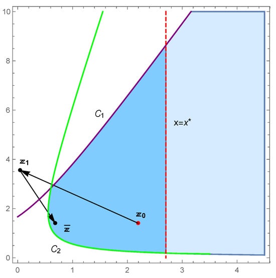
Figure 6. The snap-back repeller for $\alpha =1.4$, $\beta =0.08$, and $h=0.7$.

Now, assume that $\alpha =0.6\notin \left(\sqrt{\frac{3950}{2401}},\frac{10}{7}\right)$ and $\beta =0.001<{\beta }_{\frac{7}{10}}=0.24881$. Then, there exists $M>2$ such that $T^M\left({\overline{\mathbf{z}}}_0\right)=\overline{\mathbf{z}}$. In that case, if $M=17$, the region $U_{\overline{\overline{\mathbf{z}}}}^{*}$ is a circle.

Figure 7 represents a phase portrait with 30 iterations and the snap-back repeller $\overline{\mathbf{z}}$. Here,

$${\mathbf{z}}_1=T\left({\mathbf{z}}_0\right),{\mathbf{z}}_2=T^2\left({\mathbf{z}}_0\right),\dots ,{\mathbf{z}}_{18}=T^{17}\left({\mathbf{z}}_0\right)=\overline{\mathbf{z}},$$

where

$$\begin{array}{ccc}{\mathbf{z}}_0=\left(1.7658,0.52217\right),\hfill & {\mathbf{z}}_1=\left(1.84754,0.494912\right),\hfill & {\mathbf{z}}_2=\left(1.94947,0.46654\right),\hfill \\ {\mathbf{z}}_3=\left(2.07108,0.438351\right),\hfill & {\mathbf{z}}_4=\left(2.21106,0.411529\right),\hfill & {\mathbf{z}}_5=\left(2.36739,0.387125\right),\hfill \\ {\mathbf{z}}_6=\left(2.53738,0.366149\right),\hfill & {\mathbf{z}}_7=\left(2.71748,0.349742\right),\hfill & {\mathbf{z}}_8=\left(2.9029,0.339506\right),\hfill \\ {\mathbf{z}}_9=\left(3.08665,0.338104\right),\hfill & {\mathbf{z}}_{10}=\left(3.25749,0.350585\right),\hfill & {\mathbf{z}}_{11}=\left(3.39495,0.387721\right),\hfill \\ {\mathbf{z}}_{12}=\left(3.45532,0.475941\right),\hfill & {\mathbf{z}}_{13}=\left(3.32502,0.693091\right),\hfill & {\mathbf{z}}_{14}=\left(2.62461,1.32833\right),\hfill \\ {\mathbf{z}}_{15}=\left(-0.198952,3.64206\right),\hfill & {\mathbf{z}}_{16}=\left(2.0685,-0.754833\right),\hfill & \overline{\mathbf{z}}=\left(1.66205,0.6\right).\hfill \end{array}$$

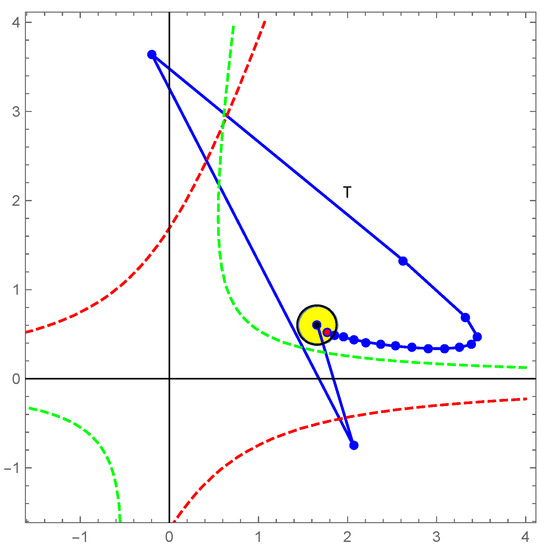
Figure 7. The snap-back repeller for $\alpha =0.6$, $\beta =0.001$, and $h=0.7$.

If we suppose that $\alpha =0.6$ and $\beta =0.12<{\beta }_{\frac{7}{10}}=0.24881$, then Figure 8a shows a snap-back repeller with

$$\begin{array}{cc}\hfill {\mathbf{z}}_0& =({1.4605157298915394}^{\prime },{1.424776880514991}^{\prime }),\hfill \\ \hfill {\mathbf{z}}_1& =(-{0.31754936043512777}^{\prime },{2.6254981544811646}^{\prime }),\hfill \\ \hfill {\mathbf{z}}_2& =\left({1.6613856774674765}^{\prime },-{0.7712855915582548}^{\prime }\right)\hfill \\ \hfill \overline{\mathbf{z}}& =\left(1.25,0.6\right).\hfill \end{array}$$

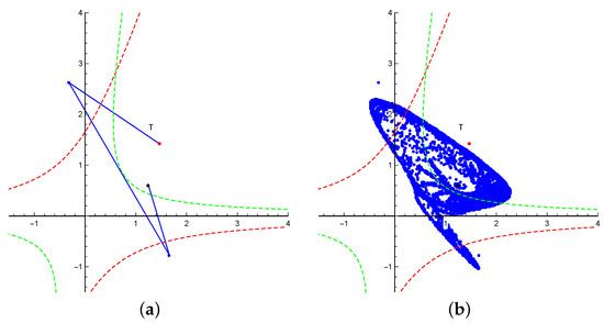
Figure 8. The snap-back repeller for $\alpha =0.6$, $\beta =0.12$, and $h=0.7$.

The graph represents a phase portrait with 70 iterations. Figure 8b represents a phase portrait with 11170 iterations (we obtained a chaotic attractor due to the accumulation of rounding errors). In Figure 9a and Figure 10a, the bifurcation diagrams are generated by code Bif2D from [23], and in Figure 9b and Figure 10b corresponding Lyapunov coefficients are generated by the code in [24].

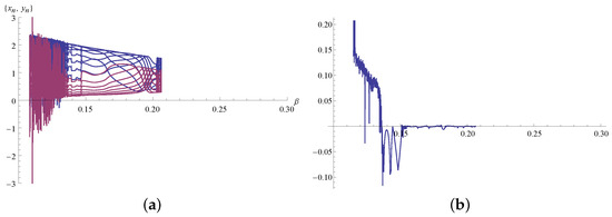
Figure 9. (a) Bifurcation diagram for $\alpha =0.60$, $\beta \in \left(0.10,0.30\right)$, $h=0.7$, $\overline{\mathbf{z}}=\left(1.25,0.6\right)$, and initial point ${\mathbf{z}}_0=(1.4605157298915394,1.424776880514991);$ (b) corresponding Lyapunov coefficients.

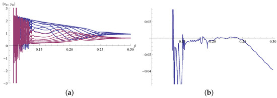
Figure 10. (a) Bifurcation diagram for $\alpha =0.60$, $\beta \in \left(0.10,0.30\right)$, $h=0.7$, $\overline{\mathbf{z}}=\left(1.25,0.6\right)$, and initial point ${\mathbf{z}}_0=(1.40,0.65);$ (b) corresponding Lyapunov coefficients.

5. Conclusions

We consider a chaotic dynamic of System (1), which is the Euler discretization of System (2), which was used as the model for glycolysis decomposition in [9]. System (1) has a unique positive equilibrium, which locally can have any character depending on the parameter region. That is, this unique equiibrium solution can be either locally symptotically stable or repeller, saddle point, or non-hyperbolic. The global dynamics of such a system can be quite complicated and could include the existence of an infinite number of period-two solutions or equilibrium solutions, as we have shown in a series of papers [13]. In this paper, we focus on the case when this equilibrium is a repeller and prove that in this case there exists a region of parameters where System (1) exhibits chaos. The quite challenging problem is whether the local stability of System (1) implies the global stability of such a system and, in general, if System (1) is structurally stable. At this time, we are leaving these problems for future research.

References

- Li, T.Y.; Yorke, J.A. Period Three Implies Chaos. Am. Math. Mon. 1975, 82, 985–992. [Google Scholar] [CrossRef]
- Marotto, F.R. Snap-Back Repellers Imply Chaos in Rn. J. Math. Anal. Appl. 1978, 63, 199–223. [Google Scholar] [CrossRef]
- Marotto, F.R. Perturbations of stable and chaotic difference equations. J. Math. Anal. Appl. 1979, 72, 716–729. [Google Scholar] [CrossRef][Green Version]
- Marotto, F.R. Chaotic Behavior in the Hénon Mapping. J. Math. Anal. Appl. 1979, 68, 187–194. [Google Scholar] [CrossRef]
- Aulbach, B.; Kieninger, B. On three definitions of chaos. Nonlinear Dyn. Syst. Theory 2001, 1, 23–37. [Google Scholar]
- Li, C.P.; Chen, G.R. An Improved Version of the Marotto Theorem. Chaos Solitons Fractals 2003, 18, 69–77. [Google Scholar] [CrossRef]
- Kloeden, P.; Li, Z. Li-Yorke chaos in higher dimensions: A review. J. Differ. Equ. Appl. 2006, 12, 247–269. [Google Scholar] [CrossRef]
- Marotto, F.R. On Redefining a Snap-Back Repeller. Chaos Solitons Fractals 2005, 25, 25–28. [Google Scholar] [CrossRef]
- Khan, A.Q.; Abdullah, E.; Ibrahim, T.F. Supercritical Neimark-Sacker Bifurcation and Hybrid Control in a Discrete-Time Glycolytic Oscillator Model. Math. Probl. Eng. 2020, 2020, 7834076. [Google Scholar] [CrossRef]
- Berkal, M.; Almatrafi, M.B. Bifurcation and Stability of Two-Dimensional Activator–Inhibitor Model with Fractional-Order Derivative. Fractal Fract. 2023, 7, 344. [Google Scholar] [CrossRef]
- Berkal, M.; Almatrafi, M.B. Bifurcation Analysis and Chaos Control for Prey-Predator Model With Allee Effect. Int. J. Anal. Appl. 2023, 21, 131. [Google Scholar]
- Nurkanović, Z.; Nurkanović, M.; Garić-Demirović, M. Stability and Neimark-Sacker Bifurcation of Certain Mixed Monotone Rational Second-Order Difference Equation. Qual. Theory Dyn. Syst. 2021, 20, 75. [Google Scholar] [CrossRef]
- Bektešević, J.; Kulenović, M.R.S.; Pilav, E. Global Dynamics of Cubic Second Order Difference Equation in the First Quadrant. Adv. Differ. Equ. 2015, 176, 1–38. [Google Scholar] [CrossRef][Green Version]
- Bektešević, J.; Hadžiabdić, V.; Mehuljić, M.; Mujić, N. Dynamics of a two-dimensional cooperative system of polynomial difference equations with cubic terms. Sarajevo J. Math. 2022, 18, 127–160. [Google Scholar]
- Garić-Demirović, M.; Hrustić, S.; Moranjkić, S.; Nurkanović, M.; Nurkanović, Z. The existence of Li-Yorke chaos in certain predator-prey system of difference equations. Sarajevo J. Math. 2022, 18, 45–62. Available online: https://www.anubih.ba/Journals/vol.18,no-1,y22/04-M_Garic_Demirovic-S_Hrustic-S_Moranjkic-M_and_Z_Nurkanovic.pdf (accessed on 19 March 2024).
- Li, J.; Zang, H.; Wei, X. On the construction of one-dimensional discrete chaos theory based on the improved version of Marotto’s theorem. J. Comput. Appl. Math. 2020, 380, 112952. [Google Scholar] [CrossRef]
- Zhang, L.; Huang, Q. Chaos induced by snap-back repellers in non-autonomous discrete dynamical systems. J. Differ. Equ. Appl. 2018, 24, 1126–1144. [Google Scholar] [CrossRef]
- Balibrea, F.; Cascales, A. Li-Yorke chaos in perturbed rational difference equations. In Difference Equations, Discrete Dynamical Systems and Applications; Springer Proceedings in Mathematics & Statistics; Springer: Berlin/Heidelberg, Germany, 2016; Volume 180, pp. 49–61. [Google Scholar] [CrossRef]
- Kulenović, M.R.S.; Merino, O. Discrete Dynamical Systems and Difference Equations with Mathematica; Chapman and Hall/CRC: Boca Raton, FL, USA; London, UK, 2002. [Google Scholar] [CrossRef]
- Elaydi, S. An Introduction to Difference Equations, 3rd ed.; Undergraduate Texts in Mathematics; Springer: New York, NY, USA, 2005; Available online: https://www.abebooks.co.uk/9780387230597/Introduction-Difference-Equations-Undergraduate-Texts-0387230599/plp (accessed on 19 March 2024).
- Elaydi, S. Discrete Chaos. With Applications in Science and Engineering, 2nd ed.; Chapman & Hall/CRC: Boca Raton, FL, USA, 2007. [Google Scholar] [CrossRef]
- Alligood, K.T.; Sauer, T.D.; Yorke, J.A. Chaos. An Introduction to Dynamical Systems; Textbooks in Mathematical Sciences; Springer: New York, NY, USA, 1997. [Google Scholar] [CrossRef]
- Ufuktepe, Ü.; Kapçak, S. Applications of Discrete Dynamical Systems with Mathematica. Thesis, Izmir University of Economics, Izmir, Türkiye, 2014. Volume 1909. pp. 207–216. Available online: http://hdl.handle.net/2433/223175 (accessed on 19 March 2024).
- Sandri, M. Numerical Calculation of Lyapunov Exponents. Math. J. 1996, 6, 78–84. Available online: https://www.mathematica-journal.com/issue/v6i3/article/sandri/contents/63sandri.pdf (accessed on 19 March 2024).
- Korsch, H.J.; Jodl, H.-J. Chaos. A Program Collection for the PC, 2nd ed.; with 1 CD-ROM (Windows 95 and NT); Springer: Berlin/Heidelberg, Germany, 1999. [Google Scholar]
- Nusse, H.E.; Yorke, J.A. Dynamics: Numerical Explorations, 2nd ed.; Accompanying computer program Dynamics 2 coauthored by Brian R. Hunt and Eric J. Kostelich; Applied Mathematical Sciences 101; Springer: New York, NY, USA, 1998. [Google Scholar]
Disclaimer/Publisher’s Note: The statements, opinions and data contained in all publications are solely those of the individual author(s) and contributor(s) and not of MDPI and/or the editor(s). MDPI and/or the editor(s) disclaim responsibility for any injury to people or property resulting from any ideas, methods, instructions or products referred to in the content. |
© 2024 by the authors. Licensee MDPI, Basel, Switzerland. This article is an open access article distributed under the terms and conditions of the Creative Commons Attribution (CC BY) license (https://creativecommons.org/licenses/by/4.0/).