An Efficient Subspace Minimization Conjugate Gradient Method for Solving Nonlinear Monotone Equations with Convex Constraints

Abstract

The subspace minimization conjugate gradient (SMCG) methods proposed by Yuan and Store are efficient iterative methods for unconstrained optimization, where the search directions are generated by minimizing the quadratic approximate models of the objective function at the current iterative point. Although the SMCG methods have illustrated excellent numerical performance, they are only used to solve unconstrained optimization problems at present. In this paper, we extend the SMCG methods and present an efficient SMCG method for solving nonlinear monotone equations with convex constraints by combining it with the projection technique, where the search direction is sufficiently descent.Under mild conditions, we establish the global convergence and R-linear convergence rate of the proposed method. The numerical experiment indicates that the proposed method is very promising.

1. Introduction

We consider the following nonlinear equations with convex constraints:

$$F\left(x\right)=0,x\in \mathsf{\Omega },$$

(1)

where $\mathsf{\Omega }\subset {\mathbb{R}}^n$ is a non-empty closed convex set and F: ${\mathbb{R}}^n\to {\mathbb{R}}^n$ is a continuous mapping that satisfies the monotonicity condition

$$⟨F\left(x\right)-F\left(y\right),x-y⟩\ge 0,$$

(2)

for all $x,y\in {\mathbb{R}}^n.$ It is easy to verify that the solution set of problem (1) is convex under condition (2).

Nonlinear equations have numerous practical applications, e.g., machinery manufacturing problems [1], neural networks [2], economic equilibrium problems [3], image recovery problems [4], and so on. In the context of many practical applications, problem (1) has attracted a substantial number of scholars to put forward more effective iterative methods to find solutions, such as Newton’s method, quasi-Newton methods, trust region methods, Levenberg–Marquardt methods, or their variants ([5,6,7,8,9]). Although these methods are very popular and have fast convergence at an adequately good initial point, they are not suitable for solving large-scale nonlinear equations due to the calculation and storage of the Jacobian matrix or its approximation.

Due to its simple form and low memory requirement, conjugate gradient (CG) methods are used to solve problem (1) by combining them with projection technology proposed by Solodov and Svaiter [10] (see [11,12]). Xiao and Zhu [13] extended the famous CG_DESCENT method [14] for solving nonlinear monotone equations with convex constraints due to its effectiveness. Liu and Li [15] presented an efficient projection method for solving convex constrained monotone nonlinear equations, which can be viewed as another extension of the CG_DESCENT method [14] and was used to solve the sparse signal reconstruction in compressive sensing. Based on the Dai–Yuan (DY) method [16], Liu and Feng [17] presented an efficient derivative-free iterative method and established its Q-linear convergence rate of the proposed method under the local error bound condition. By minimizing the distance between relative matrix and the self-scaling memoryless BFGS method in the Frobenius norm, Gao et al. [18] proposed an adaptive projection method for solving nonlinear equations and applied it to recover a sparse signal from incomplete and contaminated sampling measurements. Based on [19], Li and Zheng [20] proposed two effective derivative-free methods for solving large-scale nonsmooth monotone nonlinear equations. Waziri et al. [21] proposed two DY-type iterative methods for solving (1). By using the projection method [10], Abdulkarim et al. [22] introduced two classes of three-term methods for solving (1) and established the global convergence under a weaker monotonicity condition.

The subspace minimization conjugate gradient (SMCG) methods proposed by Yuan and Stoer [23] are generalizations of the traditional CG methods and are a class of iterative methods for unconstrained optimization. The SMCG methods have illustrated excellent numerical performance and have also received much attention recently. However, the SMCG methods are only used to solve unconstrained optimization at present. Therefore, it is very interesting to study the SMCG methods for solving nonlinear equations with convex constraints. In this paper, we propose an efficient SMCG method for solving nonlinear monotone equations with convex constraints by combining it with the projection technology, where the search direction is in a sufficient descent. Under suitable conditions, the global convergence and the convergence rate of the proposed method are established. The numerical experiment is conducted, which indicates that the proposed method is superior to some efficient conjugate gradient methods.

The remainder of this paper is organized as follows. In Section 2, an efficient SMCG method for solving nonlinear monotone equations with convex constraints is presented. We prove the global convergence and the convergence rate of the proposed method in Section 3. In Section 4, the conducted numerical experiment is discussed to verify the effectiveness of the proposed method. The conclusion is presented in Section 5.

2. The SMCG Method for Solving Nonlinear Monotone Equations with Convex Constraints

In this section, we first review the SMCG methods for unconstrained optimization, and then propose an efficient SMCG method for solving (1) by combining it with the projection technique and exploit some of its important properties.

2.1. The SMCG Method for Unconstrained Optimization

We review the SMCG methods here.

The SMCG methods were proposed by Yuan and Stoer [23] to solve the unconstrained optimization problem

$$\underset{x\in R^n}{min}f\left(x\right),$$

where $f:{\mathbb{R}}^n\to \mathbb{R}$ is continuously differentiable. The SMCG methods are of the form $x_{k+1}=x_k+{\alpha }_k{\widehat{d}}_k$, where ${\alpha }_k$ is the stepsize and ${\widehat{d}}_k$ is the search direction, which are generated by minimizing the quadratic approximate models of the objective function f at the current iterative point $x_k$ in the subspace ${\mathsf{\Omega }}_k=\mathrm{Span}\{{\widehat{d}}_{k-1},g_k\},$ namely   

$$\underset{\widehat{d}\in {\mathsf{\Omega }}_k}{min}{m}_k\left(\widehat{d}\right)=g_k^T\widehat{d}+\frac{1}{2}{\widehat{d}}^T{B}_k\widehat{d},$$

(3)

where $B_k$ is an approximation to the Hessian matrix and is required to satisfy the quasi-Newton equation $B_k{\widehat{s}}_{k-1}={\widehat{y}}_{k-1}$, ${\widehat{s}}_{k-1}=x_{k+1}-x_k={\alpha }_k{\widehat{d}}_k$, $g_k=\nabla f\left(x_k\right)$.

In the following, we consider the case that ${\widehat{d}}_{k-1}$ and $g_k$ are not collinear. Since the vector ${\widehat{d}}_k$ in ${\mathsf{\Omega }}_k=\mathrm{Span}\{{\widehat{d}}_{k-1},g_k\}$ can be expressed as

$${\widehat{d}}_k={\mu }_k{g}_k+{\nu }_k{\widehat{s}}_{k-1},$$

(4)

where ${\mu }_k,{\nu }_k\in \mathbb{R}$, by substituting (4) into (3), we obtain

$$\underset{({\mu }_k,{\nu }_k)\in {\mathbb{R}}^2}{min}\mathsf{\Phi }\left({\mu }_k,{\nu }_k\right)={\left(\begin{array}{c}||g_k|{|}^2\hfill \\ g_k^T{\widehat{s}}_{k-1}\hfill \end{array}\right)}^T\left(\begin{array}{c}{\mu }_k\hfill \\ {\nu }_k\hfill \end{array}\right)+\frac{1}{2}{\left(\begin{array}{c}{\mu }_k\hfill \\ {\nu }_k\hfill \end{array}\right)}^T\left(\begin{array}{c}{g}_k^T{B}_k{g}_k\hfill \\ {\widehat{s}}_{k-1}^T{B}_k{g}_k\hfill \end{array}\right.\left.\begin{array}{c}{g}_k^T{B}_k{\widehat{s}}_{k-1}\hfill \\ {\widehat{s}}_{k-1}^T{B}_k{\widehat{s}}_{k-1}\hfill \end{array}\right)\left(\begin{array}{c}{\mu }_k\hfill \\ {\nu }_k\hfill \end{array}\right).$$

(5)

When $B_k$ is positive definite, by imposing $\nabla \mathsf{\Phi }\left({\mu }_k,{\nu }_k\right)=\left(0,0\right)$, we obtain the optimal solution of subproblem (5) (for more details, please see [23]):

$$\left(\begin{array}{c}{\mu }_k^{*}\hfill \\ {\nu }_k^{*}\hfill \end{array}\right)=\frac{1}{{\Delta }_k}\left(\begin{array}{c}{g}_k^T{\widehat{y}}_{k-1}{g}_k^T{\widehat{s}}_{k-1}-{\widehat{s}}_{k-1}^T{\widehat{y}}_{k-1}||g_k|{|}^2\hfill \\ g_k^T{\widehat{y}}_{k-1}||g_k|{|}^2-{\rho }_k{g}_k^T{\widehat{s}}_{k-1}\hfill \end{array}\right),$$

(6)

where ${\Delta }_k={\rho }_k{\widehat{s}}_{k-1}^T{\widehat{y}}_{k-1}-{\left(g_k^T{\widehat{y}}_{k-1}\right)}^2$, ${\rho }_k=g_k^T{B}_k{g}_k$, ${\widehat{y}}_{k-1}=g_{k+1}-g_k$.  

An important property about the SMCG methods was given by Dai and Kou [24] in 2016. They established the two-dimensional finite termination property of the SMCG methods and presented some Barzilai–Borwein conjugate gradient (BBCG) methods with different ${\rho }_k$ values, and the most efficient one is

$${\rho }_k^{BBCG3}=\frac{3||g_k|{|}^2||{\widehat{y}}_{k-1}|{|}^2}{2{\widehat{s}}_{k-1}^T{\widehat{y}}_{k-1}}.$$

(7)

Motivated by the SMCG methods [23] and ${\rho }_k^{BBCG3}$, Liu and Liu [25] extended the BBCG3 method to general unconstrained optimization and presented an efficient subspace minimization conjugate gradient method (SMCG_BB). Since then, a lot of SMCG methods [26,27,28] have been proposed for unconstrained optimization. The SMCG methods are very efficient and have received much attention.

2.2. The SMCG Method for Solving (1) and Its Some Important Properties

We will extend the SMCG methods for unconstrained optimization for solving (1) by combining it with the projection technique and exploit some important properties of the search direction in the subsection. The motivation behind we extend the SMCG methods for unconstrained optimization to solve (1) is that the SMCG methods have the following characteristics: (i) The search directions of the SMCG methods are parallel to those of the traditional CG methods when the exact line search is performed, and thus reduce to the traditional CG methods when the exact line search is performed. It implies that the SMCG methods can inherit the finite termination property of the traditional CG methods for convex quadratic minimization. (ii) The search directions of the SMCG methods are generated by solving (3) over the whole two-dimensional subspace ${\mathsf{\Omega }}_k=\mathrm{Span}\{{\widehat{d}}_{k-1},g_k\},$ while those of the traditional CG methods are ${\widehat{d}}_k=-g_k+{\beta }_k{\widehat{d}}_{k-1}$, where ${\beta }_k$ is called the conjugate parameter. Obviously, the search directions of the traditional CG methods are derived in the special subset of ${\mathsf{\Omega }}_k$ to make them possess the conjugate property. As a result, the SMCG methods have more choices and thus have more potential in theoretical properties and numerical performance. In theory, the SMCG methods without the exact line search can possess the finite termination property when solving two-dimensional strictly convex quadratic minimization problems [24], while this is impossible for the traditional CG methods when the line search is not exact. In numerical performance, the numerical results in [25,26,27,28] indicated that the SMCG methods are very efficient.

For simplicity, we abbreviate $F\left(x_k\right)$ as $F_k$ in the following. We are particularly interested in the SMCG methods proposed by Yuan and store [23], where the search directions are given by

$${\widehat{d}}_k={\mu }_k^{*}{g}_k+{\nu }_k^{*}{\widehat{s}}_{k-1},$$

(8)

where ${\mu }_k^{*}$ and ${\nu }_k^{*}$ are determined by (6). For the choice of ${\rho }_k$ in (6), we take the form (7) due to its effectiveness [24]. Therefore, based on (8) and (7), the search direction of the SMCG method for solving problem (1) can be arranged as

$${\overline{d}}_k=\frac{1}{{\Delta }_k}\left[\left(F_k^T{y}_{k-1}{F}_k^T{s}_{k-1}-s_{k-1}^T{y}_{k-1}{∥F_k∥}^2\right)F_k+\left(F_k^T{y}_{k-1}{∥F_k∥}^2-{\rho }_k{F}_k^T{s}_{k-1}\right)s_{k-1}\right],$$

(9)

where $y_{k-1}={\overline{y}}_{k-1}+r{s}_{k-1}$, ${\overline{y}}_{k-1}=F\left(x_k\right)-F_{k-1}$, $s_{k-1}=x_k-x_{k-1}$, ${\Delta }_k={\rho }_k{s}_{k-1}^T{y}_{k-1}-{\left(F_k^T{y}_{k-1}\right)}^2,{\rho }_k=\frac{3||F_k|{|}^2||y_{k-1}|{|}^2}{2s_{k-1}^T{y}_{k-1}}$.

In order to analyze some properties of the search direction, the search direction will be reset as $-F_k$ when $s_{k-1}^T{y}_{k-1}<{\xi }_1||y_{k-1}|{|}^2$, where ${\xi }_1>0$. Therefore, the search direction is truncated as

$$\begin{array}{c}\hfill d_k=\left\{\begin{array}{c}{\overline{d}}_k,\mathrm{if}{s}_{k-1}^T{y}_{k-1}\ge {\xi }_1||y_{k-1}|{|}^2,\hfill \\ -F_k,\mathrm{otherwise},\hfill \end{array}\right.\end{array}$$

(10)

where ${\overline{d}}_k$ is given by (9).

The projection technique, which will be used in the proposed method, is described as follows.

By setting $z_k=x_k+{\alpha }_k{d}_k$ as a trial point, we define a hyperplane

$$H_k=\{x\in {\mathbb{R}}^n|⟨F(z_k),x-z_k⟩=0\},$$

which strictly separates $x_k$ from the zero points of $F\left(x\right)$ in (1). The projection operator is a mapping from $R^n$ to the non-empty closed subset $\mathsf{\Omega }$:

$$P_{\mathsf{\Omega }}\left[x\right]=argmin\{||x-y|||y\in \mathsf{\Omega }\},$$

which enjoys the non-expansive property

$$||P_{\mathsf{\Omega }}\left[x\right]-y||\le ||x-y||,\forall y\in \mathsf{\Omega }.$$

Solodov and Svaiter [10] showed that the next iterative point $x_{k+1}$ is the projection of $x_k$ onto $H_k$, namely

$$x_{k+1}=x_k-\frac{⟨F\left(z_k\right),x_k-z_k⟩}{||F(z_k)|{|}^2}F(z_k).$$

By combining (10) with the projection technique, we present an SMCG method for solving (1), which is described in detail as follows.

The following lemma indicates that the search direction $d_k$ satisfies the sufficient descent property.

Lemma 1. 

The search direction $\left\{d_k\right\}$ generated by Algorithm 1 always satisfies the sufficient descent condition

$$d_k^T{F}_k\le -C||F_k|{|}^2,$$

(11)

for all $k\ge 0$.

Proof. 

According to (10), we know that (11) holds with $C=1$ if $s_{k-1}^T{y}_{k-1}<{\xi }_1||y_{k-1}|{|}^2$. We next consider the opposite situation. It follows that

$$\begin{array}{cc}\hfill d_k^T{F}_k& =\frac{1}{{\Delta }_k}{[\left(F_k^T{y}_{k-1}{F}_k^T{s}_{k-1}-s_{k-1}^T{y}_{k-1}||F_k|{|}^2\right)F_k+\left(F_k^T{y}_{k-1}||F_k|{|}^2-{\rho }_k{F}_k^T{s}_{k-1}\right)s_{k-1}]}^T{F}_k\hfill \\ \hfill & =-\frac{||F_k|{|}^4}{{\Delta }_k}\left[s_{k-1}^T{y}_{k-1}-2F_k^T{y}_{k-1}\frac{F_k^T{s}_{k-1}}{||F_k|{|}^2}+{\rho }_k{\left(\frac{F_k^T{s}_{k-1}}{||F_k|{|}^2}\right)}^2\right]\hfill \\ \hfill & \stackrel{\Delta }{=}-\frac{||F_k|{|}^4}{{\Delta }_k}·{\eta }_k\le -\frac{||F_k|{|}^4}{{\Delta }_k}·\frac{{\Delta }_k}{{\rho }_k}=-\frac{{∥F_k∥}^4}{{\rho }_k},\hfill \end{array}$$

(12)

where the inequality comes from the fact that treating ${\eta }_k$ as a one variable function of $\frac{F_k^T{s}_{k-1}}{||F_k|{|}^2}$ and minimizing it can yield ${\eta }_k\ge \frac{{\Delta }_k}{{\rho }_k}.$ Consequently, by the choice of ${\rho }_k$ and (10), it holds that

$$d_k^T{F}_k\le -\frac{||F_k|{|}^4}{{\rho }_k}\le -\frac{2s_{k-1}^T{y}_{k-1}}{3||y_{k-1}|{|}^2}||F_k|{|}^2\le -\frac{2{\xi }_1}{3}||F_k|{|}^2.$$

In sum, (11) holds with $C=min\left\{1,\frac{2{\xi }_1}{3}\right\}$. The proof is completed.    □

Algorithm 1 Subspace Minimization Conjugate Gradient Method for Solving (1)

Step 0. Initialization. Select $x_0\in {\mathbb{R}}^n$, $\epsilon >0$, $0<\sigma <1$, $\xi \in \left(0,1\right)$, $\rho \in (0,1)$, $\kappa \in \left(0,2\right)$. Set $k=0.$ Step 1. If $\parallel F_k\parallel \le \epsilon$, stop. Otherwise, compute search direction $d_k$ by (10). Step 2. Let $z_k=x_k+{\alpha }_k{d}_k,$ where ${\alpha }_k=max\left\{\xi {\rho }^i|i=0,1,2,3,\cdots \right\}$ is determined by $$-⟨F(x_k+{\alpha }_k{d}_k),d_k⟩\ge \sigma {\alpha }_k||F(x_k+{\alpha }_k{d}_k)||||d_k|{|}^2,$$ (13) Step 3. If $z_k\in \mathsf{\Omega }$ and $∥F\left(z_k\right)∥\le \epsilon$, $x_{k+1}=z_k$, then stop. Otherwise, we determine $x_{k+1}$ by $$x_{k+1}=P_{\mathsf{\Omega }}[x_k-\kappa {\lambda }_{k}F\left(z_k\right)],$$ where $${\lambda }_k=\frac{⟨F\left(z_k\right),x_k-z_k⟩}{{\parallel F\left(z_k\right)\parallel }^2}.$$ Step 4. Set $k=k+1$ and go to Step 1.

Lemma 2. 

Let the sequences $\left\{d_k\right\}$ and $\left\{x_k\right\}$ be generated by Algorithm 1, then there always exists a stepsize ${\alpha }_k$ satisfying the line search (13).

Proof. 

We prove it by contradiction. Suppose that inequality (13) does not hold for any positive integer i at the k-th iteration, we can determine that

$$-⟨F(x_k+\beta {\rho }^i{d}_k),d_k⟩<\sigma \beta {\rho }^i∥F(x_k+\beta {\rho }^i{d}_k)∥{∥d_k∥}^2.$$

(14)

By taking $i\to \infty$, it follows from the continuity of F and $\rho \in (0,1)$ that

$$-F{\left(x_k\right)}^T{d}_k\le 0,$$

(15)

which contradicts (11). The proof is completed. □

3. Convergence Analysis

In this section, we will establish the global convergence and the convergence rate of Algorithm 1.

3.1. Global Convergence

We first perform the following assumptions.

Assumption 1. 

There is a solution $x^{*}\in {\mathsf{\Omega }}^{*}$ such that $F\left(x^{*}\right)=0.$

Assumption 2. 

The mapping F is continuous and monotone.

By utilizing (2), we can obtain

$$s_{k-1}^T{y}_{k-1}=s_{k-1}^T\left({\overline{y}}_{k-1}+r{s}_{k-1}\right)=s_{k-1}^T\left(F\left(x_k\right)-F\left(x_{k-1}\right)\right)+r{s}_{k-1}^T{s}_{k-1}\ge r{∥s_{k-1}∥}^2>0.$$

(16)

The next lemma indicates that sequence $\left\{||x_k-x^{*}||\right\}$ generated by Algorithm 1 is Fejèr monotone with respect to $\mathsf{\Omega }$.

Lemma 3. 

Suppose that Assumptions 1 and 2 hold, and $\left\{x_k\right\}$ and $\left\{z_k\right\}$ are generated by Algorithm 1. Then, it holds that

$$||x_{k+1}-x^{*}|{|}^2\le ||x_k-x^{*}|{|}^2-\kappa \left(2-\kappa \right){\sigma }^2||x_k-z_k|{|}^4,\forall x^{*}\in {\mathsf{\Omega }}^{*}.$$

(17)

Moreover, the sequence $\left\{x_k\right\}$ is bounded and

$$\sum _{k=0}^{\infty }||x_k-z_k|{|}^4<+\infty .$$

(18)

Proof. 

From (2), the following holds:

$$⟨F\left(z_k\right),x_k-x^{*}⟩\ge ⟨F\left(z_k\right),x_k-z_k⟩,\forall x^{*}\in {\mathsf{\Omega }}^{*},$$

which, together with (13), implies that

$$⟨F\left(z_k\right),x_k-z_k⟩\ge \sigma {\alpha }_k^2||F\left(z_k\right)||||d_k|{|}^2\ge 0.$$

As a result, we have

$$\begin{array}{cc}\hfill ||x_{k+1}-x^{*}|{|}^2& =P_{\mathsf{\Omega }}[x_k-\kappa {\lambda }_{k}F\left(z_k\right)-x^{*}]\le ||x_k-\kappa {\lambda }_{k}F\left(z_k\right)-x^{*}|{|}^2\hfill \\ \hfill & =||x_k-x^{*}|{|}^2-2\kappa {\lambda }_k⟨F\left(z_k\right),x_k-x^{*}⟩+||\kappa {\lambda }_{k}F\left(z_k\right)|{|}^2\hfill \\ \hfill & \le ||x_k-x^{*}|{|}^2-2\kappa {\lambda }_k⟨F\left(z_k\right),x_k-z_k⟩+||\kappa {\lambda }_{k}F\left(z_k\right)|{|}^2\hfill \\ \hfill & =||x_k-x^{*}|{|}^2-\kappa \left(2-\kappa \right)\frac{{⟨F\left(z_k\right),x_k-z_k⟩}^2}{||F\left(z_k\right)|{|}^2}\hfill \\ \hfill & \le ||x_k-x^{*}|{|}^2-\kappa \left(2-\kappa \right){\sigma }^2||x_k-z_k|{|}^4.\hfill \end{array}$$

□

It follows that the sequence $||x_k-x^{*}||$ is non-increasing and thus, the sequence $\left\{x_k\right\}$ is bounded. We also have

$$\kappa \left(2-\kappa \right){\sigma }^2\sum _{k=0}^{\infty }||x_k-z_k|{|}^4<||x_0-x^{*}|{|}^2<+\infty .$$

By the definition of $\left\{z_k\right\}$, we can determine that

$$\underset{k\to \infty }{lim}∥x_k-z_k∥=\underset{k\to \infty }{lim}{\alpha }_k||d_k||=0.$$

(19)

The following lemma is proved only based on the continuity assumption on F.

Lemma 4. 

Suppose that $\left\{d_k\right\}$ is generated by Algorithm 1. Then, for all $k\ge 0$, we have

$$C||F_k||\le ||d_k||\le C_3||F_k||,$$

(20)

where $0<\mathrm{C}<{\mathrm{C}}_3$.

Proof. 

From (11) and by utilizing the Cauchy–Schwartz inequality, it follows that

$$||d_k||\ge C||F_k||.$$

(21)

In the following, we consider two cases: when $\left(\mathrm{i}\right)$ $s_{k-1}^T{y}_{k-1}\ge {\xi }_1||y_{k-1}|{|}^2$ holds, we have

$$\left|\frac{1}{{\Delta }_k}\right|=\frac{1}{\left|{\rho }_k{s}_{k-1}^T{y}_{k-1}-{\left(F_k^T{y}_{k-1}\right)}^2\right|}=\frac{1}{\left|\frac{3}{2}||y_{k-1}|{|}^2||F_k|{|}^2-{\left(F_k^T{y}_{k-1}\right)}^2\right|}\le \frac{2}{||y_{k-1}|{|}^2||F_k|{|}^2}.$$

(22)

Therefore, by (10), (16) and (22), as well as the Cauchy–Schwarz inequality, we obtain

$$\begin{array}{cc}\hfill ||d_k||& =\left|\frac{1}{{\Delta }_k}\right|·∥[(F_k^T{y}_{k-1}{F}_k^T{s}_{k-1}-s_{k-1}^T{y}_{k-1}||F_k|{|}^2)F_k+(F_k^T{y}_{k-1}||F_k|{|}^2-\frac{3||y_{k-1}|{|}^2||F_k|{|}^2}{2s_{k-1}^T{y}_{k-1}}{F}_k^T{s}_{k-1}\left)s_{k-1}\right]∥\hfill \\ \hfill & \le \left|\frac{1}{{\Delta }_k}\right|·[∥F_k^T{y}_{k-1}{F}_k^T{s}_{k-1}∥∥F_k∥+∥s_{k-1}^T{y}_{k-1}∥||F_k|{|}^3\hfill \\ \hfill & +∥F_k^T{y}_{k-1}∥||F_k|{|}^2∥s_{k-1}∥+\frac{3||y_{k-1}|{|}^2||F_k|{|}^2}{2s_{k-1}^T{y}_{k-1}}∥F_k^T{s}_{k-1}∥∥s_{k-1}∥]\hfill \\ \hfill & \le \frac{2}{||y_{k-1}|{|}^2||F_k|{|}^2}·[3∥s_{k-1}∥∥y_{k-1}∥{∥F_k∥}^3+\frac{3}{2s_{k-1}^T{y}_{k-1}}||y_{k-1}|{|}^2{∥s_{k-1}∥}^2{∥F_k∥}^3]\hfill \\ \hfill & =\left(\frac{6∥s_{k-1}∥}{∥y_{k-1}∥}+\frac{3}{s_{k-1}^T{y}_{k-1}}{∥s_{k-1}∥}^2\right)∥F_k∥\hfill \\ \hfill & =\left(\frac{6{∥s_{k-1}∥}^2}{∥s_{k-1}∥∥y_{k-1}∥}+\frac{3}{s_{k-1}^T{y}_{k-1}}{∥s_{k-1}∥}^2\right)∥F_k∥\hfill \\ \hfill & \le \left(\frac{6{∥s_{k-1}∥}^2}{s_{k-1}^T{y}_{k-1}}+\frac{3}{s_{k-1}^T{y}_{k-1}}{∥s_{k-1}∥}^2\right)∥F_k∥\hfill \\ \hfill & \le \frac{9{∥s_{k-1}∥}^2}{s_{k-1}^T{y}_{k-1}}∥F_k∥\hfill \\ \hfill & \le \frac{9}{r}∥F_k∥.\hfill \end{array}$$

(23)

$\left(\mathrm{ii}\right)$ $s_{k-1}^T{y}_{k-1}<{\xi }_1{∥y_{k-1}∥}^2$ or $k=0$, $∥d_k∥=∥F_k∥$. In sum, (20) holds for all $k\ge 0$ with $C_3=max\left\{\frac{9}{r},1\right\}$ and C in (11). The proof is completed. □

In the following theorem, we establish the global convergence of Algorithm 1.

Theorem 1. 

Suppose that Assumption 2 holds, and the sequences $\left\{x_k\right\}$ and $\left\{z_k\right\}$ are generated by Algorithm 1. Then, the following holds:

$$\underset{k\to \infty }{lim}inf||F_k||=0.$$

(24)

Proof. 

We prove it by contradiction. Suppose that (24) does not hold, i.e., there exists a constant $r>0$ such that $||F_k||\ge r$, $\forall k\ge 0$. Together with (21), it implies that

$$||d_k||\ge Cr,\forall k\ge 0.$$

(25)

By utilizing (19) and (25), we can determine that $\underset{k\to \infty }{lim}{\alpha }_k=0$. By ${\alpha }_k=\beta {\rho }^{i_k}$ and the line search (13), for a large enough k, we can determine that

$$-⟨F(x_k+\beta {\rho }^{i_{k-1}}{d}_k),d_k⟩<\sigma \beta {\rho }^{i_{k-1}}∥F(x_k+\beta {\rho }^{i_{k-1}}{d}_k)∥{∥d_k∥}^2.$$

(26)

It follows from (20) and $||F_k||\ge r$ that the sequence $\left\{d_k\right\}$ is bounded. Together with the boundedness of $\left\{x_k\right\}$, we know that there exist convergent subsequences for both $\left\{x_k\right\}$ and $\left\{d_k\right\}$. Without the loss of generality, we assume that the two sequences $\left\{x_k\right\}$ and $\left\{d_k\right\}$ are convergent. Hence, taking limits on (26) yields

$$-⟨F\left(\overline{x}\right),\overline{d}⟩<0,$$

(27)

where $\overline{x}$ and $\overline{d}$ are the corresponding limit points. By taking limits on both sides of (11), we obtain

$$-⟨F\left(\overline{x}\right),\overline{d}⟩\ge C{∥F\left(\overline{x}\right)∥}^2.$$

(28)

It follows from (27) and (28) that $∥F\left(\overline{x}\right)∥=0$, which contradicts $||F_k||\ge r$. Therefore, we obtain (24). The proof is completed. □

3.2. R-Linear Convergence Rate

We begin to analyze the Q-linear convergence and R-linear convergence of Algorithm 1. We say that a method enjoys Q-linear convergence to mean that its iterative sequence $\left\{x_k\right\}$ satisfies $\underset{n\to \infty }{limsup}\frac{∥x_{n+1}-x^{*}∥}{∥x_n-x^{*}∥}\le \varphi ,$ where $\varphi \in \left(0,1\right)$; we say that a method enjoys R-linear convergence to mean that for its iterative sequence $\left\{x_k\right\}$, there exists two positive constants $m\in \left(0,\infty \right),q\in \left(0,1\right)$ such that $∥x_n-x^{*}∥\le m{q}^k$ holds (See [29]).

Assumption 3. 

For any $x^{*}\in {\mathsf{\Omega }}^{*}$, there exist constant $\omega \in \left(0,1\right)$ and $\delta >0$ such that

$$\omega dist\left(x,{\mathsf{\Omega }}^{*}\right)\le {∥F\left(x\right)∥}^2,\forall x\in N\left(x^{*},\delta \right),$$

(29)

where $dist\left(x,{\mathsf{\Omega }}^{*}\right)$ denotes the distance from x to the solution set ${\mathsf{\Omega }}^{*}$, and $N\left(x^{*},\delta \right)=\{x\in \mathsf{\Omega }|∥x-x^{*}∥$$\le \delta \}$.

Theorem 2. 

Suppose that Assumptions 2 and 3 hold, and let the sequence $\left\{x_k\right\}$ be generated by Algorithm 1. Then, the sequence dist$\left\{x_k,{\mathsf{\Omega }}^{*}\right\}$ is Q-linearly convergent to 0 and the sequence $\left\{x_k\right\}$ is R-linearly convergent to $\overline{x}\in {\mathsf{\Omega }}^{*}$.

Proof. 

By setting $u_k:=argmin\left\{∥x_k-u∥\left|u\in {\mathsf{\Omega }}^{*}\right.\right\},$ we know that $u_k$ is the nearest solution from $x_k$, i.e.,

$$∥x_k-u_k∥=dist\left(x_k,{\mathsf{\Omega }}^{*}\right).$$

From (17), (21) and (29), for $u_k\in {\mathsf{\Omega }}^{*},$ we have

$$\begin{array}{cc}\hfill dist{\left(x_{k+1},{\mathsf{\Omega }}^{*}\right)}^2& ={∥x_{k+1}-u_k∥}^2\hfill \\ \hfill & \le dist{\left(x_k,{\mathsf{\Omega }}^{*}\right)}^2-{\sigma }^2{∥{\alpha }_k{d}_k∥}^4\hfill \\ \hfill & \le dist{\left(x_k,{\mathsf{\Omega }}^{*}\right)}^2-{\sigma }^2{\alpha }_k^4{C}^4{∥F_k∥}^4\hfill \\ \hfill & \le dist{\left(x_k,{\mathsf{\Omega }}^{*}\right)}^2-{\sigma }^2{\omega }^2{\alpha }_k^4{C}^{4}dist{\left(x_k,{\mathsf{\Omega }}^{*}\right)}^2\hfill \\ \hfill & =\left(1-{\sigma }^2{\omega }^2{\alpha }_k^4{C}^4\right)dist{\left(x_k,{\mathsf{\Omega }}^{*}\right)}^2,\hfill \end{array}$$

which, together with $\sigma \in \left(0,1\right)$, $\omega \in \left(0,1\right)$, ${\alpha }_k\in \left[0,1\right]$, and $C\in \left[0,1\right]$ implies that the sequence $dist\left(x_k,{\mathsf{\Omega }}^{*}\right)$ is Q-linearly convergent to 0. If $dist\left(x_k,{\mathsf{\Omega }}^{*}\right)$ has this property, then the sequence $\left\{x_k\right\}$ is R-linearly convergent to $\overline{x}\in {\mathsf{\Omega }}^{*}$. The proof is completed. □

4. Numerical Experiments

In this section, the numerical experiment is conducted to compare the performance of Algorithm 1 with that of the HTTCGP method [30], the PDY method [17], the MPRPA method [18], and the PCG method [15], which are very effective types of projection algorithm for solving (1). All codes of the test methods were implemented in MATLAB R2019a and were run on an HP personal desktop computer with Intel(R) Core(TM) i5-10500 CPU 3.10 GHz, 8.00 GB RAM, and Windows 10 operation system.

In Algorithm 1, we choose the following the parameter values:

$$\rho =0.53,\sigma =0.0001,\xi =0.55,{\xi }_1={10}^{-7},\xi =0.55,\kappa =1.9,r=0.1.$$

The parameters of the other four test algorithms use the default values from [15,17,18,30], respectively. In the numerical experiment, all test methods are terminated if the iteration exceeds 10,000, or if the function value of the current iterations satisfies the condition $∥F\left(x_k\right)∥\le {10}^{-5}$.

Denote

$$F\left(x\right)={\left(F_1\left(x\right),F_2\left(x\right),\cdots ,F_n\left(x\right)\right)}^T.$$

The test problems are given as follows.

Problem 1. 

This problem is a logarithmic function with $\mathsf{\Omega }=\left\{x\in {\mathbb{R}}^n|x_i>-1\right\}$ [17], i.e.,

$F_i\left(x\right)=ln\left(x_i+1\right)-\frac{x_i}{n},i=1,2,3,\cdots ,n.$

Problem 2. 

This problem is a discrete boundary value problem with $\mathsf{\Omega }={\mathbb{R}}_{+}^n$ [17], i.e.,

$$\begin{array}{c}{F}_1\left(x\right)=2x_1+0.5h^2{\left(x_1+h\right)}^3-x_2,\hfill \\ F_i\left(x\right)=2x_i+0.5h^2{\left(x_i+ih\right)}^3-x_{i-1}+x_{i+1},\hfill \\ F_n\left(x\right)=2x_n+0.5h^2{\left(x_n+nh\right)}^3-x_{n-1},\hfill \end{array}$$

where $h=\frac{1}{n+1}$, $i=2,3,\cdots ,n-1.$

Problem 3. 

This problem is a trigexp funtion with $\mathsf{\Omega }={\mathbb{R}}_{+}^n$ [17], i.e.,

$$\begin{array}{c}{F}_1\left(x\right)=3x_1^3+2x_2-5+sin\left(x_1-x_2\right)sin\left(x_1+x_2\right),\hfill \\ F_i\left(x\right)=-x_{i-1}{e}^{\left(x_{i-1}-x_i\right)}+x_i\left(4+3x_i^2\right)+2x_{i+1}+sin\left(x_{i-1}-x_i\right)sin\left(x_{i-1}+x_i\right)-8,\hfill \\ F_n\left(x\right)=-x_{n-1}{e}^{\left(x_{n-1}-x_n\right)}+4x_n-3,\hfill \end{array}$$

where $i=2,3,\cdots ,n-1.$

Problem 4. 

This problem is a tridiagonal exponential problem with $\mathsf{\Omega }={\mathbb{R}}_{+}^n$ [17], i.e.,

$$F_i\left(x\right)=e^{x_i}-1,$$

where $i=1,2,\cdots ,n.$

Problem 5. 

This problem is problem 4.6 in [17] with $\mathsf{\Omega }={\mathbb{R}}_{+}^n$, i.e.,

$$F_i\left(x\right)=x_i-2sin|x_i-1|,$$

where $i=1,2,\cdots ,n.$

Problem 6. 

This problem is problem 4.7 in [17], i.e.,

$$\begin{array}{c}{F}_1\left(x\right)=2.5x_1+x_2-1,\hfill \\ F_i\left(x\right)=x_{i-1}+2.5x_i+x_{i+1}-1,\hfill \\ F_n\left(x\right)=x_{n-1}+2.5x_n-1,\hfill \end{array}$$

where $\mathsf{\Omega }=\left\{x\in {\mathbb{R}}^n|x\ge -3\right\}$, $i=2,3,\cdots ,n-1.$

Problem 7. 

This problem is problem 4.8 in [17], i.e.,

$$F_i\left(x\right)=2x_i-sin\left(x_i\right),$$

where $\mathsf{\Omega }=\left\{x\in {\mathbb{R}}^n|x\ge -2\right\}$, $i=1,2,\cdots ,n.$

Problem 8. 

This problem is problem 3 in [31], i.e.,

$$\begin{array}{c}{F}_1\left(x\right)=x_1-e^{cos\left(\frac{x_1+x_2}{n+1}\right)},\hfill \\ F_i\left(x\right)=x_i-e^{cos\left(\frac{x_{i-1}+x_i+x_{i+1}}{n+1}\right)},\hfill \\ F_n\left(x\right)=x_n-e^{cos\left(\frac{x_{n-1}+x_n}{n+1}\right)},\hfill \end{array}$$

where $\mathsf{\Omega }={\mathbb{R}}_{+}^n$, $i=2,\cdots ,n-1.$

Problem 9. 

This problem is problem 4.3 in [32], i.e.,

$$F_i\left(x\right)=\frac{i}{n}{e}^{x_i}-1,$$

where $\mathsf{\Omega }={\mathbb{R}}_{+}^n$, $i=1,2,\cdots ,n.$

Problem 10. 

This problem is problem 4.8 in [32], i.e.,

$$F_i\left(x\right)={\left(e^{x_i}\right)}^2+3sin{x}_{i}cos{x}_i-1,$$

where $\mathsf{\Omega }={\mathbb{R}}_{+}^n$, $i=1,2,\cdots ,n.$

Problem 11. 

This problem is problem 4.5 in [32], i.e.,

$$\begin{array}{c}{F}_1\left(x\right)=x_1-e^{cos\left(\frac{x_1+x_2}{2}\right)},\hfill \\ F_i\left(x\right)=x_i-e^{cos\left(\frac{x_{i-1}+x_i+x_{i+1}}{i}\right)},\hfill \\ F_n\left(x\right)=x_n-e^{cos\left(\frac{x_{n-1}+x_n}{n}\right)},\hfill \end{array}$$

where $\mathsf{\Omega }={\mathbb{R}}_{+}^n$, $i=2,\cdots ,n-1.$

Problem 12. 

This problem is problem 5 in [31], i.e.,

$$\begin{array}{c}{F}_1\left(x\right)=e^{x_1}-1,\hfill \\ F_i\left(x\right)=e^{x_i}+x_{i-1}-1,\hfill \end{array}$$

where $\mathsf{\Omega }={\mathbb{R}}_{+}^n$, $i=2,\cdots ,n-1.$

Problem 13. 

This problem is problem 6 in [31], i.e.,

$$\begin{array}{c}{F}_1\left(x\right)=2x_1-x_2+e^{x_1}-1,\hfill \\ F_i\left(x\right)=-x_{i-1}+2x_i-x_{i+1}+e^{x_i}-1,\hfill \\ F_n\left(x\right)=-x_{n-1}+2x_n+e^{x_n}-1,\hfill \end{array}$$

where $\mathsf{\Omega }={\mathbb{R}}_{+}^n$, $i=2,\cdots ,n-1.$

Problem 14. 

This problem is problem 4.3 in [20], i.e.,

$$\begin{array}{c}{F}_1\left(x\right)=x_1\left(2x_1^2+2x_2^2\right)-1,\hfill \\ F_i\left(x\right)=x_i\left(2x_{i-1}^2+2x_i^2+2x_{i+1}^2\right)-1,\hfill \\ F_n\left(x\right)=x_n\left(2x_{n-1}^2+2x_n^2\right)-1,\hfill \end{array}$$

where $\mathsf{\Omega }={\mathbb{R}}_{+}^n$, $i=2,\cdots ,n-1.$

Problem 15. 

This problem is a complementarity problem in [20], i.e.,

$$F_i\left(x\right)={\left(x_i-1\right)}^2-1.01,$$

where $\mathsf{\Omega }={\mathbb{R}}_{+}^n$, $i=1,2,\cdots ,n.$

The above 15 problems with different dimensions ($n=1000,5000,\mathrm{10,000},\mathrm{and}\mathrm{50,000})$ are used to test the five test methods, as well as different initial points $x_0=a_1*ones\left(n,1\right)$, where $a_1=0.1,0.2,0.5,0.12,0.15,2.0$, and $m=ones\left(n,1\right)$. Some of the numerical results are listed in Table 1, where “Al” represents Algorithm 1, “Pi” $(i=1,2,\cdots ,15)$ stands for the i-th test problem listed above, and “Ni” and “NF” denote the number of iterations and the number of function calculations, respectively. Other numerical results are available at https://www.cnblogs.com/888-0516-2333/p/18026523 (accessed on 6 January 2024).

Table 1. The numerical results (n = 10,000).

P	${\mathit{x}}_0$	Al	PDY	HTTCGP	MPRPA	PCG	${\mathit{x}}_0$	Al	HTTCGP	PDY	MPRPA	PCG
		Ni/NF	Ni/NF	Ni/NF	Ni/NF	Ni/NF		Ni/NF	Ni/NF	Ni/NF	Ni/NF	Ni/NF
P1	0.1 m	4\9	14\31	3\7	28\57	9\23	1.2 m	8\17	14\31	5\11	34\69	11\27
	0.2 m	5\11	14\31	3\7	29\59	8\20	1.5 m	8\17	20\42	5\11	35\71	9\22
	0.5 m	6\13	18\39	4\9	31\63	10\25	2.0 m	8\17	15\33	6\14	36\73	11\27
P2	0.1 m	4\10	7\23	6\19	12\25	10\36	1.2 m	5\11	8\25	7\22	13\27	9\32
	0.2 m	4\10	7\23	6\19	12\25	10\36	1.5 m	6\13	8\25	7\22	13\27	9\32
	0.5 m	3\8	6\20	5\16	9\19	8\29	2.0 m	6\13	8\25	8\25	14\29	10\35
P3	0.1 m	19\39	16\42	26\72	42\85	16\39	1.2 m	17\35	27\81	49\126	37\75	18\52
	0.2 m	19\39	19\49	31\83	42\85	16\39	1.5 m	19\40	20\58	41\109	33\67	17\46
	0.5 m	19\39	22\57	28\80	41\83	18\48	2.0 m	18\38	32\148	46\121	34\70	19\59
P4	0.1 m	22\46	24\97	50\172	77\170	19\77	1.2 m	29\60	32\129	53\185	92\205	22\89
	0.2 m	24\50	26\105	52\179	83\184	20\81	1.5 m	30\62	33\133	53\185	92\205	22\89
	0.5 m	26\54	30\121	59\202	86\191	21\85	2.0 m	31\64	34\137	54\189	95\212	23\93
P5	0.1 m	1\3	1\4	20\61	27\55	9\24	1.2 m	1\4	1\5	23\71	30\61	11\31
	0.2 m	1\3	1\4	21\64	29\59	9\24	1.5 m	1\4	1\5	23\71	29\59	11\31
	0.5 m	1\3	1\4	22\67	30\61	10\27	2.0 m	1\4	1\6	24\76	31\64	10\28
P6	0.1 m	5\11	6\20	7\22	12\25	9\32	1.2 m	6\13	7\22	7\22	13\27	9\32
	0.2 m	5\11	6\20	6\19	12\25	8\29	1.5 m	5\11	6\20	7\22	13\27	10\35
	0.5 m	3\8	6\20	5\16	9\19	8\29	2.0 m	6\14	7\22	8\25	14\29	10\34
P7	0.1 m	8\18	11\36	16\57	17\35	17\65	1.2 m	6\13	10\31	18\70	12\25	11\42
	0.2 m	8\20	10\33	15\54	16\33	20\78	1.5 m	6\13	10\31	20\79	11\23	15\59
	0.5 m	7\15	11\33	18\68	14\29	18\69	2.0 m	3\8	7\23	17\69	8\17	15\61
P8	0.1 m	5\11	7\19	20\61	28\57	10\26	1.2 m	7\15	13\31	24\73	32\65	10\26
	0.2 m	5\11	7\19	21\64	29\59	10\26	1.5 m	7\15	14\33	24\74	32\65	10\26
	0.5 m	6\13	6\16	23\70	31\63	10\26	2.0 m	8\17	14\33	25\77	32\65	11\29
P9	0.1 m	6\13	9\24	26\80	34\69	12\31	1.2 m	6\13	9\24	24\73	33\67	11\29
	0.2 m	6\13	9\24	26\80	34\69	12\31	1.5 m	6\13	9\24	24\73	32\65	11\29
	0.5 m	6\13	9\24	25\77	34\69	12\31	2.0 m	6\13	9\24	23\70	31\63	10\26
P10	0.1 m	51\105	40\192	197\816	13\40	68\311	1.2 m	27\57	26\143	147\617	14\43	52\241
	0.2 m	51\105	31\159	187\774	13\40	71\324	1.5 m	31\65	36\180	121\512	14\43	43\201
	0.5 m	29\61	26\131	181\752	14\43	62\285	2.0 m	34\71	35\174	132\557	16\49	43\201
P11	0.1 m	1\5	1\7	16\81	23\93	10\51	1.2 m	1\4	1\4	18\92	24\97	1\5
	0.2 m	1\5	1\7	17\86	24\97	10\51	1.5 m	1\7	1\3	18\93	1\4	1\3
	0.5 m	1\5	1\3	17\86	25\101	1\3	2.0 m	1\6	1\8	19\100	1\4	2\11
P12	0.1 m	20\41	18\75	95\306	25\51	44\152	1.2 m	21\43	15\60	73\233	28\57	43\149
	0.2 m	20\41	15\59	95\306	24\49	44\152	1.5 m	21\43	15\61	65\210	26\53	24\85
	0.5 m	20\41	17\67	98\315	25\51	44\152	2.0 m	18\37	20\76	92\293	23\47	38\131
P13	0.1 m	30\62	24\119	182\741	83\246	99\442	1.2 m	37\76	27\136	216\880	104\333	127\641
	0.2 m	34\70	25\124	188\761	88\261	98\440	1.5 m	37\77	28\157	226\963	85\284	79\389
	0.5 m	34\71	26\133	191\786	96\288	101\458	2.0 m	3\80	25\127	210\872	120\454	3\48
P14	0.1 m	54\111	31\163	101\430	129\416	14\70	1.2 m	47\99	28\152	61\269	167\533	18\94
	0.2 m	40\82	42\260	125\530	184\582	17\85	1.5 m	55\120	27\158	91\393	157\505	18\96
	0.5 m	49\101	31\159	123\522	177\563	17\86	2.0 m	52\115	34\177	138\588	147\473	22\119
P15	0.1 m	34\72	22\177	39\245	16\80	20\140	1.2 m	21\47	20\165	48\306	15\76	16\113
	0.2 m	31\66	23\185	35\218	16\80	18\126	1.5 m	31\67	22\184	48\311	18\91	43\291
	0.5 m	28\60	23\162	42\262	17\86	18\127	2.0 m	24\54	19\155	58\361	16\82	17\121

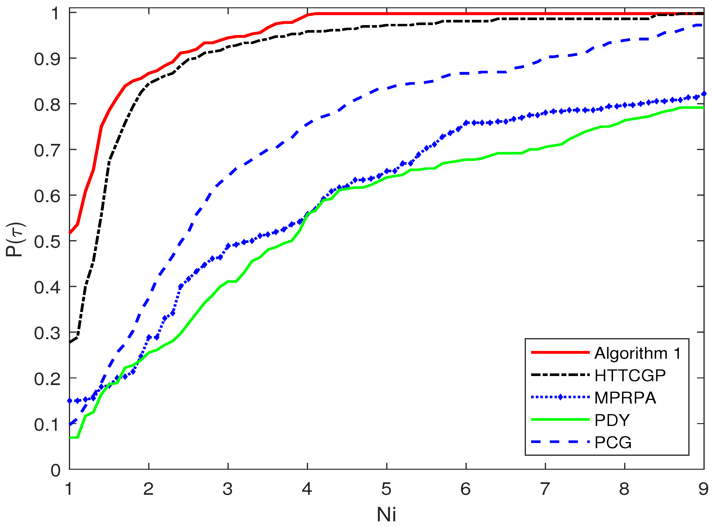
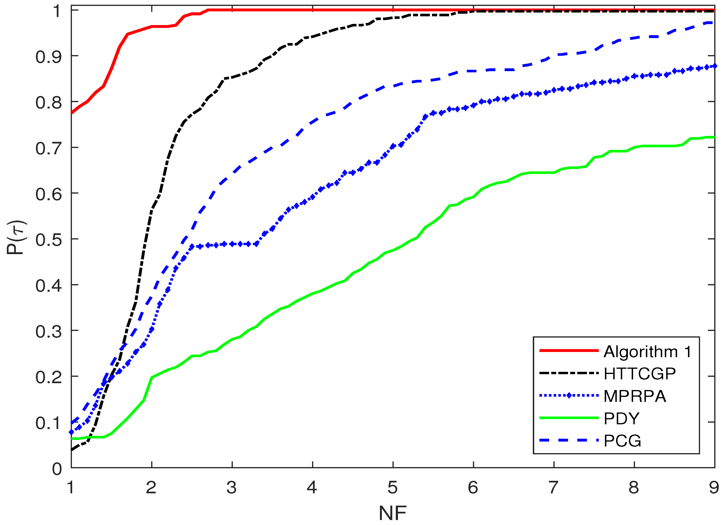
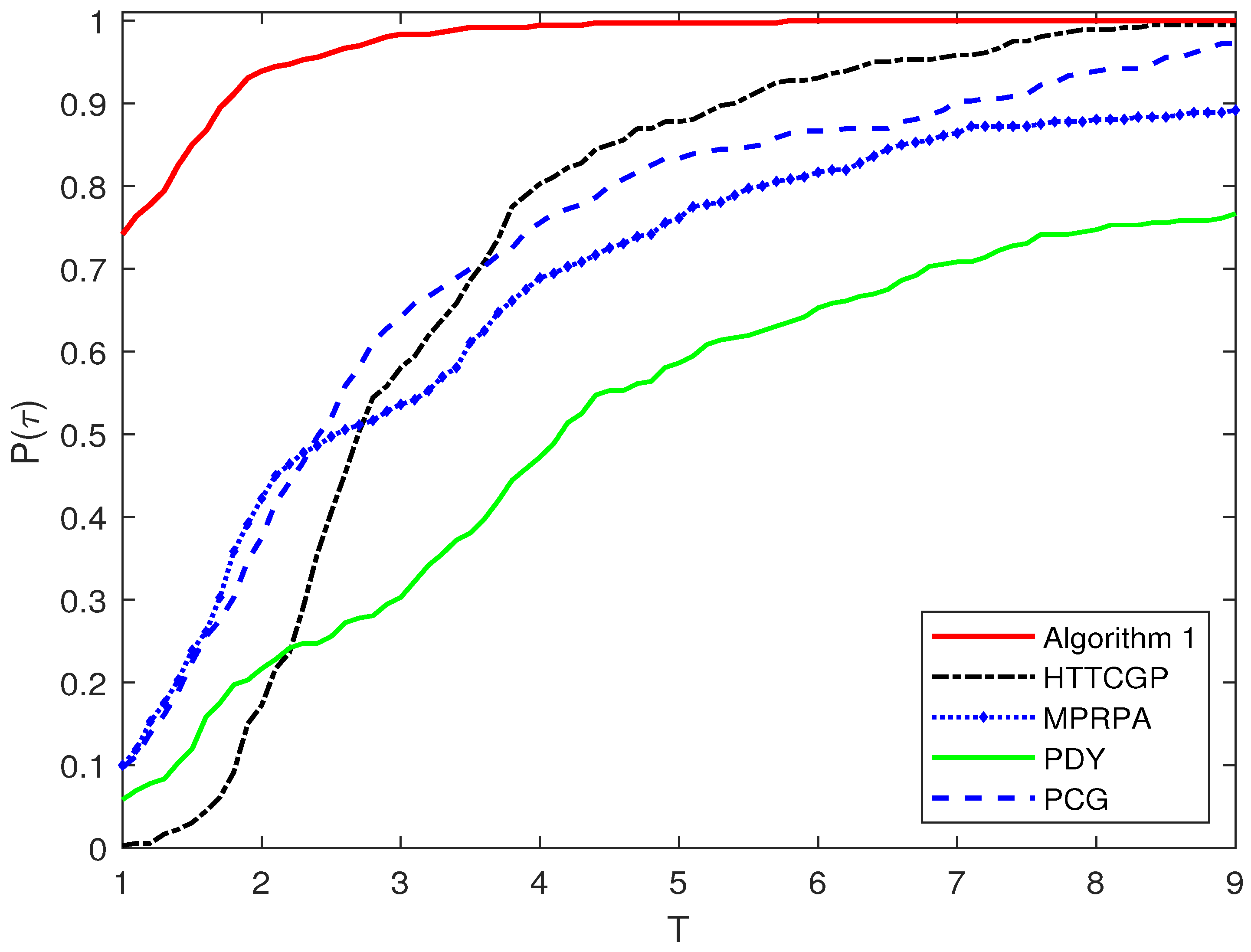
The performance profiles proposed by Dolan and Moré [33] are used to compare the numerical performance of the test methods in terms of Ni, NF, and T, respectively. We explain the performance profile by taking the number of iterations as an example. Denote the test set and the set of algorithms by P and A, respectively. We assume that we have $n_a$ algorithms and $n_p$ problems. For each problem with $p\in P$ and algorithm $a\in A$, $t_{p,a}$ represents the number of iterations required to solve problem p by algorithm a. We use the performance ratio

$$r_{p,a}=\frac{t_{p,a}}{min\left\{t_{p,a}|a\in A\right\}}$$

to compare the performance on problem p by solver a with the best performance by any algorithm on this problem. To obtain an overall assessment of the performance of the algorithm, we define

$${\rho }_a\left(\tau \right)=\frac{1}{n_p}size\left\{p\in P|r_{p,a}\le \tau \right\},$$

which is the probability for algorithm $a\in A$ that a performance ratio $r_{p,a}$ is within a factor ${\tau }_a\in \mathbb{R}$ of the best possible ratio and reflects the numerical performance of algorithm a relative to the other test algorithms in A. Obviously, algorithms with large probability $p_a\left(\tau \right)$ are to be preferred. Therefore, in the figure plotted with these ${\rho }_a\left(\tau \right)$ of the test methods, the higher the curve is, the better the corresponding algorithm a performs.

As shown in Figure 1, we observe that, in terms of the number of iterations, Algorithm 1 is the best, followed by the HTTCGP, MPRPA, and PCG methods, and the PDY method is the worst. Figure 2 indicates that Algorithm 1 has significant improvement over the other four test methods in terms of the number of function calculations, since it successfully solves about 78% of test problems with the least number of function calculations, while the percentages of the other four methods are all less than 10%. As for the reason for the significant improvement in terms of NF, it is due to the fact that the search direction of Algorithm 1 is generated by minimizing the quadratic approximate model in the two-dimensional subspace ${\mathsf{\Omega }}_k=\mathrm{Span}\{{\widehat{d}}_{k-1},g_k\},$ which implies that the search direction has new parameters corresponding to $F_k$ and thus results in that it requires less function calculations in Step 2. This is also the advantage of the SMCG methods compared with other CG methods. We can see from Figure 3 that Algorithm 1 is much faster than the other four test methods.

Figure 1. Performance profilesof the five algorithms with respect to number of iterations (Ni).

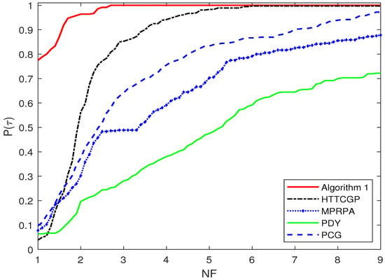
Figure 2. Performance profiles of the five algorithms with respect to number of function evaluations (NF).

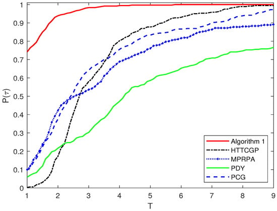
Figure 3. Performance profiles of the five algorithms with respect to CPU time (T).

The numerical experiment indicates Algorithm 1 is superior to the the other four test methods.

5. Conclusions

In this paper, an efficient SMCG method is presented for solving nonlinear monotone equations with convex constraints. The sufficient descent property of the search direction is analyzed, and the global convergence and convergence rate of the proposed algorithm are established under suitable assumptions. The numerical results confirm the effectiveness of the proposed method.

The SMCG method has illustrated a good numerical performance for solving nonlinear monotone equations with convex constraints. There is a wide research gap with regard to studying the SMCG methods for solving nonlinear monotone equations with convex constraints, including exploiting suitable quadratic or non-quadratic approximate models to derive new search directions. This is also our future research focus.

References

- Guo, D.S.; Nie, Z.Y.; Yan, L.C. The application of noise-tolerant ZD design formula to robots’ kinematic control via time-varying nonlinear equations solving. IEEE Trans. Syst. Man Cybern. Syst. 2017, 48, 2188–2197. [Google Scholar] [CrossRef]
- Shi, Y.; Zhang, Y. New discrete-time models of zeroing neural network solving systems of time-variant linear and nonlinear inequalities. IEEE Trans. Syst. Man Cybern. Syst. 2017, 50, 565–576. [Google Scholar] [CrossRef]
- Dirkse, S.P.; Ferris, M.C. MCPLIB: A collection of nonlinear mixed complementarity problems. Optim. Methods Softw. 1995, 5, 319–345. [Google Scholar] [CrossRef]
- Xiao, Y.H.; Wang, Q.Y.; Hu, Q.J. Non-smooth equations based methods for l1-norm problems with applications to compressed sensing. Nonlinear Anal. 2011, 74, 3570–3577. [Google Scholar] [CrossRef]
- Yuan, Y.X. Subspace methods for large scale nonlinear equations and nonlinear least squares. Optim. Eng. 2009, 10, 207–218. [Google Scholar] [CrossRef]
- Ahmad, F.; Tohidi, E.; Carrasco, J.A. A parameterized multi-step Newton method for solving systems of nonlinear equations. Numer. Algorithms 2016, 71, 631–653. [Google Scholar] [CrossRef]
- Lukšan, L.; Vlček, J. New quasi-Newton method for solving systems of nonlinear equations. Appl. Math. 2017, 62, 121–134. [Google Scholar] [CrossRef]
- Yu, Z. On the global convergence of a Levenberg-Marquardt method for constrained nonlinear equations. JAMC 2004, 16, 183–194. [Google Scholar] [CrossRef]
- Zhang, J.L.; Wang, Y. A new trust region method for nonlinear equations. Math. Methods Oper. Res. 2003, 58, 283–298. [Google Scholar] [CrossRef]
- Solodov, M.V.; Svaiter, B.F. A globally convergent inexact Newton method for systems of monotone equations. In Reformulation: Nonsmooth, Piecewise Smooth, Semismooth and Smoothing Methods; Fukushima, M., Qi, L., Eds.; Kluwer Academic: Boston, MA, USA, 1998; pp. 355–369. [Google Scholar]
- Zheng, Y.; Zheng, B. Two new Dai–Liao-type conjugate gradient methods for unconstrained optimization problems. J. Optim. Theory Appl. 2017, 175, 502–509. [Google Scholar] [CrossRef]
- Li, M.; Liu, H.W.; Liu, Z.X. A new family of conjugate gradient methods for unconstrained optimization. J. Appl. Math. Comput. 2018, 58, 219–234. [Google Scholar] [CrossRef]
- Xiao, Y.H.; Zhu, H. A conjugate gradient method to solve convex constrained monotone equations with applications in compressive sensing. J. Math. Anal. Appl. 2013, 405, 310–319. [Google Scholar] [CrossRef]
- Hager, H.H.; Zhang, H. A new conjugate gradient method with guaranteed descent and an efficient line search. SIAM J. Optim. 2005, 16, 170–192. [Google Scholar] [CrossRef]
- Liu, J.K.; Li, S.J. A projection method for convex constrained monotone nonlinear equations with applications. Comput. Math. Appl. 2015, 70, 2442–2453. [Google Scholar] [CrossRef]
- Dai, Y.H.; Yuan, Y.X. A nonlinear conjugate gradient with a strong global convergence property. SIAM J. Optim. 1999, 10, 177–182. [Google Scholar] [CrossRef]
- Liu, J.K.; Feng, Y.M. A derivative-free iterative method for nonlinear monotone equations with convex constraints. Numer. Algorithms 2019, 82, 245–262. [Google Scholar] [CrossRef]
- Gao, P.T.; He, C.J.; Liu, Y. An adaptive family of projection methods for constrained monotone nonlinear equations with applications. Appl. Math. Comput. 2019, 359, 1–16. [Google Scholar] [CrossRef]
- Bojari, S.; Eslahchi, M.R. Two families of scaled three-term conjugate gradient methods with sufficient descent property for nonconvex optimization. Numer. Algorithms 2020, 83, 901–933. [Google Scholar] [CrossRef]
- Li, Q.; Zheng, B. Scaled three-term derivative-free methods for solving large-scale nonlinear monotone equations. Numer. Algorithms 2021, 87, 1343–1367. [Google Scholar] [CrossRef]
- Waziri, M.Y.; Ahmed, K. Two Descent Dai-Yuan Conjugate Gradient Methods for Systems of Monotone Nonlinear Equations. J. Sci. Comput. 2022, 90, 36. [Google Scholar] [CrossRef]
- Ibrahim, A.H.; Alshahrani, M.; Al-Homidan, S. Two classes of spectral three-term derivative-free method for solving nonlinear equations with application. Numer. Algorithms 2023. [Google Scholar] [CrossRef]
- Yuan, Y.X.; Stoer, J. A subspace study on conjugate gradient algorithms. Z. Angew. Math. Mech. 1995, 75, 69–77. [Google Scholar] [CrossRef]
- Dai, Y.H.; Kou, C.X. A Barzilai-Borwein conjugate gradient method. Sci. China Math. 2016, 59, 1511–1524. [Google Scholar] [CrossRef]
- Liu, H.W.; Liu, Z.X. An efficient Barzilai–Borwein conjugate gradient method for unconstrained optimization. J. Optim. Theory Appl. 2019, 180, 879–906. [Google Scholar] [CrossRef]
- Li, Y.F.; Liu, Z.X.; Liu, H.W. A subspace minimization conjugate gradient method based on conic model for unconstrained optimization. Comput. Appl. Math. 2019, 38, 16. [Google Scholar] [CrossRef]
- Zhao, T.; Liu, H.W.; Liu, Z.X. New subspace minimization conjugate gradient methods based on regularization model for unconstrained optimization. Numer. Algorithms 2021, 87, 1501–1534. [Google Scholar] [CrossRef]
- Wang, T.; Liu, Z.; Liu, H. A new subspace minimization conjugate gradient method based on tensor model for unconstrained optimization. Int. J. Comput. Math. 2019, 96, 1924–1942. [Google Scholar] [CrossRef]
- Ortega, J.M.; Rheinboldt, W.C. Iterative Solution of Nonlinear Equation in Several Variables; Academic Press: New York, NY, USA; London, UK, 1970. [Google Scholar]
- Yin, J.H.; Jian, J.B.; Jiang, X.Z.; Liu, M. X; Wang, L.Z. A hybrid three-term conjugate gradient projection method for constrained nonlinear monotone equations with applications. Numer. Algorithms 2021, 88, 389–418. [Google Scholar] [CrossRef]
- Ou, Y.G.; Li, J.Y. A new derivative-free SCG-type projection method for nonlinear monotone equations with convex constraints. J. Appl. Math. Comput. 2018, 56, 195–216. [Google Scholar] [CrossRef]
- Ma, G.D.; Jin, J.C.; Jian, J.B.; Yin, J.H.; Han, D.L. A modified inertial three-term conjugate gradient projection method for constrained nonlinear equations with applications in compressed sensing. Numer. Algorithms 2023, 92, 1621–1653. [Google Scholar] [CrossRef]
- Dolan, E.D.; More, J.J. Benchmarking optimization software with performance profiles. Math. Program 2002, 91, 201–213. [Google Scholar] [CrossRef]
Disclaimer/Publisher’s Note: The statements, opinions and data contained in all publications are solely those of the individual author(s) and contributor(s) and not of MDPI and/or the editor(s). MDPI and/or the editor(s) disclaim responsibility for any injury to people or property resulting from any ideas, methods, instructions or products referred to in the content. |
© 2024 by the authors. Licensee MDPI, Basel, Switzerland. This article is an open access article distributed under the terms and conditions of the Creative Commons Attribution (CC BY) license (https://creativecommons.org/licenses/by/4.0/).