Soliton Solution of the Nonlinear Time Fractional Equations: Comprehensive Methods to Solve Physical Models

Abstract

In this paper, we apply two different methods, namely, the $\frac{G^{\prime }}{G}$-expansion method and the $\frac{G^{\prime }}{G^2}$-expansion method to investigate the nonlinear time fractional Harry Dym equation in the Caputo sense and the symmetric regularized long wave equation in the conformable sense. The mentioned nonlinear partial differential equations (NPDEs) arise in diverse physical applications such as ion sound waves in plasma and waves on shallow water surfaces. There exist multiple wave solutions to many NPDEs and researchers are interested in analytical approaches to obtain these multiple wave solutions. The multi-exp-function method (MEFM) formulates a solution algorithm for calculating multiple wave solutions to NPDEs and at the end of paper, we apply the MEFM for calculating multiple wave solutions to the (2 + 1)-dimensional equation.

1. Introduction

The study of nonlinear physical models relies on the analysis of wave solutions for nonlinear equations. Recently, numerous and varied methods have been applied to solve NPDEs, such as the Trial equation method [1], functional variable method [2], Sine–Gordon expansion method [3], first integral method [4], and so on [5,6,7,8,9,10,11,12].

The objective of the present paper is to apply two methods, namely, the $\frac{G^{\prime }}{G}$-expansion method and the $\frac{G^{\prime }}{G^2}$-expansion method [13], to construct new solutions for the nonlinear time fractional Harry Dym (HD) equation and the symmetric regularized long wave (SRLW) equation.

The nonlinear time fractional Harry Dym equation is given by [14]

$$\begin{array}{ccc}\hfill D_t^{\alpha }u(x,t)& =& u^3(x,t)u_{xxx}(x,t),0<\alpha \le 1,\hfill \\ \hfill u(x,0)& =& {\left(a-{\displaystyle \frac{3\sqrt{b}}{2}}x\right)}^{\frac{2}{3}},\hfill \end{array}$$

(1)

where $D^{\alpha }$ is the fractional derivative of order $\alpha$ in the Caputo sense.

For $\alpha =1$, (1) reduces to the classical nonlinear Harry Dym equation

$$u_t=u^3{u}_{xxx},$$

(2)

and the exact solution of (2) is given by

$$u(x,t)={\left(a-{\displaystyle \frac{3\sqrt{b}}{2}}(x+bt)\right)}^{\frac{2}{3}}.$$

Equation (2) was presented by Harry Dym while trying to shift several results about isospectral flow to the string equation. The relation between the classical string problem and the HD, with variables springy parameter, was introduced in 1979 and the HD equation could be considered as a particular case of a broad class of NPDEs, and also the relation between Korteweg de Vries (KdV) equations and the HD equations was considered. The HD equation describes a system in which nonlinearity and dispersion are coupled together. It has an infinite number of conservation laws and does not have the Painleve property. Many authors used numerical and analytical techniques to solve the HD equation. Singh, Kumar, and Kiliman considered the HD equation by means of the homotopy perturbation Sumudu transform technique and the Adomian decomposition technique in Ref. [15] and to obtain the solution of the HD equation with approximate analysis, Saleh and Ghiasi applied the homotopy analysis technique in Ref. [16]. Mokhtari used variational iteration, power series, and direct integration to obtain exact solutions for traveling waves of the HD equation [17], and this equation was solved by Fonseca through the Lattice–Boltzmannn technique in Ref. [18]. Rawashdeh applied the fractional reduced differential transform technique to calculate the solutions to the HD equation in Ref. [19], and the q-homotopy analysis technique is used to find analytical solutions of the HD equation in Ref. [20]. Mukherij and Assabaai applied the Lie group technique to present the numerical solutions of the HD equation in Refs. [21,22], and Shunmugarajan used the homotopy analysis technique to obtain a solution that could approximate the HD equation. The homotopy perturbation technique along with the reconstruction of the variational iteration technique were applied by Khorshidi and Soltani to get the analytical solution of the HD equation in Ref. [23].

The SRLW equation is given as follows [24]:

$$D_t^{2\gamma }u+D_x^{2\gamma }u+u{D}_t^{\gamma }\left(D_x^{\gamma }u\right)+D_x^{\gamma }u{D}_t^{\gamma }u+D_t^{2\gamma }\left(D_x^{2\gamma }u\right)=0,0<\gamma ⩽1,$$

(3)

where $D^{\gamma },$ is the conformable derivative of order $\gamma .$

Equation (3) arises in diverse physical applications such as ion sound waves in plasma. For $\gamma =1,$ this equation was noted to depict space-charge waves and weekly nonlinear ion acoustic and the real part of $u(x,t)$ is related to the dimensionless fluid velocity with a decay condition.

The abovementioned methods are usually about traveling wave solutions of NPDEs. However, there are multiple wave solutions (MWSs) to many NPDEs, for instance, multi soliton solutions to several significant models such as the Harris–Benedict equation [25,26], and the KDV equation [27]. Thus, one is interested in presenting a method for obtaining MWSs to NPDEs and the MEFM formulates a solution algorithm for calculating MWSs to NPDEs.

At the end of the article, we apply the MEFM [28] for calculating MWSs to the following (2 + 1)-dimensional equation [29]

$$u_{yt}+\alpha u_{xx}+\beta u_{yy}+u_{xy}=0,\alpha ,\beta \in \mathbb{C}.$$

for the following special cases

$$u_{yt}+5u_{xx}+{(-1)}^{\frac{2}{3}}5u_{yy}+u_{xy}=0,$$

(4)

and

$$u_{yt}-5u_{xx}-5u_{yy}+u_{xy}=0.$$

(5)

We get multi classes of solutions including one, two, and triple-soliton solutions. All the computations have been performed applying the software package Maple 15. The gained solutions contain three classes of soliton wave solutions in terms of one, two, and three wave solutions, which are displayed graphically, highlighting the effects of non-linearity. Besides, the multiple soliton solutions are proposed with more arbitrary autocephalous parameters, in which the one, two, and triple solutions are localized in every direction in space. The obtained results have shown a major impact on wave behavior and can be applied in different branches of science, especially in fluid dynamics, to investigate the understanding of complex physical phenomena.

The MEFM applied by some of the powerful authors for different nonlinear equations such as the (3 + 1)-dimensional generalized KP and BKP equations [30], the nonlinear evolution equations [31], the generalized (1 + 1)-dimensional, and (2 + 1)-dimensional Ito equations [32], the new (2 + 1)-dimensional KdV equation [33], the (2 + 1)-dimensional Calogero–Bogoyavlenskii–Schiff equation [34], and a new generalization of the associated Camassa–Holm equation [35], and so on [36]. Additionally, in Ref. [33], the authors utilized the MEFM for the KdV equation, and obtained one, two, and three-soliton-type solutions with interpretations for the gained soliton solutions.

2. Algorithm for the $\frac{{\mathit{G}}^{\prime }}{{\mathit{G}}^{\mathbf{2}}}$-Expansion, the $\frac{{\mathit{G}}^{\prime }}{\mathit{G}}$-Expansion, and the Multi-Exp-Function Method

2.1. The Basic Idea of the $\frac{G^{\prime }}{G^2}$-Expansion Method

In this subsection, we consider the algorithm of the $\frac{G^{\prime }}{G^2}$-expansion method for a nonlinear fractional PDE as follows:

• Consider the general nonlinear fractional PDE of the type:

  $$\mathsf{N}(u,D_t^{\alpha }u,D_x^{\alpha }u,D_x^{\beta }u,D_x^{\alpha }{D}_x^{\beta }u,D_t^{\alpha }{D}_t^{\beta }u,\cdots )=0,0<\alpha ,\beta ⩽1,$$

  (6)

  where $u=u(x,t).$
• Convert the nonlinear PDE (6) into an ODE through the following transformation,

  $$\epsilon ={\displaystyle \frac{d{x}^{d\beta }}{\Gamma (1+\beta )}}+{\displaystyle \frac{c{x}^{c\alpha }}{\Gamma (1+\alpha )}},u(x,t)=u\left(\epsilon \right),$$

  (7)

  where d and c are constants and $\Gamma (.)$ is the Gamma function defined in Ref. [3].
• Rewrite Equation (6) as

  $$\tilde{\mathsf{N}}(u,u^{\prime },u^{″},u^{‴},\dots )=0.$$

  (8)
• Assume the general solution of (8) can be expressed in terms of $\frac{G^{\prime }}{G^2}$ as

  $$u\left(\epsilon \right)=a_0+\sum _{i=1}^N\left[a_i{\left(\frac{G^{\prime }\left(\epsilon \right)}{G^2\left(\epsilon \right)}\right)}^i+b_i{\left(\frac{G^{\prime }\left(\epsilon \right)}{G^2\left(\epsilon \right)}\right)}^{-i}\right],$$

  (9)

  where $G\left(\epsilon \right)$ satisfies the following Riccati equation:

  $${\left(\frac{G^{\prime }\left(\epsilon \right)}{G^2\left(\epsilon \right)}\right)}^{\prime }=\eta +\lambda {\left(\frac{G^{\prime }\left(\epsilon \right)}{G^2\left(\epsilon \right)}\right)}^2,$$

  (10)

  in which $\eta \ne 1,\lambda \ne 0.$ The constants $b_N$ or $a_N$ may be zero, but both of them cannot be zero simultaneously. Also, $b_i,a_i,i=1,\dots ,N,$ are constants to be determined in the next step. In addition, the value of $N\in \mathbb{N}$ can be computed through the homogeneous balance principle [37].
  Notice that (10) results in

  $$\begin{array}{ccc}& & G^{″}\left(\epsilon \right)={\displaystyle \frac{\eta G^4+{\left(G^{\prime }\right)}^2(2G+\lambda )}{G^2}},\hfill \end{array}$$

  (11)

  $$\begin{array}{ccc}& & G^{‴}\left(\epsilon \right)=G^{\prime }(6G\eta +2\lambda \eta )+{\displaystyle \frac{{\left(G^{\prime }\right)}^3}{G^2}}(6+6\lambda {\displaystyle \frac{1}{G}}+2{\lambda }^2{\displaystyle \frac{1}{G^2}}).\hfill \end{array}$$

  (12)
• Insert (9), along with (10), into (8). Collect all coefficients of the same power of ${\left(\frac{G^{\prime }\left(\epsilon \right)}{G^2\left(\epsilon \right)}\right)}^{\pm i}$ for $i=1,\dots ,N.$ Then, set all of the obtained coefficients to zero. Then solve the system of algebraic equations on variables $a_0,b_i,a_i,\eta ,\lambda ,c$ and $d,$ for $i=1,\dots ,N.$
• Depending on the values of $\eta$ and $\lambda ,$ the general solutions of (10) can be separated into the following cases:
  Case 1: $\lambda \eta >0;$

  $${\displaystyle \frac{G^{\prime }\left(\epsilon \right)}{G^2\left(\epsilon \right)}}=\sqrt{{\displaystyle \frac{\eta }{\lambda }}}\left({\displaystyle \frac{Ccos\left(\sqrt{\eta \lambda }\epsilon \right)+Dsin\left(\sqrt{\eta \lambda }\epsilon \right)}{Dcos\left(\sqrt{\eta \lambda }\epsilon \right)-Csin\left(\sqrt{\eta \lambda }\epsilon \right)}}\right),$$

  (13)
  Case 2: $\lambda \eta <0;$

  $${\displaystyle \frac{G^{\prime }\left(\epsilon \right)}{G^2\left(\epsilon \right)}}=-{\displaystyle \frac{\sqrt{\left|\eta \lambda \right|}}{\lambda }}\left({\displaystyle \frac{Csinh\left(2\sqrt{\left|\eta \lambda \right|}\epsilon \right)+Ccosh\left(2\sqrt{\left|\eta \lambda \right|}\epsilon \right)+D}{Csinh\left(2\sqrt{\left|\eta \lambda \right|}\epsilon \right)+Ccosh\left(2\sqrt{\left|\eta \lambda \right|}\epsilon \right)-D}}\right),$$

  (14)
  Case 3: $\lambda \ne 0,\eta =0;$

  $${\displaystyle \frac{G^{\prime }\left(\epsilon \right)}{G^2\left(\epsilon \right)}}=-{\displaystyle \frac{C}{\lambda (C\epsilon +D)}},$$

  (15)

  where $C,D\ne 0.$
• By substituting the obtained values of $a_0,b_i,a_i,\eta ,\lambda ,c,d$ and the solutions (13)–(15) into (9) with the transformation (7), the exact traveling wave solutions of (6) can be obtained.

2.2. The Basic Idea of the $\frac{G^{\prime }}{G}$-Expansion Method

In this subsection, we present the algorithm of the $\frac{G^{\prime }}{G}$-expansion method for a nonlinear fractional PDE as follows:

• Consider the general nonlinear fractional PDE of the type (6).
• Convert the nonlinear PDE (6) into an ODE through the transformation defined in (7).
• Rewrite (6) as the NODE (8).
• Assume the general solution of (8) can be expressed in terms of $\frac{G^{\prime }}{G}$ as

  $$u\left(\epsilon \right)=\sum _{i=0}^N\left[a_i{\left(\frac{G^{\prime }\left(\epsilon \right)}{G\left(\epsilon \right)}\right)}^i\right],$$

  (16)

  where $G\left(\epsilon \right)$ satisfies the following second order ODE:

  $$G^{″}\left(\epsilon \right)+\lambda G^{\prime }\left(\epsilon \right)+\eta G\left(\epsilon \right)=0,$$

  (17)

  in which $\eta ,\lambda$ and $a_i,i=1,\cdots ,N,$ are constants to be determined later.
  Notice that we can obtain the value of N by the homogeneous balance principle.
• Insert (16), along with (17), into (8). Collect all coefficients of the same power of ${\left(\frac{G^{\prime }\left(\epsilon \right)}{G\left(\epsilon \right)}\right)}^i.$ Then set all of the obtained coefficients to zero. Then solve the system of algebraic equations on variables $a_i,\eta ,\lambda ,c$.
• Depending on the values of $\eta$ and $\lambda ,$ the general solutions of (17) can be separated into the following cases:
  Case 1: ${\lambda }^2-4\eta >0;$

  $${\displaystyle \frac{G^{\prime }\left(\epsilon \right)}{G\left(\epsilon \right)}}=0.5\sqrt{{\lambda }^2-4\eta }\left({\displaystyle \frac{Ccosh\left(0.5\sqrt{{\lambda }^2-4\eta }\epsilon \right)+Dsinh\left(0.5\sqrt{{\lambda }^2-4\eta }\epsilon \right)}{Csinh\left(0.5\sqrt{{\lambda }^2-4\eta }\epsilon \right)+Dcosh\left(0.5\sqrt{{\lambda }^2-4\eta }\epsilon \right)}}\right),$$

  (18)
  Case 2: ${\lambda }^2-4\eta <0;$

  $${\displaystyle \frac{G^{\prime }\left(\epsilon \right)}{G\left(\epsilon \right)}}=0.5\sqrt{{\lambda }^2-4\eta }\left({\displaystyle \frac{-Csin\left(0.5\sqrt{-{\lambda }^2+4\eta }\epsilon \right)+Dcos\left(0.5\sqrt{-{\lambda }^2+4\eta }\epsilon \right)}{Ccos\left(0.5\sqrt{-{\lambda }^2+4\eta }\epsilon \right)+Dsin\left(0.5\sqrt{-{\lambda }^2+4\eta }\epsilon \right)}}\right),$$

  (19)
  Case 3: ${\lambda }^2-4\eta =0;$

  $${\displaystyle \frac{G^{\prime }\left(\epsilon \right)}{G\left(\epsilon \right)}}={\displaystyle \frac{D}{D\epsilon +C}}-{\displaystyle \frac{\lambda }{2}},$$

  (20)

  where $C,D\ne 0.$
• By substituting the obtained values of $a_i,\eta ,\lambda ,c$ and the solutions (18), (19), and (78) into (16) with the transformation (7), the exact traveling wave solutions of (6) can be obtained.

2.3. The Basic Idea of the Multi-Exp-Function Method

In this subsection, we formulate the MEFM by considering

$$\mathsf{N}(x,t,u_t,u_x,\dots )=0,$$

(21)

where $u=u(x,t).$

• Step 1: Assume that

  $${\epsilon }_i=c_i{e}^{{\epsilon }_i},{\epsilon }_i=S_{i}x-{\omega }_{i}t,{\epsilon }_i=k_{i}x-{\omega }_{i}t,i\in [1,n],$$

  (22)

  in which $k_i$, $c_i,$ and ${\omega }_i$ are angular wave numbers, arbitrary constants, and wave frequencies, respectively. Notice that

  $${\epsilon }_{i,x}=k_i{\epsilon }_i,{\epsilon }_{i,t}=-{\omega }_i{\epsilon }_i,i\in [1,n].$$

  (23)
• Step 2: Assume

  $$\begin{array}{c}u(x,t):={\displaystyle \frac{\mathcal{K}({\epsilon }_1,{\epsilon }_2,\cdots ,{\epsilon }_n)}{\mathcal{H}({\epsilon }_1,{\epsilon }_2,\cdots ,{\epsilon }_n)}},\hfill \\ {\displaystyle \mathcal{K}:=\sum _{r,s=1}^n\sum _{i,j=0}^M{P}_{rs,ij}{\epsilon }_r^i{\epsilon }_s^j,}\hfill \\ {\displaystyle \mathcal{H}:=\sum _{r,s=1}^n\sum _{i,j=0}^N{Q}_{rs,ij}{\epsilon }_r^i{\epsilon }_s^j,}\hfill \end{array}$$

  (24)

  where $Q_{rs,ij}$ and $P_{rs,ij}$ are fixed to be determined from (21).
  We now get

  $$\tilde{\mathsf{N}}(x,t,{\epsilon }_1,{\epsilon }_2,\cdots ,{\epsilon }_n)=0.$$

  (25)
• Step 3: When we solve a system of algebraic equations on variables $w_i,$ $k_i,$ $Q_{rs,ij}$ and $P_{rs,ij}$, we get the MWSs u as

  $$u(x,t)={\displaystyle \frac{\mathcal{K}(c_{1}exp(k_{1}x-{\omega }_{1}t),\cdots ,c_{n}exp(k_{n}x-{\omega }_{n}t))}{\mathcal{H}(c_{1}exp(k_{1}x-{\omega }_{1}t),\cdots ,c_{n}exp(k_{n}x-{\omega }_{n}t))}}.$$

  (26)

3. Application of the $\frac{{\mathit{G}}^{\prime }}{{\mathit{G}}^{\mathbf{2}}}$-Expansion Method

Example 1.

Assume the nonlinear time fractional Harry Dym Equation (1). where $D^{\alpha }$ is the fractional derivative of order α in the Caputo sense and for a given function $f:{\mathbb{R}}^{+}⟶\mathbb{R}$ is defined by

$$D^{\alpha }f\left(t\right)=I^{n-\alpha }{D}^{n}f\left(t\right)={\displaystyle \frac{1}{\Gamma (n-\alpha )}}{\int }_0^t{\displaystyle \frac{f^{\left(n\right)}\left(s\right)}{{(t-s)}^{\alpha -n+1}}}ds,n-1<\alpha <n\in \mathbb{N},t>0,$$

and the Riemann–Liouville fractional integral operator $I_t^{\beta }$ of order β is defined by

$$I_t^{\beta }f\left(t\right)={\displaystyle \frac{1}{\Gamma \left(\beta \right)}}{\int }_0^t{(t-s)}^{\beta -1}f\left(s\right)ds,\beta >0,t>0.$$

Now, we employ the following transformations, which represents a new dependent variable

$$\begin{array}{c}{\displaystyle X={\int }_{-\infty }^x{\displaystyle \frac{ds}{u(s,t)}},}\hfill \\ T=-{\displaystyle \frac{t^{\alpha }}{\Gamma (1+\alpha )}},\hfill \\ \Xi (X,T)=u\left(x(X,T),t(X,T)\right)\hfill \end{array}$$

(27)

where $x=x(X,T)$ and $t=t(X,T).$

We shall employ the fact that $u(x,t)$ and its spatial derivative tends to zero as $\left|x\right|\to \infty .$ Then

$$\begin{array}{ccc}\hfill {\displaystyle \frac{{\partial }^{\alpha }}{\partial t^{\alpha }}}& =& {\displaystyle \frac{\partial }{\partial X}}{\displaystyle \frac{{\partial }^{\alpha }X}{\partial t^{\alpha }}}+{\displaystyle \frac{\partial }{\partial T}}{\displaystyle \frac{{\partial }^{\alpha }T}{\partial t^{\alpha }}}\hfill \\ & =& -{\displaystyle \frac{\partial }{\partial T}}-\left({\displaystyle \frac{\Xi {\Xi }_{XX}-\frac{3}{2}{\Xi }_X^2}{{\Xi }^2}}\right){\displaystyle \frac{\partial }{\partial X}}.\hfill \end{array}$$

Also,

$${\displaystyle \frac{\partial }{\partial x}}={\displaystyle \frac{1}{\Xi (X,T)}}{\displaystyle \frac{\partial }{\partial X}}.$$

Therefore, (1) can be expressed as

$${\Xi }_T+{\displaystyle \frac{{\Xi }_{XXX}{\Xi }^2-3{\Xi }_{XX}{\Xi }_X\Xi +\frac{3}{2}{\Xi }_X^3}{{\Xi }^2}}=0.$$

(28)

Now consider the following transformation

$$\psi (X,T)={\displaystyle \frac{{\Xi }_X}{\Xi }}.$$

(29)

From (28) and (30), we get the following KdV equation

$${\psi }_T-{\displaystyle \frac{3}{2}}{\psi }^2{\psi }_X+{\psi }_{XXX}=0.$$

(30)

Now, let

$$\begin{array}{c}\psi (X,T)=\psi \left(\epsilon \right),\hfill \\ \epsilon =\epsilon (X,T)=X-cT,\hfill \end{array}$$

(31)

where c is constant.

Inserting (31) in (30), we get

$$-c{\psi }^{\prime }-{\displaystyle \frac{3}{2}}{\psi }^2{\psi }^{\prime }+{\psi }^{‴}=0.$$

(32)

Integration of (32) yields

$$-c\psi -{\displaystyle \frac{1}{2}}{\psi }^3+{\psi }^{″}=0.$$

(33)

Here, we get the balancing number $3N=N+2$ or $N=1.$

Suppose the solution of (33) can be given by

$$\psi \left(\epsilon \right)=a_0+a_1\left({\displaystyle \frac{G^{\prime }}{G^2}}\right)+b_1{\left({\displaystyle \frac{G^{\prime }}{G^2}}\right)}^{-1},$$

(34)

in which $a_0,b_1,a_1$ are constant to be determined later.

Inserting Equation (34) into Equation (33), we have

$$\begin{array}{ccc}& & -c{a}_0-c{a}_1\frac{G^{\prime }\left(\epsilon \right)}{G^2\left(\epsilon \right)}-c{b}_1\frac{G^2\left(\epsilon \right)}{G^{\prime }\left(\epsilon \right)}-\frac{1}{2}{a}_0^3-\frac{3}{2}{a}_0^2{a}_1\frac{G\left(\epsilon \right)}{G^2\left(\epsilon \right)}-\frac{3}{2}{a}_0^2{b}_1\frac{G^2\left(\epsilon \right)}{G^{\prime }\left(\epsilon \right)}-\frac{3}{2}{a}_0{a}_1^2\frac{{\left(G^{\prime }\left(\epsilon \right)\right)}^2}{G^4\left(\epsilon \right)}\hfill \\ & & -3a_0{a}_1{b}_1-\frac{3}{2}{a}_0{b}_1^2\frac{G^4\left(\epsilon \right)}{{\left(G^{\prime }\left(\epsilon \right)\right)}^2}-\frac{1}{2}{a}_1^3\frac{{\left(G^{\prime }\left(\epsilon \right)\right)}^3}{G^6\left(\epsilon \right)}-\frac{3}{2}{a}_1^2{b}_1\frac{G^{\prime }\left(\epsilon \right)}{G^2\left(\epsilon \right)}-\frac{3}{2}{a}_1{b}_1^2\frac{G^2\left(\epsilon \right)}{G^{\prime }\left(\epsilon \right)}-\frac{1}{2}\frac{b_1^3{G}^6\left(\epsilon \right)}{{\left(G^{\prime }\left(\epsilon \right)\right)}^3}\hfill \\ & & +a_1\frac{G^{‴}\left(\epsilon \right)}{G^2\left(\epsilon \right)}-6a_1\frac{G^{″}\left(\epsilon \right)G^{\prime }\left(\epsilon \right)}{G^3\left(\epsilon \right)}+6a_1\frac{{\left(G^{\prime }\left(\epsilon \right)\right)}^3}{G^4\left(\epsilon \right)}+2b_1\frac{G^2\left(\epsilon \right)G^{″}\left(\epsilon \right)}{{\left(G^{\prime }\left(\epsilon \right)\right)}^3}-2b_1\frac{G\left(\epsilon \right)G^{″}\left(\epsilon \right)}{G^{\prime }\left(\epsilon \right)}\hfill \\ & & -b_1\frac{G^2\left(\epsilon \right)G^{‴}\left(\epsilon \right)}{{\left(G^{\prime }\left(\epsilon \right)\right)}^2}+2b_1{G}^{\prime }\left(\epsilon \right)=0.\hfill \end{array}$$

Note 1.

Making use of (10), we get

$$G^{″}\left(\epsilon \right)=\frac{\eta G^4\left(\epsilon \right)+2{\left(G^{\prime }\left(\epsilon \right)\right)}^{2}G\left(\epsilon \right)+\lambda {\left(G^{\prime }\left(\epsilon \right)\right)}^2}{G^2\left(\epsilon \right)},$$

(35)

 and 

$$G^{‴}\left(\epsilon \right)=6\eta G\left(\epsilon \right)G^{\prime }\left(\epsilon \right)+6\frac{{\left(G^{\prime }\left(\epsilon \right)\right)}^3}{G^2\left(\epsilon \right)}+6\lambda \frac{{\left(G^{\prime }\left(\epsilon \right)\right)}^3}{G^3\left(\epsilon \right)}+2\lambda \eta G^{\prime }\left(\epsilon \right)+2{\lambda }^2\frac{{\left(G^{\prime }\left(\epsilon \right)\right)}^3}{G^4\left(\epsilon \right)}.$$

(36)

Using (10), (35), and (36), and then inserting ${\displaystyle \frac{G^{\prime }}{G^2}}:=X,$ and ${\left({\displaystyle \frac{G^{\prime }}{G^2}}\right)}^{-1}:=Y,$ we have that 

$$\begin{array}{c}{\displaystyle -c{a}_{1}X-c{b}_{1}Y-\frac{3}{2}{a}_0^2{a}_{1}X-\frac{3}{2}{a}_0^2{b}_{1}Y-\frac{3}{2}{a}_0{a}_1^2{X}^2-\frac{3}{2}{a}_0{b}_1^2{Y}^2-\frac{3}{2}{a}_1^2{b}_{1}X-\frac{3}{2}{a}_1{b}_1^{2}Y}\hfill \\ {\displaystyle +2a_1\lambda \eta X+2b_1\eta \lambda Y+2a_1{\lambda }^2{X}^3+2b_1{\eta }^2{Y}^3-\frac{1}{2}{a}_1^3{X}^3-3a_0{a}_1{b}_1-\frac{1}{2}{b}_1^3{Y}^3-\frac{1}{2}{a}_0^3-c{a}_0=0.}\hfill \end{array}$$

By collecting all terms with the same power of X and Y and then equating each coefficients of this polynomial to zero, we get the following system of algebraic equations:

$$\begin{array}{ccc}& & Y^3:2b_1{\eta }^2-\frac{1}{2}{b}_1^3=0,\hfill \\ & & Y^2:-\frac{3}{2}{a}_0{b}_1^2=0,\hfill \\ & & Y:-c{b}_1-\frac{3}{2}{a}_0^2{b}_1-\frac{3}{2}{a}_1{b}_1^2+2b_1\eta \lambda =0,\hfill \\ & & X^0{Y}^0:-3a_1{a}_0{b}_1-\frac{1}{2}{a}_0^3-c{a}_0=0,\hfill \\ & & X:-c{a}_1-\frac{3}{2}{a}_0^2{a}_1-\frac{3}{2}{a}_1^2{b}_1+2a_1\lambda \eta =0,\hfill \\ & & X^2:-\frac{3}{2}{a}_0{a}_1^2=0,\hfill \\ & & X^3:2a_1{\lambda }^2-\frac{1}{2}{a}_1^3=0.\hfill \end{array}$$

Solving the above system of nonlinear algebraic equation, we get

$$\begin{array}{ccc}& & c=-\frac{1}{2}{a}_0^2,\eta =\eta ,\lambda =\lambda ,a_0=a_0,a_1=0,b_1=0,\hfill \end{array}$$

(37)

$$\begin{array}{ccc}& & c=c,\eta =\eta ,\lambda =\lambda ,a_0=0,a_1=0,b_1=0,\hfill \end{array}$$

(38)

$$\begin{array}{ccc}& & c=2\lambda \eta ,\eta =\eta ,\lambda =\lambda ,a_0=0,a_1=0,b_1=2\eta ,\hfill \end{array}$$

(39)

$$\begin{array}{ccc}& & c=2\lambda \eta ,\eta =\eta ,\lambda =\lambda ,a_0=0,a_1=0,b_1=-2\eta ,\hfill \end{array}$$

(40)

$$\begin{array}{ccc}& & c=2\lambda \eta ,\eta =\eta ,\lambda =\lambda ,a_0=0,a_1=2\lambda ,b_1=0,\hfill \end{array}$$

(41)

$$\begin{array}{ccc}& & c=2\lambda \eta ,\eta =\eta ,\lambda =\lambda ,a_0=0,a_1=-2\lambda ,b_1=0,\hfill \end{array}$$

(42)

$$\begin{array}{ccc}& & c=-4\lambda \eta ,\eta =\eta ,\lambda =\lambda ,a_0=0,a_1=2\lambda ,b_1=2\eta ,\hfill \end{array}$$

(43)

$$\begin{array}{ccc}& & c=8\lambda \eta ,\eta =\eta ,\lambda =\lambda ,a_0=0,a_1=-2\lambda ,b_1=2\eta ,\hfill \end{array}$$

(44)

$$\begin{array}{ccc}& & c=8\lambda \eta ,\eta =\eta ,\lambda =\lambda ,a_0=0,a_1=2\lambda ,b_1=-2\eta ,\hfill \end{array}$$

(45)

$$\begin{array}{ccc}& & c=-4\lambda \eta ,\eta =\eta ,\lambda =\lambda ,a_0=0,a_1=-2\lambda ,b_1=-2\eta .\hfill \end{array}$$

(46)

Inserting (43) and (46) in (34), we get

$$\psi \left(\epsilon \right)=\pm 2\lambda \left({\displaystyle \frac{G^{\prime }}{G^2}}\right)\pm 2\eta {\left({\displaystyle \frac{G^{\prime }}{G^2}}\right)}^{-1}.$$

(47)

Therefore, we get three types of travelling wave solutions as follows:

• if $\lambda \eta >0;$

  $$u_{1,2}(x,t)=\pm 2\lambda {\xi }_1\pm 2\eta {\left({\xi }_1\right)}^{-1},$$

  (48)

  in which

  $${\xi }_1:=\sqrt{{\displaystyle \frac{\eta }{\lambda }}}\left({\displaystyle \frac{Ccos(\sqrt{\eta \lambda }(x-\frac{-4\lambda \eta t^{\alpha }}{\Gamma (1+\alpha )})+Dsin\left(\sqrt{\eta \lambda }(x-\frac{-4\lambda \eta t^{\alpha }}{\Gamma (1+\alpha )})\right)}{Dcos\left(\sqrt{\eta \lambda }(x-\frac{-4\lambda \eta t^{\alpha }}{\Gamma (1+\alpha )})\right)-Csin\left(\sqrt{\eta \lambda }(x-\frac{-4\lambda \eta t^{\alpha }}{\Gamma (1+\alpha )})\right)}}\right),$$
• if $\lambda \eta <0;$

  $$u_{1,2}(x,t)=\pm 2\lambda {\xi }_2\pm 2\eta {\left({\xi }_2\right)}^{-1},$$

  (49)

  in which

  $$\begin{array}{c}\hfill {\xi }_2:=-{\displaystyle \frac{\sqrt{\left|\eta \lambda \right|}}{\lambda }}\left({\displaystyle \frac{Csinh\left(2\sqrt{\left|\eta \lambda \right|}(x-\frac{-4\lambda \eta t^{\alpha }}{\Gamma (1+\alpha )})\right)+Ccosh\left(2\sqrt{\left|\eta \lambda \right|}(x-\frac{-4\lambda \eta t^{\alpha }}{\Gamma (1+\alpha )})\right)+D}{Csinh\left(2\sqrt{\left|\eta \lambda \right|}(x-\frac{-4\lambda \eta t^{\alpha }}{\Gamma (1+\alpha )})\right)+Ccosh\left(2\sqrt{\left|\eta \lambda \right|}(x-\frac{-4\lambda \eta t^{\alpha }}{\Gamma (1+\alpha )})\right)-D}}\right),\end{array}$$
• if $\lambda \ne 0,\eta =0;$

  $$u_{1,2}(x,t)=\pm 2\lambda {\xi }_3\pm 2\eta {\left({\xi }_3\right)}^{-1},$$

  in which

  $${\xi }_3:=-{\displaystyle \frac{C}{\lambda (C(x-\frac{-4\lambda \eta t^{\alpha }}{\Gamma (1+\alpha )})+D)}},$$

  where $C,D\ne 0.$

Inserting (44) and (45) in (34), we get

$$\begin{array}{c}\hfill \psi \left(\epsilon \right)=\pm 2\lambda \left({\displaystyle \frac{G^{\prime }}{G^2}}\right)\mp 2\eta {\left({\displaystyle \frac{G^{\prime }}{G^2}}\right)}^{-1}.\end{array}$$

(50)

Therefore, we get three types of travelling wave solutions as follows:

• if $\lambda \eta >0;$

  $$u_{3,4}(x,t)=\pm 2\lambda {\xi }_1\mp 2\eta {\left({\xi }_1\right)}^{-1},$$

  (51)

  in which

  $${\xi }_1:=\sqrt{{\displaystyle \frac{\eta }{\lambda }}}\left({\displaystyle \frac{Ccos(\sqrt{\eta \lambda }(x-\frac{8\lambda \eta t^{\alpha }}{\Gamma (1+\alpha )})+Dsin\left(\sqrt{\eta \lambda }(x-\frac{8\lambda \eta t^{\alpha }}{\Gamma (1+\alpha )})\right)}{Dcos\left(\sqrt{\eta \lambda }(x-\frac{8\lambda \eta t^{\alpha }}{\Gamma (1+\alpha )})\right)-Csin\left(\sqrt{\eta \lambda }(x-\frac{8\lambda \eta t^{\alpha }}{\Gamma (1+\alpha )})\right)}}\right),$$
• if $\lambda \eta <0;$

  $$u_{3,4}(x,t)=\pm 2\lambda {\xi }_2\mp 2\eta {\left({\xi }_2\right)}^{-1},$$

  (52)

  in which

  $${\xi }_2:=-{\displaystyle \frac{\sqrt{\left|\eta \lambda \right|}}{\lambda }}\left({\displaystyle \frac{Csinh\left(2\sqrt{\left|\eta \lambda \right|}(x-\frac{8\lambda \eta t^{\alpha }}{\Gamma (1+\alpha )})\right)+Ccosh\left(2\sqrt{\left|\eta \lambda \right|}(x-\frac{8\lambda \eta t^{\alpha }}{\Gamma (1+\alpha )})\right)+D}{Csinh\left(2\sqrt{\left|\eta \lambda \right|}(x-\frac{8\lambda \eta t^{\alpha }}{\Gamma (1+\alpha )})\right)+Ccosh\left(2\sqrt{\left|\eta \lambda \right|}(x-\frac{8\lambda \eta t^{\alpha }}{\Gamma (1+\alpha )})\right)-D}}\right),$$
• if $\lambda \ne 0,\eta =0;$

  $$u_{3,4}(x,t)=\pm 2\lambda {\xi }_3\mp 2\eta {\left({\xi }_3\right)}^{-1},$$

  in which

  $${\xi }_3:=-{\displaystyle \frac{C}{\lambda (C(x-\frac{8\lambda \eta t^{\alpha }}{\Gamma (1+\alpha )})+D)}},$$

  where $C,D\ne 0.$

Inserting (41) and (42) in (34), we get

$$\psi \left(\epsilon \right)=\pm 2\lambda \left({\displaystyle \frac{G^{\prime }}{G^2}}\right).$$

(53)

Therefore, we get three types of travelling wave solutions as follows:

• if $\lambda \eta >0;$

  $$u_{5,6}(x,t)=\pm 2\lambda {\xi }_1,$$

  (54)

  in which

  $${\xi }_1:=\sqrt{{\displaystyle \frac{\eta }{\lambda }}}\left({\displaystyle \frac{Ccos(\sqrt{\eta \lambda }(x-\frac{2\lambda \eta t^{\alpha }}{\Gamma (1+\alpha )})+Dsin\left(\sqrt{\eta \lambda }(x-\frac{2\lambda \eta t^{\alpha }}{\Gamma (1+\alpha )})\right)}{Dcos\left(\sqrt{\eta \lambda }(x-\frac{2\lambda \eta t^{\alpha }}{\Gamma (1+\alpha )})\right)-Csin\left(\sqrt{\eta \lambda }(x-\frac{2\lambda \eta t^{\alpha }}{\Gamma (1+\alpha )})\right)}}\right),$$
• if $\lambda \eta <0;$

  $$\begin{array}{c}\hfill u_{5,6}(x,t)=\pm 2\lambda {\xi }_2,\end{array}$$

  (55)

  in which

  $${\xi }_2:=-{\displaystyle \frac{\sqrt{\left|\eta \lambda \right|}}{\lambda }}\left({\displaystyle \frac{Csinh\left(2\sqrt{\left|\eta \lambda \right|}(x-\frac{2\lambda \eta t^{\alpha }}{\Gamma (1+\alpha )})\right)+Ccosh\left(2\sqrt{\left|\eta \lambda \right|}(x-\frac{2\lambda \eta t^{\alpha }}{\Gamma (1+\alpha )})\right)+D}{Csinh\left(2\sqrt{\left|\eta \lambda \right|}(x-\frac{2\lambda \eta t^{\alpha }}{\Gamma (1+\alpha )})\right)+Ccosh\left(2\sqrt{\left|\eta \lambda \right|}(x-\frac{2\lambda \eta t^{\alpha }}{\Gamma (1+\alpha )})\right)-D}}\right),$$
• if $\lambda \ne 0,\eta =0;$

  $$u_{3,4}(x,t)=\pm 2\lambda {\xi }_3,$$

  in which

  $${\xi }_3:=-{\displaystyle \frac{C}{\lambda (C(x-\frac{2\lambda \eta t^{\alpha }}{\Gamma (1+\alpha )})+D)}},$$

  where $C,D\ne 0.$

Inserting (39) and (40) in (34), we get

$$\psi \left(\epsilon \right)=\mp 2\eta {\left({\displaystyle \frac{G^{\prime }}{G^2}}\right)}^{-1}.$$

(56)

Therefore, we get three types of travelling wave solutions as follows:

• if $\lambda \eta >0;$

  $$u_{7,8}(x,t)=\mp 2\eta {\left({\xi }_1\right)}^{-1},$$

  (57)

  in which

  $${\xi }_1:=\sqrt{{\displaystyle \frac{\eta }{\lambda }}}\left({\displaystyle \frac{Ccos(\sqrt{\eta \lambda }(x-\frac{2\lambda \eta t^{\alpha }}{\Gamma (1+\alpha )})+Dsin\left(\sqrt{\eta \lambda }(x-\frac{2\lambda \eta t^{\alpha }}{\Gamma (1+\alpha )})\right)}{Dcos\left(\sqrt{\eta \lambda }(x-\frac{2\lambda \eta t^{\alpha }}{\Gamma (1+\alpha )})\right)-Csin\left(\sqrt{\eta \lambda }(x-\frac{2\lambda \eta t^{\alpha }}{\Gamma (1+\alpha )})\right)}}\right),$$
• if $\lambda \eta <0;$

  $$u_{7,8}(x,t)=\mp 2\eta {\left({\xi }_2\right)}^{-1},$$

  (58)

  in which

  $${\xi }_2:=-{\displaystyle \frac{\sqrt{\left|\eta \lambda \right|}}{\lambda }}\left({\displaystyle \frac{Csinh\left(2\sqrt{\left|\eta \lambda \right|}(x-\frac{2\lambda \eta t^{\alpha }}{\Gamma (1+\alpha )})\right)+Ccosh\left(2\sqrt{\left|\eta \lambda \right|}(x-\frac{2\lambda \eta t^{\alpha }}{\Gamma (1+\alpha )})\right)+D}{Csinh\left(2\sqrt{\left|\eta \lambda \right|}(x-\frac{2\lambda \eta t^{\alpha }}{\Gamma (1+\alpha )})\right)+Ccosh\left(2\sqrt{\left|\eta \lambda \right|}(x-\frac{2\lambda \eta t^{\alpha }}{\Gamma (1+\alpha )})\right)-D}}\right),$$
• if $\lambda \ne 0,\eta =0;$

  $$u_{7,8}(x,t)=\mp 2\eta {\left({\xi }_3\right)}^{-1},$$

  in which

  $${\xi }_3:=-{\displaystyle \frac{C}{\lambda (C(x-\frac{2\lambda \eta t^{\alpha }}{\Gamma (1+\alpha )})+D)}},$$

  where $C,D\ne 0.$

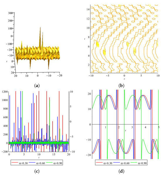
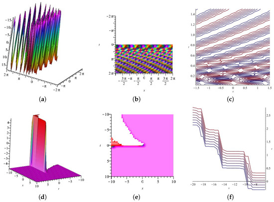
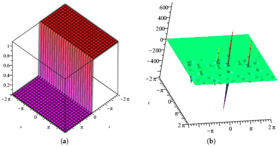
The plots of $u_1,\cdots ,u_4$ are displayed in Figure 1, Figure 2, Figure 3, Figure 4 and Figure 5, for two different cases $\lambda \eta >0$ and $\lambda \eta <0,$ for specific values $\eta =3,\lambda =2,\alpha =\frac{2}{5},D=2,C=3,$ and $\eta =3,\lambda =-2,\alpha =\frac{2}{5},$ $D=2,C=3,$ respectively.

Figure 1. The (a–d) display the 3D, 2D and the contour plots of $u_{1,2},$ for $\lambda \eta >0.$

Figure 2. The (a–d) display the 3D, 2D and the contour plots of $u_{1,2},$ for $\eta \lambda <0.$

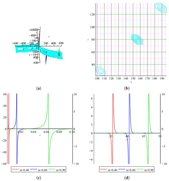
Figure 3. The (a,b) display the 3D plots of $u_{3,4}$, for $\lambda \eta >0$ and $\lambda \eta <0$.

Figure 4. The (a,b) display the 3D plots of $u_{5,6}$, for $\lambda \eta <0$ and $\lambda \eta >0.$

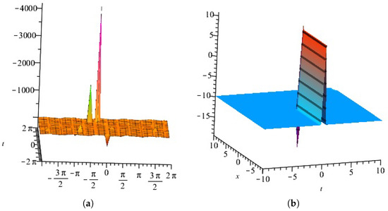
Figure 5. The (a–f) display the 3D, 2D and the contour plots of $u_{7,8}$, for $\lambda \eta >0$ and $\lambda \eta <0$.

Example 2.

Here, we consider the SRLW Equation (3), where $D^{\gamma }$ is the conformable derivative of order $\gamma ,$ given by

$$D_{\xi }^{\gamma }\left(\varpi \right)=\underset{ϵ⟶0}{lim}{\displaystyle \frac{\varpi (\xi +ϵ{\xi }^{1-\gamma })-\varpi \left(\xi \right)}{ϵ}},\xi >0,0<\gamma ⩽1,$$

in which $\varpi :[0,\infty )⟶\mathbb{R}$ is a given function.

If the above limit exists, then ϖ is called γ-differentiable. Assume $0<\gamma ⩽1,$ and ϖ and ${\varpi }^{\prime }$ be γ-differentiable at point $\xi >0,$ then $D^{\gamma }$ has the following properties:

∘

$D^{\gamma }(c\varpi +d{\varpi }^{\prime })=c{D}^{\gamma }\left(\varpi \right)+d{D}^{\gamma }\left({\varpi }^{\prime }\right)$ where $c,d\in \mathbb{R},$

∘

$D^{\gamma }\left({\xi }^n\right)=n{\xi }^{n-\gamma }$, where $n\in \mathbb{R},$

∘

$D^{\gamma }\left(\chi \right)=0⟹\varpi \left(\xi \right)=\chi \left(\mathit{is}\mathit{a}\mathit{constant}\right),$

∘

$D^{\gamma }\left(\varpi {\varpi }^{\prime }\right)=\varpi D^{\gamma }\left({\varpi }^{\prime }\right)+{\varpi }^{\prime }{D}^{\gamma }\left(\varpi \right),$

∘

$D^{\gamma }\left(\varpi \right)\left(\xi \right)={\xi }^{1-\gamma }{\displaystyle \frac{d\varpi }{d\xi }}\left(\xi \right),$

∘

$D^{\gamma }\left({\displaystyle \frac{\varpi }{{\varpi }^{\prime }}}\right)={\displaystyle \frac{{\varpi }^{\prime }{D}^{\gamma }\left(\varpi \right)-\varpi D^{\gamma }\left({\varpi }^{\prime }\right)}{{\left({\varpi }^{\prime }\right)}^2}}.$

Now, using the following transformation

$$\epsilon ={\displaystyle \frac{\alpha x^{\gamma }}{\Gamma (1+\gamma )}}+{\displaystyle \frac{\beta t^{\gamma }}{\Gamma (1+\gamma )}},u(x,t)=u\left(\epsilon \right),$$

(59)

Equation (3) turns into

$$\begin{array}{c}\hfill {\beta }^2{u}^{″}+{\alpha }^2{u}^{″}+\beta \alpha u{u}^{″}+\beta \alpha {\left(u^{\prime }\right)}^2+{\beta }^2{\alpha }^2{u}^{\left(\mathit{iv}\right)}=0.\end{array}$$

(60)

Integrating (60) twice yields

$${\beta }^2{\alpha }^2{u}^{″}+({\beta }^2+{\alpha }^2+k)u+{\displaystyle \frac{1}{2}}\beta \alpha u^2+\vartheta =0,$$

where k and ϑ are integral constants. For simplicity, we set $\vartheta =0.$ therefore, we get

$$\begin{array}{c}\hfill {\beta }^2{\alpha }^2{u}^{″}+({\beta }^2+{\alpha }^2+k)u+{\displaystyle \frac{1}{2}}\beta \alpha u^2=0.\end{array}$$

(61)

Here, we get the balancing number $2N=N+2$ or $N=2.$

Suppose the solution of (61) can be given by

$$u\left(\epsilon \right)=a_0+a_1\left({\displaystyle \frac{G^{\prime }}{G^2}}\right)+b_1{\left({\displaystyle \frac{G^{\prime }}{G^2}}\right)}^{-1}+a_2{\left({\displaystyle \frac{G^{\prime }}{G^2}}\right)}^2+b_2{\left({\displaystyle \frac{G^{\prime }}{G^2}}\right)}^{-2},$$

(62)

in which $a_0,b_1,a_1,b_2,a_2$ are constant to be determined later.

Inserting Equation (62) with Equation (10) into Equation (61) and collecting all terms with the same power of $\frac{G^{\prime }}{G^2},$ and then equating each coefficients of this polynomial to zero, we get the following system of algebraic equations:

$$\begin{array}{ccc}& & {\left({\displaystyle \frac{G^{\prime }}{G^2}}\right)}^{-4}:\frac{1}{2}\beta \alpha b_2^2+6{\beta }^2{\alpha }^2{b}_2{\eta }^2=0,\hfill \\ & & {\left({\displaystyle \frac{G^{\prime }}{G^2}}\right)}^{-3}:2{\alpha }^2{\beta }^2{\eta }^2{b}_1+\alpha \beta b_1{b}_2=0,\hfill \\ & & {\left({\displaystyle \frac{G^{\prime }}{G^2}}\right)}^{-2}:\frac{1}{2}\beta \alpha b_1^2+8{\beta }^2{\alpha }^2{b}_2\lambda \eta +\beta \alpha a_0{b}_2+b_{2}k+b_2{\alpha }^2+b_2{\beta }^2=0,\hfill \\ & & {\left({\displaystyle \frac{G^{\prime }}{G^2}}\right)}^{-1}:2{\alpha }^2{\beta }^2\eta \lambda b_1+\alpha \beta a_0{b}_1+\alpha \beta a_1{b}_2+{\alpha }^2{b}_1+{\beta }^2{b}_1+k{b}_1=0,\hfill \\ & & {\left({\displaystyle \frac{G^{\prime }}{G^2}}\right)}^0:\beta \alpha a_1{b}_1+\beta \alpha a_2{b}_2+2{\alpha }^2{\beta }^2{a}_2{\eta }^2+2{\beta }^2{\alpha }^2{b}_2{\lambda }^2+a_0{\alpha }^2+a_0{\beta }^2+a_{0}k+\frac{1}{2}\beta \alpha a_0^2,\hfill \\ & & {\left({\displaystyle \frac{G^{\prime }}{G^2}}\right)}^1:2{\alpha }^2{\beta }^2\eta \lambda a_1+\alpha \beta a_0{a}_1+\alpha \beta a_2{b}_1+{\alpha }^2{a}_1+{\beta }^2{a}_1+k{a}_1=0,\hfill \\ & & {\left({\displaystyle \frac{G^{\prime }}{G^2}}\right)}^2:\frac{1}{2}\beta \alpha a_1^2+8{\beta }^2{\alpha }^2{a}_2\lambda \eta +\beta \alpha a_0{a}_2+a_2{\alpha }^2+a_2{\beta }^2+a_{2}k=0,\hfill \\ & & {\left({\displaystyle \frac{G^{\prime }}{G^2}}\right)}^3:2{\alpha }^2{\beta }^2{\lambda }^2{a}_1+\alpha \beta a_1{a}_2=0,\hfill \\ & & {\left({\displaystyle \frac{G^{\prime }}{G^2}}\right)}^4:\frac{1}{2}\beta \alpha a_2^2+6{\beta }^2{\alpha }^2{a}_2{\lambda }^2=0.\hfill \end{array}$$

Solving the above system of nonlinear algebraic equation, we get

$$\begin{array}{ccc}& & \eta =\eta ,k=-\frac{1}{2}{a}_0\alpha \beta -{\alpha }^2-{\beta }^2,\lambda =\lambda ,a_0=a_0,a_1=0,a_2=0,b_1=0,b_2=0,\hfill \end{array}$$

(63)

$$\begin{array}{ccc}& & \eta =\eta ,k=k,\lambda =\lambda ,a_0=0,a_1=0,a_2=0,b_1=0,b_2=0,\hfill \end{array}$$

(64)

$$\begin{array}{ccc}& & \eta =\eta ,k=16{\alpha }^2{\beta }^2\eta \lambda -{\alpha }^2-{\beta }^2,\lambda =\lambda ,a_0=-24\lambda \eta \alpha \beta ,a_1=0,\hfill \\ & & a_2=-12{\lambda }^2\alpha \beta ,b_1=0,b_2=-12{\eta }^2\alpha \beta ,\hfill \end{array}$$

(65)

$$\begin{array}{ccc}& & \eta =\eta ,k=-16{\alpha }^2{\beta }^2\eta \lambda -{\alpha }^2-{\beta }^2,\lambda =\lambda ,a_0=8\lambda \eta \alpha \beta ,a_1=0,\hfill \\ & & a_2=-12{\lambda }^2\alpha \beta ,b_1=0,b_2=-12{\eta }^2\alpha \beta ,\hfill \end{array}$$

(66)

$$\begin{array}{ccc}& & \eta =\eta ,k=4\lambda \eta {\alpha }^2{\beta }^2-{\alpha }^2-{\beta }^2,\lambda =\lambda ,a_0=-12\lambda \eta \alpha \beta ,a_1=0,\hfill \\ & & a_2=0,b_1=0,b_2=-12{\eta }^2\alpha \beta ,\hfill \end{array}$$

(67)

$$\begin{array}{ccc}& & \eta =\eta ,k=-4\lambda \eta {\alpha }^2{\beta }^2-{\alpha }^2-{\beta }^2,\lambda =\lambda ,a_0=-4\lambda \eta \alpha \beta ,a_1=0,\hfill \\ & & a_2=0,b_1=0,b_2=-12{\eta }^2\alpha \beta ,\hfill \end{array}$$

(68)

$$\begin{array}{ccc}& & \eta =\eta ,k=4\lambda \eta {\alpha }^2{\beta }^2-{\alpha }^2-{\beta }^2,\lambda =\lambda ,a_0=-12\lambda \eta \alpha \beta ,a_1=0,\hfill \\ & & a_2=-12{\lambda }^2\alpha \beta ,b_1=0,b_2=0,\hfill \end{array}$$

(69)

$$\begin{array}{ccc}& & \eta =\eta ,k=-4\lambda \eta {\alpha }^2{\beta }^2-{\alpha }^2-{\beta }^2,\lambda =\lambda ,a_0=-4\lambda \eta \alpha \beta ,a_1=0,\hfill \\ & & a_2=-12{\lambda }^2\alpha \beta ,b_1=0,b_2=0.\hfill \end{array}$$

(70)

Inserting (65) in (62), we get

$$u\left(\epsilon \right)=-24\lambda \eta \alpha \beta -12{\lambda }^2\alpha \beta {\left({\displaystyle \frac{G^{\prime }}{G^2}}\right)}^2-12{\eta }^2\alpha \beta {\left({\displaystyle \frac{G^{\prime }}{G^2}}\right)}^{-2},$$

(71)

Therefore, we get three types of travelling wave solutions as follows:

• if $\lambda \eta >0;$

  $$u_1=-24\lambda \eta \alpha \beta -12{\lambda }^2\alpha \beta {\left({\xi }_1\right)}^2-12{\eta }^2\alpha \beta {\left({\xi }_1\right)}^{-2},$$

  (72)
  where

  $${\xi }_1=\sqrt{{\displaystyle \frac{\eta }{\lambda }}}\left({\displaystyle \frac{Ccos\left(\sqrt{\eta \lambda }({\displaystyle \frac{\alpha x^{\gamma }}{\Gamma (1+\gamma )}}+{\displaystyle \frac{\beta t^{\gamma }}{\Gamma (1+\gamma )}})\right)+Dsin\left(\sqrt{\eta \lambda }({\displaystyle \frac{\alpha x^{\gamma }}{\Gamma (1+\gamma )}}+{\displaystyle \frac{\beta t^{\gamma }}{\Gamma (1+\gamma )}})\right)}{Dcos\left(\sqrt{\eta \lambda }\epsilon \right)-Csin\left(\sqrt{\eta \lambda }({\displaystyle \frac{\alpha x^{\gamma }}{\Gamma (1+\gamma )}}+{\displaystyle \frac{\beta t^{\gamma }}{\Gamma (1+\gamma )}})\right)}}\right),$$
• if $\lambda \eta <0;$

  $$u_2=-24\lambda \eta \alpha \beta -12{\lambda }^2\alpha \beta {\left({\xi }_2\right)}^2-12{\eta }^2\alpha \beta {\left({\xi }_2\right)}^{-2},$$

  (73)
  where

  $${\xi }_2=-{\displaystyle \frac{\sqrt{\left|\eta \lambda \right|}}{\lambda }}\left({\displaystyle \frac{Csinh\left(2\sqrt{\left|\eta \lambda \right|}({\displaystyle \frac{\alpha x^{\gamma }}{\Gamma (1+\gamma )}}+{\displaystyle \frac{\beta t^{\gamma }}{\Gamma (1+\gamma )}})\right)+Ccosh\left(2\sqrt{\left|\eta \lambda \right|}({\displaystyle \frac{\alpha x^{\gamma }}{\Gamma (1+\gamma )}}+{\displaystyle \frac{\beta t^{\gamma }}{\Gamma (1+\gamma )}})\right)+D}{Csinh\left(2\sqrt{\left|\eta \lambda \right|}({\displaystyle \frac{\alpha x^{\gamma }}{\Gamma (1+\gamma )}}+{\displaystyle \frac{\beta t^{\gamma }}{\Gamma (1+\gamma )}})\right)+Ccosh\left(2\sqrt{\left|\eta \lambda \right|}({\displaystyle \frac{\alpha x^{\gamma }}{\Gamma (1+\gamma )}}+{\displaystyle \frac{\beta t^{\gamma }}{\Gamma (1+\gamma )}})\right)-D}}\right),$$
• if $\lambda \ne 0,\eta =0;$

  $$u_3=-24\lambda \eta \alpha \beta -12{\lambda }^2\alpha \beta {\left({\xi }_3\right)}^2-12{\eta }^2\alpha \beta {\left({\xi }_3\right)}^{-2},$$

  (74)
  where

  $${\xi }_3=-{\displaystyle \frac{C}{\lambda (C({\displaystyle \frac{\alpha x^{\gamma }}{\Gamma (1+\gamma )}}+{\displaystyle \frac{\beta t^{\gamma }}{\Gamma (1+\gamma )}})+D)}},$$
  where $C,D\ne 0.$

The plots of (72) and (73) are displayed in Figure 6 and Figure 7, for $\eta =2,\lambda =3,\alpha =\frac{1}{2},\beta =\frac{1}{3},$$\gamma =\frac{1}{2},D=2,C=3,$ and $\eta =-2,\lambda =3,\alpha =\frac{1}{2},\beta =\frac{1}{3},\gamma =\frac{1}{2},D=2,C=3,$ respectively.

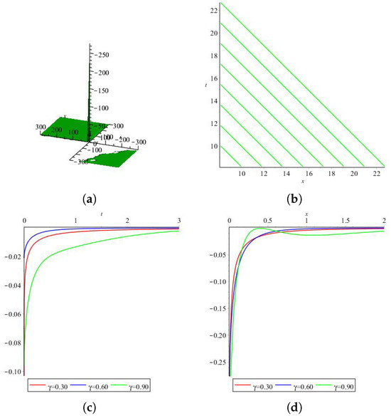
Figure 6. The (a–d) display the 3D, 2D and the contour plots of (72).

Figure 7. The (a–d) display the 3D, 2D and the contour plots of (73).

4. Application of the $\frac{{\mathit{G}}^{\prime }}{\mathit{G}}$-Expansion Method

Example 3.

Assume the nonlinear time fractional Harry Dym Equation (1).

Now, we employ the transformations (27), which represents a new dependent variable.

In a similar way presented in Example 1 in Section 3, we consider the ODE (33). Here, we get the balancing number $3N=N+2$ or $N=1.$

Suppose that the solution of (33) can be given by

$$\psi \left(\epsilon \right)=a_0+a_1\left({\displaystyle \frac{G^{\prime }}{G}}\right),$$

(75)

in which $a_0,a_1$ are constants to be determined later.

Inserting Equation (75) with Equation (17) into Equation (33) and collecting all terms with the same power of ${\displaystyle \frac{G^{\prime }}{G}},$ and then equating each coefficient of this polynomial to zero, we get the following system of algebraic equations:

$$\begin{array}{ccc}& & {\left({\displaystyle \frac{G^{\prime }}{G}}\right)}^3:-{\displaystyle \frac{a_1^3}{2}}+2a_1=0,\hfill \\ & & {\left({\displaystyle \frac{G^{\prime }}{G}}\right)}^2:-{\displaystyle \frac{3}{2}}{a}_0{a}_1^2+3a_1\lambda =0,\hfill \\ & & {\left({\displaystyle \frac{G^{\prime }}{G}}\right)}^1:-c{a}_1-\frac{3}{2}{a}_0^2{a}_1+a_1{\lambda }^2+2a_1\eta =0,\hfill \\ & & {\left({\displaystyle \frac{G^{\prime }}{G}}\right)}^0:-c{a}_0+a_1\eta \lambda -{\displaystyle \frac{a_0^3}{2}}=0.\hfill \end{array}$$

Solving the above system of nonlinear algebraic equation, we get

$$a_0=\mp \lambda ,a_1=\mp 2,c=-0.5({\lambda }^2-4\eta ).$$

(76)

Inserting (76) in (75), we get

$$\psi \left(\epsilon \right)=\pm 2\left({\displaystyle \frac{G^{\prime }}{G}}\right)\pm \lambda .$$

(77)

Therefore, we get three types of travelling wave solutions as follows:

Case 1: ${\lambda }^2-4\eta >0;$

$$\begin{array}{ccc}\hfill & & u_{1,2}(x,t)=\pm \sqrt{2(-0.5({\lambda }^2-4\eta ))}.\hfill \\ & & \left({\displaystyle \frac{iCcos\left(\sqrt{\frac{(-0.5({\lambda }^2-4\eta ))}{2}}(x-\frac{(-0.5({\lambda }^2-4\eta ))t^{\alpha }}{\Gamma (1+\alpha )})\right)+Dsin\left(\sqrt{\frac{(-0.5({\lambda }^2-4\eta ))}{2}}(x-\frac{(-0.5({\lambda }^2-4\eta ))t^{\alpha }}{\Gamma (1+\alpha )})\right)}{-iCsin\left(\sqrt{\frac{(-0.5({\lambda }^2-4\eta ))}{2}}(x-\frac{(-0.5({\lambda }^2-4\eta ))t^{\alpha }}{\Gamma (1+\alpha )})\right)+Dcos\left(\sqrt{\frac{(-0.5({\lambda }^2-4\eta ))}{2}}(x-\frac{(-0.5({\lambda }^2-4\eta ))t^{\alpha }}{\Gamma (1+\alpha )})\right)}}\right),\hfill \end{array}$$

Case 2: ${\lambda }^2-4\eta <0;$

$$\begin{array}{ccc}\hfill & & u_{1,2}(x,t)=\pm i\sqrt{2(-0.5({\lambda }^2-4\eta ))}.\hfill \\ & & \left({\displaystyle \frac{-Csin\left(\sqrt{\frac{(-0.5({\lambda }^2-4\eta ))}{2}}(x-\frac{(-0.5({\lambda }^2-4\eta ))t^{\alpha }}{\Gamma (1+\alpha )})\right)+Dcos\left(\sqrt{\frac{(-0.5({\lambda }^2-4\eta ))}{2}}(x-\frac{(-0.5({\lambda }^2-4\eta ))t^{\alpha }}{\Gamma (1+\alpha )})\right)}{Ccos\left(\sqrt{\frac{(-0.5({\lambda }^2-4\eta ))}{2}}(x-\frac{(-0.5({\lambda }^2-4\eta ))t^{\alpha }}{\Gamma (1+\alpha )})\right)+Dsin\left(\sqrt{\frac{(-0.5({\lambda }^2-4\eta ))}{2}}(x-\frac{(-0.5({\lambda }^2-4\eta ))t^{\alpha }}{\Gamma (1+\alpha )})\right)}}\right),\hfill \end{array}$$

Case 3: ${\lambda }^2-4\eta =0;$

$$u_{1,2}(x,t)=\pm {\displaystyle \frac{D}{D(x-\frac{(-0.5({\lambda }^2-4\eta ))t^{\alpha }}{\Gamma (1+\alpha )})+C}},$$

(78)

where $C,D\ne 0.$

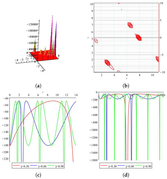
The plots of $u_1,\cdots ,u_4$ are displayed in Figure 8 and Figure 9, for two different cases ${\lambda }^2-4\eta >0$ and ${\lambda }^2-4\eta <0,$ for specific values $\eta =-3, \lambda =2, \alpha =\frac{2}{5}, D=2, C=3,$ and $\eta =3, \lambda =2,$$\alpha =\frac{2}{5}, D=2, C=3,$ respectively.

Figure 8. The (a,b) display the 3D and the contour plots of $u_{1,2}$, for ${\lambda }^2-4\eta >0$.

Figure 9. The (a,b) display the plots of real and imaginery part of $u_{1,2}$, for ${\lambda }^2-4\eta <0$.

5. Comparing the $\frac{{\mathit{G}}^{\prime }}{\mathit{G}}$-Expansion and the $\frac{{\mathit{G}}^{\prime }}{{\mathit{G}}^{\mathbf{2}}}$-Expansion Methods

Here, diverse values of the solutions of (1) obtained through the $\frac{G^{\prime }}{G^2}$-expansion method and the $\frac{G^{\prime }}{G}$-expansion method are presented in Table 1 and Table 2.

Table 1. Diverse values of the solutions of (1) obtained through the $\frac{G^{\prime }}{G^2}$-expansion method.

	$\mathit{\lambda }\mathit{\eta }>0$				$\mathit{\lambda }\mathit{\eta }<0$
$\mathit{x}=\mathit{t}$	${\mathit{u}}_{\mathbf{1},\mathbf{2}}(\mathit{x},\mathit{t})$	${\mathit{u}}_{\mathbf{3},\mathbf{4}}(\mathit{x},\mathit{t})$	${\mathit{u}}_{\mathbf{5},\mathbf{6}}(\mathit{x},\mathit{t})$	${\mathit{u}}_{\mathbf{7},\mathbf{8}}(\mathit{x},\mathit{t})$	${\mathit{u}}_{\mathbf{1},\mathbf{2}}(\mathit{x},\mathit{t})$	${\mathit{u}}_{\mathbf{3},\mathbf{4}}(\mathit{x},\mathit{t})$	${\mathit{u}}_{\mathbf{5},\mathbf{6}}(\mathit{x},\mathit{t})$	${\mathit{u}}_{\mathbf{7},\mathbf{8}}(\mathit{x},\mathit{t})$
0.001	±10.8391	±5.1739	±3.0254	±7.9327	±0.0069	±9.7979	±4.9993	±4.8005
0.010	±11.4354	±3.9987	±3.0052	±7.9859	0.0000	±9.7979	±4.8991	±4.8988
0.100	±15.5875	±0.9025	±1.6523	±14.5247	0.0000	±9.7979	±4.8989	±4.8989
1.001	±16.1931	±15.2886	±9.8816	±2.4287	0.0000	±9.7979	±4.8989	±4.8989
1.010	±13.5703	±10.6300	±33.0590	±0.7259	0.0000	±9.7979	±4.8989	±4.8989
1.100	±18.5057	±4.9848	±1.4733	±13.7668	0.0000	±9.7979	±4.8989	±4.8989

Table 2. Diverse values of the solutions of (1) obtained through $\frac{G^{\prime }}{G}$-expansion method.

	${\mathit{\lambda }}^2-4\mathit{\eta }>0$	${\mathit{\lambda }}^2-4\mathit{\eta }<0$
$\mathit{x}=\mathit{t}$	${\mathit{u}}_{\mathbf{1},\mathbf{2}}(\mathit{x},\mathit{t})$	${\mathit{u}}_{\mathbf{1},\mathbf{2}}(\mathit{x},\mathit{t})$
0.001	$\pm 4.1671$	0.0000
0.010	±4.0050	0.0000
0.100	±4.0000	0.0000
1.001	±4.0000	0.0000
1.010	±4.0000	0.0000
1.100	±4.0000	0.0000

As you can see, the obtained solutions through the $\frac{G^{\prime }}{G^2}$-expansion method present a better description of Equation (1) than the obtained solutions through the $\frac{G^{\prime }}{G}$-expansion method.

The $\frac{G^{\prime }}{G^2}$-expansion method and the $\frac{G^{\prime }}{G}$-expansion method are related to traveling wave solutions of NPDEs only. As mentioned before, there exist MWSs to NPDEs. We are interested in a novel approach for obtaining MWSs to NPDEs, and the MEFM formulates a solution algorithm for calculating MWSs to NPDEs. In Section 6, we present two different examples of the MEFM.

6. Application of the Multi-Exp-Function-Method

6.1. Example 1

Here, we apply the MEFM to obtain the novel analytical solutions for (4).

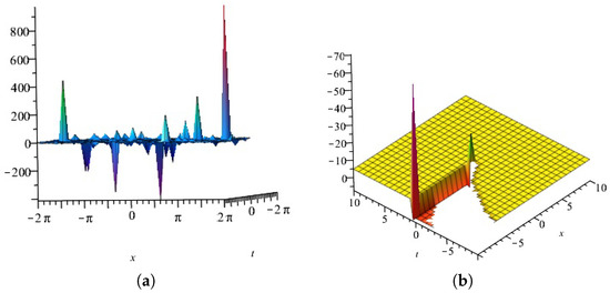
• One wave solutions for (4):
  First, consider ${\epsilon }_1={\epsilon }_1(x,y,t)$ as

  $${\epsilon }_1={\varpi }_{1}exp(S_{1}x+R_{1}y-{\omega }_{1}t),$$

  (79)

  where ${\varpi }_1,S_1,R_1$, and ${\omega }_1$ are constants. Now, ${\epsilon }_1$ has the following relations

  $${\epsilon }_{1,x}=S_1{\epsilon }_1,{\epsilon }_{1,y}=R_1{\epsilon }_1,{\epsilon }_{1,t}=-{\omega }_1{\epsilon }_1.$$

  (80)
  Therefore, we assume

  $$\begin{array}{ccc}& & \mathcal{K}\left({\epsilon }_1\right)=P_0+P_1{\epsilon }_1,\hfill \end{array}$$

  (81)

  $$\begin{array}{ccc}& & \mathcal{H}\left({\epsilon }_1\right)=Q_0+Q_1{\epsilon }_1,\hfill \end{array}$$

  (82)

  where $P_0,P_1,Q_0,$ and $Q_1$ are fixed to be determined from (4). Thus, we get

  $$u(x,t)={\displaystyle \frac{\mathcal{K}\left({\epsilon }_1\right)}{\mathcal{H}\left({\epsilon }_1\right)}}={\displaystyle \frac{P_0+P_1{\epsilon }_1}{Q_0+Q_1{\epsilon }_1}}.$$

  (83)
  By setting (83) into (4), we get:

  $$\begin{array}{c}{P}_1=\mathrm{arbitrary},\hfill \\ {\omega }_1:{\displaystyle \frac{1}{2}}{\displaystyle \frac{5i\sqrt{3}{R}_1^2+10S_1^2+2S_1{R}_1-5R_1^2}{R_1}}.\hfill \end{array}$$

  (84)
  By inserting (84) in (83), the one wave solutions can be presented by $u_1$.
  The real part of $u_1$ is displayed in Figure 10 for $S_1=7, R_1=-5, Q_1=-0.70$, $Q_0=0.40, P_0=0.90, P_1=3,$ (a) is three dimensional with $y=2.$ Here, (b), (c), and (d) exploit the $z,y,x$–axis orientation, respectively. Additionally, (e) is the contour plot. In addition, the imaginary part of equation $u_1$ is displayed in Figure 11 for $S_1=7,R_1=-5$, $Q_1=-0.70,Q_0=0.40,P_0=0.90,P_1=3,$ (a) is three dimensional with $y=2.$ Here, (b), (c), and (d) exploit the $z,y,x$–axis, orientation, respectively. Additionally, (e) is the contour plot.
  

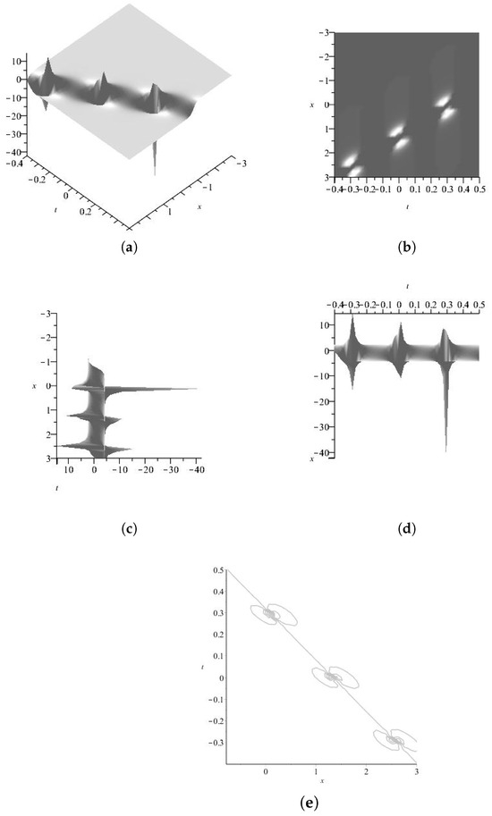  Figure 10. The (a–e) display the 2D, 3D and the contour plots of the real part of u₁.
  

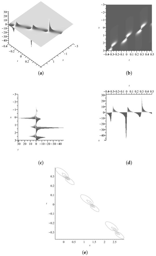  Figure 11. The (a–e) display the 2D, 3D and the contour plots of the imaginary part of $u_1.$
• Two wave solutions for (4):
  Consider ${\epsilon }_i={\epsilon }_i(x,y,t),i=1,2,$ such that

  $${\epsilon }_i={\varpi }_{i}exp(S_{i}x+R_{i}y-{\omega }_{i}t),i=1,2$$

  (85)

  in which $S_i,$ ${\varpi }_i,$$R_i,$ and ${\omega }_i$ are fixed. Now, we have

  $${\epsilon }_{i,y}=R_i,{\epsilon }_{i,x}=S_i{\epsilon }_i,{\epsilon }_{i,t}=-{\omega }_i{\epsilon }_i,i=1,2.$$

  (86)
  Then, we assume

  $$\begin{array}{ccc}& & \mathcal{K}({\epsilon }_1,{\epsilon }_2)=2(S_1{\epsilon }_1+S_2{\epsilon }_2+P_{12}(S_1+S_2){\epsilon }_1{\epsilon }_2),\hfill \end{array}$$

  (87)

  $$\begin{array}{ccc}& & \mathcal{H}({\epsilon }_1,{\epsilon }_2)=1+{\epsilon }_1+{\epsilon }_2+P_{12}{\epsilon }_1{\epsilon }_2,\hfill \end{array}$$

  (88)

  where $P_{12}$ is a constant to be determined from (4). Therefore, we have

  $$u(x,t)={\displaystyle \frac{2(S_1{\epsilon }_1+S_2{\epsilon }_2+P_{12}(S_1+S_2){\epsilon }_1{\epsilon }_2)}{1+{\epsilon }_1+{\epsilon }_2+P_{12}{\epsilon }_1{\epsilon }_2}}.$$

  (89)
  Using (89) into (4), we get:

  $$\begin{array}{ccc}& & P_{12}=1,\hfill \\ & & {\omega }_1={\displaystyle \frac{1}{2}}{\displaystyle \frac{5i\sqrt{3}{R}_1^2+10S_1^2+2S_1{R}_1-5R_1^2}{R_1}},\hfill \\ & & {\omega }_2={\displaystyle \frac{1}{2}}{\displaystyle \frac{5i\sqrt{3}{R}_2^2+10S_2^2+2S_2{R}_2-5R_2^2}{R_2}}.\hfill \end{array}$$
  Using (89), we can show that the two wave solutions can be presented by $u_2.$ The real part of $u_2$ is displayed in Figure 12 for $S_1=3,S_2=-5,R_1=2,R_2=-7,$ (a) is three dimensional with $y=2.$ Here, (b), (c), and (d) exploit the $z,y,x$–axis, respectively. Additionally, (e) is the contour plot. In addition, the imaginary part of equation $u_2$ is displayed in Figure 13 for $S_1=3,S_2=-5,R_1=2,R_2=-7,$ (a) is three dimensional with $y=2.$ Here, (b), (c), and (d) exploit the $z,x,y$–axis orientation, respectively. Additionally, (e) is the contour plot.
  

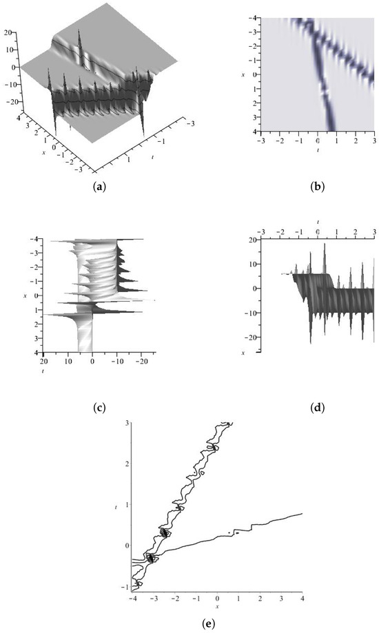  Figure 12. The (a–e) display the 2D, 3D and the contour plots of the real part of $u_2.$
  

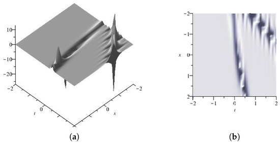
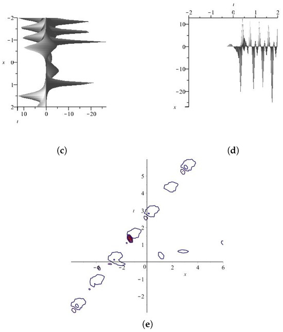  Figure 13. The (a–e) display the 2D, 3D and the contour plots of the imaginary part of u₂.
• Three wave solutions for (4):
  Consider ${\epsilon }_i={\epsilon }_i(x,y,t),i=1,2,3,$ such that

  $${\epsilon }_i={\varpi }_{i}exp(S_{i}x+R_{i}y-{\omega }_{i}t),i=1,2,3$$

  (90)

  where $S_i,$ ${\varpi }_i,$ and ${\omega }_i$ are fixed. Now, ${\epsilon }_i$ has the following relations

  $${\epsilon }_{i,x}=S_i{\epsilon }_i,{\epsilon }_{i,y}=R_i{\epsilon }_1,{\epsilon }_{i,t}=-{\omega }_i{\epsilon }_i,i=1,2,3.$$

  (91)
  Therefore, we assume

  $$\begin{array}{ccc}& & \mathcal{K}({\epsilon }_1,{\epsilon }_2,{\epsilon }_3)=2(S_1{\epsilon }_1+S_2{\epsilon }_2+S_3{\epsilon }_3+P_{12}(S_1+S_2){\epsilon }_1{\epsilon }_2\hfill \\ & & +P_{13}(S_1+S_3){\epsilon }_1{\epsilon }_3+P_{23}(S_2+S_3){\epsilon }_2{\epsilon }_3+P_{12}{P}_{13}{P}_{23}(S_1+S_2+S_3){\epsilon }_1{\epsilon }_2{\epsilon }_3),\hfill \end{array}$$

  and

  $$\begin{array}{ccc}& & \mathcal{H}({\epsilon }_1,{\epsilon }_2,{\epsilon }_3)=1+{\epsilon }_1+{\epsilon }_2+{\epsilon }_3+P_{12}{\epsilon }_1{\epsilon }_2+P_{13}{\epsilon }_1{\epsilon }_3+P_{23}{\epsilon }_2{\epsilon }_3\hfill \\ & & +P_{12}{P}_{13}{P}_{23}{\epsilon }_1{\epsilon }_2{\epsilon }_3,\hfill \end{array}$$

  where $P_{12},P_{13},$ and $P_{23}$ are fixed to be determined from (4). Thus, we get

  $$\begin{array}{c}u(x,t)=\left[2\right(S_1{\epsilon }_1+S_2{\epsilon }_2+S_3{\epsilon }_3+P_{12}(S_1+S_2){\epsilon }_1{\epsilon }_2\hfill \\ +P_{13}(S_1+S_3){\epsilon }_1{\epsilon }_3+P_{23}(S_2+S_3){\epsilon }_2{\epsilon }_3+P_{12}{P}_{13}{P}_{23}(S_1+S_2+S_3){\epsilon }_1{\epsilon }_2{\epsilon }_3\left)\right]/\hfill \\ \left[1+{\epsilon }_1+{\epsilon }_2+{\epsilon }_3+P_{12}{\epsilon }_1{\epsilon }_2+P_{13}{\epsilon }_1{\epsilon }_3+P_{23}{\epsilon }_2{\epsilon }_3+P_{12}{P}_{13}{P}_{23}{\epsilon }_1{\epsilon }_2{\epsilon }_3\right].\hfill \end{array}$$

  (92)
  Now, by setting (92) into (4) and solving the system of algebraic equations, we have:

  $$\begin{array}{c}{P}_{12}=1,\hfill \\ P_{13}=1,\hfill \\ P_{23}=1,\hfill \\ {\omega }_1={\displaystyle \frac{1}{2}}{\displaystyle \frac{5i\sqrt{3}{R}_1^2+10S_1^2+2S_1{R}_1-5R_1^2}{R_1}},\hfill \\ {\omega }_2={\displaystyle \frac{1}{2}}{\displaystyle \frac{5i\sqrt{3}{R}_2^2+10S_2^2+2S_2{R}_2-5R_2^2}{R_2}},\hfill \\ {\omega }_3={\displaystyle \frac{1}{2}}{\displaystyle \frac{5i\sqrt{3}{R}_3^2+10S_3^2+2S_3{R}_3-5R_3^2}{R_3}},\hfill \end{array}$$

  $$\begin{array}{c}{P}_{12}=1,\hfill \\ P_{13}=1,\hfill \\ P_{23}=1,\hfill \\ R_3={\displaystyle \frac{S_3{R}_2}{S_2}},\hfill \\ {\omega }_1={\displaystyle \frac{1}{2}}{\displaystyle \frac{5i\sqrt{3}{R}_1^2+10S_1^2+2S_1{R}_1-5R_1^2}{R_1}},\hfill \\ {\omega }_2={\displaystyle \frac{1}{2}}{\displaystyle \frac{5i\sqrt{3}{R}_2^2+10S_2^2+2S_2{R}_2-5R_2^2}{R_2}},\hfill \\ {\omega }_3={\displaystyle \frac{1}{2}}{\displaystyle \frac{S_3(5i\sqrt{3}{R}_2^2+10S_2^2+2S_2{R}_2-5R_2^2)}{R_2{S}_2}},\hfill \end{array}$$

  $$\begin{array}{c}{P}_{12}=1,\hfill \\ P_{13}=1,\hfill \\ P_{23}=1,\hfill \\ R_1={\displaystyle \frac{S_1{R}_3}{S_3}},\hfill \\ {\omega }_1={\displaystyle \frac{1}{2}}{\displaystyle \frac{S_1(5i\sqrt{3}{R}_3^2+10S_3^2+2S_3{R}_3-5R_3^2)}{R_3{S}_3}},\hfill \\ {\omega }_2={\displaystyle \frac{1}{2}}{\displaystyle \frac{5i\sqrt{3}{R}_2^2+10S_2^2+2S_2{R}_2-5R_2^2}{R_2}},\hfill \\ {\omega }_3={\displaystyle \frac{1}{2}}{\displaystyle \frac{5i\sqrt{3}{R}_3^2+10S_3^2+2S_3{R}_3-5R_3^2}{R_3}},\hfill \end{array}$$

  $$\begin{array}{c}{P}_{12}=1,\hfill \\ P_{13}=\mathrm{arbitrary},\hfill \\ P_{23}=\mathrm{arbitrary},\hfill \\ R_1={\displaystyle \frac{S_1{R}_2}{S_2}},\hfill \\ R_3={\displaystyle \frac{S_3{R}_2}{S_2}},\hfill \\ {\omega }_1={\displaystyle \frac{1}{2}}{\displaystyle \frac{S_1(5i\sqrt{3}{R}_2^2+10S_2^2+2S_2{R}_2-5R_2^2)}{R_2{S}_2}},\hfill \\ {\omega }_2={\displaystyle \frac{1}{2}}{\displaystyle \frac{5i\sqrt{3}{R}_2^2+10S_2^2+2S_2{R}_2-5R_2^2}{R_2}},\hfill \\ {\omega }_3={\displaystyle \frac{1}{2}}{\displaystyle \frac{S_3(5i\sqrt{3}{R}_2^2+10S_2^2+2S_2{R}_2-5R_2^2)}{R_2{S}_2}},\hfill \end{array}$$

  $$\begin{array}{c}{P}_{12}=\mathrm{arbitrary},\hfill \\ P_{13}=1,\hfill \\ P_{23}=1,\hfill \\ R_2={\displaystyle \frac{S_2{R}_1}{S_1}},\hfill \\ {\omega }_1={\displaystyle \frac{1}{2}}{\displaystyle \frac{5i\sqrt{3}{R}_1^2+10S_1^2+2S_1{R}_1-5R_1^2}{R_1}},\hfill \\ {\omega }_2={\displaystyle \frac{1}{2}}{\displaystyle \frac{S_2(5i\sqrt{3}{R}_1^2+10S_1^2+2S_1{R}_1-5R_1^2)}{R_1{S}_1}},\hfill \\ {\omega }_3={\displaystyle \frac{1}{2}}{\displaystyle \frac{5i\sqrt{3}{R}_3^2+10S_3^2+2S_3{R}_3-5R_3^2}{R_3}},\hfill \end{array}$$

  and

  $$\begin{array}{c}{P}_{12}=\mathrm{arbitrary},\hfill \\ P_{13}=\mathrm{arbitrary},\hfill \\ P_{23}=\mathrm{arbitrary},\hfill \\ R_2={\displaystyle \frac{S_2{R}_1}{S_1}},\hfill \\ R_3={\displaystyle \frac{S_3{R}_1}{S_1}},\hfill \\ {\omega }_1={\displaystyle \frac{1}{2}}{\displaystyle \frac{5i\sqrt{3}{R}_1^2+10S_1^2+2S_1{R}_1-5R_1^2}{R_1}},\hfill \\ {\omega }_2={\displaystyle \frac{1}{2}}{\displaystyle \frac{S_2(5i\sqrt{3}{R}_1^2+10S_1^2+2S_1{R}_1-5R_1^2)}{R_1{S}_1}},\hfill \\ {\omega }_3={\displaystyle \frac{1}{2}}{\displaystyle \frac{S_3(5i\sqrt{3}{R}_1^2+10S_1^2+2S_1{R}_1-5R_1^2)}{R_1{S}_1}}.\hfill \end{array}$$
  Thus, the three wave solutions can be presented by $u_{3,1},u_{3,2},u_{3,3},u_{3,4},u_{3,5}$, $u_{3,6},$ respectively.

The real part of $u_{3,1}$ is displayed in Figure 14 for $S_1=0.5,S_2=-0.7,k_3=1.20$, $R_1=-1.50,R_2=2,R_3=1.50,$ (a) is three dimensional with $y=2.$ Here, (b), (c), and (d) exploit the $z,y,x$–axis, orientation. Additionally, (e) is the contour plot.

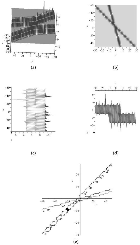
Figure 14. The (a–e) display the 2D, 3D and the contour plots of the real part of u_3,1.

The imaginary part of equation $u_{3,1}$ is displayed in Figure 15 for $S_1=0.5,$ $S_2=-0.7,k_3=1.20,R_1=-1.50$, $R_2=2,R_3=1.50,$ (a) is three dimensional with $y=2.$ Here, (b), (c), and (d) exploit the $z,y,x$–axis, orientation. Additionally, (e) is the contour plot.

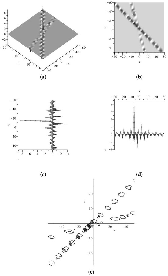
Figure 15. The (a–e) display the 2D, 3D and the contour plots of the imaginary part of $u_{3,1}.$

The real part of $u_{3,2}$ is displayed in Figure 16 for $S_1=3.50,S_2=-3.70,k_3=1.20$, $R_1=5,R_2=2.30,R_3=3,P_{23}=3,$ (a) is three dimensional with $y=2.$ Here, (b), (c), and (d) exploit the $z,x,y$–axis, orientation. Additionally, (e) is the contour plot.

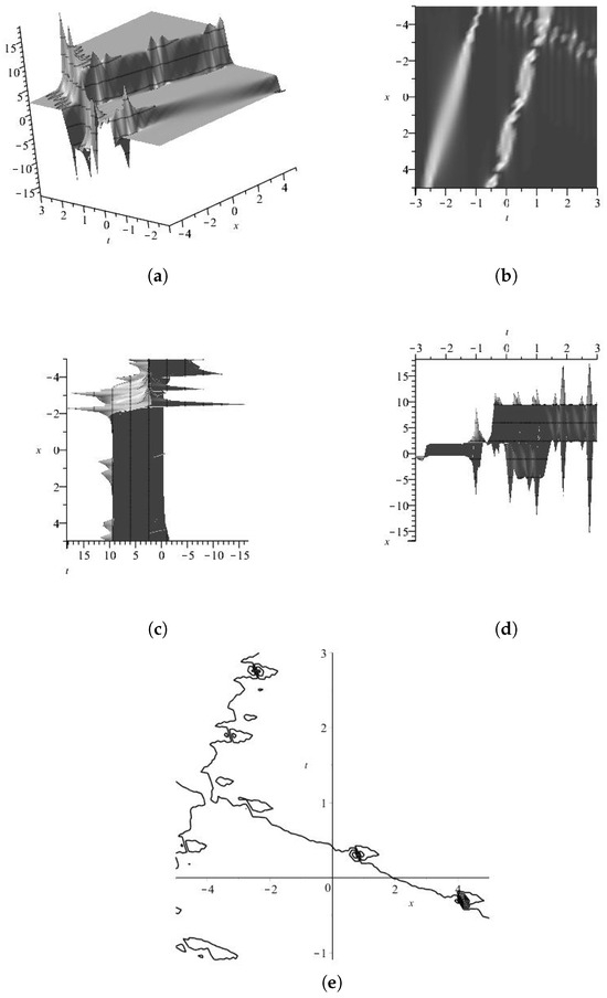
Figure 16. The (a–e) display the 2D, 3D and the contour plots of the real part of $u_{3,2}.$

The imaginary part of equation $u_{3,2}$ is displayed in Figure 17 for $S_1=3.50$, $S_2=-3.70$, $k_3=1.20$, $R_1=5,R_2=2.30,R_3=3,P_{23}=3,$ (a) is three dimensional with $y=2.$ Here, (b), (c), and (d) exploit the $z,y,x$–axis, orientation. Additionally, (e) is the contour plot.

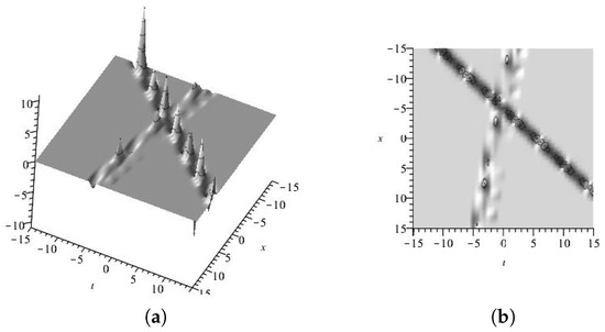
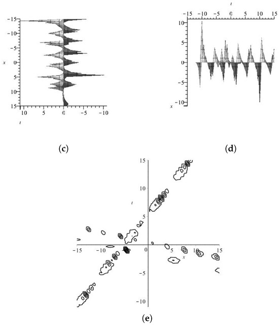
Figure 17. The (a–e) display the 2D, 3D and the contour plots of the imaginary part of u_3,2.

The real part of $u_{3,3}$ is displayed in Figure 18 for $S_1=3.50,S_2=-3.70,k_3=1.20$, $R_2=2.30,R_3=3,P_{13}=3,$ (a) is three dimensional with $y=2.$ Here, (b), (c), and (d) exploit the $z,y,x$–axis, orientation. Additionally, (e) is the contour plot.

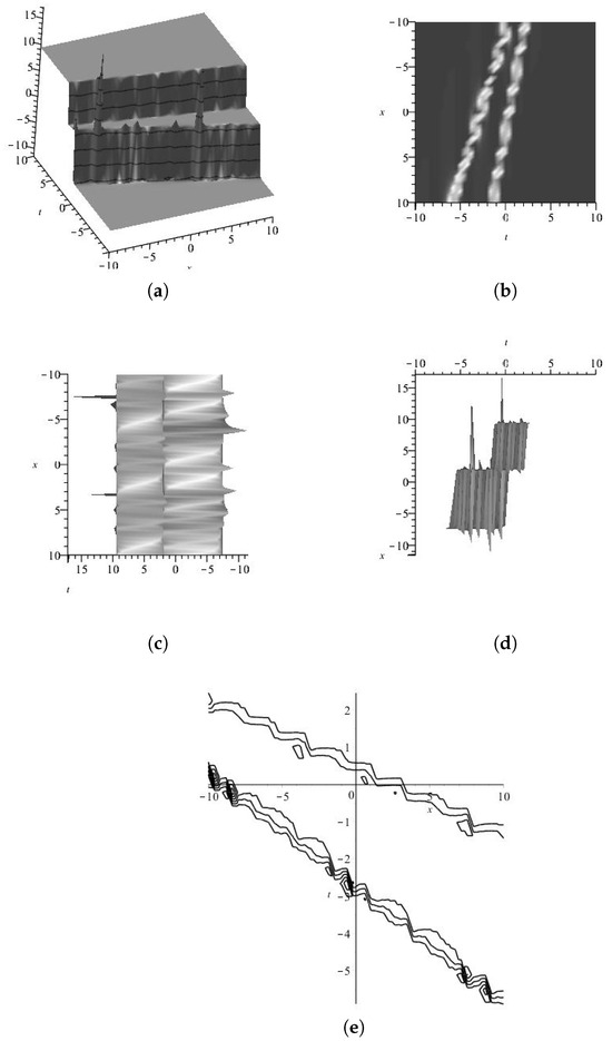
Figure 18. The (a–e) display the 2D, 3D and the contour plots of the real part of u_3,3.

The imaginary part of equation $u_{3,3}$ is displayed in Figure 19 for $S_1=3.50$, $S_2=-3.70$, $k_3=1.20,R_2=2.30,R_3=3$, $P_{13}=3,$ (a) is three dimensional with $y=2.$ Here, (b), (c), and (d) exploit the $z,y,x$-axis, orientation. Additionally, (e) is the contour plot.

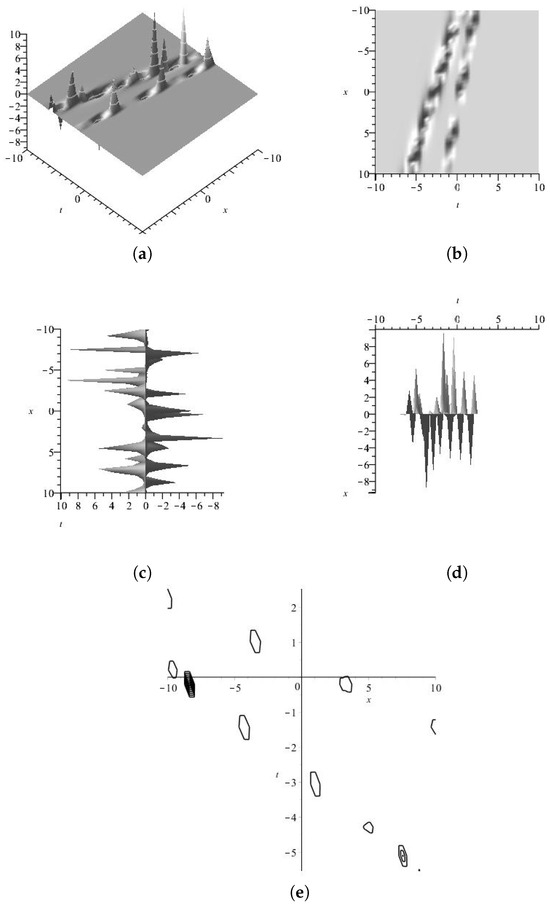
Figure 19. The (a–e) display the 2D, 3D and the contour plots of the imaginary part of $u_{3,3}.$

The real part of $u_{3,4}$ is displayed in Figure 20 for $S_1=3.50,S_2=-3.70,S_3=1.20$, $R_2=2.30,P_{23}=5,P_{13}=7,$ (a) is three dimensional with $y=2.$ Here, (b), (c), and (d) exploit the $z,y,x$–axis, orientation. Additionally, (e) is the contour plot.

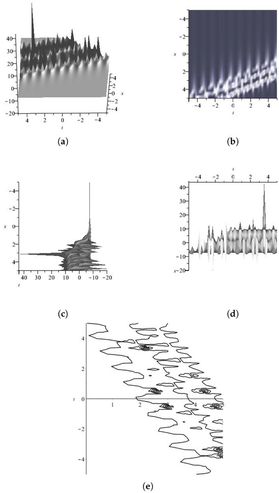
Figure 20. The (a–e) display the 2D, 3D and the contour plots of the real part of $u_{3,4}.$

The imaginary part of equation $u_{3,4}$ is displayed in Figure 21 for $S_1=3.50,$$S_2=-3.70$, $S_3=1.20,R_2=2.30,P_{23}=5$, $P_{13}=7,$ (a) is three dimensional with $y=2.$ Here, (b), (c), and (d) exploit the $z,y,x$–axis, orientation. Additionally, (e) is the contour plot.

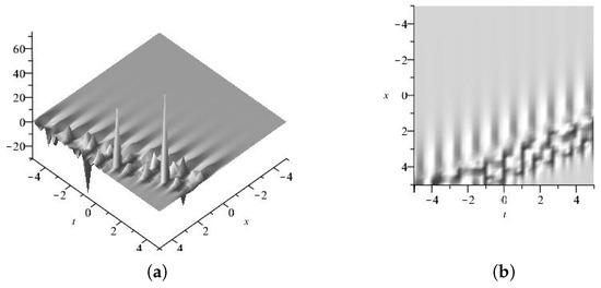
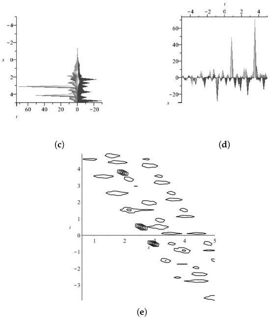
Figure 21. The (a–e) display the 2D, 3D and the contour plots of the imaginary part of u_3,4.

The real part of $u_{3,5}$ is displayed in Figure 22 for $S_1=3.50,$$S_2=-3.70$, $S_1=3.50$, $S_3=1.20,R_1=11,R_3=13,P_{23}=5,P_{12}=9,$ (a) is three dimensional with $y=2.$ Here, (b), (c), and (d) exploit the $z,y,x$–axis, orientation. Additionally, (e) is the contour plot.

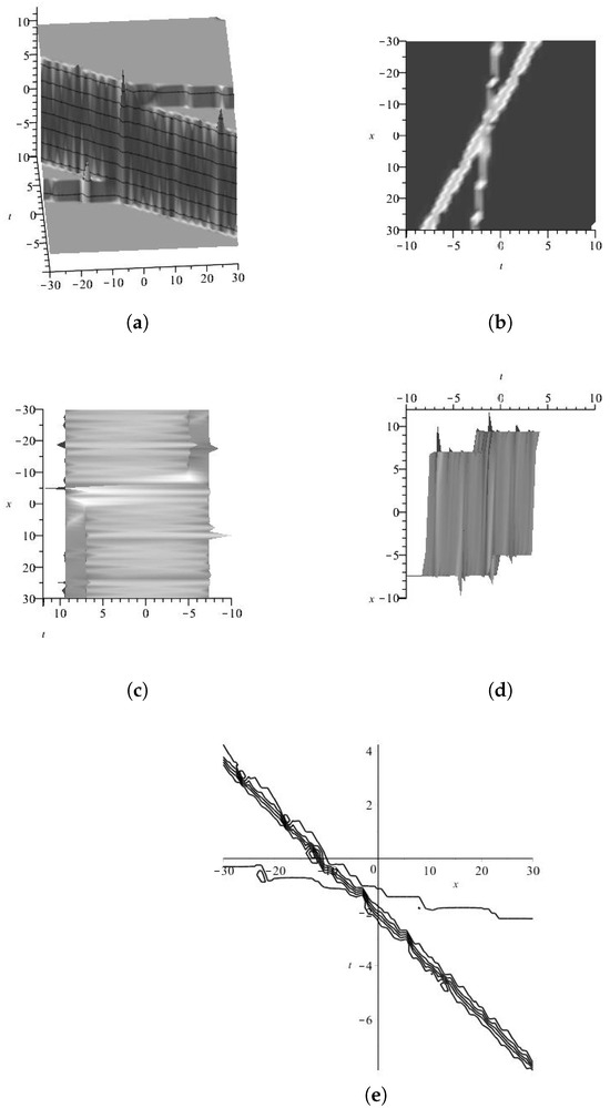
Figure 22. The (a–e) display the 2D, 3D and the contour plots of the real part of u_3,5.

The imaginary part of equation $u_{3,5}$ is displayed in Figure 23 for $S_1=3.50$, $S_2=-3.70$, $S_1=3.50,S_3=1.20,R_1=11,R_3=13,P_{23}=5,P_{12}=9,$ (a) is three dimensional with $y=2.$ Here, (b), (c), and (d) exploit the $z,y,x$–axis, orientation. Additionally, (e) is the contour plot.

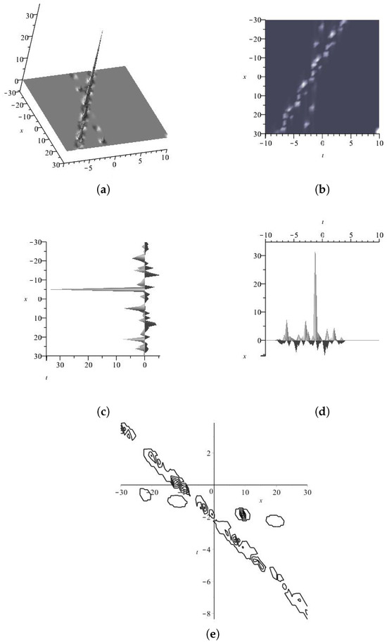
Figure 23. The (a–e) display the 2D, 3D and the contour plots of the imaginary part of $u_{3,5}.$

The real part of $u_{3,6}$ is displayed in Figure 24 for $S_1=3.50,S_2=-3.70,S_1=3.50$, $S_3=1.20,R_1=11,P_{23}=-11,P_{13}=13,P_{12}=9,$ (a) is three dimensional with $y=2.$ Here, (b), (c), and (d) exploit the $z,y,x$–axis, orientation. Additionally, (e) is the contour plot.

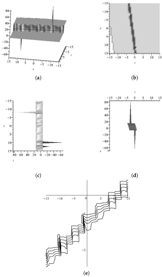
Figure 24. The (a–e) display the 2D, 3D and the contour plots of the real part of $u_{3,6}.$

The imaginary part of equation $u_{3,6}$ is displayed in Figure 25 for $S_1=3.50,S_2=-3.70$, $S_1=3.50,S_3=1.20,R_1=11,P_{23}=-11,P_{13}=13,P_{12}=9,$ (a) is three dimensional with $y=2.$ Here, (b), (c), and (d) exploit the $z,y,x$–axis orientation. Additionally, (e) is the contour plot.

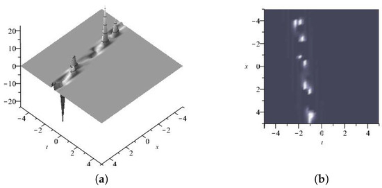
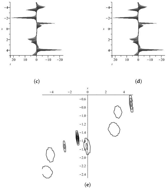
Figure 25. The (a–e) display the 2D, 3D and the contour plots of the imaginary part of u_3,6.

6.2. Example 2

In this subsection, we use the MEFM to get the novel analytical solutions for (5).

• One wave solutions for (5):
  In a similar way, we get

  $$\begin{array}{c}{P}_1=\mathrm{arbitrary},\hfill \\ {\omega }_1:-{\displaystyle \frac{5S_1^2-S_1{R}_1+5R_1^2}{R_1}}.\hfill \end{array}$$

  (93)
  By inserting (93) in (83), the one wave solutions can be presented by $v_1.$
  $v_1$ is displayed in Figure 26 for $S_1=7,R_1=-5,Q_1=-0.70,Q_0=0.40$, $P_0=0.90,P_1=3,$ (a) is three dimensional with $y=2.$ Here, (b), (c), and ( d) exploit the $z,y,x$–axis orientation. Additionally, (e) is the contour plot.
  

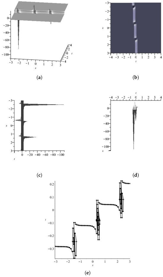  Figure 26. The (a–e) display the 2D, 3D and the contour plots of $v_1.$
• Two wave solutions for (5):
  In a similar way, we get

  $$\begin{array}{c}{P}_{12}=1,\hfill \\ {\omega }_1=-{\displaystyle \frac{5S_1^2-S_1{R}_1+5R_1^2}{R_1}},\hfill \\ {\omega }_2=-{\displaystyle \frac{5S_2^2-S_2{R}_2+5R_2^2}{R_2}}.\hfill \end{array}$$
  By setting the above values in (89), the two wave solutions can be presented by $v_2.$
  $v_2$ is displayed in Figure 27 for $S_1=3,S_2=-5,R_1=2,R_2=-7,$ (a) is three dimensional with $y=2.$ Here, (b), (c), and (d) exploit the z-axis, y-axis, x-axis orientation, respectively. Additionally, (e) is the contour plot.
  

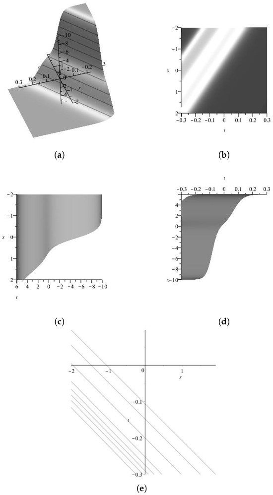  Figure 27. The (a–e) display the 2D, 3D and the contour plots of $v_2.$
• Three wave solutions for (5):
  In a similar way, we get

  $$\begin{array}{c}{P}_{12}=1,\hfill \\ P_{13}=1,\hfill \\ P_{23}=1,\hfill \\ {\omega }_1=-{\displaystyle \frac{5S_1^2-S_1{R}_1+5R_1^2}{R_1}},\hfill \\ {\omega }_2=-{\displaystyle \frac{5S_2^2-S_2{R}_1+5R_2^2}{R_2}},\hfill \\ {\omega }_3=-{\displaystyle \frac{5S_3^2-S_3{R}_3+5R_3^2}{R_3}},\hfill \end{array}$$

  $$\begin{array}{c}{P}_{12}=1,\hfill \\ P_{13}=\mathrm{arbitrary},\hfill \\ P_{23}=\mathrm{arbitrary},\hfill \\ R_1={\displaystyle \frac{S_1{R}_2}{S_2}},\hfill \\ R_3={\displaystyle \frac{S_3{R}_2}{S_3}},\hfill \\ {\omega }_1=-{\displaystyle \frac{S_1(5S_2^2-S_2{R}_2+5R_2^2)}{R_1{S}_2}},\hfill \\ {\omega }_2=-{\displaystyle \frac{5S_2^2-S_2{R}_2+5R_2^2}{R_2}},\hfill \\ {\omega }_3=-{\displaystyle \frac{S_3(5S_2^2-S_2{R}_2+5R_2^2)}{R_2{S}_2}},\hfill \end{array}$$

  $$\begin{array}{c}{P}_{12}=1,\hfill \\ P_{13}=\mathrm{arbitrary},\hfill \\ P_{23}=1,\hfill \\ R_1={\displaystyle \frac{S_1{R}_3}{S_3}},\hfill \\ R_3={\displaystyle \frac{S_3{R}_2}{S_3}},\hfill \\ {\omega }_1=-{\displaystyle \frac{S_1(5S_3^2-S_3{R}_3+5R_3^2)}{R_3{S}_3}},\hfill \\ {\omega }_2=-{\displaystyle \frac{5S_2^2-S_2{R}_2+5R_2^2}{R_2}},\hfill \\ {\omega }_3=-{\displaystyle \frac{5S_3^2-S_3{R}_3+5R_3^2}{R_3}},\hfill \end{array}$$

  and

  $$\begin{array}{c}{P}_{12}=\mathrm{arbitrary},\hfill \\ P_{13}=1,\hfill \\ P_{23}=1,\hfill \\ R_2={\displaystyle \frac{S_2{R}_1}{S_1}},\hfill \\ {\omega }_1=-{\displaystyle \frac{5S_1^2-S_1{R}_1+5R_1^2}{R_1}},\hfill \\ {\omega }_2=-{\displaystyle \frac{S_2(5S_1^2-S_1{R}_1+5R_1^2)}{R_1{S}_1}},\hfill \\ {\omega }_3=-{\displaystyle \frac{5S_3^2-S_3{R}_3+5R_3^2}{R_3}}.\hfill \end{array}$$
  Thus, the three wave solutions can be presented by $v_{3,1},v_{3,2},v_{3,3},v_{3,4},$ respectively.

$v_{3,1}$ is displayed in Figure 28 for $S_1=0.5,S_2=-0.7,S_3=1.20,R_1=-1.50$, $R_2=2,R_3=1.50,$ (a) is three dimensional with $y=2.$ Here, (b), (c), and (d) exploit the $z,y,x$–axis orientation. Additionally, (e) is the contour plot.

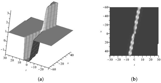
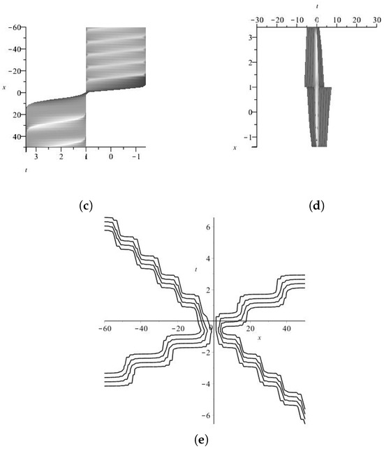
Figure 28. The (a–e) display the 2D, 3D and the contour plots of v_3,1.

$v_{3,2}$ is displayed in Figure 29 for $S_1=3.5,S_2=-3.7,S_3=1.20,R_2=2.30$, $P_{13}=\frac{3}{7},P_{23}=-\frac{5}{2},$ (a) is three dimensional with $y=2.$ Here, (b), (c), and (d) exploit the $z,y,x$–axis orientation. Additionally, (e) is the contour plot.

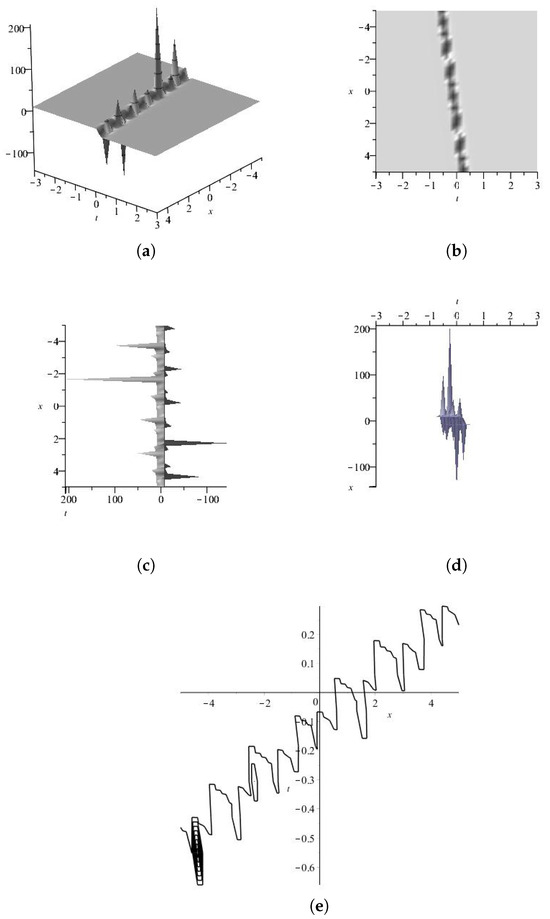
Figure 29. The (a–e) display the 2D, 3D and the contour plots of v_3,2.

$v_{3,3}$ is displayed in Figure 30 for $S_1=3.5,S_2=-3.7,S_3=1.20,R_2=2,R_3=3$, $P_{23}=\frac{5}{2},$ (a) is three dimensional with $y=2.$ Here, (b), (c), and (d) exploit the $z,y,x$–axis orientation. Additionally, (e) is the contour plot.

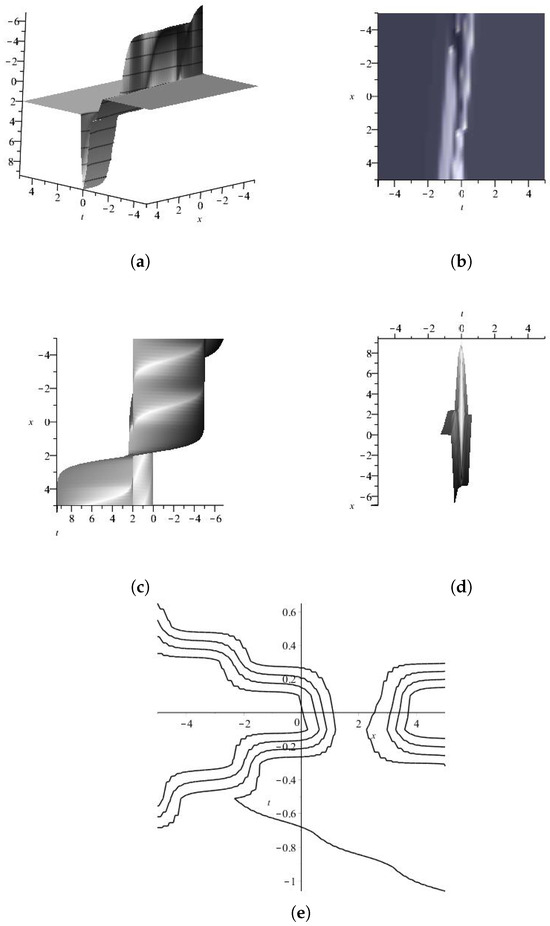
Figure 30. The (a–e) display the 2D, 3D and the contour plots of $v_{3,3}.$

$v_{3,4}$ is displayed in Figure 31 for $S_1=3.5,S_2=-3.7,S_3=4.20,R_1=-0.50$, $R_3=0.90,P_{12}=\frac{11}{5},$ (a) is three dimensional with $y=2.$ Here, (b), (c), and (d) exploit the $z,y,x$–axis orientation. Additionally, (e) is the contour plot.

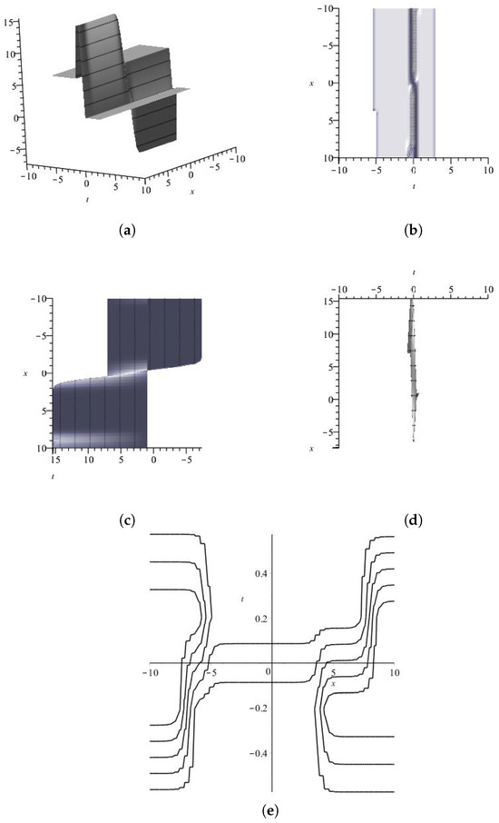
Figure 31. The (a–e) display the 2D, 3D and the contour plots of $v_{3,4}.$

Although the MEFM can obtain the MWSs to nonlinear equations, calculating each wave solution separately takes a lot of time and this can be one of the shortcomings of this method.

7. Concluding Remarks

In this paper, we applied three different methods, namely, the $\frac{G^{\prime }}{G}$-expansion method, the $\frac{G^{\prime }}{G^2}$-expansion method, and the MEFM to investigate the nonlinear time fractional Harry Dym equation in the Caputo sense and the symmetric regularized long wave equation in the conformable sense. In particular, we calculated the multiple wave solutions to (2 + 1)-dimensional equations by means of operating the MEFM, containing one, two, and triple-soliton-type solutions. It is obvious that this new technique has plenty of families of solutions, including rational exponential functions by choosing special parameters. Thus, the present paper provides encouragement for future research in soliton topics. The behaviors of the solutions for the known nonlinear equations gained via the MEFM by choosing the suitable values are cited in Figure 10 and Figure 31. Besides, numerical simulations involving the determination of the coefficients have been carried out to prove that the projected algorithm is efficient and applicable. An analytical study was performed for the solutions obtained using employing the aforementioned technique, revealing one, two, and triple-soliton-type solutions. The obtained results are beneficial for the study of wave propagation. The computations in the present paper were made with the aid of Maple.

References

- Aderyani, S.R.; Saadati, R.; Vahidi, J.; Allahviranloo, T. The exact solutions of the conformable time-fractional modified nonlinear Schrödinger equation by the Trial equation method and modified Trial equation method. Adv. Math. Phys. 2022, 2022, 4318192. [Google Scholar] [CrossRef]
- Aderyani, S.R.; Saadati, R.; Vahidi, J.; Gómez-Aguilar, J.F. The exact solutions of conformable time-fractional modified nonlinear Schrödinger equation by first integral method and functional variable method. Opt. Quantum Electron. 2022, 54, 218. [Google Scholar] [CrossRef]
- Aderyani, S.R.; Saadati, R.; O’Regan, D.; Alshammari, F.S. Describing Water Wave Propagation Using the G′G–Expansion Method. Mathematics 2022, 11, 191. [Google Scholar] [CrossRef]
- Tarla, S.; Ali, K.K.; Yilmazer, R.; Osman, M.S. New optical solitons based on the perturbed Chen-Lee-Liu model through Jacobi elliptic function method. Opt. Quantum Electron. 2022, 54, 131. [Google Scholar] [CrossRef]
- Yasmin, H.; Aljahdaly, N.H.; Saeed, A.M.; Shah, R. Probing families of optical soliton solutions in fractional perturbed Radhakrishnan–Kundu–Lakshmanan model with improved versions of extended direct algebraic method. Fractal Fract. 2023, 7, 512. [Google Scholar] [CrossRef]
- Aderyani, S.R.; Saadati, R.; Vahidi, J.; Mlaiki, N.; Abdeljawad, T. The exact solutions of conformable time-fractional modified nonlinear Schrödinger equation by Direct algebraic method and Sine-Gordon expansion method. AIMS Math. 2022, 7, 10807–10827. [Google Scholar] [CrossRef]
- Yasmin, H.; Aljahdaly, N.H.; Saeed, A.M.; Shah, R. Investigating Families of Soliton Solutions for the Complex Structured Coupled Fractional Biswas–Arshed Model in Birefringent Fibers Using a Novel Analytical Technique. Fractal Fract. 2023, 7, 491. [Google Scholar] [CrossRef]
- Yasmin, H.; Aljahdaly, N.H.; Saeed, A.M.; Shah, R. Investigating Symmetric Soliton Solutions for the Fractional Coupled Konno–Onno System Using Improved Versions of a Novel Analytical Technique. Mathematics 2023, 11, 2686. [Google Scholar] [CrossRef]
- Hirota, R. The Direct Method in Soliton Theory; No. 155; Cambridge University Press: Cambridge, UK, 2004. [Google Scholar]
- Nguyen, L.T.K. Soliton solution of good Boussinesq equation. Vietnam J. Math. 2016, 44, 375–385. [Google Scholar] [CrossRef]
- Ma, W.X.; Li, C.X.; He, J. A second Wronskian formulation of the Boussinesq equation. Nonlinear Anal. Theory Methods Appl. 2009, 70, 4245–4258. [Google Scholar]
- Nguyen, L.T.K. Wronskian formulation and Ansatz method for bad Boussinesq equation. Vietnam J. Math. 2016, 44, 449–462. [Google Scholar] [CrossRef]
- Behera, S.; Aljahdaly, N.H.; Virdi, J.P.S. On the modified ()-expansion method for finding some analytical solutions of the traveling waves. J. Ocean. Eng. Sci. 2022, 7, 313–320. [Google Scholar] [CrossRef]
- Nadeem, M.; Li, Z.; Alsayyad, Y. Analytical Approach for the Approximate Solution of Harry Dym Equation with Caputo Fractional Derivative. Math. Probl. Eng. 2022, 2022, 4360735. [Google Scholar] [CrossRef]
- Singh, J.; Kumar, D.; Sushila, D. Homotopy perturbation Sumudu transform method for nonlinear equations. Adv. Theor. Appl. Mech. 2011, 4, 165–175. [Google Scholar]
- Ghiasi, E.K.; Saleh, R. A mathematical approach based on the homotopy analysis method: Application to solve the nonlinear Harry-Dym (HD) equation. Appl. Math. 2017, 8, 1546–1562. [Google Scholar] [CrossRef]
- Mokhtari, R. Exact Solutions of the Harry-Dym Equation. Commun. Theor. Phys. 2011, 55, 204. [Google Scholar] [CrossRef]
- Fonseca, F. A Solution of the Harry-Dym Equation Using Lattice-Boltzmannn and a Solitary Wave Methods. Appl. Math. Sci. 2017, 11, 2579–2586. [Google Scholar]
- Rawashdeh, M. A new approach to solve the fractional Harry Dym equation using the FRDTM. Int. J. Pure Appl. Math. 2014, 95, 553–566. [Google Scholar] [CrossRef]
- Iyiola, O.S.; Gaba, Y.U. An analytical approach to time-fractional Harry Dym equation. Appl. Math. Inf. Sci. 2016, 10, 409–412. [Google Scholar] [CrossRef]
- Assabaai, M.A.; Mukherij, O.F. Exact solutions of the Harry Dym Equation using Lie group method. Univ. Aden J. Nat. Appl. Sci. 2020, 24, 481–487. [Google Scholar] [CrossRef]
- Shunmugarajan, B. An Efficient Approach for Fractional Harry Dym Equation by Using Homotopy Analysis Method. Int. J. Eng. Res. Technol. 2016, 5, 561–566. [Google Scholar]
- Al-Khaled, K.; Alquran, M. An approximate solution for a fractional model of generalized Harry Dym equation. Math. Sci. 2014, 8, 125–130. [Google Scholar] [CrossRef]
- Islam, M.T.; Akter, M.A. Distinct solutions of nonlinear space-time fractional evolution equations appearing in mathematical physics via a new technique. Partial Differ. Equ. Appl. Math. 2021, 3, 100031. [Google Scholar] [CrossRef]
- Pavlidou, E.; Papadopoulou, S.K.; Seroglou, K.; Giaginis, C. Revised harris–benedict equation: New human resting metabolic rate equation. Metabolites 2023, 13, 189. [Google Scholar] [CrossRef]
- Perez, V.J.; Leder, R.M.; Badaut, T. Body length estimation of Neogene macrophagous lamniform sharks (Carcharodon and Otodus) derived from associated fossil dentitions. Palaeontol. Electron. 2021, 24, a09. [Google Scholar]
- Liu, A.; Fan, E. On asymptotic stability of multi-solitons for the focusing modified Korteweg–de Vries equation. Phys. D Nonlinear Phenom. 2024, 459, 134046. [Google Scholar] [CrossRef]
- Moretlo, T.S.; Adem, A.R.; Muatjetjeja, B. A generalized (1 + 2)-dimensional Bogoyavlenskii-Kadomtsev-Petviashvili (BKP) equation: Multiple exp-function algorithm; conservation laws; similarity solutions. Commun. Nonlinear Sci. Numer. Simul. 2022, 106, 106072. [Google Scholar] [CrossRef]
- Polyanin, A.D.; Zaitsev, V.F. Handbook of Nonlinear Partial Differential Equations; Chapman and Hall/CRC: Boca Raton, FL, USA, 2016. [Google Scholar]
- Ma, W.X.; Zhu, Z. Solving the (3 + 1)-dimensional generalized KP and BKP equations by the multiple exp-function algorithm. Appl. Math. Comput. 2012, 218, 11871–11879. [Google Scholar]
- Yildirim, Y.; Yaşar, E. Multiple exp-function method for soliton solutions of nonlinear evolution equations. Chin. Phys. B 2017, 26, 070201. [Google Scholar] [CrossRef]
- Adem, A.R. The generalized (1 + 1)-dimensional and (2 + 1)-dimensional Ito equations: Multiple exp-function algorithm and multiple wave solutions. Comput. Math. Appl. 2016, 71, 1248–1258. [Google Scholar] [CrossRef]
- Liu, J.G.; Zhou, L.; He, Y. Multiple soliton solutions for the new (2 + 1)-dimensional Korteweg–de Vries equation by multiple exp-function method. Appl. Math. Lett. 2018, 80, 71–78. [Google Scholar] [CrossRef]
- Zayed, E.M.; Al-Nowehy, A.G. The multiple exp-function method and the linear superposition principle for solving the (2 + 1)-dimensional Calogero–Bogoyavlenskii–Schiff equation. Z. Naturforsch. A 2015, 70, 775–779. [Google Scholar] [CrossRef]
- Long, Y.; He, Y.; Li, S. Multiple soliton solutions for a new generalization of the associated camassa-holm equation by exp-function method. Math. Probl. Eng. 2014, 2014, 418793. [Google Scholar] [CrossRef]
- Aderyani, S.R.; Saadati, R.; Vahidi, J. Multiple exp-function method to solve the nonlinear space–time fractional partial differential symmetric regularized long wave (SRLW) equation and the (1 + 1)-dimensional Benjamin–Ono equation. Int. J. Mod. Phys. B 2022, 37, 2350213. [Google Scholar] [CrossRef]
- Nguyen, L.T.K. Modified homogeneous balance method: Applications and new solutions. Chaos Solitons Fractals 2015, 73, 148–155. [Google Scholar] [CrossRef]
Disclaimer/Publisher’s Note: The statements, opinions and data contained in all publications are solely those of the individual author(s) and contributor(s) and not of MDPI and/or the editor(s). MDPI and/or the editor(s) disclaim responsibility for any injury to people or property resulting from any ideas, methods, instructions or products referred to in the content. |
© 2024 by the authors. Licensee MDPI, Basel, Switzerland. This article is an open access article distributed under the terms and conditions of the Creative Commons Attribution (CC BY) license (https://creativecommons.org/licenses/by/4.0/).