On the Exact Solution of a Scalar Differential Equation via a Simple Analytical Approach

Abstract

The existence of the advance parameter in a scalar differential equation prevents the application of the well-known standard methods used for solving classical ordinary differential equations. A simple procedure is introduced in this paper to remove the advance parameter from a special kind of first-order scalar differential equation. The suggested approach transforms the given first-order scalar differential equation to an equivalent second-order ordinary differential equation (ODE) without the advance parameter. Using this method, we are able to construct the exact solution of both the transformed model and the given original model. The exact solution is obtained in a wave form with specified amplitude and phase. Furthermore, several special cases are investigated at certain values/relationships of the involved parameters. It is shown that the exact solution in the absence of the advance parameter reduces to the corresponding solution in the literature. In addition, it is declared that the current model enjoys various kinds of solutions, such as constant solutions, polynomial solutions, and periodic solutions under certain constraints of the included parameters.

1. Introduction

As far as we know, there are no standard methods to directly solve delay differential equations (DDEs). A fundamental DDE is well-known as the pantograph delay differential equation (PDDE, ${\varphi }^{\prime }\left(t\right)=\alpha y\left(t\right)+\beta \varphi \left(\gamma t\right)$) which has a particular application in electric trains. The standard PDDE has been extensively investigated in the literature utilizing several analytical and numerical methods [1,2,3,4,5,6,7,8]. Additional application of the PDDE arises in astronomy at specific values of $\alpha$, $\beta$, and $\gamma$. For declaration, the PDDE model becomes the Ambartsumian model [9,10,11,12,13] when $\alpha =-1$ and $\beta =\gamma =1/q$ ($q>1$). The Ambartsumian model studies the surface brightness in the Milky Way. In addition, several types of exact solutions including the periodic were recently derived in Ref. [14] for the PDDE when $\gamma =-1$, i.e., ${\varphi }^{\prime }\left(t\right)=\alpha y\left(t\right)+\beta \varphi \left(-t\right)$. An extension of the PDDE can be expressed as ${\varphi }^{\prime }\left(t\right)=\alpha y\left(t\right)+\beta \varphi \left(\gamma t+\tau \right)$, where $\tau$ is called the advance parameter. The present work focuses on the scalar differential equation (SDE):

$${\varphi }^{\prime }\left(t\right)=\alpha \varphi \left(t\right)+\beta \varphi \left(-t+\tau \right),\varphi \left(t\right)=0\forall t<0,\varphi \left(0\right)=\lambda ,\alpha ,\beta ,\lambda \in \mathbb{R},\tau \ge 0.$$

(1)

The main notice here is that if $-t+\tau >t$, Equation (1) is, in fact, an advanced equation ($0<t<\tau /2$, where $\tau >0$), while at $t>\tau /2$, it is a different type (delay model). This paper proposes two simple approaches to solve the advanced equation in the domain of $0<t<\tau /2$. The first approach is based on transforming the model to a classical two-point boundary value problem (BVP), while the second approach uses the series method. It will be shown that the two approaches lead to the same solution in the interval of $0<t<\tau /2$. For $t>\tau /2$, the solution of the delay model is to be obtained by applying a direct series method.

There are various analytical methods to solve the model (1), such as the Adomian decomposition method (ADM) [15,16,17,18,19,20], the regular perturbation method (which requires $\alpha$ or $\beta$ to be small enough, i.e., less than unity) [21], and the homotopy perturbation method [22,23]. However, these methods express the solution as infinite series; hence, we may face some difficulties when calculating their components. On the other hand, Laplace transform (LT) is an effective tool to solve initial value problems (IVPs). It has been implemented to solve numerous problems [24], although its application in such a field is rare. Therefore, the search for a simple but effective approach is still a demand.

The main objective of this paper is to determine all possible exact solutions of the current model. This target will be achieved by developing a straightforward approach. The proposed method transforms the model (1) into an equivalent ordinary differential equation (ODE) such that the advance parameter ($\tau$) disappears. First, the exact solution of the transformed ODE is established in a direct manner using basic rules in calculus; then, the exact solution of the current model is constructed.

It will be shown that the present model enjoys several kinds of solutions, e.g., constant solutions, polynomial solutions, and periodic solutions. These types of solutions are governed by certain relationships for the $\alpha$, $\beta$, and $\tau$ parameters. The analytic solution in the relevant literature is recovered as a special case of our solution at $\tau =0$. Various interesting properties with respect to the nature of the obtained solutions are discussed in detail. The current analysis begins with solving the reduced delay model (when $\alpha =0$) to explain the main steps of the proposed method. Later, the full model (when $\alpha \ne 0$) is solved exactly in terms of a wave solution with specified formulas for the amplitude and the phase.

2. The Advanced Equation: $\mathbf{0}\le \mathit{t}\le \mathit{\tau }/\mathbf{2}$

Here, a direct approach is applied to solve the model (1) in the domain of $0\le t\le \tau /2$ (advanced equation). Two cases are considered: the first is the special case of $\alpha =0$, while the second one considers the complete form of the present model, i.e., $\alpha \ne 0$. Then, it will be shown that the solution of the second case reduces to the corresponding solution of the first case when $\alpha =0$.

2.1. Reduced Model: $\alpha =0$

At $\alpha =0$, the current model becomes

$${\varphi }^{\prime }\left(t\right)=\beta \varphi \left(-t+\tau \right),\varphi \left(t\right)=0\forall t<0,\varphi \left(0\right)=\lambda ,0\le t\le \tau /2.$$

(2)

A well-known method for solving scalar equations is the method of steps. Unfortunately, this method is not applicable to solve the problem (2). This is simply because for $0\le t\le \tau /2$, we have $\tau /2\le -t+\tau \le \tau$, and accordingly, we have no a value for $\varphi \left(-t+\tau \right)$ in this case. Our idea is to transform this advanced model to a classical boundary value problem (BVP) be means of the advance parameter ($\tau$), along with the characteristics of the equation itself in the corresponding domain.

This can be achieved by differentiating Equation (2) once with respect to t to give

$${\varphi }^{″}\left(t\right)=-\beta {\varphi }^{\prime }\left(-t+\tau \right),$$

(3)

where the term ${\varphi }^{\prime }\left(-t+\tau \right)$ can be directly obtained from Equation (2) by replacing t with $-t+\tau$; thus,

$${\varphi }^{\prime }\left(-t+\tau \right)=\beta \varphi \left(t\right).$$

(4)

Substituting (4) into (3) yields

$${\varphi }^{″}\left(t\right)+{\beta }^2\varphi \left(t\right)=0,$$

(5)

which is a classical ODE of the second order to be solved in the domain of $0\le t\le \tau /2$. Hence, two conditions are required in order to solve the ODE (5). The first condition is already available, which is $\varphi \left(0\right)=\lambda$, while the another condition can be deduced from Equation (2) at the end point of $t=\tau /2$ as

$${\varphi }^{\prime }(\tau /2)=\beta \varphi \left(\tau /2\right).$$

(6)

It is now our objective to solve Equation (5) subject to

$$\varphi \left(0\right)=\lambda ,{\varphi }^{\prime }(\tau /2)=\beta \varphi \left(\tau /2\right).$$

(7)

The solution of Equation (5) is well known as

$$\varphi \left(t\right)=c_{1}sin\left(\beta t\right)+c_{2}cos\left(\beta t\right),$$

(8)

where $c_1$ and $c_2$, are unknown constants. These constants are determined by applying conditions (7) and (8); therefore,

$$c_1=\lambda \left[\frac{cos(\beta \tau /2)+sin(\beta \tau /2)}{cos(\beta \tau /2)-sin(\beta \tau /2)}\right],c_2=\lambda .$$

(9)

Accordingly,

$$\varphi \left(t\right)=\lambda \left[\frac{cos(\beta \tau /2)+sin(\beta \tau /2)}{cos(\beta \tau /2)-sin(\beta \tau /2)}\right]sin\left(\beta t\right)+\lambda cos\left(\beta t\right),$$

(10)

which can be compacted in the following form:

$$\varphi \left(t\right)=\lambda sec\left(\beta \tau \right)\left[sin\left(\beta t\right)+cos\left(\beta \right(t-\tau \left)\right)\right].$$

(11)

It can be easily verified by direct substitution that the solution given by Equation (11) satisfies the model (2) and the conditions (7). The procedure above is also valid to determine the exact solution of the full model (1) when $\alpha \ne 0$, and this is the issue of focus of the next section.

2.2. Full Model: $\alpha \ne 0$

Following the same analysis as above and differentiating Equation (1) once with respect to t, we obtain

$${\varphi }^{″}\left(t\right)=\alpha {\varphi }^{\prime }\left(t\right)-\beta {\varphi }^{\prime }\left(-t+\tau \right),\varphi \left(t\right)=0\forall t<0,\varphi \left(0\right)=\lambda ,0\le t\le \tau /2.$$

(12)

Equation (12) can be rewritten as

$${\varphi }^{″}\left(t\right)=\alpha \left[\alpha \varphi \left(t\right)+\beta \varphi (-t+\tau )\right]-\beta \left[\alpha \varphi (-t+\tau )+\beta \varphi \left(t\right)\right],$$

(13)

which reduces to the classical second-order ODE, as follows:

$${\varphi }^{″}\left(t\right)+\left({\beta }^2-{\alpha }^2\right)\varphi \left(t\right)=0.$$

(14)

Here, Equation (14) should be solved subject to the following conditions:

$$\varphi \left(0\right)=\lambda ,{\varphi }^{\prime }(\tau /2)=(\alpha +\beta )\varphi \left(\tau /2\right).$$

(15)

For ${\alpha }^2<{\beta }^2$, i.e., $\left|\frac{\alpha }{\beta }\right|<1$, the solution of Equation (14) is periodic and given by

$$\varphi \left(t\right)=c_{3}sin\left(\sqrt{{\beta }^2-{\alpha }^2}t\right)+c_{4}cos\left(\sqrt{{\beta }^2-{\alpha }^2}t\right),$$

(16)

or

$$\varphi \left(t\right)=c_{3}sin\left(\Omega t\right)+c_{4}cos\left(\Omega t\right),$$

(17)

where $\Omega$ is defined by

$$\Omega =\sqrt{{\beta }^2-{\alpha }^2},\left|\frac{\alpha }{\beta }\right|<1,$$

(18)

and $c_3$ and $c_4$, are unknown constants. Applying the first conditions in (15) to the solution (17) gives $c_4=\lambda$; hence,

$$\varphi \left(t\right)=c_{3}sin\left(\Omega t\right)+\lambda cos\left(\Omega t\right).$$

(19)

In order to apply the second conditions, i.e., ${\varphi }^{\prime }(\tau /2)=(\alpha +\beta )\varphi \left(\tau /2\right)$, according to Equation (19),

$$\begin{array}{ccc}& & \varphi (\tau /2)=c_{3}sin\left(\Omega \tau /2\right)+\lambda cos\left(\Omega \tau /2\right),\hfill \end{array}$$

(20)

$$\begin{array}{ccc}& & {\varphi }^{\prime }\left(t\right)=\Omega c_{3}cos\left(\Omega t\right)-\Omega \lambda sin\left(\Omega t\right),\hfill \end{array}$$

(21)

$$\begin{array}{ccc}& & {\varphi }^{\prime }(\tau /2)=\Omega c_{3}cos\left(\Omega \tau /2\right)-\Omega \lambda sin\left(\Omega \tau /2\right).\hfill \end{array}$$

(22)

Implementing (20) and (22) in the second condition and solving the resulting algebraic equation for $c_3$ yields

$$c_3=\lambda \left[\frac{\Omega sin(\Omega \tau /2)+(\alpha +\beta )cos(\Omega \tau /2)}{\Omega cos(\Omega \tau /2)-(\alpha +\beta )sin(\Omega \tau /2)}\right].$$

(23)

Inserting this constant into Equation (19), we obtain

$$\varphi \left(t\right)=\lambda \left[\left(\frac{\Omega sin(\Omega \tau /2)+(\alpha +\beta )cos(\Omega \tau /2)}{\Omega cos(\Omega \tau /2)-(\alpha +\beta )sin(\Omega \tau /2)}\right)sin(\Omega t)+cos(\Omega t)\right].$$

(24)

The solution can also be expressed in the following form:

$$\varphi \left(t\right)=\lambda \left[\frac{\Omega cos(\Omega (t-\tau /2))+(\alpha +\beta )sin\left(\Omega (t-\tau /2)\right)}{\Omega cos(\Omega \tau /2)-(\alpha +\beta )sin(\Omega \tau /2)}\right].$$

(25)

It is observed from Equation (24) that the solution reduces to the corresponding solution presented in the previous section by setting $\alpha =0$. In this case, i.e., at $\alpha =0$, the parameter $\Omega$ in Equation (18) is equal to $\beta$. Hence, solution (25) reduces to solution (10) when $\alpha =0$ and $\Omega =\beta$. In subsequent sections, we will examine the influence of the $\tau$ parameter on the behavior of solution (25) at various values of $\alpha$ and $\beta$. Moreover, some existing results reported in the literature will be determined and recovered as special cases for comparison with the current cases.

3. Existence and Uniqueness

Although we are not able to provide a theorem for existence and uniqueness for the current model (which is proposed and investigated for the first time), we can show that the solution in the interval of $0<t<\tau /2$ obtained by other methods is identical to the obtained solution reported in the previous section. This gives a sense that the solution of the reduced model or the full model is actually unique. To declare this point, let us consider another method to solve the full model in the interval of $0<t<\tau /2$ using the series approach as follows:

$$\varphi \left(t\right)=\sum _{i=0}^{\infty }{a}_i{\left(t-\frac{\tau }{2}\right)}^i.$$

Substituting this series into Equation (1), we obtain

$$a_{i+1}=\frac{\alpha +{(-1)}^i\beta }{i+1}{a}_i,i\ge 0,$$

which gives

$$a_{2i}=\frac{{(-1)}^i{a}_0}{\left(2i\right)!}{\left({\beta }^2-{\alpha }^2\right)}^i,a_{2i+1}=\frac{{(-1)}^i{a}_0}{(2i+1)!}(\beta +\alpha ){\left({\beta }^2-{\alpha }^2\right)}^i,\left|\frac{\alpha }{\beta }\right|<1,i\ge 0,$$

or

$$a_{2i}=\frac{{(-1)}^i{a}_0}{\left(2i\right)!}{\left(\sqrt{{\beta }^2-{\alpha }^2}\right)}^{2i},a_{2i+1}=\frac{{(-1)}^i{a}_0}{(2i+1)!}(\beta +\alpha ){\left(\sqrt{{\beta }^2-{\alpha }^2}\right)}^{2i},i\ge 0,$$

i.e.,

$$a_{2i}=\frac{{(-1)}^i{a}_0}{\left(2i\right)!}{\Omega }^{2i},a_{2i+1}=\frac{{(-1)}^i{a}_0}{(2i+1)!}\left(\frac{\beta +\alpha }{\Omega }\right){\Omega }^{2i+1},i\ge 0.$$

Thus,

$$\begin{array}{ccc}& & \varphi \left(t\right)=\sum _{i=0}^{\infty }{a}_{2i}{\left(t-\frac{\tau }{2}\right)}^{2i}+\sum _{i=0}^{\infty }{a}_{2i+1}{\left(t-\frac{\tau }{2}\right)}^{2i+1},\hfill \\ & & =a_0\left[cos\left(\Omega \left(t-\frac{\tau }{2}\right)\right)+\frac{\beta +\alpha }{\Omega }sin\left(\Omega \left(t-\frac{\tau }{2}\right)\right)\right].\hfill \end{array}$$

Upon applying the given condition, $\varphi \left(0\right)=\lambda$ we obtain

$$a_0=\frac{\lambda }{cos(\Omega \tau /2)-\frac{\beta +\alpha }{\Omega }sin(\Omega \tau /2)}.$$

Hence, the same solution (25) is obtained. This may give the impression that the solution is unique but, of course, not sufficient. Future works are necessary in this area.

From Equation (5) and the two boundary conditions (7), it can be seen that if $tan(\beta \tau /2)=1$, then either the solution does not exist (if $\lambda$ is not zero) or, with $\lambda =0$, the solution is the $csin\left(betat\right)$ function for each constant (c).

In addition, it can be shown that the solution (11) does not exist if $\beta \tau =2m\pi +\pi /2$, $m=0,1,2,\dots$, while solution (11) reduces to $\varphi \left(t\right)=\lambda cos\left(\beta \tau \right)$ if $\beta \tau =2m\pi +3\pi /2$ (this case requires calculation of the limit of Equation (11)). Similar analysis can be followed for solution (25) if $tan\left(\Omega \tau /2\right)=\frac{\alpha +\beta }{\Omega }$, where $\Omega$ is defined in Equation (18).

4. Compact Form for the Periodic Solution of the Advanced Equation

The objective of this section is to provide a compact formula for the solution of the advanced equation. It will be shown that the compact formula is useful for the purposes of comparisons between the present results and the corresponding results in the literature.

Theorem 1.

The periodic solution of the advanced equation is given by the following compact form:

$$\varphi \left(t\right)=\lambda \sqrt{1+{\left(\frac{\Omega sin(\Omega \tau /2)+(\alpha +\beta )cos(\Omega \tau /2)}{\Omega cos(\Omega \tau /2)-(\alpha +\beta )sin(\Omega \tau /2)}\right)}^2}sin\left(\Omega t+{tan}^{-1}\left(\frac{\Omega cos(\Omega \tau /2)-(\alpha +\beta )sin(\Omega \tau /2)}{\Omega sin(\Omega \tau /2)+(\alpha +\beta )cos(\Omega \tau /2)}\right)\right),$$

(26)

such that $\left|\frac{\alpha }{\beta }\right|<1$.

Proof. 

Let us assume the solution in the following form:

$$\varphi \left(t\right)=\mu sin\left(\Omega t+\theta \right),$$

(27)

i.e.,

$$\varphi \left(t\right)=\mu cos\theta sin\left(\Omega t\right)+\mu sin\theta cos\left(\Omega t\right),$$

(28)

where $\Omega$ is defined in Equation (18). In view of the right-hand side of Equations (28) and (24), we have the following system:

$$\begin{array}{ccc}& & \mu cos\theta =\lambda \left[\frac{\Omega sin(\Omega \tau /2)+(\alpha +\beta )cos(\Omega \tau /2)}{\Omega cos(\Omega \tau /2)-(\alpha +\beta )sin(\Omega \tau /2)}\right],\hfill \end{array}$$

(29)

$$\begin{array}{ccc}& & \mu sin\theta =\lambda .\hfill \end{array}$$

(30)

Solving this system for $\mu$ and $\theta$, we obtain

$$\mu =\lambda \sqrt{1+{\left(\frac{\Omega sin(\Omega \tau /2)+(\alpha +\beta )cos(\Omega \tau /2)}{\Omega cos(\Omega \tau /2)-(\alpha +\beta )sin(\Omega \tau /2)}\right)}^2},$$

(31)

and

$$\theta ={tan}^{-1}\left(\frac{\Omega cos(\Omega \tau /2)-(\alpha +\beta )sin(\Omega \tau /2)}{\Omega sin(\Omega \tau /2)+(\alpha +\beta )cos(\Omega \tau /2)}\right).$$

(32)

Substituting (31) and (32) into (27) completes the proof. □

5. Special Cases of the Advanced Equation

This section aims to provide some lemmas to determine the exact solutions of special cases for the included parameters, i.e., $\alpha$ and $\beta$, and the advance parameter ($\tau$). Some of the obtained results agree with the corresponding results in the relevant literature (in the absence of the advance parameter ($\tau$)), while the rest of results are reported for the first time.

Lemma 1.

If the advance parameter (τ) vanishes, the solution given in Equation (24) or its equivalent form in Equation (25) reduces to the corresponding form in the literature [14].

$$\varphi \left(t\right)=\lambda \left[\sqrt{\frac{\beta +\alpha }{\beta -\alpha }}sin\left(\sqrt{{\beta }^2-{\alpha }^2}t\right)+cos\left(\sqrt{{\beta }^2-{\alpha }^2}t\right)\right],\left|\frac{\alpha }{\beta }\right|<1.$$

(33)

Proof. 

Setting $\tau =0$ in Equation (24) gives

$$\varphi \left(t\right)=\lambda \left[\left(\frac{\alpha +\beta }{\Omega }\right)sin(\Omega t)+cos(\Omega t)\right].$$

(34)

Substituting $\Omega =\sqrt{{\beta }^2-{\alpha }^2}$ into the last equation yields

$$\varphi \left(t\right)=\lambda \left[\left(\frac{\alpha +\beta }{\sqrt{{\beta }^2-{\alpha }^2}}\right)sin\left(\sqrt{{\beta }^2-{\alpha }^2}t\right)+cos\left(\sqrt{{\beta }^2-{\alpha }^2}t\right)\right].$$

(35)

Simplifying the first term on the right-hand side leads to the result of this lemma. □

Lemma 2.

The solution given by Lemma 1 is equivalent to

$$\varphi \left(t\right)=\lambda \sqrt{\frac{2\beta }{\beta -\alpha }}sin\left(\sqrt{{\beta }^2-{\alpha }^2}t+{tan}^{-1}\sqrt{\frac{\beta -\alpha }{\beta +\alpha }}\right),\left|\frac{\alpha }{\beta }\right|<1.$$

(36)

Proof. 

The proof follows immediately according to the same analysis/procedure used for Theorem 1. □

Lemma 3.

If α and τ vanish, the solution takes the following form:

$$\varphi \left(t\right)=\sqrt{2}\lambda sin\left(\beta t+\frac{\pi }{4}\right),$$

(37)

which is equivalent to

$$\varphi \left(t\right)=\lambda \left(sin\beta t+cos\beta t\right).$$

(38)

Proof. 

The proof follows immediately from Equations (26) and (33) by setting $\alpha =0$ and $\tau =0$. □

Lemma 4.

If $\beta =\alpha$, the solution reduces to the following polynomial of the first degree in t:

$$\varphi \left(t\right)=\frac{\lambda }{1-\alpha \tau }\left(2\alpha t+1-\alpha \tau \right),$$

(39)

such that $\alpha \tau \ne 1$.

Proof. 

In this case, we observe from Equation (18) that $\Omega \to 0$; accordingly, the solution can be evaluated by calculating the limit of Equation (24) or Equation (25) as $\Omega \to 0$. Upon using Equation (25), we find that

$$\varphi \left(t\right)=\lambda \underset{\Omega \to 0}{lim}\left[\frac{\Omega cos(\Omega (t-\tau /2))+(\alpha +\beta )sin\left(\Omega (t-\tau /2)\right)}{\Omega cos(\Omega \tau /2)-(\alpha +\beta )sin(\Omega \tau /2)}\right]=\frac{0}{0}.$$

(40)

Thus,

$$\varphi \left(t\right)=\lambda \underset{\Omega \to 0}{lim}\left[\frac{\frac{d}{d\Omega }\left(\Omega cos(\Omega (t-\tau /2))+(\alpha +\beta )sin\left(\Omega (t-\tau /2)\right)\right)}{\frac{d}{d\Omega }\left(\Omega cos(\Omega \tau /2)-(\alpha +\beta )sin(\Omega \tau /2)\right)}\right],$$

(41)

i.e.,

$$\varphi \left(t\right)=\lambda \underset{\Omega \to 0}{lim}\left[\frac{cos(\Omega (t-\tau /2\left)\right)-\Omega (t-\tau /2)sin(\Omega (t-\tau /2\left)\right)+(\alpha +\beta )(t-\tau /2)cos(\Omega (t-\tau /2\left)\right)}{cos(\Omega \tau /2)-\Omega \tau /2sin(\Omega \tau /2)-(\alpha +\beta )\tau /2cos(\Omega \tau /2)}\right],$$

(42)

and this gives

$$\varphi \left(t\right)=\lambda \left[\frac{1+(\alpha +\beta )(t-\tau /2)}{1-(\alpha +\beta )\tau /2}\right].$$

(43)

Since $\beta =\alpha$, Equation (43) becomes

$$\varphi \left(t\right)=\frac{\lambda }{1-\alpha \tau }\left(2\alpha t+1-\alpha \tau \right),$$

(44)

which completes the proof. □

Lemma 5.

If $\beta =\alpha$ and $\tau =0$, the solution reduces to

$$\varphi \left(t\right)=\lambda \left(2\alpha t+1\right),$$

(45)

which agrees with the corresponding solution in the literature [20].

Proof. 

Substituting $\tau =0$ into Equation (44) completes the proof. □

Lemma 6.

If $\beta =-\alpha$, the solution is the constant function ($\varphi \left(t\right)=\lambda$) such that $\beta \tau \ne 1$ or $\alpha \tau \ne -1$.

Proof. 

Substituting $\beta =-\alpha$ into Equation (18), we get $\Omega =0$. Hence, the analysis presented in Lemma 4 should also be followed here but replacing $\beta$ with $-\alpha$ in Equation (43). In this case, the term $(\alpha +\beta )t$ disappears from the right-hand side of Equation (43). Hence, the solution becomes the constant $\lambda$ such that $\beta \tau \ne 1$, which completes the proof. □

6. Characteristics of the Solution of the Advanced Equation

This section discusses some characteristics of the obtained periodic wave solution, such as the behavior, the amplitude, the phase, and the concept of critical values of the advance parameter ($\tau$).

6.1. Behavior of the Periodic Solution

The result derived by Theorem 1 shows that the solution of the present model is periodic with the periodicity (P), as follows:

$$P=\frac{2\pi }{\Omega },$$

(46)

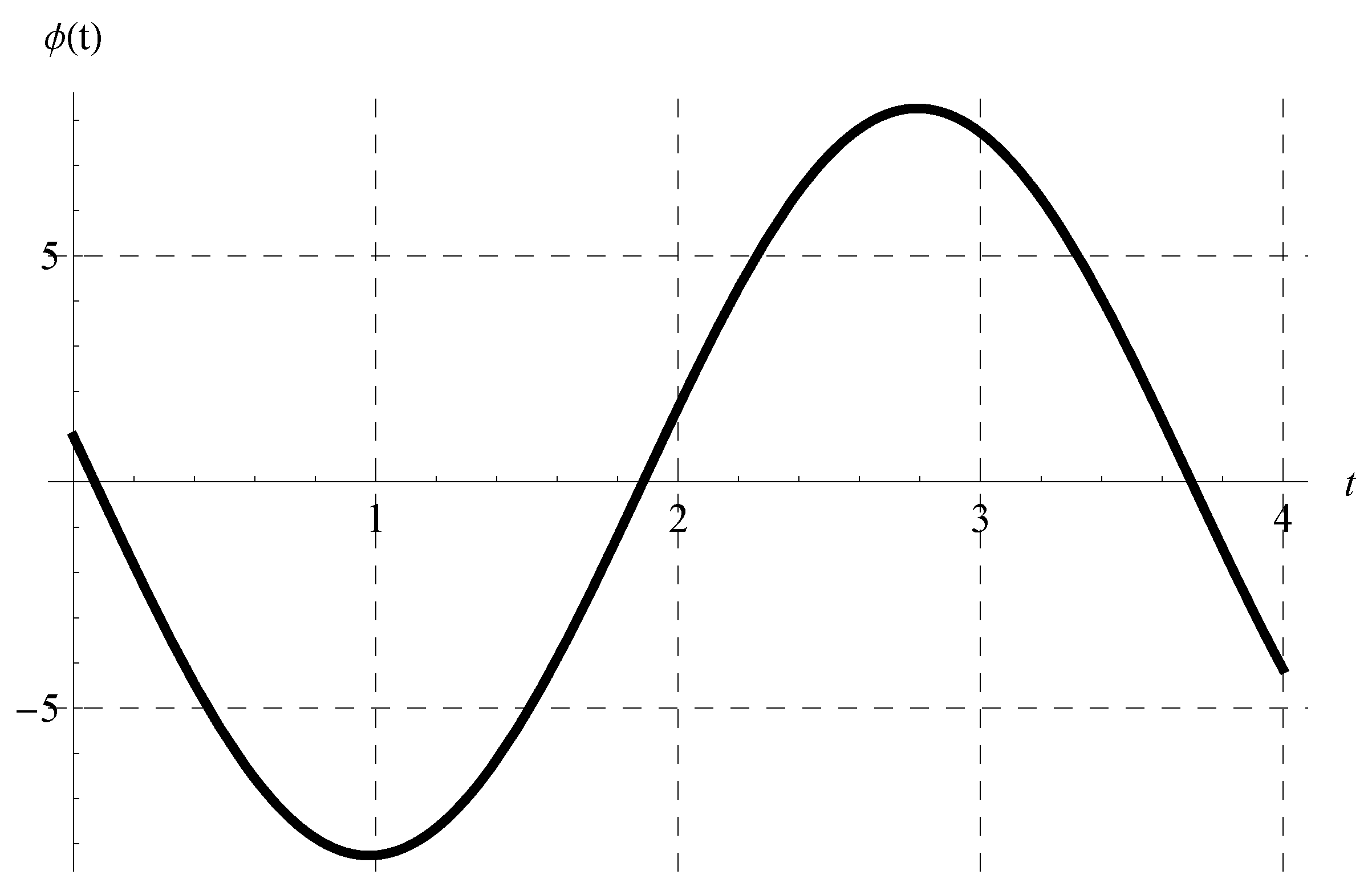
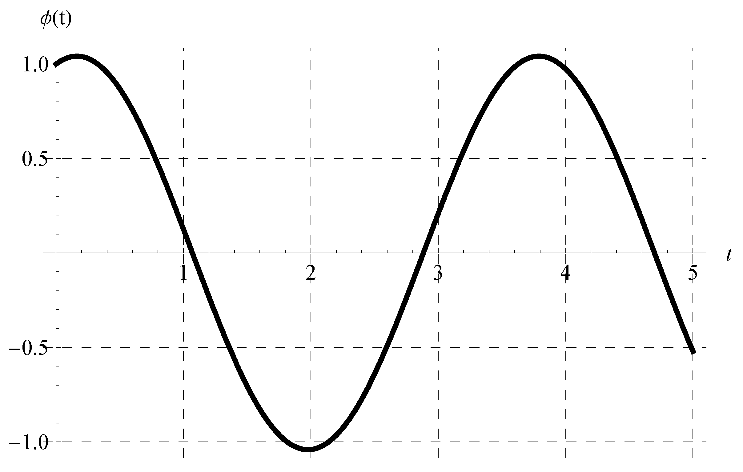
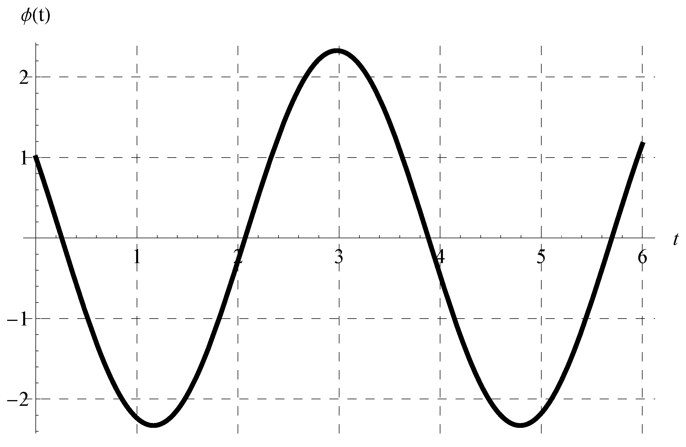
where $\Omega =\sqrt{{\beta }^2-{\alpha }^2}$ under the constraint $\left|\frac{\alpha }{\beta }\right|<1$. In view of Equation (46), the periodicity (P) is independent of the advance parameter ($\tau$). The chosen values of $\alpha$ and $\beta$ cover all possible cases regarding the signs of $\alpha$ and $\beta$ such that $\left|\frac{\alpha }{\beta }\right|<1$. Figure 1, Figure 2, Figure 3 and Figure 4 show the curves of the solution in the interval of $0\le t\le \tau /2$ (which is the domain of the solution of the present scalar model) at $\lambda =1$, $\alpha =1$, and $\beta =2$ when $\tau =6$ (Figure 1), $\tau =8$ (Figure 2), $\tau =10$ (Figure 3), and $\tau =12$ (Figure 4). Figure 1 and Figure 2 indicate that the curves represent portions of the periodic solution, i.e., not a complete period, while the curves depicted in Figure 3 and Figure 4 exceed a complete period in the domain of the solution. Moreover, the behavior of the solution at different values of $\alpha$ and $\beta$ is displayed in Figure 5 when $\lambda =1$ and $\tau =4$.

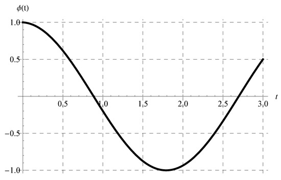
Figure 1. Plot of the solution at $\lambda =1$, $\alpha =1$, and $\beta =2$ when $\tau =6$.

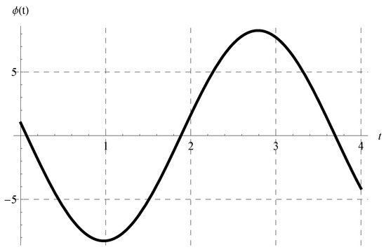
Figure 2. Plot of the solution at $\lambda =1$, $\alpha =1$, and $\beta =2$ when $\tau =8$.

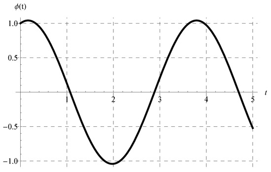
Figure 3. Plot of the solution at $\lambda =1$, $\alpha =1$, and $\beta =2$ when $\tau =10$.

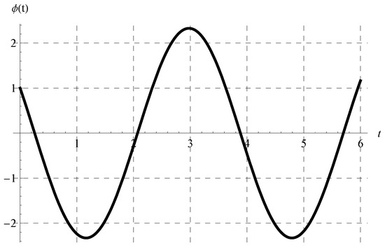
Figure 4. Plot of the solution at $\lambda =1$, $\alpha =1$, and $\beta =2$ when $\tau =12$.

Figure 5. Behavior of the solution at different values of $\alpha$ and $\beta$ when $\lambda =1$ and $\tau =4$.

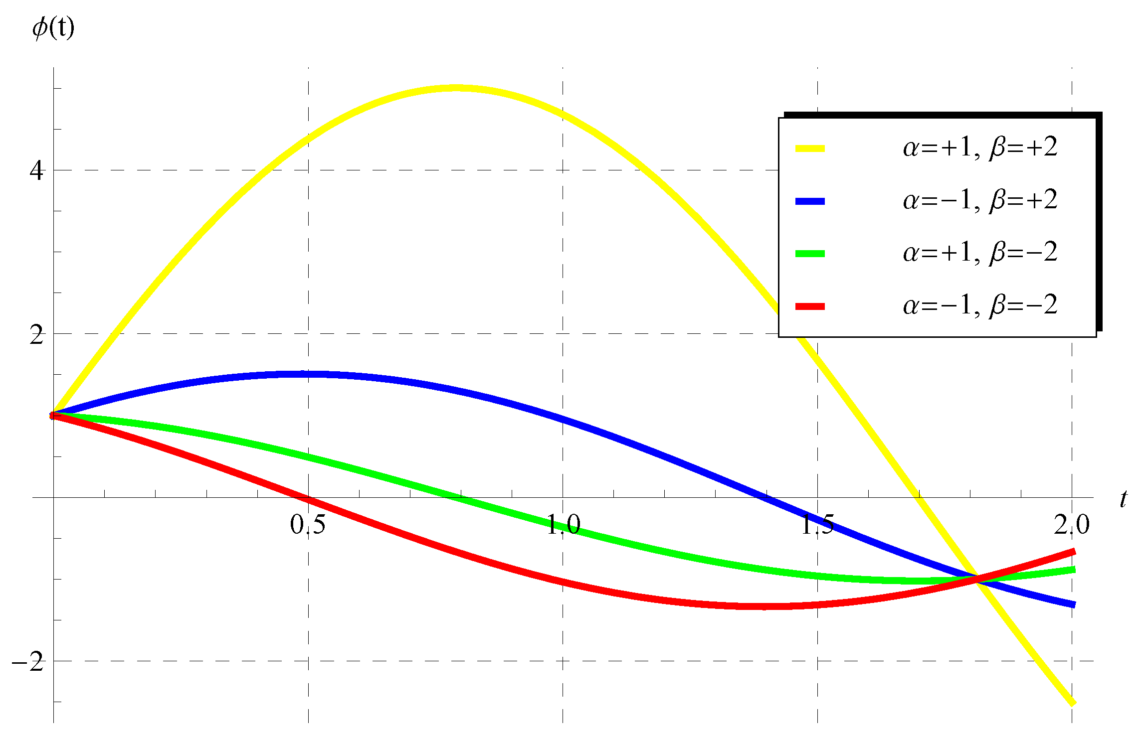
At a certain relation between the advance parameter ($\tau$) and the parameters $\alpha$ and $\beta$, one can obtain a solution with one complete period in the domain of $[0,\tau /2]$. Such a relation can be easily found, as $\tau /2=2\pi /\Omega$ which implies $\tau =4\pi /\sqrt{{\beta }^2-{\alpha }^2}$. In such a case, the exact periodic solution takes the following form:

$$\varphi \left(t\right)=\lambda \sqrt{\frac{2\beta }{\beta -\alpha }}sin\left(\sqrt{{\beta }^2-{\alpha }^2}t+{tan}^{-1}\left(\frac{\beta -\alpha }{\beta +\alpha }\right)\right),0\le t\le 2\pi /\sqrt{{\beta }^2-{\alpha }^2}.$$

(47)

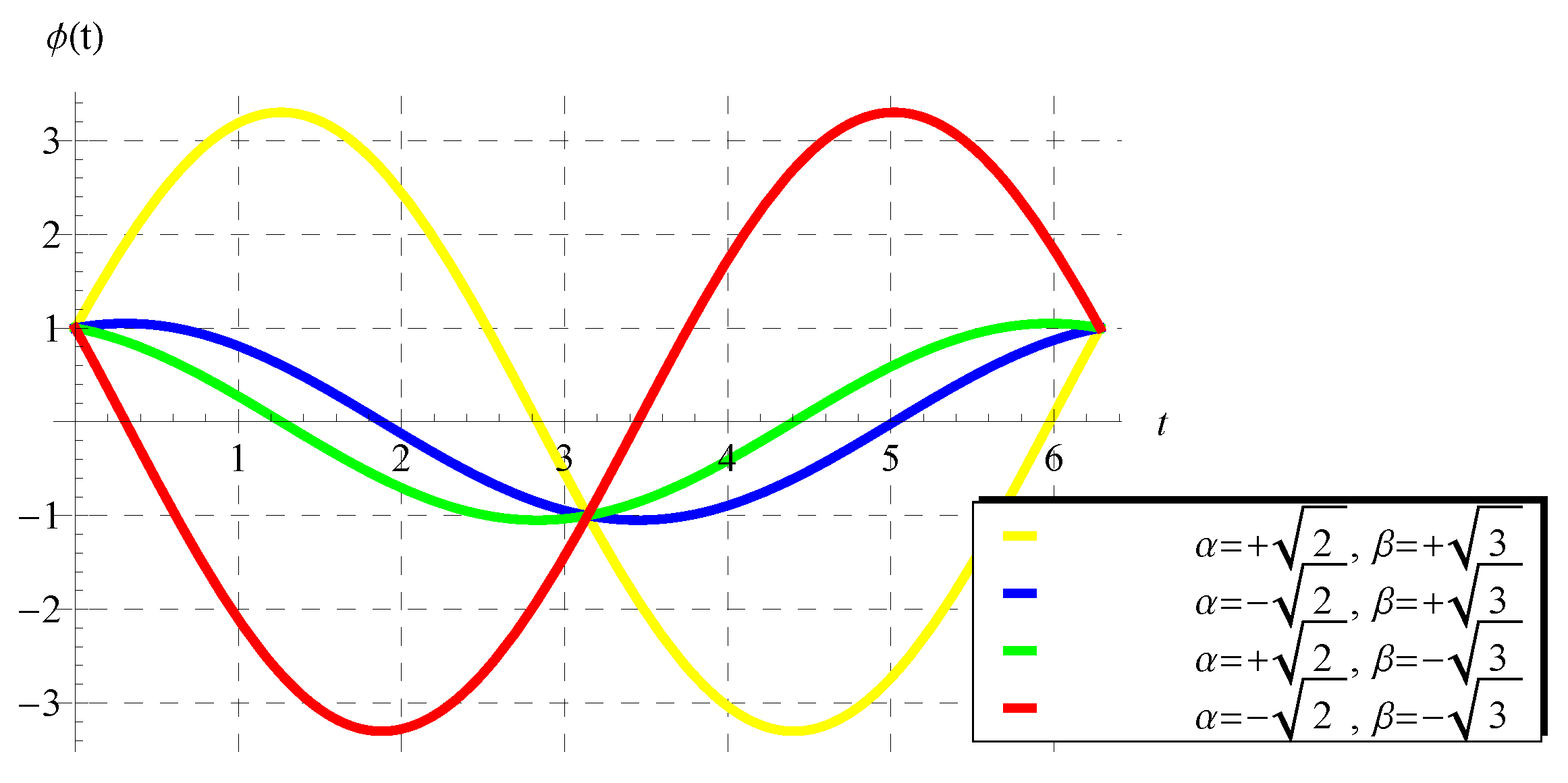
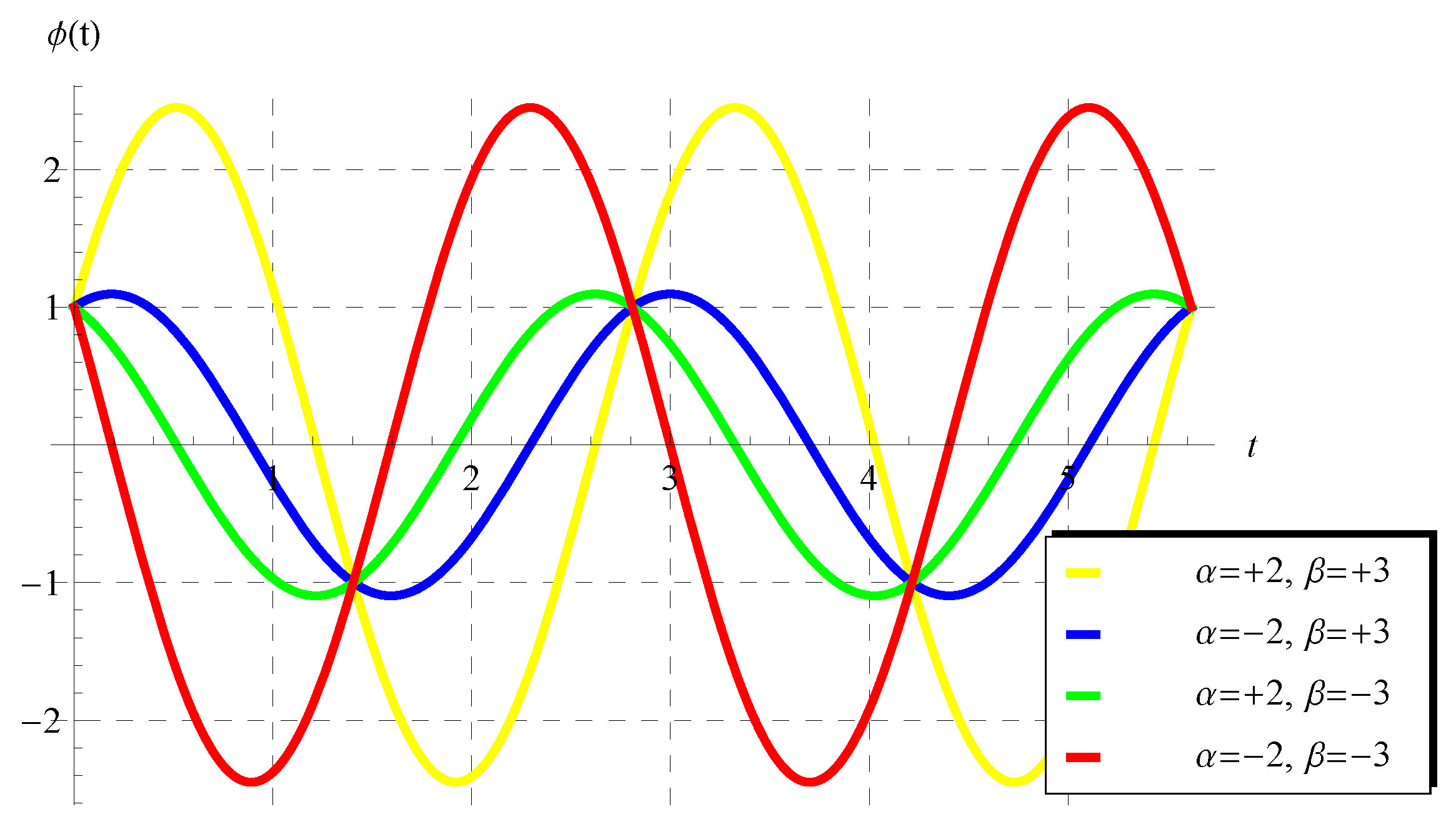
This form can be directly derived from Equation (26) (Theorem 1) by substituting $\Omega \tau /2=2\pi$. In addition, the solution in the form of (47) is invested to declare the curves in Figure 6. This figure shows four periodic solutions at four different selected values for the parameters $\alpha$ and $\beta$ ($(\alpha ,\beta )=(\pm 1,\pm 2)$) when $\lambda =1$ in the domain of one period ($0\le t\le 2\pi /\sqrt{3}$). Figure 7 shows four other periodic solutions at $(\alpha ,\beta )=(\pm \sqrt{2},\pm \sqrt{3})$ in the domain of $0\le t\le 2\pi$.

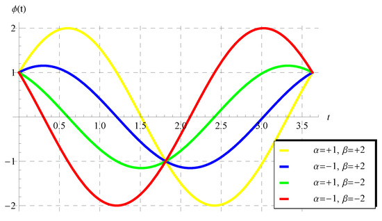
Figure 6. The periodic solution (47) for the scalar model (1) at $\lambda =1$ and some selected values of $\alpha$ and $\beta$ ($(\alpha ,\beta )=(\pm 1,\pm 2)$) in the domain of one period ($0\le t\le 2\pi /\sqrt{3}$).

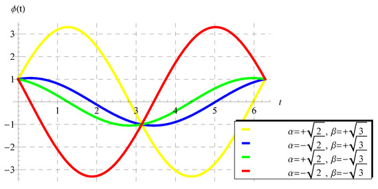
Figure 7. The periodic solution (47) for the scalar model (1) at $\lambda =1$ and some selected values of $\alpha$ and $\beta$ ($(\alpha ,\beta )=(\pm \sqrt{2},\pm \sqrt{3})$) in the domain of one period ($0\le t\le 2\pi$).

It is important to refer to the fact that Equation (47) is a solution for scalar (1) when $\tau =4\pi /\sqrt{{\beta }^2-{\alpha }^2}$, i.e.,

$${\varphi }^{\prime }\left(t\right)=\alpha \varphi \left(t\right)+\beta \varphi \left(-t+4\pi /\sqrt{{\beta }^2-{\alpha }^2}\right),\varphi \left(0\right)=\lambda ,$$

(48)

which consists of only one period in the range of $0\le t\le 2\pi /\sqrt{{\beta }^2-{\alpha }^2}$.

One can find a solution with two periods if the advance parameter ($\tau$) is chosen such that $\tau =8\pi /\sqrt{{\beta }^2-{\alpha }^2}$. In this case, the curves of the solution consist of two complete periods, as indicated in Figure 8.

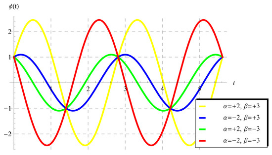
Figure 8. The periodic solution (47) for the scalar model (1) at $\lambda =1$ and some selected values of $\alpha$ and $\beta$ ($(\alpha ,\beta )=(\pm 2,\pm 5)$) in the domain of two periods ($0\le t\le 4\pi /\sqrt{5}$).

6.2. The Amplitude, Phase, and Critical Values of the Advance Parameter $\tau$: ${\tau }_c$

The amplitude ($\mathrm{Amplitude}\left(\varphi \right(t\left)\right)$) and the phase ($\mathrm{Phase}\left(\varphi \right(t\left)\right)$) of the wave/periodic solution ($\varphi \left(t\right)$) are mainly dependent on $\tau$, where

$$\begin{array}{cc}\hfill & \mathrm{Amplitude}\left(\varphi \right)=\lambda \sqrt{1+{\left(\frac{\Omega sin(\Omega \tau /2)+(\alpha +\beta )cos(\Omega \tau /2)}{\Omega cos(\Omega \tau /2)-(\alpha +\beta )sin(\Omega \tau /2)}\right)}^2},\hfill \\ \hfill & \mathrm{Phase}\left(\varphi \right)={tan}^{-1}\left(\frac{\Omega cos(\Omega \tau /2)-(\alpha +\beta )sin(\Omega \tau /2)}{\Omega sin(\Omega \tau /2)+(\alpha +\beta )cos(\Omega \tau /2)}\right).\hfill \end{array}$$

(49)

It is noticed from (49) that the amplitude of the wave is always greater than $\lambda$, i.e., $\mathrm{Amplitude}\left(\varphi \right)>\lambda$. However, we will show that $\mathrm{Amplitude}\left(\varphi \right)=\lambda$ at certain values of the advance parameter ($\tau$) (called the critical values, denoted as ${\tau }_c$). Setting $\Omega sin(\Omega \tau /2)+(\alpha +\beta )cos(\Omega \tau /2)=0$, we obtain

$$\tau ={\tau }_c=\frac{2}{\Omega }{tan}^{-1}\left(-\frac{\alpha +\beta }{\Omega }\right).$$

(50)

Inserting (50) into (49), one can obtain $\mathrm{Amplitude}\left(\varphi \right)=\lambda$.

6.3. Behavior of the Polynomial Solution

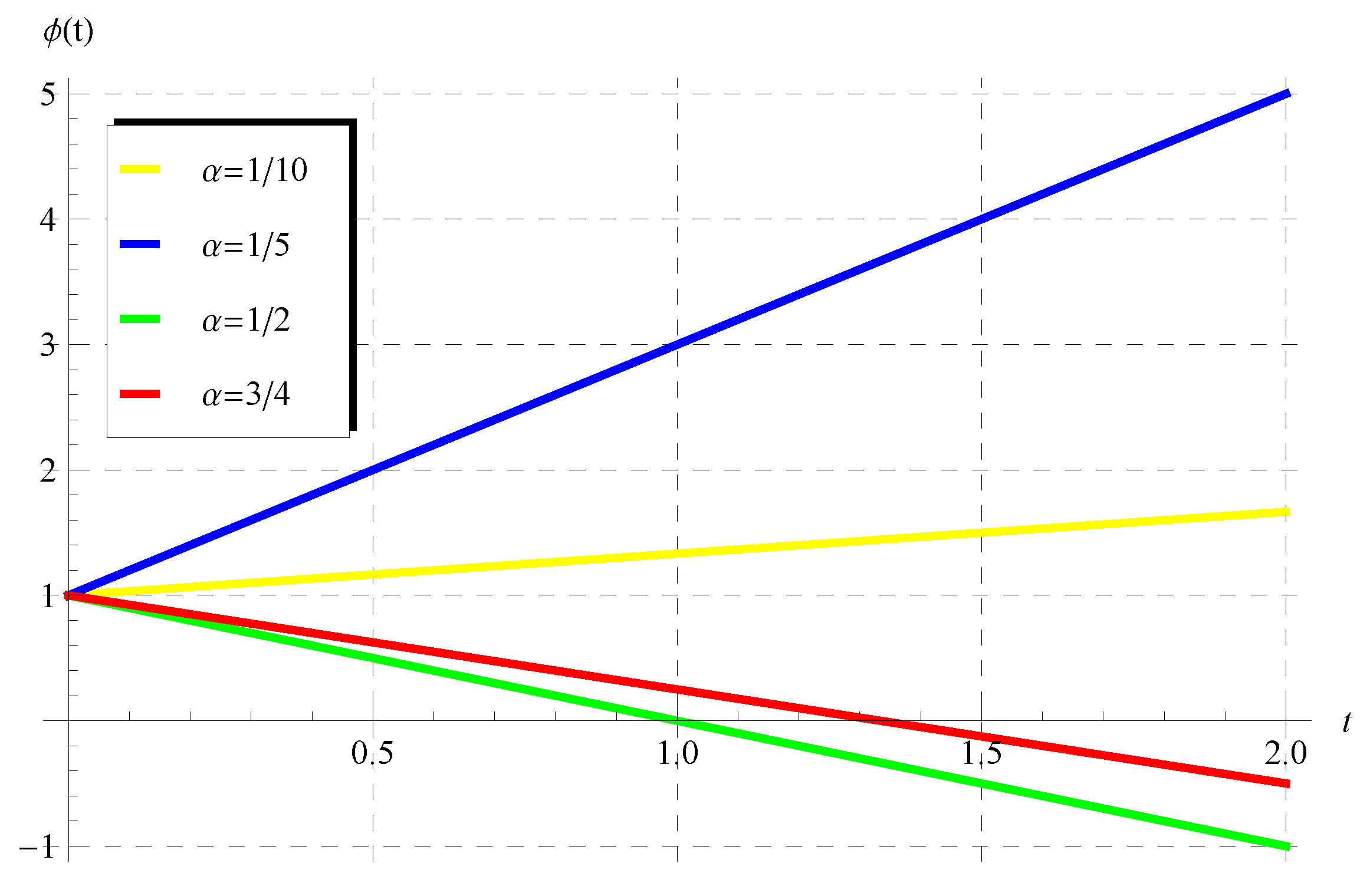
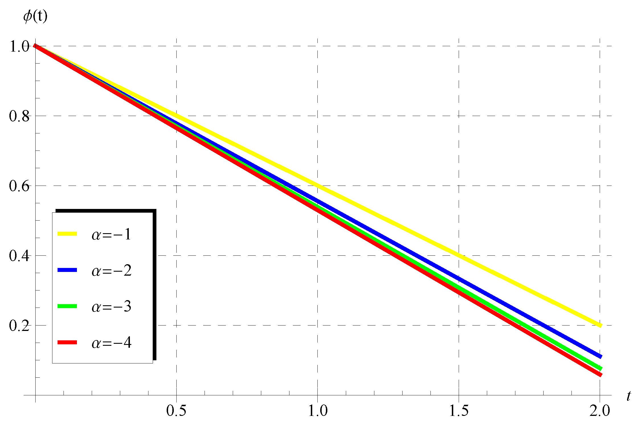
In Section 4, it was shown that model (1) has polynomial solution (39) when $\alpha =\beta$. In view of Equation (39), it can be deduced that $\varphi \left(t\right)$ is an increasing function in the whole domain of the independent variable (t) when $\alpha >0$ such that $\tau <1/\alpha$. However, $\varphi \left(t\right)$ decreases in the whole domain under two conditions/situations: the first occurs when $\alpha >0$ and $\tau >1/\alpha$, while the second condition requires $\alpha <0$ without any restrictions on the advance parameter ($\tau$). Such characteristics of the polynomial solution are demonstrated in Figure 9 and Figure 10.

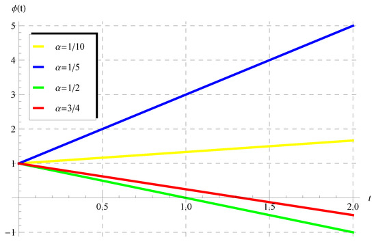
Figure 9. Behavior of the polynomial solution at different values of $\alpha >0$ when $\tau =4$ and $\lambda =1$.

Figure 10. Behavior of the polynomial solution at different values of $\alpha <0$ when $\tau =4$ and $\lambda =1$.

7. The Delay Equation: $\mathit{t}\ge \mathit{\tau }/\mathbf{2}$

The domain of the delay equation should be divided into two intervals ($\tau /2\le t\le \tau$ and $t>\tau$) because the properties of $\varphi \left(t\right)$ in one of these intervals are different than the properties in the other interval. The solution of the delay model is obtained by applying the method of steps in the intervals of $\tau /2\le t\le \tau$ and $t>\tau$; this is the issue of focus of the next subsections.

7.1. The Solution in the Interval: $\tau /2\le t\le \tau$

For $\tau /2\le t\le \tau$, we have $0\le -t+\tau \le \tau /2$; accordingly, the value of $\varphi (-t+\tau )$ can be evaluated from the solution in the interval of $[0,\tau /2]$. Let ${\varphi }_1\left(t\right)$ denote the solution in this interval; then, the delay model is described by

$${\varphi }^{\prime }\left(t\right)=\alpha \varphi \left(t\right)+\beta {\varphi }_1\left(-t+\tau \right),\varphi \left(t\right)={\varphi }_1\left(t\right)\forall t\in [0,\tau /2],\tau /2\le t\le \tau ,$$

(51)

with the following initial condition:

$$\varphi (\tau /2)={\varphi }_1(\tau /2)={\gamma }_1=\frac{\lambda \Omega }{\Omega cos(\Omega \tau /2)-(\alpha +\beta )sin(\Omega \tau /2)},$$

(52)

where ${\gamma }_1$ is obtained from Equation (25), and $\Omega$ is already defined in (18). Since ${\varphi }_1\left(t\right)$ is the solution for $t\in [0,\tau /2]$, according to (17), we can write

$${\varphi }_1(-t+\tau )=-c_{3}sin(\Omega (t-\tau ))+c_{4}cos(\Omega (t-\tau )),$$

(53)

where $c_3$ and $c_4$ were already obtained in Section 2.2. Inserting (53) into (51) and solving the IVP ((51) and (52)), we obtain the following exact solution:

$$\varphi \left(t\right)={\gamma }_1{e}^{\alpha \left(t-\frac{\tau }{2}\right)}+\frac{1}{\beta }\left[{\sigma }_{1}sin(\Omega t)-{\sigma }_{2}cos(\Omega t)-e^{\alpha \left(t-\frac{\tau }{2}\right)}\left({\sigma }_{1}sin(\Omega \tau /2)-{\sigma }_{2}cos(\Omega \tau /2)\right)\right],$$

(54)

where

$$\begin{gathered} {\sigma }_1=\Omega {\mu }_1-\alpha {\mu }_2,{\sigma }_2=\alpha {\mu }_1+\Omega {\mu }_2, \\ {\mu }_1=c_{4}cos(\Omega \tau )+c_{3}sin(\Omega \tau ),{\mu }_2=c_{4}sin(\Omega \tau )-c_{3}cos(\Omega \tau ). \end{gathered}$$

(55)

7.2. The Solution in the Interval of $t>\tau$

For $t>\tau$, we have $-t+\tau <0$; thus, the value of $\varphi (-t+\tau )$ vanishes in this case. Accordingly, the delay model reduces to the IVP, as follows:

$${\varphi }^{\prime }\left(t\right)=\alpha \varphi \left(t\right),\varphi \left(t\right)={\varphi }_2\left(t\right)\forall t\in [\tau /2,\tau ],t>\tau ,$$

(56)

where ${\varphi }_2\left(t\right)$ represents the solution ($\varphi \left(t\right)$) of Equation (54) in the interval of $[\tau /2,\tau ]$. Equation (56) is subjected to the following initial condition:

$$\varphi \left(\tau \right)={\varphi }_2\left(\tau \right)={\gamma }_2={\gamma }_1{e}^{\frac{\alpha \tau }{2}}+\frac{1}{\beta }\left[{\sigma }_{1}sin(\Omega \tau )-{\sigma }_{2}cos(\Omega \tau )-e^{\frac{\alpha \tau }{2}}\left({\sigma }_{1}sin(\Omega \tau /2)-{\sigma }_{2}cos(\Omega \tau /2)\right)\right],$$

(57)

where ${\gamma }_2$ is obtained from Equation (54). The solution of the present IVP reads

$$\varphi \left(t\right)={\gamma }_2{e}^{\alpha (t-\tau )},t>\tau .$$

(58)

8. Properties and Behavior of the Solution in the Full Domain

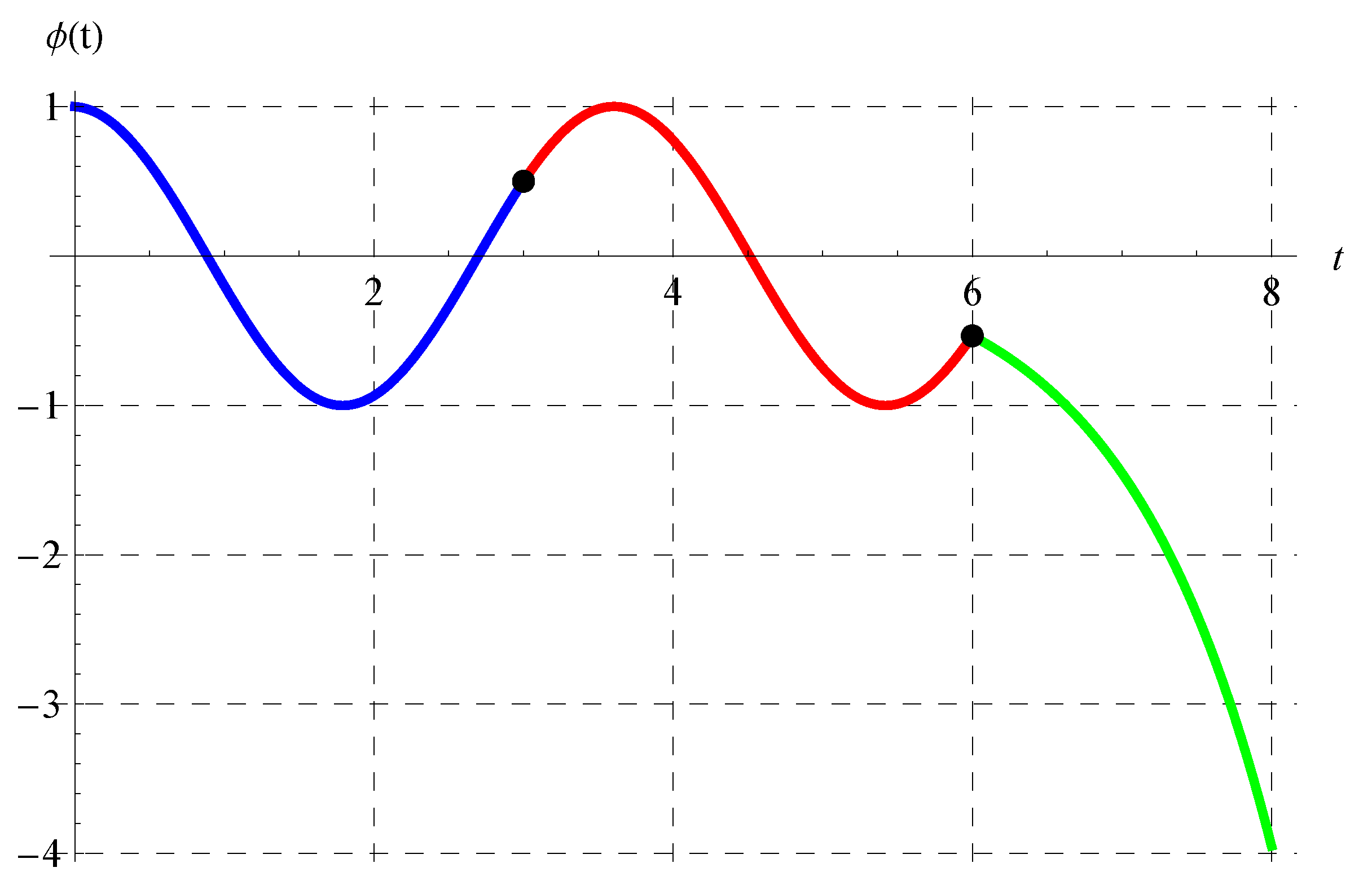
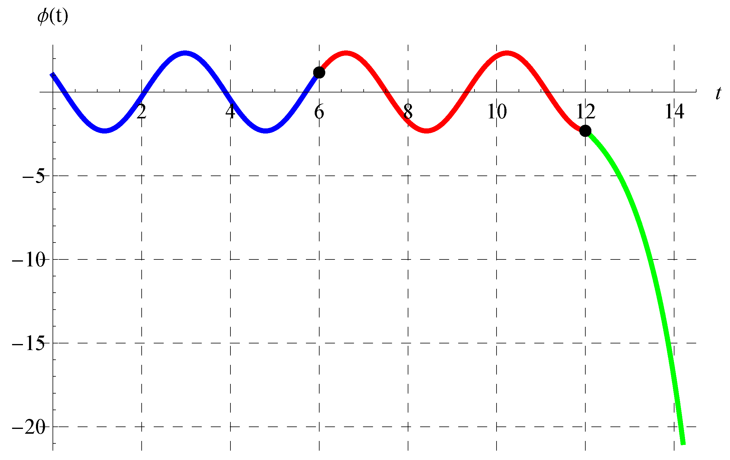
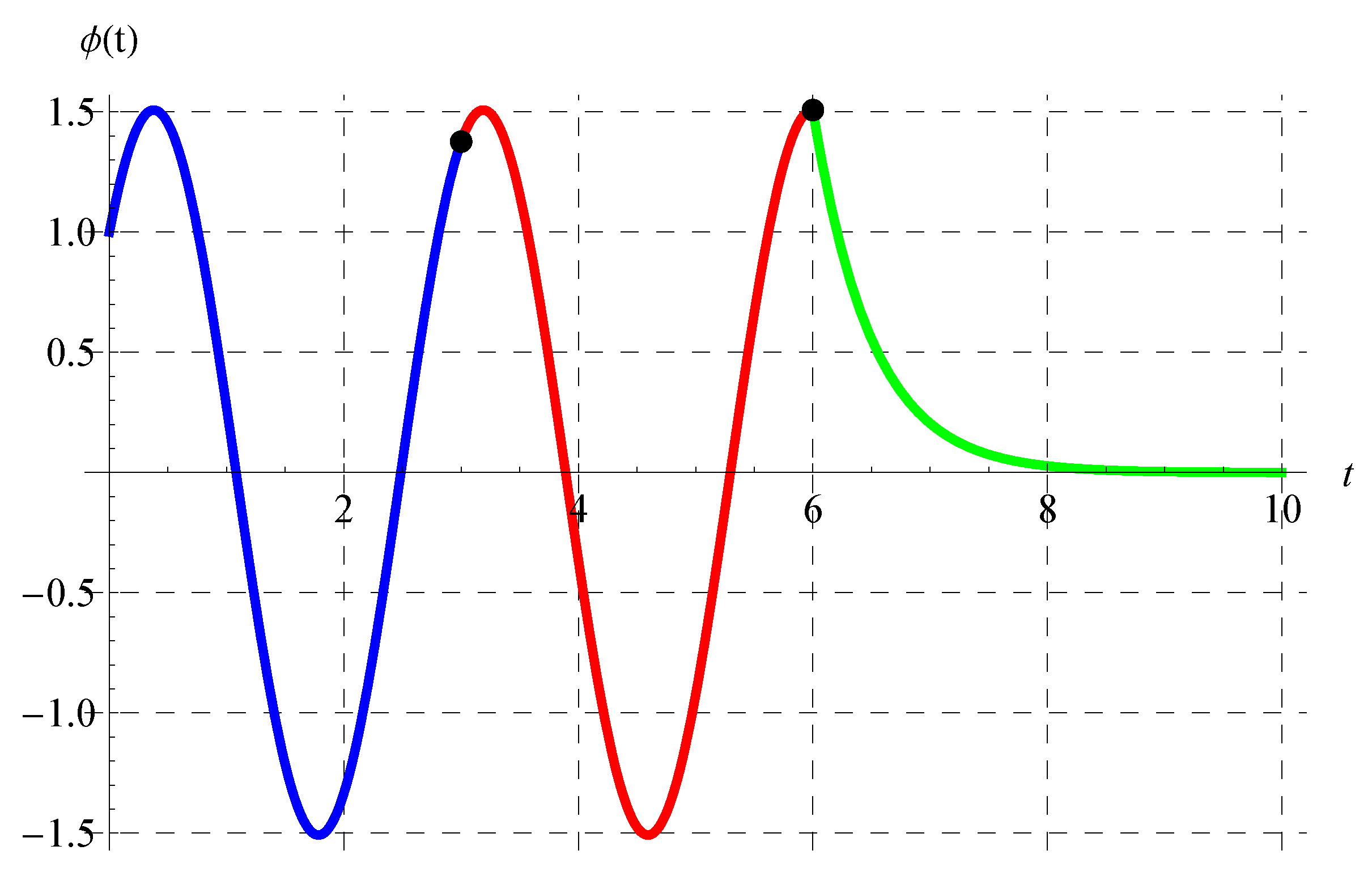
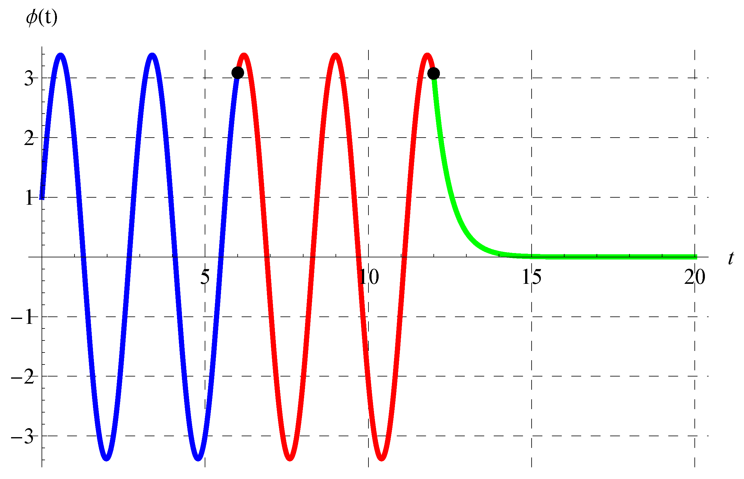
Figure 11, Figure 12, Figure 13 and Figure 14 show the curves of the solutions in the interval of $[0,\tau /2]$ for the advanced equation (blue curve) and in the intervals of $[\tau /2,\tau ]$ (red curve) and $(\tau ,\infty )$ (green curve) for the delay model. The black dots in these figures represent the connection points between the three solutions in the above three intervals. It is clear from Figure 11, Figure 12, Figure 13 and Figure 14 that $\varphi \left(t\right)$ is continuous. The oscillation of the solution is also obvious in the domain of $[0,\tau ]$, while another behavior occurs in the $(\tau ,\infty )$ domain.

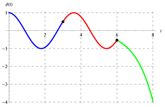
Figure 11. Plot of the solution in the interval of $[0,\tau /2]$ for the advanced equation (blue curve) and in the intervals of $[\tau /2,\tau ]$ (red curve) and $(\tau ,\infty )$ (green curve) for the delay equation. The black dots represent the connection points between the solutions at $\lambda =1$, $\alpha =1$, and $\beta =2$ when $\tau =6$.

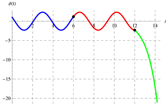
Figure 12. Plot of the solution in the interval of $[0,\tau /2]$ for the advanced equation (blue curve) and in the intervals of $[\tau /2,\tau ]$ (red curve) and $(\tau ,\infty )$ (green curve) for the delay equation. The black dots represent the connection points between the solutions at $\lambda =1$, $\alpha =1$, and $\beta =2$ when $\tau =12$.

Figure 13. Plot of the solution in the interval of $[0,\tau /2]$ for the advanced equation (blue curve) and in the intervals of $[\tau /2,\tau ]$ (red curve) and $(\tau ,\infty )$ (green curve) for the delay equation. The black dots represent the connection points between the solutions at $\lambda =1$, $\alpha =-2$, and $\beta =3$ when $\tau =6$.

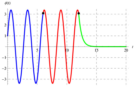
Figure 14. Plot of the solution in the interval of $[0,\tau /2]$ for the advanced equation (blue curve) and in the intervals of $[\tau /2,\tau ]$ (red curve) and $(\tau ,\infty )$ (green curve) for the delay equation. The black dots represent the connection points between the solutions at $\lambda =1$, $\alpha =-2$, and $\beta =3$ when $\tau =12$.

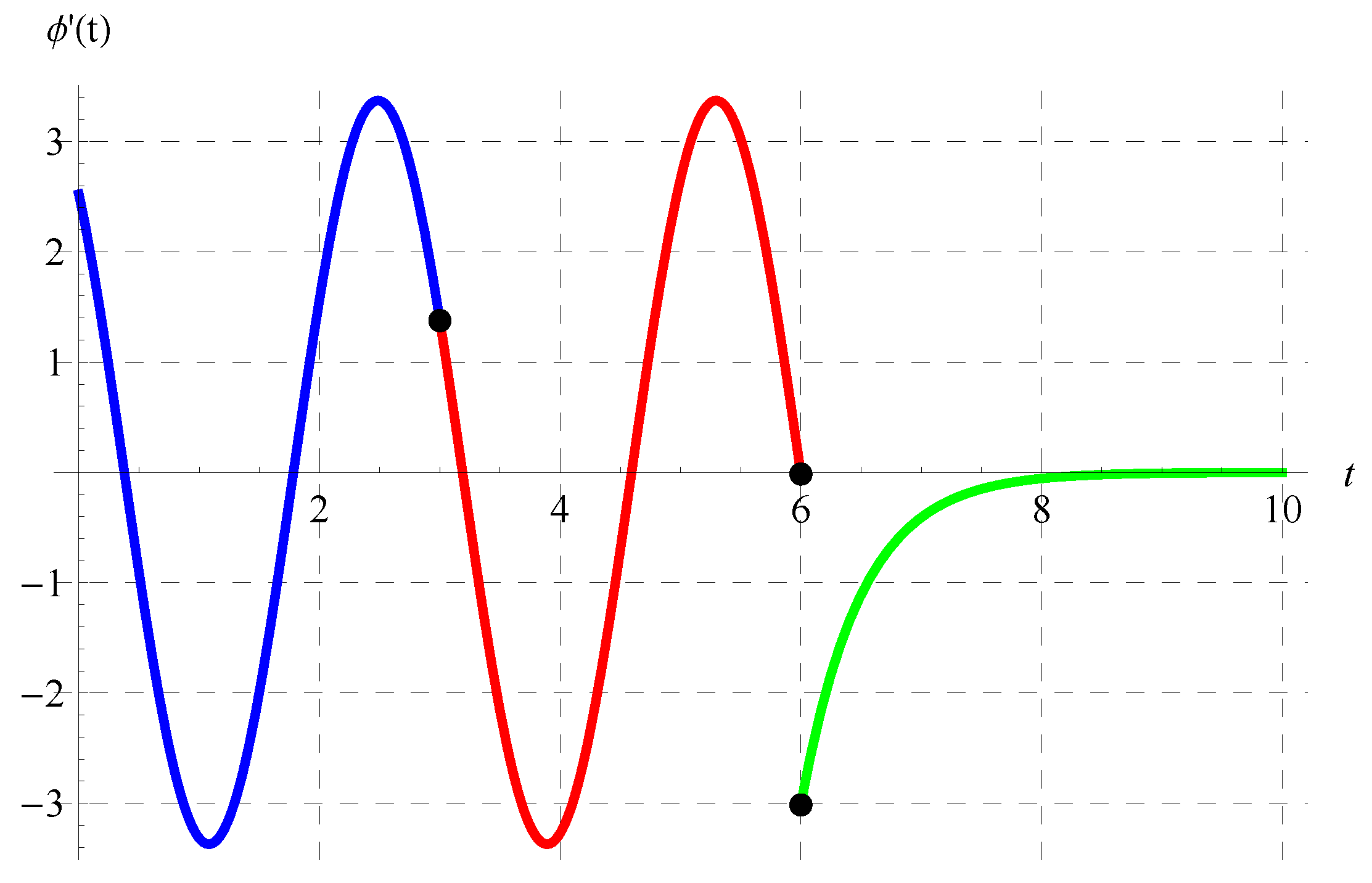
Figure 15, Figure 16, Figure 17 and Figure 18 display ${\varphi }^{\prime }\left(t\right)$ in the intervals of $[0,\tau /2]$ (blue curve), $[\tau /2,\tau ]$ (red curve), and $(\tau ,\infty )$ (green curve) at various values of the model’s parameters. It can be observed from these figures that ${\varphi }^{\prime }\left(t\right)$ is discontinuous at $t=\tau$, which is one of the main properties of the solution in the domain of the delay equation.

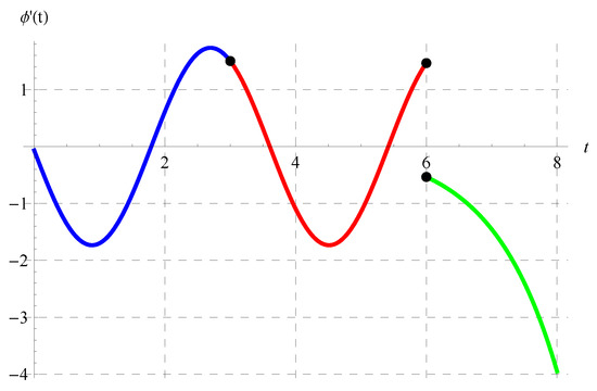
Figure 15. Plot of ${\varphi }^{\prime }\left(t\right)$ in the intervals of $[0,\tau /2]$ (blue curve), $[\tau /2,\tau ]$ (red curve), and $(\tau ,\infty )$ (green curve) at $\lambda =1$, $\alpha =1$, and $\beta =2$ when $\tau =6$.

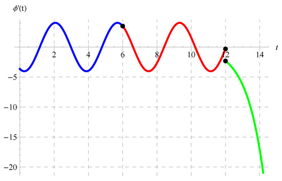
Figure 16. Plot of ${\varphi }^{\prime }\left(t\right)$ in the intervals of $[0,\tau /2]$ (blue curve), $[\tau /2,\tau ]$ (red curve), and $(\tau ,\infty )$ (green curve) at $\lambda =1$, $\alpha =1$, and $\beta =2$ when $\tau =12$.

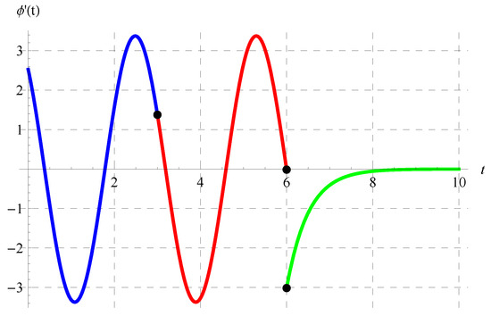
Figure 17. Plot of ${\varphi }^{\prime }\left(t\right)$ in the intervals of $[0,\tau /2]$ (blue curve), $[\tau /2,\tau ]$ (red curve), and $(\tau ,\infty )$ (green curve) at $\lambda =1$, $\alpha =-2$, and $\beta =3$ when $\tau =6$.

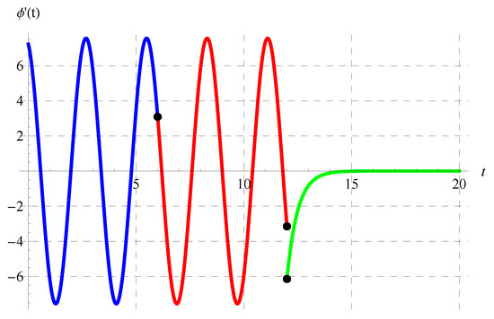
Figure 18. Plot of ${\varphi }^{\prime }\left(t\right)$ in the intervals of $[0,\tau /2]$ (blue curve), $[\tau /2,\tau ]$ (red curve), and $(\tau ,\infty )$ (green curve) at $\lambda =1$, $\alpha =-2$, and $\beta =3$ when $\tau =12$.

9. Conclusions

In this paper, a simple approach was presented to solve scalar equation ${\varphi }^{\prime }\left(t\right)=\alpha \varphi \left(t\right)+\beta \varphi \left(-t+\tau \right)$. An exact periodic solution was obtained under the condition of $\left|\frac{\alpha }{\beta }\right|<1$. A solution in the relevant literature at $\tau =0$ was recovered as a special case of the current case. In addition, a polynomial solution was deduced in terms of the advance parameter ($\tau$) when $\beta =\alpha$. It was demonstrated that the case of $\beta =-\alpha$ leads to a trivial/constant solution. The characteristics of the periodic and polynomial solutions were discussed in detail. Moreover, the behaviors of the periodic and polynomial solutions were introduced by means of several plots. The obtained results reveal the simplicity and the efficiency of the present analysis, which can be further extended to include other types of equations.

References

- Andrews, H.I. Third paper: Calculating the behaviour of an overhead catenary system for railway electrification. Proc. Inst. Mech. Eng. 1964, 179, 809–846. [Google Scholar] [CrossRef]
- Abbott, M.R. Numerical method for calculating the dynamic behaviour of a trolley wire overhead contact system for electric railways. Comput. J. 1970, 13, 363–368. [Google Scholar] [CrossRef]
- Gilbert, G.; Davtcs, H.E.H. Pantograph motion on a nearly uniform railway overhead line. Proc. Inst. Electr. Eng. 1966, 113, 485–492. [Google Scholar] [CrossRef]
- Caine, P.M.; Scott, P.R. Single-wire railway overhead system. Proc. Inst. Electr. Eng. 1969, 116, 1217–1221. [Google Scholar] [CrossRef]
- Ockendon, J.; Tayler, A.B. The dynamics of a current collection system for an electric locomotive. Proc. R. Soc. Lond. A Math. Phys. Eng. Sci. 1971, 322, 447–468. [Google Scholar]
- Fox, L.; Mayers, D.; Ockendon, J.R.; Tayler, A.B. On a functional differential equation. IMA J. Appl. Math. 1971, 8, 271–307. [Google Scholar] [CrossRef]
- Kato, T.; McLeod, J.B. The functional-differential equation y′(x)=ay(λx)+by(x). Bull. Am. Math. Soc. 1971, 77, 891–935. [Google Scholar]
- Iserles, A. On the generalized pantograph functional-differential equation. Eur. J. Appl. Math. 1993, 4, 1–38. [Google Scholar] [CrossRef]
- Ambartsumian, V.A. On the fluctuation of the brightness of the milky way. Dokl. Akad. Nauk USSR 1994, 44, 223–226. [Google Scholar]
- Patade, J.; Bhalekar, S. On analytical solution of Ambartsumian equation. Natl. Acad. Sci. Lett. 2017, 40, 291–293. [Google Scholar] [CrossRef]
- Bakodah, H.O.; Ebaid, A. Exact solution of Ambartsumian delay differential equation and comparison with Daftardar-Gejji and Jafari approximate method. Mathematics 2018, 6, 331. [Google Scholar] [CrossRef]
- Khaled, S.M.; El-Zahar, E.R.; Ebaid, A. Solution of Ambartsumian delay differential equation with conformable derivative. Mathematics 2019, 7, 425. [Google Scholar] [CrossRef]
- Kumar, D.; Singh, J.; Baleanu, D.; Rathore, S. Analysis of a fractional model of the Ambartsumian equation. Eur. Phys. J. Plus 2018, 133, 133–259. [Google Scholar] [CrossRef]
- Ebaid, A.; Al-Jeaid, H.K. On the exact solution of the functional differential equation y′(t)=ay(t)+by(-t). Adv. Differ. Equ. Control Process. 2022, 26, 39–49. [Google Scholar]
- Adomian, G. Solving Frontier Problems of Physics: The Decomposition Method; Kluwer Acad: Boston, MA, USA, 1994. [Google Scholar]
- Wazwaz, A.M. Adomian decomposition method for a reliable treatment of the Bratu-type equations. Appl. Math. Comput. 2005, 166, 652–663. [Google Scholar] [CrossRef]
- Duan, J.S.; Rach, R. A new modification of the Adomian decomposition method for solving boundary value problems for higher order nonlinear differential equations. Appl. Math. Comput. 2011, 218, 4090–4118. [Google Scholar] [CrossRef]
- Diblík, J.; Kúdelcíková, M. Two classes of positive solutions of first order functional differential equations of delayed type. Nonlinear Anal. Theory Methods Appl. 2012, 75, 4807–4820. [Google Scholar] [CrossRef]
- Alshaery, A.; Ebaid, A. Accurate analytical periodic solution of the elliptical Kepler equation using the Adomian decomposition method. Acta Astronaut. 2017, 140, 27–33. [Google Scholar] [CrossRef]
- Li, W.; Pang, Y. Application of Adomian decomposition method to nonlinear systems. Adv. Differ. Equ. 2020, 2020, 67. [Google Scholar] [CrossRef]
- Ebaid, A.; Al-Jeaid, H.K.; Al-Aly, H. Notes on the Perturbation Solutions of the Boundary Layer Flow of Nanofluids Past a Stretching Sheet. Appl. Math. Sci. 2013, 7, 6077–6085. [Google Scholar] [CrossRef]
- Ebaid, A. Remarks on the homotopy perturbation method for the peristaltic flow of Jeffrey fluid with nano-particles in an asymmetric channel. Comput. Math. Appl. 2014, 68, 77–85. [Google Scholar] [CrossRef]
- Ayati, Z.; Biazar, J. On the convergence of Homotopy perturbation method. J. Egypt. Math. Soc. 2015, 23, 424–428. [Google Scholar] [CrossRef]
- Khaled, S.M. The exact effects of radiation and joule heating on Magnetohydrodynamic Marangoni convection over a flat surface. Therm. Sci. 2018, 22, 63–72. [Google Scholar] [CrossRef]
Disclaimer/Publisher’s Note: The statements, opinions and data contained in all publications are solely those of the individual author(s) and contributor(s) and not of MDPI and/or the editor(s). MDPI and/or the editor(s) disclaim responsibility for any injury to people or property resulting from any ideas, methods, instructions or products referred to in the content. |
© 2024 by the authors. Licensee MDPI, Basel, Switzerland. This article is an open access article distributed under the terms and conditions of the Creative Commons Attribution (CC BY) license (https://creativecommons.org/licenses/by/4.0/).